spss/excel workshop 2 –semester one, 2010leila/10s1_spss_excel_workshop_ii.… · spss/excel...

STUDENT LEARNING CENTRE 3rd Floor

Information Commons

© Student Learning Centre The University of Auckland 1

SPSS/Excel Workshop 2 –Semester One, 2010 In Assignment 2 of STATS 10x you may want to use Excel or SPSS to perform some calculations, that is, finding Normal probabilities and Inverse Normal values in Question 3.

You may also like to use Excel and SPSS to check you’ve done your ‘by hand’ calculations correctly for your confidence intervals in Questions 5 and 6.

Instructions from your assignment sheet read:

Question guide

• Question 3 will require use of Excel, SPSS or a graphics calculator for calculating probabilities

from Normal distributions. Do not hand in any computer output for these questions. Use Excel,

SPSS or a graphics calculator to find the solutions. DO NOT USE TABLES.

Question 3. [9 marks] [Chapter 6]

Reminder: When calculating Normal probabilities, use SPSS, Excel or a graphics calculator.

Do not use tables. Report any probabilities to 4 decimal places.

On the following pages are some questions from the Worked Examples document which you can find on Cecil.

Question 6 [Chapter 6] (helpful for Question 3, Assignment 2)

A medical trial was conducted to investigate whether a new drug extended the

life of a patient who had lung cancer. The survival times (in months) for 38

cancer patients who were treated with the drug are as follows:

1, 1, 5, 9, 10, 13, 14, 17, 18, 18, 19, 21, 22, 25, 25, 25, 26, 27, 29,

36, 38, 39, 39, 40, 41, 41, 43, 44, 44, 45, 46, 46, 49, 50, 50, 54, 54, 59.

Sample mean ≈ 31.1 months and sample standard deviation ≈ 16.0 months.

Assume that the survival time (in months) for patients on this drug is Normally

distributed with a mean of 31.1 months and a standard deviation of 16.0

months.

(i) What is the probability that a patient survives for no more than one

year?

(ii) What percentage of patients survive for at least two years?

(iii) What proportion of patients will survive between one year and two

years?

(iv) What is the highest survival time that 80% of patient survival times

exceed?

(v) What is the lower quartile of the survival times?

(vi) Calculate the central 80% of survival times.


Information Commons


Question 6 Solutions

Let X be the survival time ( ) for a patient on the drug.

X ~ Normal (µ = __________, σ = __________)

(i) Pr( X )

= (4dp)

(ii) Pr( X )

=

=

= (2dp)

(iii) Pr( )

= Pr( ) – Pr( )

=

= (4dp)

(iv) We want to calculate x such that Pr( X ≥ x ) =

⇒ Pr( X ≤ x ) =

⇒ x = (1dp)

The highest survival time that 80% of patient survival times exceed is

__________ months.

µ=

µ=

µ=

µ=


Information Commons


(v) We want to calculate x such that Pr(X ≤ x) =

⇒ x = (1dp)

The lower quartile of the survival times is __________ months.

(vi) For the central 80% of survival times: Pr(xL ≤ X ≤ xU) = 0.80

⇒ Pr(X ≤ xL) =

⇒ xL = (1dp)

Pr(xL ≤ X ≤ xU) = 0.80

⇒ Pr(X ≤ xU) =

⇒ xU = (1dp)

The central 80% of survival times fall between __________ months and

__________ months.

Excel

Calculating Normal Probabilities A. Lower tail probabilities: Pr(X ≤≤≤≤ x)

Example: Find Pr(X ≤ 5) where X ~ Normal(µ = 7, σ = 6)

1. Click in cell A1.

2. Click the Insert Function button from beside the formula bar.

3. Choose Statistical from the Or select a category box in the Insert

Function dialog box.

µ=

µ=


Information Commons


4. Choose NORMDIST from the Select a function box (Figure 1).

Figure 1

5. Click OK.

6. Fill in the NORMDIST dialog box (Figure 2).

Figure 2

where:

X is the value for which we want the distribution. It is

equivalent to x in our manual. In this example, we put

5 in this box.

Mean is the mean of the distribution. It is equivalent to µ in

our manual. In this example, we put 7 in this box.


Information Commons


Standard_dev is the standard deviation of the distribution. It is

equivalent to σ in our manual. In this example, we put 6

in this box.

Cumulative indicates whether we want a cumulative distribution

function (TRUE or 1) or a probability mass function

(FALSE or 0). We will always put TRUE or 1 in this box.

7. Click OK. (The value of 0.369 should appear in cell A1.)

B. Upper tail probabilities: Pr(X ≥≥≥≥ x)

Example: Find Pr(X ≥ 9) where X ~ Normal(µ = 7, σ = 6)

Note: Pr(X ≥ 9) = 1 – Pr(X ≤ 9)

1. Evaluate Pr(X ≤ 9) in cell B1 (use steps in A).

2. In cell B2, type: =1 – B1.

3. Press Enter. (The value of 0.369 should appear in cell B2.)

C. Pr(a ≤≤≤≤ X ≤≤≤≤ b)

Example: Find Pr(5 ≤ X ≤ 11) where X ~ Normal(µ = 7, σ = 6)

Note: Pr(5 ≤ X ≤ 11) = Pr(X ≤ 11) – Pr(X ≤ 5)

1. Evaluate Pr(X ≤ 11) in cell C1 (use steps in A).

2. Evaluate Pr(X ≤ 5) in cell C2 (use steps in A).

3. In cell C3, type: =C1 – C2.

4. Press Enter. (The value of 0.378 should appear in cell C3.)


Information Commons


Note:

Another way to calculate Normal probabilities is to type the function

=NORMDIST(x, µ, σ, c) directly into a cell, where:

x is the value for which we want the distribution.

µ is the mean of the distribution.

σ is the standard deviation of the distribution

c is always 1.

For example:

To evaluate Pr(X ≤ 5): In cell A1, type: =NORMDIST(5, 7, 6, 1).

To evaluate Pr(X ≥ 9): In cell B1, type: =NORMDIST(9, 7, 6, 1)

In cell B2, type: =1 – B1.

To evaluate Pr(5 ≤ X ≤ 11): In cell C1, type: =NORMDIST(11, 7, 6, 1).

In cell C2, type: =NORMDIST(5, 7, 6, 1).

In cell C3, type: =C1 – C2.

Figure 3


Information Commons


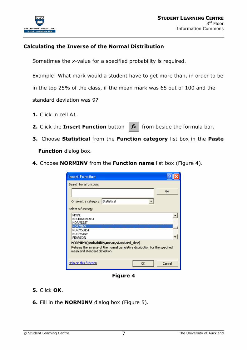
Calculating the Inverse of the Normal Distribution

Sometimes the x-value for a specified probability is required.

Example: What mark would a student have to get more than, in order to be

in the top 25% of the class, if the mean mark was 65 out of 100 and the

standard deviation was 9?



3. Choose Statistical from the Function category list box in the Paste


4. Choose NORMINV from the Function name list box (Figure 4).

Figure 4

5. Click OK.

6. Fill in the NORMINV dialog box (Figure 5).


Information Commons


Figure 5

Note: the Excel function NORMINV determines the x-value for the

probability that is to the left of the required x-value. In this

example we want the top 25% therefore we use 1 – 0.25, or 0.75

for the probability. If instead we wanted the bottom 25% the

probability is 0.25.

7. Click OK. (The value of 71.0704 should appear in cell A1.)

Note:

The formula can be directly entered into the cell by typing =NORMINV(p, µ, σ), where:

p is the probability to the left of the x-value being calculated

µ is the mean of the distribution

σ is the standard deviation of the distribution

Note:

Excel has two other functions that work in the same manner as the

functions explained above. These two functions are NORMSDIST and

NORMSINV. These two functions calculate the value for a standard normal

distribution,

ie. X ~ Normal(0, 1).


Information Commons


Calculating the t-multiplier

(Calculating the Inverse of the Student t-distribution)

Example: Find the t-multiplier for a 95% confidence interval with degrees

of freedom, df = 29. (That is: t29(0.025), probability 0.025 and 29 degrees

of freedom).



3. Choose Statistical from the Or select a category box in the Insert


4. Choose TINV from the Select a function box (Figure 4).

Figure 4


Information Commons


5. Click OK

6. Fill in the TINV dialog box (Figure 5).

Figure 5

Note:

The Excel function TINV calculates the t-value for two–tailed t-distribution. So

if we want to find the t-value whose probability to the right is 0.1, then in the

TINV function the value for the probability is entered as 0.2, because of the

two-tailed nature of the function.

7. Click OK. (The value 2.045 should appear in cell A1.)

Note:

The example can be solved by directly typing the formula =TINV(p, df) into

the cell, where:

p is the probability for the two-tailed distribution

df is the number of degrees of freedom for the distribution


Information Commons


Useful places to look for help by assignment question

Assignment question number

Worked

Examples question number

Lecture

Workbook page

number

Q1

Q2

Q3

Q4

Q5

Q6

Also, don’t forget where else you can get assignment help! They are:

• Your lecturer’s office hours! See Cecil for details – if they don’t suit you, email or call them to book a time.

• Statistics Assistance Area – ask a tutor or your neighbour

• Statistics Computer Lab – ask a lab demonstrator or your neighbour

• The STATS 10x forum: www.stat.auckland.ac.nz/forum/10x


Information Commons


Downloading the Excel Test and Confidence Interval Calculators

These are available to you in two places:

1. From Cecil (log in to Cecil in the usual way, click on Assignment Resources and look for “Single proportion/One proportion” and “Two proportions”

2. Go to Leila’s Student Learning Centre STATS 10x webpage www.stat.auckland.ac.nz/~leila

Whichever way you do it, access Two proportions.xls now.

Let’s have a go at using the Two proportions.xls document!

We won’t be doing the calculations by hand, although you are welcome to try later – in this workshop we’ll use Excel to do them!


Information Commons


Question 10 [Chapter 8] (similar to Question 6, Assignment 2)

In April 1996 the New Zealand Consumers' Institute conducted a survey on

home computer use. 7400 subscribers to Consumer Magazine were randomly

selected and sent a survey form. Of those surveyed, 2730 had a computer for

personal use at home. The respondents who had a home computer were given

a list of computer activities and were asked to indicate all of those that they

engaged in. They were also asked to indicate the number of hours per week

that they used their computer. The Consumers' Institute used the results to

draw conclusions about subscribers who own a home computer. The results

of the survey are given in the two tables below.

Computer Activities Computer Use

(hours per week)

Word-processing 2621 Not used 27

Games 1502 Used for less than 2 hours 328

Spreadsheets 819 Over 2 and up to 7 hours (incl) 764

Accounting 655 Over 7 and up to 14 hours (incl) 710

Databases 437 Over 14 and up to 21 hours (incl) 546

Internet 328 Over 21 and up to 28 hours (incl) 109

Drawing 300 Over 28 and up to 35 hours (incl) 136

Desktop publishing 246 Over 35 and up to 44 hours (incl) 55

Fax / answering machine 82 Over 44 hours 55

Total 2730

(c) Identify the sampling situation as (a) Two independent samples, (b)

Single sample, several response categories or (c) Single sample, two or

more Yes/No items in the following cases:

(i) Consider the results from the New Zealand Consumers' Institute

survey on home computer use above. We want to compare the

proportion of respondents who use their home computer for

spreadsheets with the proportion of respondents who use their home

computer for accounting.

(ii) Consider the results from the New Zealand Consumers' Institute

survey on home computer use above. We want to compare the

proportion of respondents who use their home computer for over 7

and up to 14 hours per week and the proportion of respondents who

use their home computer for over 14 and up to 21 hours per week.


Information Commons


(iii) As part of a nationwide telephone survey in 1998, data was collected

on people who use their home computers for Internet activities. We

want to compare the proportion of respondents (in this survey) who

use their home computer for the Internet to the proportion of

respondents from the Consumers' Institute survey who use their home

computer for the Internet.

(d) By hand, calculate a 95% confidence interval for the difference between

the proportion of people who use their computer for drawing and the

proportion of people who use their computer for desktop publishing.

Interpret your results.

1 Parameter = pD – p

P, the difference in the true proportion of people

with a home computer who use it for drawing and the true

proportion who use it for desktop publishing.

2 Estimate PD pp ˆˆ −= , the difference in the proportion of respondents

with a home computer who use it for drawing and the proportion

who use it for desktop publishing.

= 0198.00901.01099.02730

246

2730

300ˆˆ =−=−=− PD pp

3 Formula = estimate ± t × se(estimate) gives

)ˆˆ(se)ˆˆ( PDPD pptpp −×±−

4 Situation (c): One sample, two or more Yes/No items.

2.00901.01099.0ˆˆ =+=+ PD pp , 8.19099.08901.0ˆˆ =+=+ PD qq

008551.0008550816.02730

0198.02.0)ˆˆ(se

2

≈=−

=− PD pp

5 df = ∞ (working with proportions)

6 For a 95% confidence interval with df = ∞, use t = z = 1.96

7 95% confidence interval is: )ˆˆ(se)ˆˆ( PDPD ppzpp −×±−

= 0.0198 ± 1.96 × 0.008551

= 0.0198 ± 0.016760

= (0.0030, 0.0366)

8 With 95% confidence, we estimate that the true proportion of people

with a home computer who use it for drawing to be up to 0.04

higher than the true proportion who use it for desktop publishing.


Information Commons


SPSS

One Sample Example: There is interest in quantifying the nitrate ion concentration in a

water supply. The concentration in a specimen of the water was measured 10 times.

1. Enter the data into SPSS or download NitrateIon.sav from Cecil or

www.stat.auckland.ac.nz/~leila. Label Conc as Concentration.

2. Choose the analysis tool: One-Sample T Test. Click Analyze → Compare Means → One-Sample T Test.


Information Commons


3. Select the relevant variable(s). Click Concentration [Conc].

Click .

4. Click OK.

5. View and interpret the results.

spss/excel workshop 2 –semester one, 2010leila/10s1_spss_excel_workshop_ii.… · spss/excel...

Documents