splines jehee lee seoul national university. particle motion a curve in 3-dimensional space world...
TRANSCRIPT

Splines
Jehee Lee
Seoul National University

Particle Motion
• A curve in 3-dimensional space
World coordinates
)(),(),()( tztytxt p

Keyframing Particle Motion
• Find a smooth function that passes through given keyframes
World coordinates
),( 00 pt
),( 11 pt
),( 22 pt
),( 33 pt
.0),,( nit ii p)(tp
Polynomial Curve
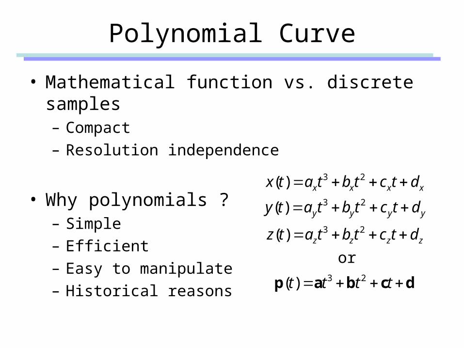
• Mathematical function vs. discrete samples– Compact– Resolution independence
• Why polynomials ?– Simple– Efficient– Easy to manipulate– Historical reasons
dcbap
tttt
dtctbtatz
dtctbtaty
dtctbtatx
zzzz
yyyy
xxxx
23
23
23
23
)(
or
)(
)(
)(
Degree and Order
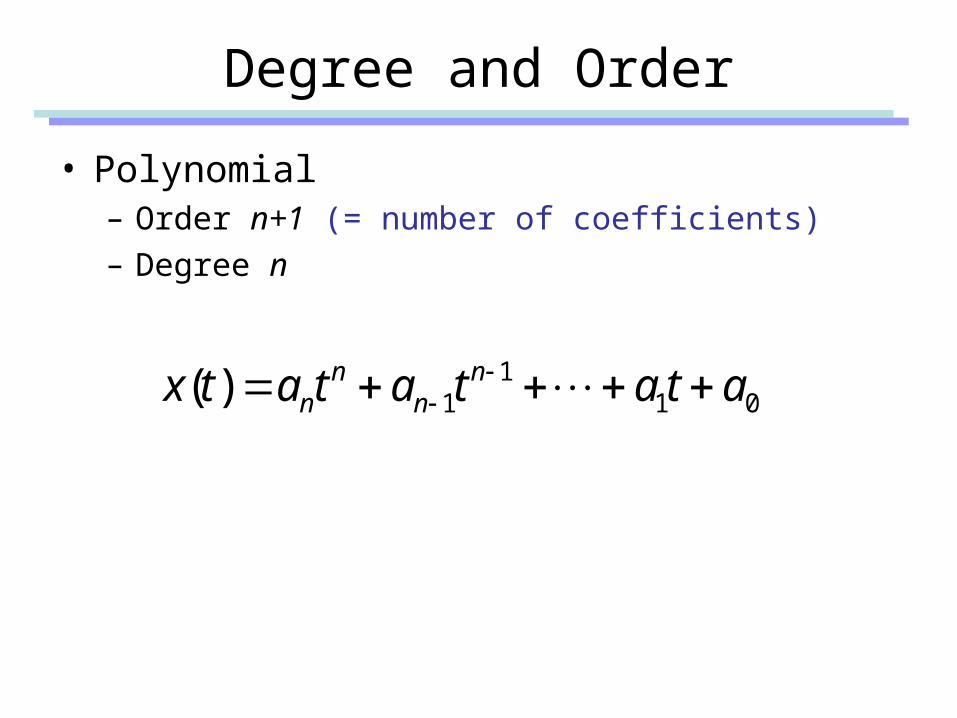
• Polynomial– Order n+1 (= number of coefficients)– Degree n
011
1)( atatatatx nn
nn
Polynomial Interpolation
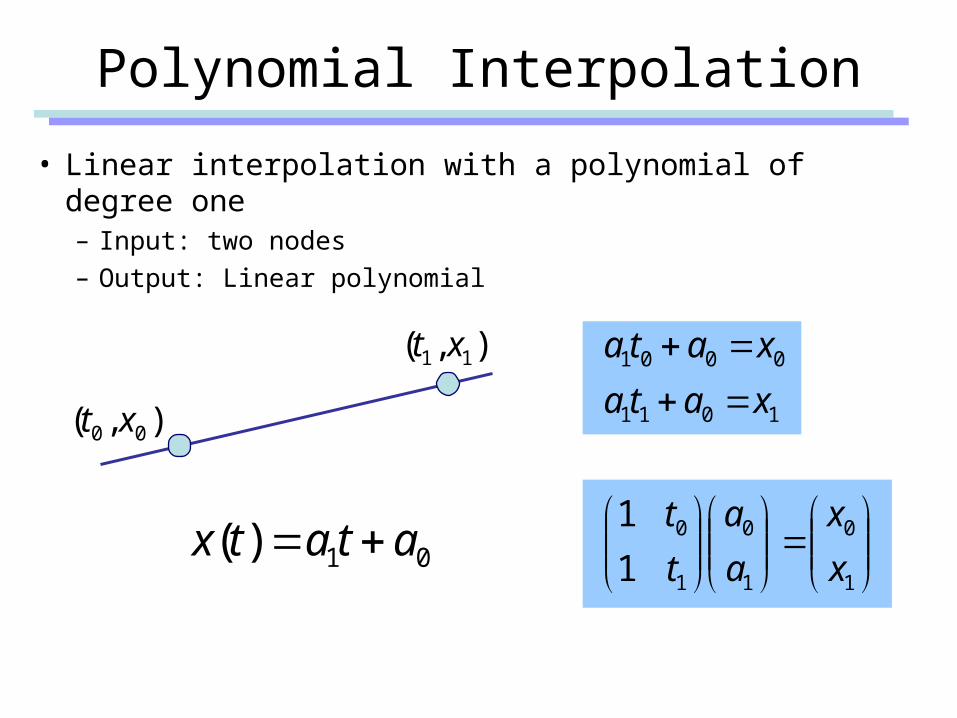
• Linear interpolation with a polynomial of degree one– Input: two nodes– Output: Linear polynomial
),( 00 xt
),( 11 xt
01)( atatx
1
0
1
0
1
0
1011
0001
1
1
x
x
a
a
t
t
xata
xata
Polynomial Interpolation
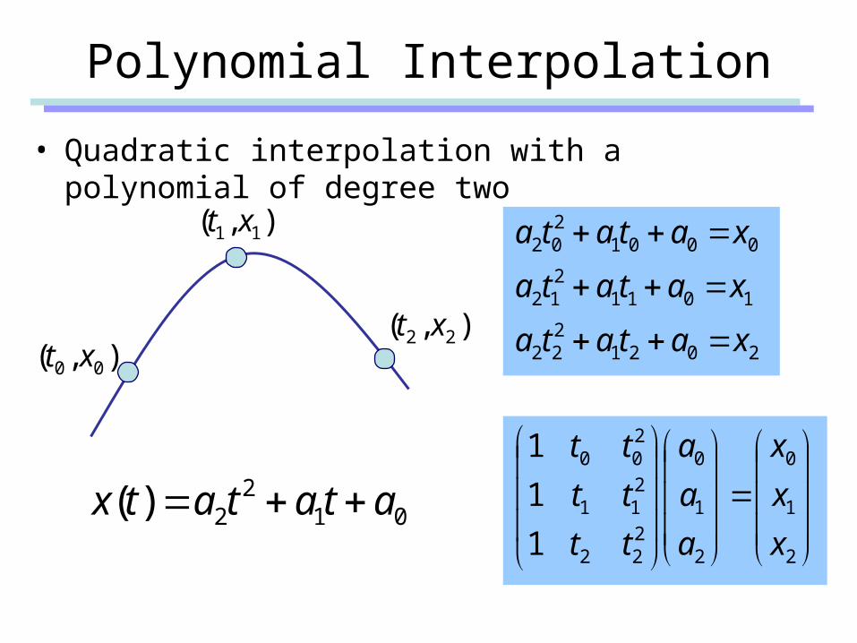
• Quadratic interpolation with a polynomial of degree two
),( 00 xt
),( 11 xt
012
2)( atatatx
2
1
0
2
1
0
222
211
200
2021222
1011212
0001202
1
1
1
x
x
x
a
a
a
tt
tt
tt
xatata
xatata
xatata
),( 22 xt

Polynomial Interpolation
• Polynomial interpolation of degree n
),( 00 xt
),( 11 xt
01)( atatatx nn
nnnn
nn
nn
nn
x
x
x
a
a
a
tt
tt
tt
1
0
1
0
1
11
1
01
0
1
1
1),( nn xt
Do we really need to solve the linear system ?
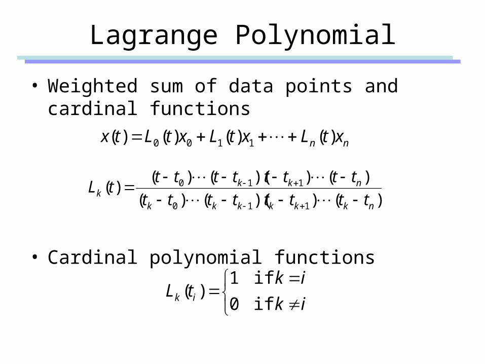
Lagrange Polynomial
• Weighted sum of data points and cardinal functions
• Cardinal polynomial functions
)())(()(
)())(()()(
110
110
nkkkkkk
nkkk tttttttt
tttttttttL
nn xtLxtLxtLtx )()()()( 1100
ik
iktL ik if0
if1)(

Limitation of Polynomial Interpolation
• Oscillations at the ends– Nobody uses higher-order polynomial interpolation now
• Demo– Lagrange.htm
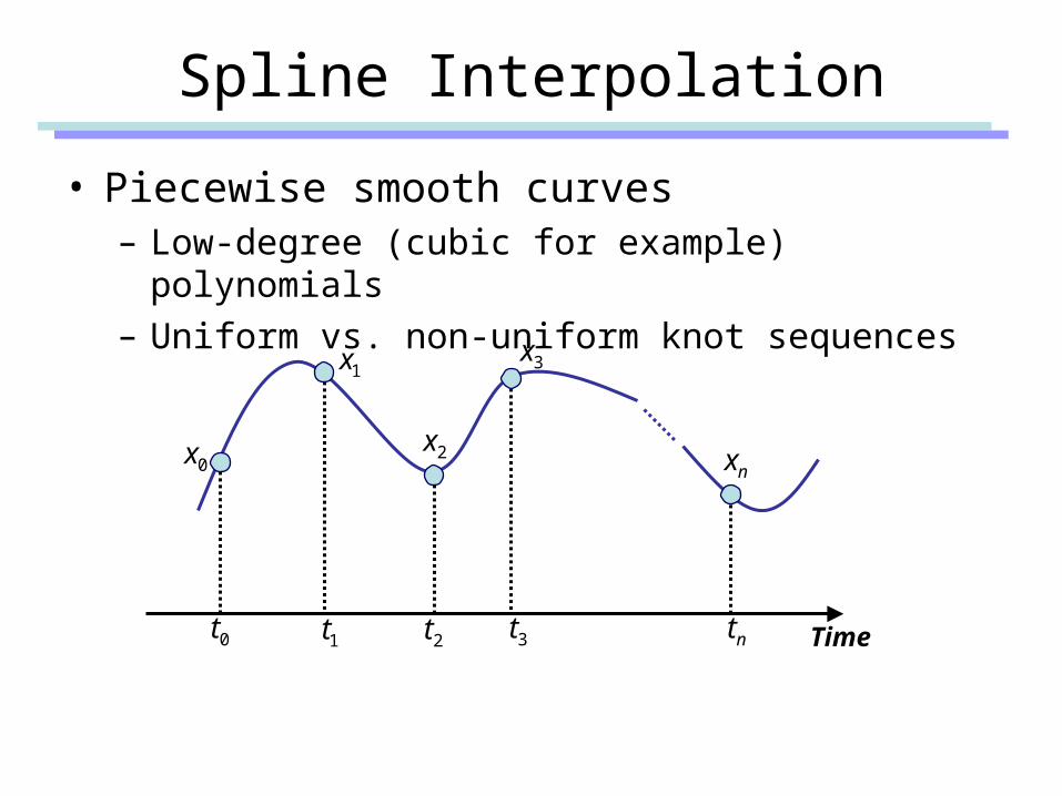
Spline Interpolation
• Piecewise smooth curves– Low-degree (cubic for example) polynomials– Uniform vs. non-uniform knot sequences
0x
1x
nx2x
3x
Time0t 1t 2t 3t nt

Why cubic polynomials ?
• Cubic (degree of 3) polynomial is a lowest-degree polynomial representing a space curve
• Quadratic (degree of 2) is a planar curve– Eg). Font design
• Higher-degree polynomials can introduce unwanted wiggles
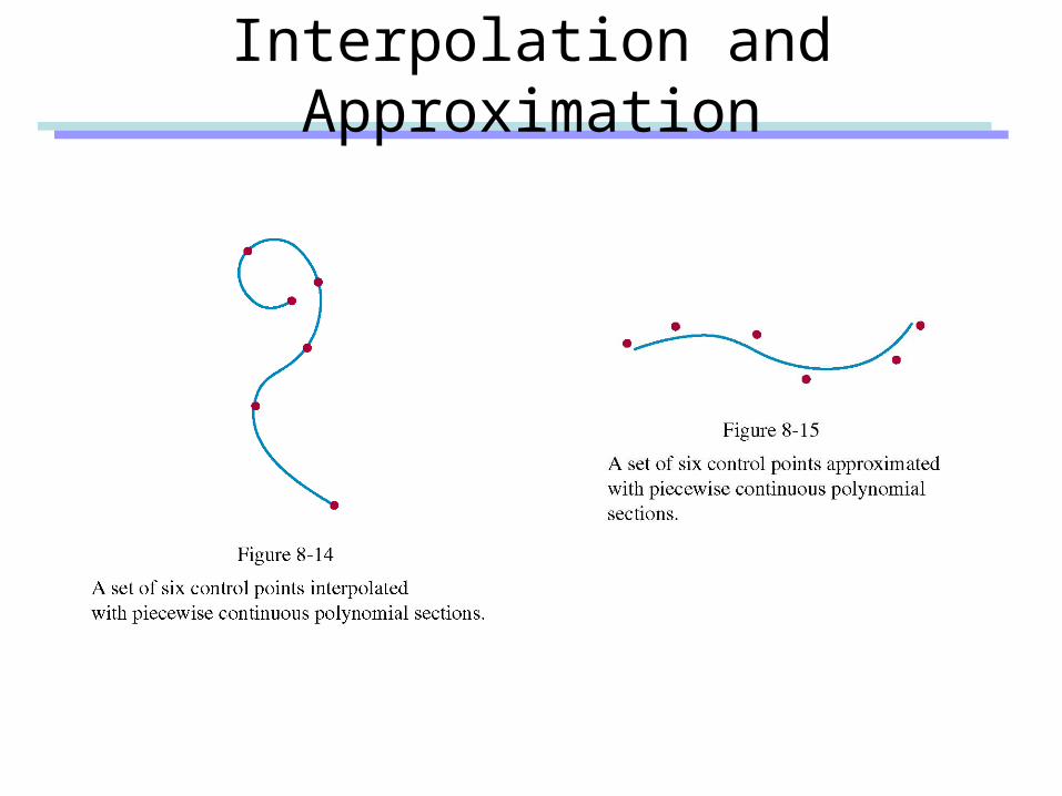
Interpolation and Approximation
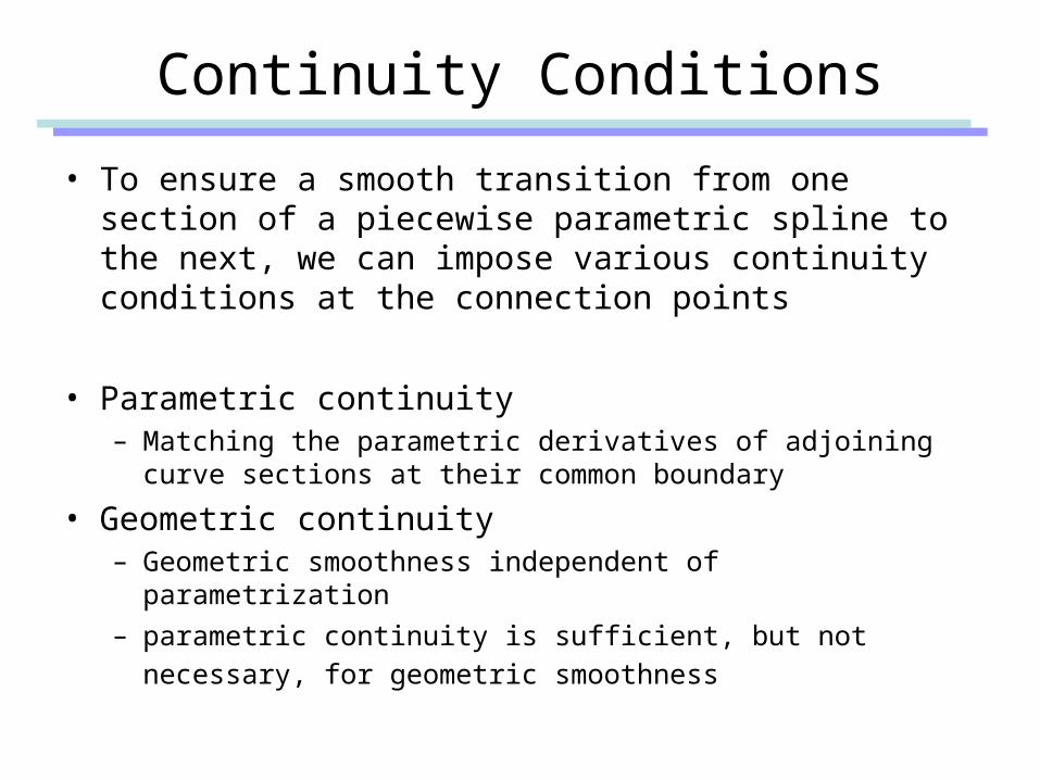
Continuity Conditions
• To ensure a smooth transition from one section of a piecewise parametric spline to the next, we can impose various continuity conditions at the connection points
• Parametric continuity– Matching the parametric derivatives of adjoining curve sections
at their common boundary
• Geometric continuity– Geometric smoothness independent of parametrization
– parametric continuity is sufficient, but not necessary, for
geometric smoothness

Parametric Continuity
• Zero-order parametric continuity– -continuity– Means simply that the curves meet
• First-order parametric continuity– -continuity– The first derivatives of two adjoining
curve functions are equal
• Second-order parametric continuity– -continuity– Both the first and the second
derivatives of two adjoining curve functions are equal
0C
1C
2C
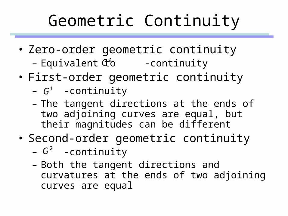
Geometric Continuity
• Zero-order geometric continuity– Equivalent to -continuity
• First-order geometric continuity– -continuity– The tangent directions at the ends of two adjoining
curves are equal, but their magnitudes can be different
• Second-order geometric continuity– -continuity– Both the tangent directions and curvatures at the
ends of two adjoining curves are equal
0C
1G
2G
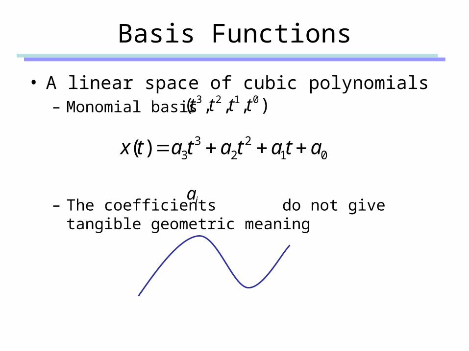
Basis Functions
• A linear space of cubic polynomials – Monomial basis
– The coefficients do not give tangible geometric meaning
012
23
3)( atatatatx
),,,( 0123 tttt
ia

Bezier Curve
• Bernstein basis functions
• Cubic polynomial in Bernstein bases
iinni tt
i
ntB
)1()(
33
22
12
03
333
322
311
300
)1(3)1(3)1(
)()()()()(
bbbb
bbbbp
tttttt
tBtBtBtBt
333
1232
231
330
)(
)1(3)(
)1(3)(
)1()(
ttB
tttB
tttB
ttB
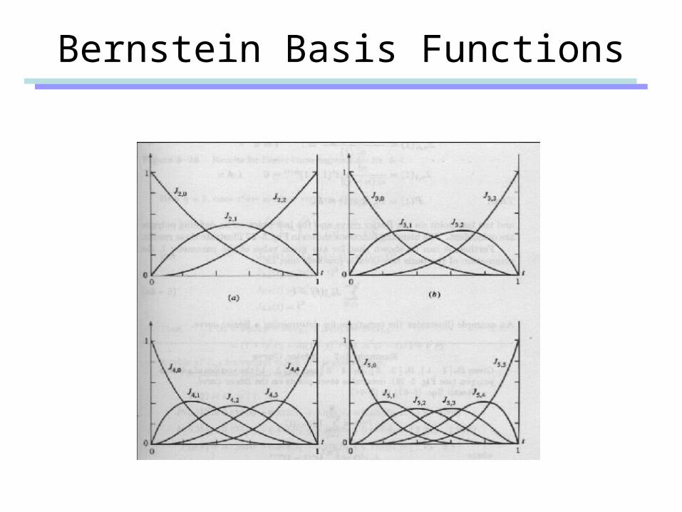
Bernstein Basis Functions

Bezier Control Points
• Control points (control polygon)
• Demo– Bezier.htm
3210 ,,, bbbb
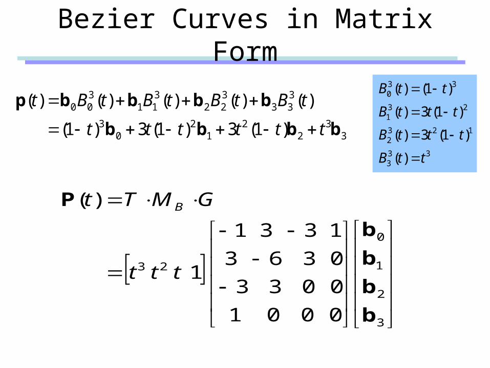
Bezier Curves in Matrix Form
3
2
1
0
23
0 0 0 1
0 0 3 3
0 3 6 3
1 3 3 1
1
)(
b
b
b
b
P
ttt
GMTt B
333
1232
231
330
)(
)1(3)(
)1(3)(
)1()(
ttB
tttB
tttB
ttB
33
22
12
03
333
322
311
300
)1(3)1(3)1(
)()()()()(
bbbb
bbbbp
tttttt
tBtBtBtBt

De Casteljau Algorithm
• Subdivision of a Bezier Curve into two curve segments

Properties of Bezier Curves
• Invariance under affine transformation– Partition of unity of Bernstein basis functions
• The curve is contained in the convex hull of the control polygon
• Variation diminishing– the curve in 2D space does not oscillate about
any straight line more often than the control point polygon
10if1)(0 ttBni

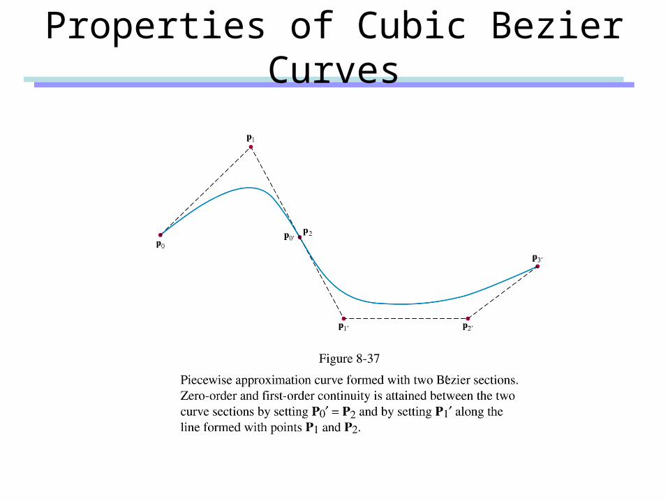
Properties of Cubic Bezier Curves
• End point interpolation
• The tangent vectors to the curve at the end points are coincident with the first and last edges of the control point polygon
)(3)1('
)(3)0('
23
01
bbp
bbp
0b
1b
2b
3b
3
0
)1(
)0(
bp
bp
Properties of Cubic Bezier Curves
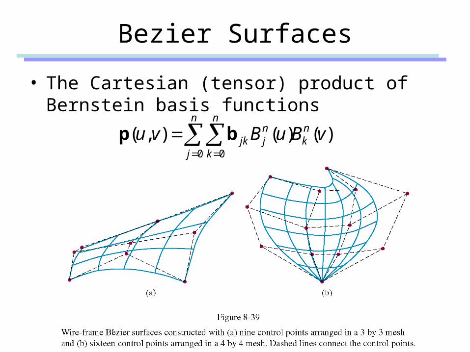
Bezier Surfaces
• The Cartesian (tensor) product of Bernstein basis functions
)()(),(0 0
vBuBvu nk
n
j
n
k
njjk
bp

Bezier Surface in Matrix Form
10 0 0 1
0 0 3 3
0 3 6 3
1 3 3 1
0 0 0 1
0 0 3 3
0 3 6 3
1 3 3 1
1
)()(),(
2
3
33231303
32221202
31211101
30201000
23
0 0
v
v
v
bbbb
bbbb
bbbb
bbbb
uuu
vBuBvu
TT
nk
n
j
n
k
njjk
VMGMU
bp
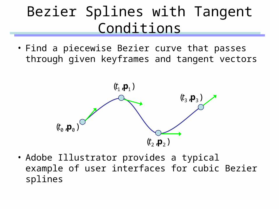
Bezier Splines with Tangent Conditions
• Find a piecewise Bezier curve that passes through given keyframes and tangent vectors
• Adobe Illustrator provides a typical example of user interfaces for cubic Bezier splines
),( 00 pt
),( 11 pt
),( 22 pt
),( 33 pt

Catmull-Rom Splines
• Polynomial interpolation without tangent conditions– -continuity– Local controllability
• Demo– CatmullRom.html
),( 00 pt
),( 11 pt
),( 22 pt
),( 33 pt
2)(' 11 ii
itpp
p
1C

Natural Cubic Splines
• Is it possible to achieve higher continuity ?– -continuity can be achieved from splines of
degree n
• Motivated by loftman’s spline– Long narrow strip of wood or plastic– Shaped by lead weights (called ducks)
1nC
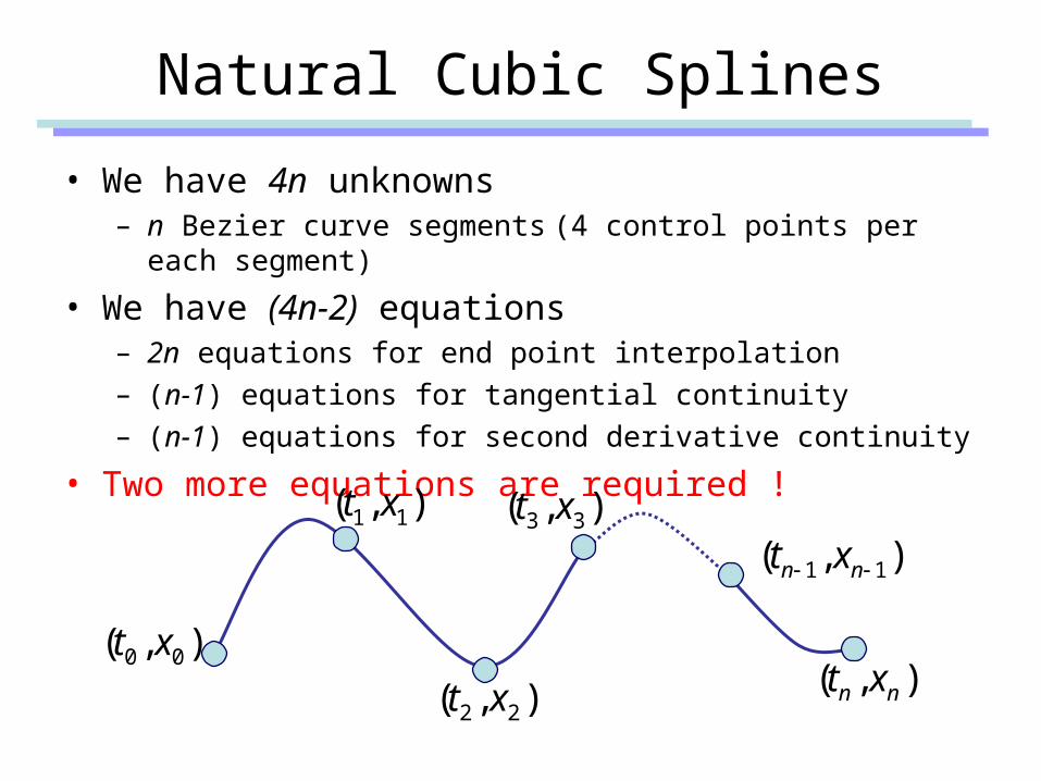
Natural Cubic Splines
• We have 4n unknowns – n Bezier curve segments (4 control points per each segment)
• We have (4n-2) equations– 2n equations for end point interpolation– (n-1) equations for tangential continuity– (n-1) equations for second derivative continuity
• Two more equations are required !
),( 00 xt
),( 11 xt
),( nn xt),( 22 xt
),( 33 xt),( 11 nn xt

Natural Cubic Splines
• Natural spline boundary condition
• Closed boundary condition
• High-continuity, but no local controllability
• Demo– natcubic.html
– natcubicclosed.html
0)()( 0 ntxtx
)()(and)()( 00 nn txtxtxtx

B-splines
• Is it possible to achieve both -continuity and local controllability ?– B-splines can do !– But, B-splines do not interpolate any of control points
• Uniform cubic B-spline basis functions
333
2332
2331
330
6
1)(
)1333(6
1)(
)463(6
1)(
)1(6
1)(
ttB
ttttB
tttB
ttB
2C
)()()()(
)()(
333
322
311
300
3
0
3
tBtBtBtB
tBtj
jj
bbbb
bp
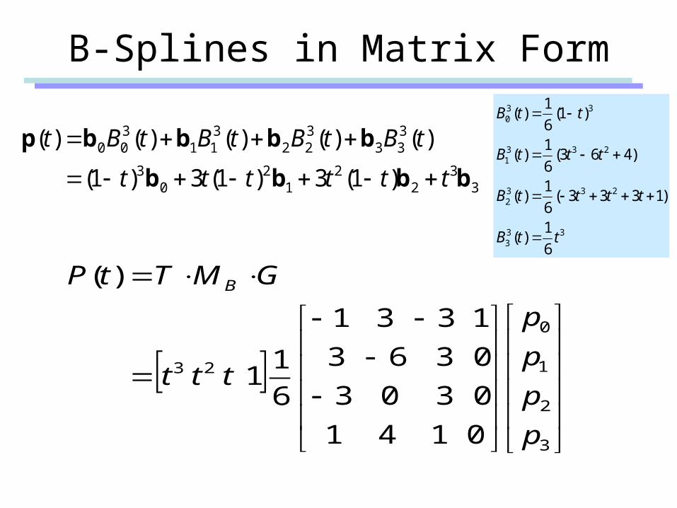
B-Splines in Matrix Form
3
2
1
0
23
0 1 4 1
0 3 0 3
0 3 6 3
1 3 3 1
6
11
)(
p
p
p
p
ttt
GMTtP B
33
22
12
03
333
322
311
300
)1(3)1(3)1(
)()()()()(
bbbb
bbbbp
tttttt
tBtBtBtBt
333
2332
2331
330
6
1)(
)1333(6
1)(
)463(6
1)(
)1(6
1)(
ttB
ttttB
tttB
ttB

Uniform B-spline basis functions
• Bell-shaped basis function for each control points
• Overlapping basis functions– Control points correspond to knot points

B-spline Properties
• Convex hull• Affine invariance• Variation diminishing• -continuity• Local controllability
• Demo– Bspline.html
2C

NURBS
• Non-uniform Rational B-splines– Non-uniform knot spacing– Rational polynomial
• A polynomial divided by a polynomial• Can represent conics (circles, ellipses, and hyperbolics)• Invariant under projective transformation
• Note– Uniform B-spline is a special case of non-uniform B-spline– Non-rational B-spline is a special case of rational B-spline
n
j
njj
n
j
njjj
tB
tB
t
0
0
)(
)(
)(
bp
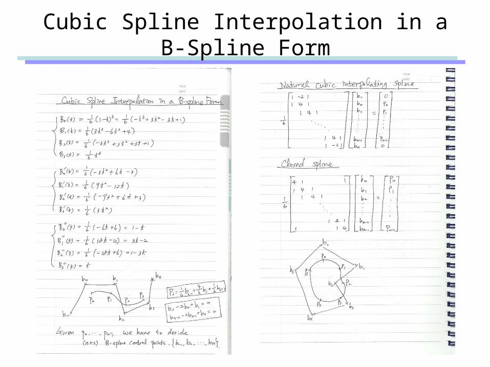
Cubic Spline Interpolation in a B-Spline Form
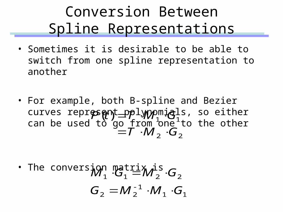
Conversion BetweenSpline Representations
• Sometimes it is desirable to be able to switch from one spline representation to another
• For example, both B-spline and Bezier curves represent polynomials, so either can be used to go from one to the other
• The conversion matrix is
22
11)(
GMT
GMTtP
111
22
2211
GMMG
GMGM

Displaying Spline Curves
• Forward-difference calculation– Generate successive values recursively by
incrementing previously calculated values– For example, consider a cubic polynomial
– We want to calculate x(t) at tk for k=0,1,2,…
dctbtattx 23)(
kk tt 1

Displaying Spline Curves
• Forward-difference calculation– Two successive values of a cubic polynomial
– The forward difference is a quadratic polynomial with respect to t
dtctbtatx
dctbtattx
kkkk
kkkk
)()()()(
)(23
1
23
)()23(3
)()()(2322
1
cbatbata
txtxtx
kk
kkk
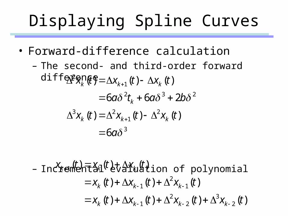
Displaying Spline Curves
• Forward-difference calculation– The second- and third-order forward difference
– Incremental evaluation of polynomial
3
21
23
232
12
6
)()()(
266
)()()(
a
txtxtx
bata
txtxtx
kkk
k
kkk
)()()()(
)()()(
)()()(
23
22
1
12
1
1
txtxtxtx
txtxtx
txtxtx
kkkk
kkk
kkk

Matrix Equations for B-splines
• Cubic B-spline curves
333
2332
2331
330
6
1)(
)1333(6
1)(
)463(6
1)(
)1(6
1)(
ttB
ttttB
tttB
ttB
3
2
1
0
32
3
2
1
0
32
3
2
1
0
33
32
31
30
333
322
311
300
1
1331
0363
0303
0141
6
11
)()()()(
)()()()()(
p
p
p
p
p
p
p
p
p
p
p
p
ppppp
Mtttttt
tBtBtBtB
tBtBtBtBt
Control PointsGeometric Matrix
Monomial Bases

Curve Refinement
• Subdivide a curve into two segments• Figures and equations were taken from
http://graphics.idav.ucdavis.edu/education/CAGDNotes/homepage.html
Binary Subdivision
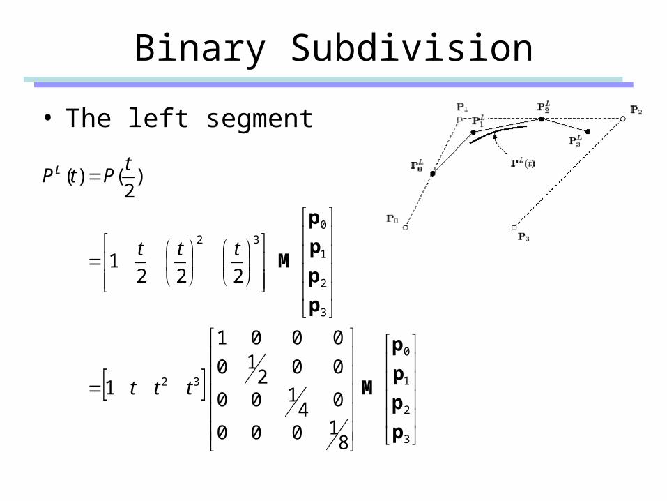
• The left segment
3
2
1
0
32
3
2
1
032
81000
04100
00210
0001
1
2221
)2
()(
p
p
p
p
M
p
p
p
p
M
ttt
ttt
tPtPL
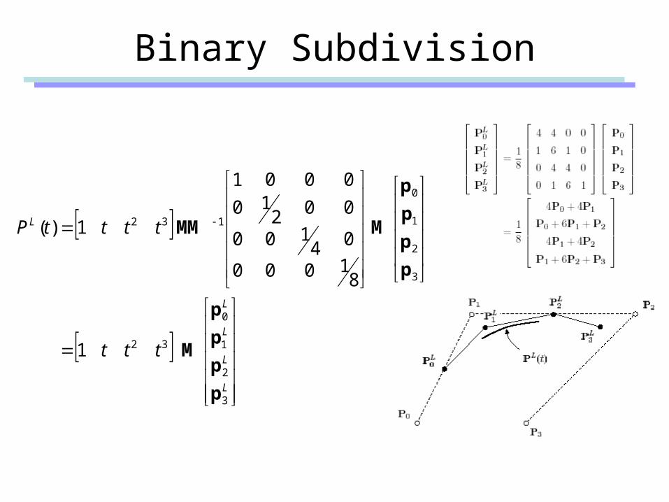
Binary Subdivision
L
L
L
L
L
ttt
ttttP
3
2
1
0
32
3
2
1
0
132
1
81000
04100
00210
0001
1)(
p
p
p
p
M
p
p
p
p
MMM
Binary Subdivision

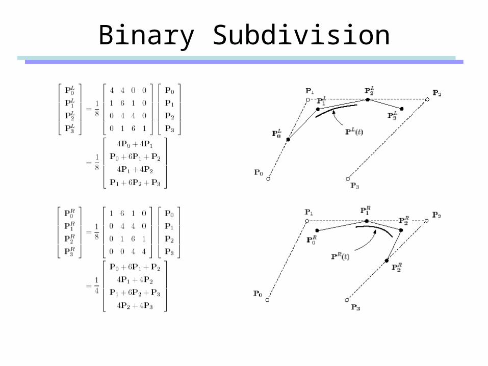
The Subdivision Rule for Cubic B-Splines
• The new control polygon consists of– Edge points: the midpoints of the line segments– Vertex points: the weighted average of the
corresponding vertex and its two neighbors

Recursive Subdivision
• Recursive subdivision brings the control polygon to converge to a cubic B-spline curve
• Control polygon + subdivision rule– Yet another way of defining a smooth curve
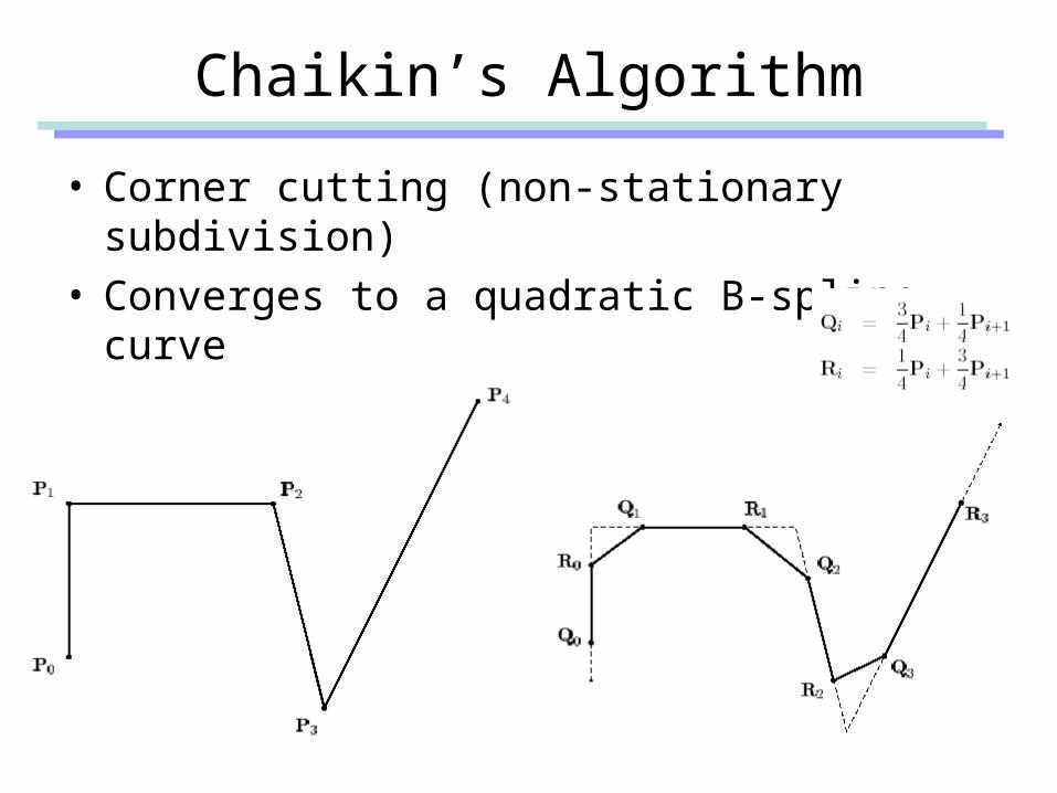
Chaikin’s Algorithm
• Corner cutting (non-stationary subdivision)• Converges to a quadratic B-spline curve• Demo: subdivision.htm
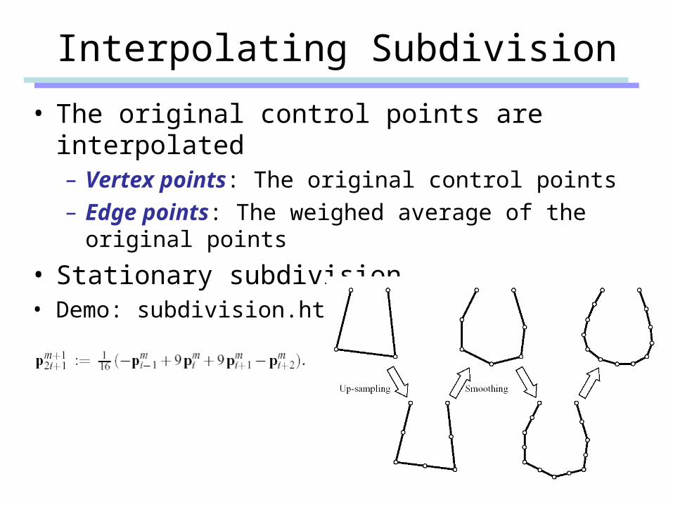
Interpolating Subdivision
• The original control points are interpolated– Vertex points: The original control points– Edge points: The weighed average of the original points
• Stationary subdivision• Demo: subdivision.htm
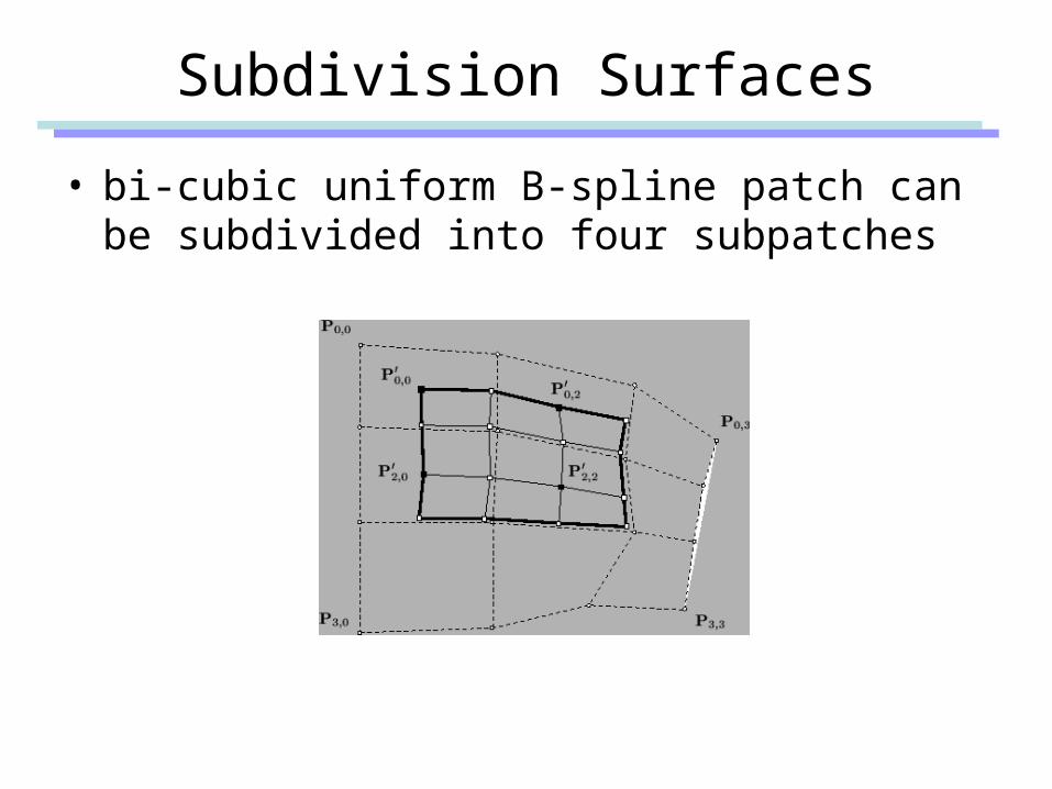
Subdivision Surfaces
• bi-cubic uniform B-spline patch can be subdivided into four subpatches
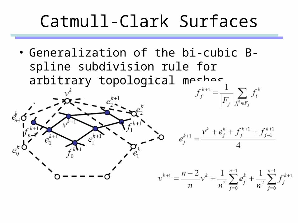
Catmull-Clark Surfaces
• Generalization of the bi-cubic B-spline subdivision rule for arbitrary topological meshes

Catmull-Clark Surfaces

Subdivision in Action
• A Bug’s Life

Subdivision in Action
• Geri’s Game

Summary
• Polynomial interpolation– Lagrange polynomial
• Spline interpolation– Piecewise polynomial– Knot sequence– Continuity across knots
• Natural spline ( -continuity)• Catmull-Rom spline ( -continuity)
– Basis function• Bezier• B-spline
2C1C