Motion Blending(Multidimensional Interpolation)

Jehee Lee

Data-Driven Approach

• It is difficult to understand basic principles of the real world– Instead, we would like to sample the real world !

• What kind of data is available ?– Pictures (camera), video (camcorder)– Motion, facial expression (motion capture)– Geometry (3D scanner)– Voice, sound (recorder)– Tactile, physical properties, …

• Data-driven approaches try to reconstruct the real world in a computer from a rich set of samples

The real world is multi-dimensional

• Simple (object space) classification– One dimension: Sketch, curve– Two dimension: Pictures, surface, tactile– Three dimension: 3D geometry, video– Four dimension: Particle motion (position + time)– High dimension: Articulated figure motion

• Many interpretations (parameterizations) are possible independent of object space dimensions

Dimensionality of Motion

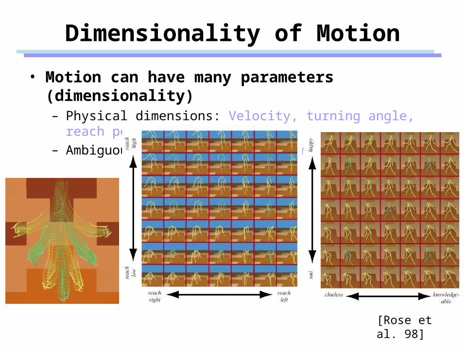
• Motion can have many parameters (dimensionality)– Physical dimensions: Velocity, turning angle, reach position– Ambiguous dimensions: Style, emotion, mood

[Rose et al. 98]

The Space of Motion

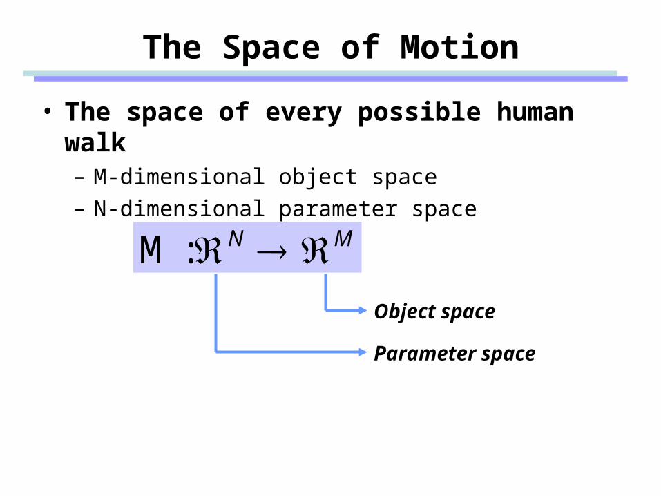
• The space of every possible human walk– M-dimensional object space– N-dimensional parameter space

MN :M

Object space

Parameter space

Multi-Dimensional Interpolation

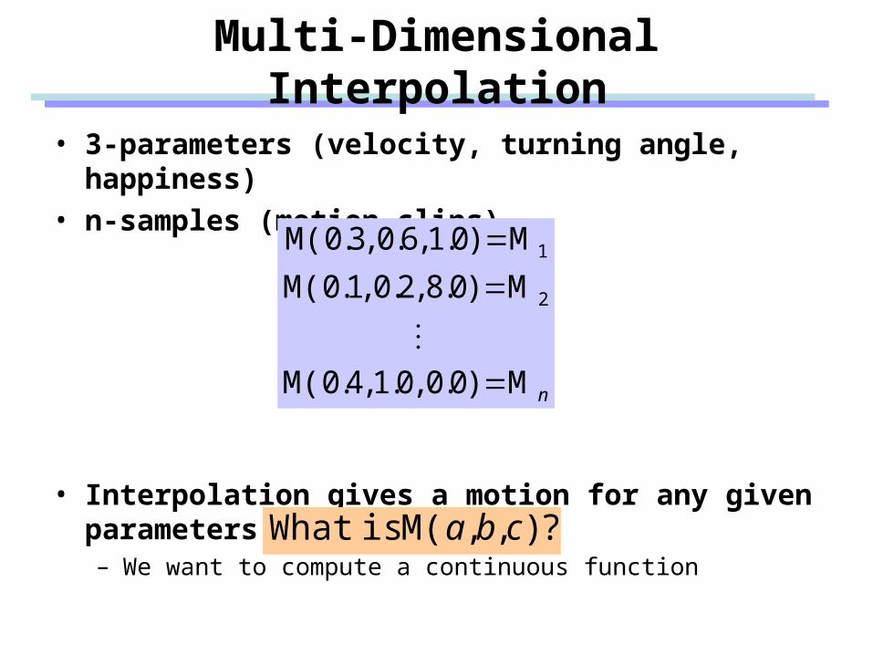
• 3-parameters (velocity, turning angle, happiness)• n-samples (motion clips)

• Interpolation gives a motion for any given parameters– We want to compute a continuous function

nM)0.0,0.1,4.0M(

M)0.8,2.0,1.0M(

M)0.1,6.0,3.0M(

2

1

? ),,M( isWhat cba

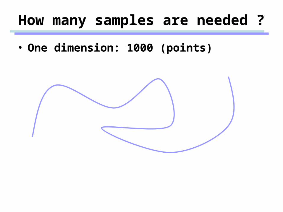
How many samples are needed ?

• One dimension: 1000 (points)

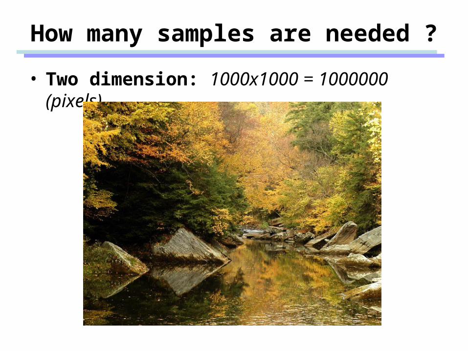
How many samples are needed ?

• Two dimension: 1000x1000 = 1000000 (pixels)

How many samples are needed ?

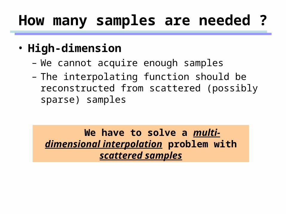
• High-dimension– We cannot acquire enough samples– The interpolating function should be reconstructed

from scattered (possibly sparse) samples

We have to solve a multi-dimensional interpolation problem with scattered samples

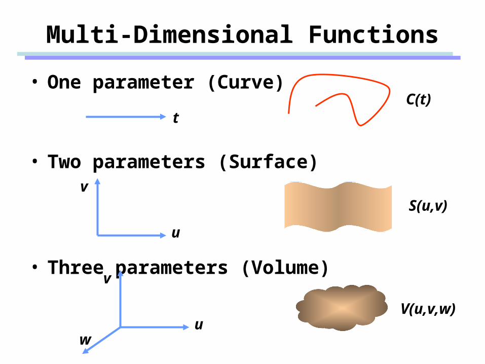
Multi-Dimensional Functions

• One parameter (Curve)

• Two parameters (Surface)

• Three parameters (Volume)

t

u

v

u

v

w

C(t)

S(u,v)

V(u,v,w)

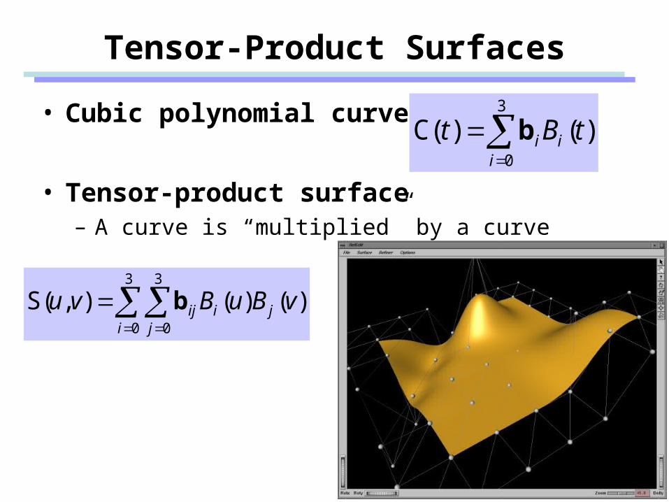
Tensor-Product Surfaces

• Cubic polynomial curve

• Tensor-product surface– A curve is “multiplied” by a curve

3

0

)()C(i

ii tBt b

3

0

3

0

)()(),S(i j

jiij vBuBvu b

Tensor-Product Functions

• Tensor-product is a standard technique for increasing the dimension of parametric functions– Bezier surfaces, B-spline surfaces, NURBS surfaces, …

• It works fine for low-dimensional parametric spaces– Great for surfaces– Maybe good enough for volumes

• It can be problematic for higher-dimensions– Too many control points– High degree of basis functions

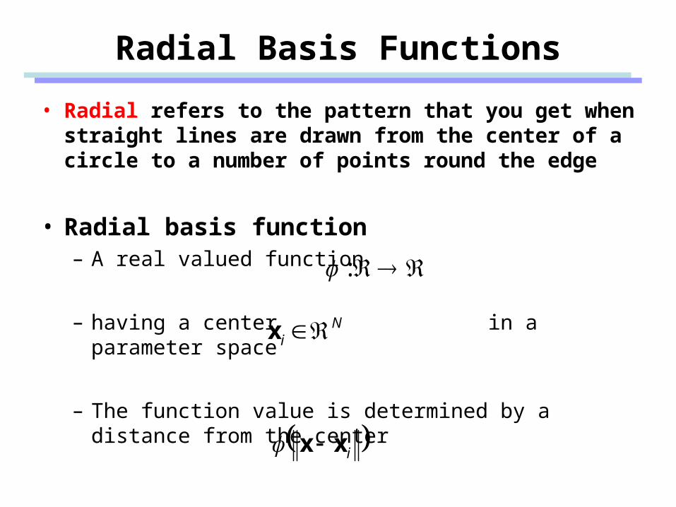
Radial Basis Functions

• Radial refers to the pattern that you get when straight lines are drawn from the center of a circle to a number of points round the edge

• Radial basis function – A real valued function

– having a center in a parameter space

– The function value is determined by a distance from the center

:

Ni x

ixx

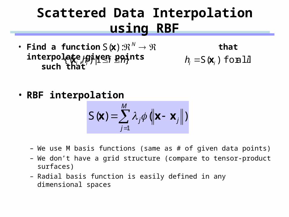
Scattered Data Interpolation using RBF

• Find a function that interpolate given points such that

• RBF interpolation

– We use M basis functions (same as # of given data points)– We don’t have a grid structure (compare to tensor-product

surfaces)– Radial basis function is easily defined in any dimensional spaces

N:)S(x}1|),{( nihii x ih ii allfor )S(x

M

jjj

1

)()S( xxx

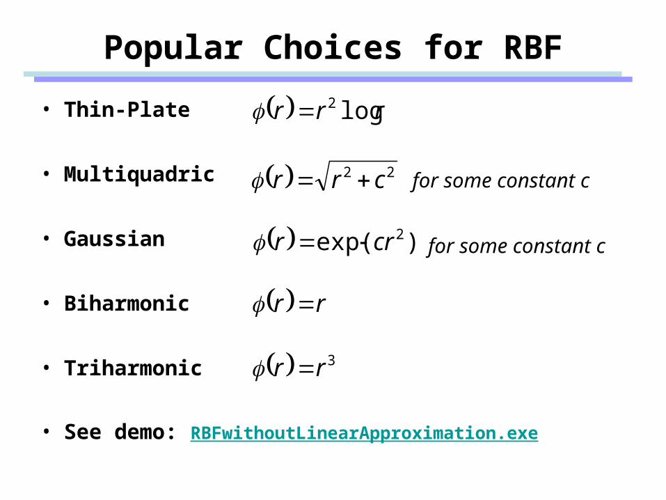
Popular Choices for RBF

• Thin-Plate

• Multiquadric

• Gaussian

• Biharmonic

• Triharmonic

• See demo: RBFwithoutLinearApproximation.exe

rrr log2

22 crr

rr

3rr

)exp( 2crr

for some constant c

for some constant c

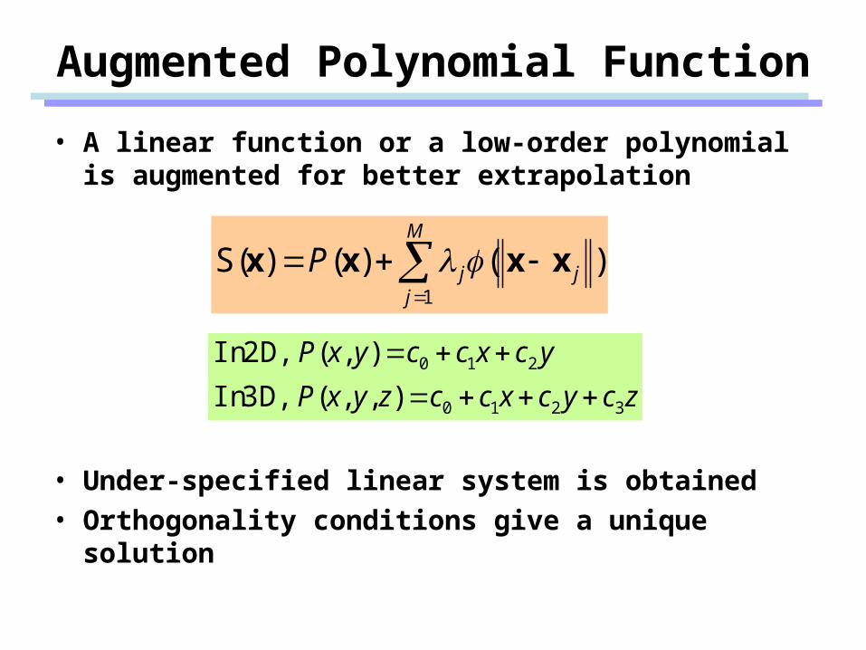
Augmented Polynomial Function

• A linear function or a low-order polynomial is augmented for better extrapolation

• Under-specified linear system is obtained• Orthogonality conditions give a unique solution

M

jjjP

1

)()()S( xxxx

zcycxcczyxP

ycxccyxP

3210

210

),,( 3D,In

),( 2D,In

Motion Blending

• S. I. Park, et al., On-line Locomotion Generation Based on Motion Blending, Symposium on Computer Animation, 2002

• Movie

Application to Motion Blending

• The length of time– The first motion is 3 seconds long, the second motion

is 5 seconds long, and so on.– Those motions are normalized in time and blended– What is the length of the blend ?

• The length of the blend can be negative– RBF interpolation doesn’t have convex hull property– Is it make sense to create a “backward walk” by

blending “forward walks” ?

Application to Motion Blending

• Handling unit quaternions (or rotation matrices)– What if we apply RBF interpolation component-wisely ?

• Represent the surface as an affine combination– Construct cardinal basis functions using RBF

Application to Motion Blending

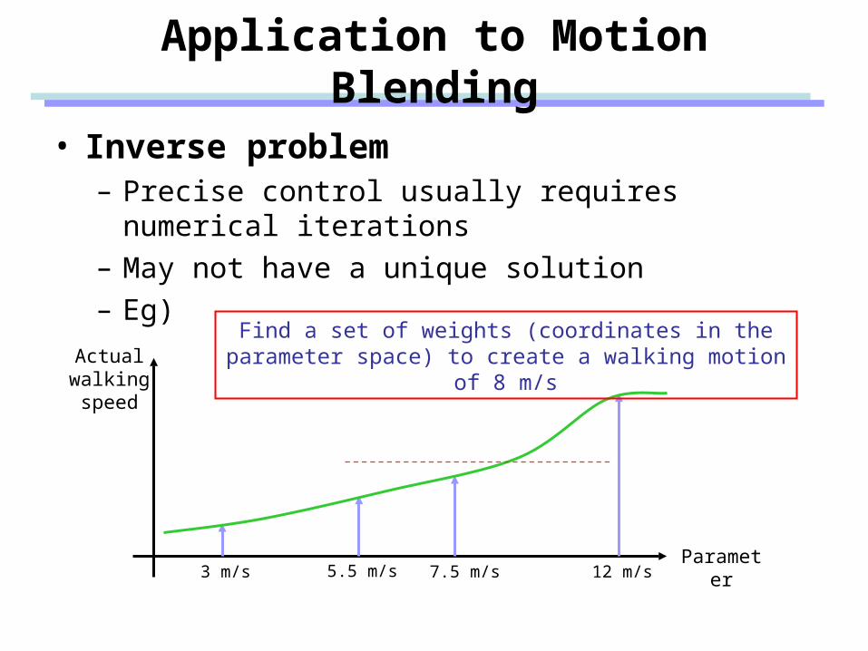
• Inverse problem– Precise control usually requires numerical iterations– May not have a unique solution– Eg)

Parameter3 m/s 5.5 m/s 7.5 m/s 12 m/s

Find a set of weights (coordinates in the parameter space) to create a walking motion of 8 m/sActual

walking speed

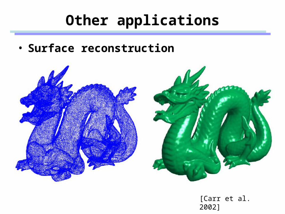
Other applications

• Surface reconstruction

[Carr et al. 2002]

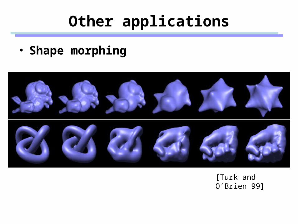
Other applications

• Shape morphing

[Turk and O’Brien 99]

Summary

• Multidimensional interpolation– Sparse samples in high-dimensional spaces– Time-series data

• Scatter data interpolation using radial basis functions– The basis function is determined by applications– All basis function explained are not locally supported– For some applications, locally supported basis functions should

be chosen