Spline Adaptation in Extended Linear ModelsMark H. Hansen and Charles Kooperberg 1Abstract. In many statistical applications, nonparametric modeling can provide insight into thefeatures of a dataset that are not obtainable by other means. One successful approach involvesthe use of (univariate or multivariate) spline spaces. As a class, these methods have inheritedmuch from classical tools for parametric modeling. For example, stepwise variable selection withspline basis terms is a simple scheme for locating knots (breakpoints) in regions where the dataexhibit strong, local features. Similarly, candidate knot con�gurations (generated by this orsome other search technique), are routinely evaluated with traditional selection criteria like AICor BIC. In short, strategies typically applied in parametric model selection have proved useful inconstructing exible, low-dimensional models for nonparametric problems.Until recently, greedy, stepwise procedures were most frequently suggested in the literature.Research into Bayesian variable selection, however, has given rise to a number of new spline-basedmethods that primarily rely on some form of Markov chain Monte Carlo to identify promisingknot locations. In this paper, we consider various alternatives to greedy, deterministic schemes,and present a Bayesian framework for studying adaptation in the context of an extended linearmodel (ELM). Our major test cases are Logspline density estimation and (bivariate) Triogramregression models. We selected these because they illustrate a number of computational andmethodological issues concerning model adaptation that arise in ELMs.Key Words and phrases: Adaptive triangulations; AIC; Density estimation; Extended linearmodels; Finite elements; Free knot splines; GCV; Linear splines; Multivariate splines; Regression.1. IntroductionPolynomial splines are at the heart of many popular techniques for nonparametric function estimation. Forregression problems, TURBO (Friedman and Silverman, 1989), multivariate adaptive regression splines orMARS (Friedman, 1991) and � (Breiman, 1991) have all met with considerable success. In the context ofdensity estimation, the Logspline procedure of Kooperberg and Stone (1991, 1992) exhibits excellent spatialadaptation, capturing the full height of spikes without over�tting smoother regions. And �nally, amongclassi�cation procedures, classi�cation and regression trees or CART (Breiman et al. 1984) is a de factostandard, while the more recent PolyMARS models (Kooperberg et al. 1997) have been able to tackle evenlarge problems in speech recognition. Stone et al. (1997) and a forthcoming monograph by Hansen, Huang,Kooperberg, Stone and Truong are the prime references for the application of polynomial splines to functionestimation. In this paper, we review a general methodological framework common to procedures like MARSand Logspline, and contrast it with several Bayesian approaches to spline modeling. We begin with somebackground material on splines.1Mark H. Hansen is a Member of the Technical Sta�, Bell Laboratories, Murray Hill, NJ 07974. Charles Kooperberg isAssociate Member, Division of Public Health Sciences, Fred Hutchinson Cancer Research Center, Seattle, WA 98109-1024.

1.1 SplinesUnivariate, polynomial splines are piecewise polynomials of some degree d. The breakpoints marking atransition from one polynomial to the next are referred to as knots. In this paper, we will let the vectort = (t1; : : : ; tK) 2 RK denote a collection of K knots. Typically, a spline will also satisfy smoothnessconstraints describing how the di�erent pieces are to be joined. These restrictions are speci�ed in termsof the number of continuous derivatives, s, exhibited by the piecewise polynomials. Consider, for example,piecewise linear curves. Without any constraints, these functions can have discontinuities at the knots. Byadding the condition that the functions be globally continuous, we force the separate linear pieces to meetat each knot. If we demand even greater smoothness (say, continuous �rst derivatives), we loose exibilityat the knots and the curves become simple linear functions. In the literature on approximation theory,the term \linear spline" is applied to a continuous, piecewise linear function. Similarly, the term \cubicspline" is reserved for piecewise cubic functions having two continuous derivatives, allowing jumps in thethird derivatives at the knots. In general, it is common to work with splines having maximal smoothness inthe sense that any more continuity conditions would result in a global polynomial.Given a degree d and a knot vector t, the collection of polynomial splines having s continuous derivativesforms a linear space. For example, the collection of linear splines with knot sequence t is spanned by thefunctions 1; x; (x� t1)+; : : : ; (x� tK)+ (1)where (�)+ = max(�; 0). We refer to this set as the truncated power basis of the space. In general, the basisfor a spline space of degree d and smoothness s is made up of monomials up to degree d together with termsof the form (x � tk)s+j+ , where 1 � j � d� s. Using this formula the classical cubic splines have d = 3 ands = 2 so that the basis has elements1; x; x2; x3; (x� t1)3+; : : : ; (x� tk)3+ : (2)From a modeling standpoint, the truncated power basis is convenient because the individual functions aretied to knot locations. In the expressions (1) and (2), there is exactly one function associated with eachknot, and eliminating that function e�ectively removes the knot. This observation is at the heart of manystatistical methods that involve splines and will be revisited shortly.The truncated power functions (1) and (2) are known to have rather poor numerical properties. In linearregression problems, for example, the condition of the design matrix deteriorates rapidly as the number ofknots increases. An important alternative representation is the so-called B-spline basis (de Boor, 1978).These functions are constructed to have support only on a few neighboring intervals de�ned by the knots.(For splines having maximal smoothness, this means d + 1 neighboring intervals.) A detailed descriptionof this basis is beyond the scope of this paper, but the interested reader is referred to Schumaker (1993).For the moment, assume we can �nd a basis B1(x; t); : : : ; BJ(x; t) for the space of splines of degree d withsmoothness s and knot sequence t so that any function in the space can be written asg(x;�; t) = �1B1(x; t) + � � ��JBJ(x; t) ; (3)for some coe�cient vector � = (�1; : : : ; �J)t. If we are dealing with spline spaces of maximal smoothness,then J = K + d + 1, as we have seen in (1) and (2). Given this structure, we now brie y describe abroad collection of estimation problems that admit relatively natural techniques for identifying good �ttingfunctions g. 2

1.2 Extended linear modelsExtended linear models (ELMs) were originally de�ned as a theoretical tool for understanding the propertiesof spline-based procedures in a large class of estimation problems (Hansen, 1994; Stone et al. 1997; Huang,1998, 2001). This class is extremely rich, containing all of the standard generalized linear models as well asdensity and conditional density estimation, hazard regression, censored regression, spectral density estimationand polychotomous regression. To describe an ELM, we begin with a probability model p(W jh) for a (possiblyvector-valued) random variable W that depends on an unknown (also possibly vector-valued) function h.Typically, h represents some component of the probability model about which we hope to make inferences.For example, in a normal linear model, h is the regression function; while for density estimation, we take hto be the log-density.Let l(W jh) = log p(W jh) denote the log-likelihood for an ELM, and assume that there exists a uniquefunction � that maximizes the expected log-likelihood El(W jh) over some class of functions H . The maxi-mizer � de�nes \truth," and is the target of our estimation procedures. The class H is chosen to capture ourbeliefs about �, and is commonly de�ned through smoothness conditions (e.g., we might assume that the trueregression function in a linear model has two continuous, bounded derivatives). These weak assumptionsabout � tend to result in classes H that are in�nite dimensional. Therefore, for estimation purposes wechoose to work with exible, �nite-dimensional spaces G that have good approximation properties. That is,the elements g 2 G can capture the major features of functions � 2 H , or ming2G kg � �k is small in somenorm for all � 2 H . Splines are one such approximation space.Given a series of observations W1; : : : ;Wn from the distribution of W , we estimate � by maximizing thelog-likelihood l(g) =Xi l(g;Wi) where g 2 G : (4)We refer to this set-up as an extended linear model for �. In this case, the term \linear" refers to our use of alinear space G. Our appeal to maximum likelihood in this context does not imply that we believe p(W j�) tobe the true, data-generating distribution for W . Rather, p may be chosen for simple computational ease inthe same way that ordinary least squares can be applied when the assumption of strict normality is violated.In theoretical studies, it is common to let the dimension of G depend on the sample size n. For example, ifG is a spline space with K knots, we let K = K(n)!1 as n!1. As we collect more data, we are able toentertain more exible descriptions of �. Asymptotic results describing the number of knots K(n) and theirplacement needed to achieve optimal mean squared error behavior are given in Stone (1985), Stone (1994),Hansen (1994), and Huang (1998, 2001) and Stone and Huang (2001).An ELM is said to be concave if the log-likelihood l(wjh) is concave in h for each value of w 2 W andif El(W jh) is strictly concave in h (when restricted to those h for which El(W jh) > �1). Strict concavityholds for all of the estimation problems listed at the beginning of this section. Now, let G be a spline spaceof degree d with knot sequence t so that any g 2 G can be written in the form (3). Then since g = g(�;�; t),the log-likelihood (4) can be written as l(�; t). Because of concavity, the MLEs �̂ for the coe�cients � anda �xed t can be found e�ciently in reasonably-sized problems through simple Newton-Raphson iterations.Therefore, it is possible to compute l(t) = max� l(�; t) : (5)3

After making the dependence on t explicit in this way, we can consider adjusting the knot locations t1 <� � � < tK to maximize the log-likelihood. It is intuitively clear that the knot sequence t = (t1; : : : ; tK)controls the exibility of elements in g to track local features: tightly-spaced knots can capture peaks, whilewidely-separated knots produce smooth �ts.However, even in the simplest case, linear regression with a single univariate predictor, maximizing (5)over knot sequences is a di�cult optimization problem. To see this, we �rst translate univariate regressioninto an ELM: Let W = (X;Y ) and de�ne p(W jh) via the relationshipY = h(X) + � ;for an unknown regression function h. The error � is assumed independent of X with a normal distributionhaving mean zero and variance �2. For a spline space G, the negative log-likelihood for � is proportional tothe regression sum of squaresRSS(�; t) =Xi (Yi � g(xi;�; t))2 =Xi (Yi � �1B1(Xi; t)� � � � � �JBJ (Xi; t))2 :If we hold t �xed, then l(t) / max� f�RSS(�; t)g = �RSS(�̂; t) ; (6)where �̂ is the ordinary least squares estimate of �. Jupp (1978) demonstrated that �RSS(t) has localmaxima along lines of the form tk = tk+1, making the solution to (6) di�cult for standard optimizationsoftware. Not surprisingly, this problem persists in even more exotic ELMs.Several authors have considered special transformations, penalties or ad hoc optimization schemes tomaximize the log-likelihood with respect to t (Jupp, 1978; Lindstrom, 1999; Kooperberg and Stone, 2001).In this paper, we will instead consider an approximate solution that begins by connecting knot placementwith model selection.1.3 Model selectionThe concavity of an ELM together with the association of knot locations to terms in the truncated power basissuggests simple approximations to maximizing (5) based on fast, stepwise approaches to model selection.Consider splines of degree d having maximal smoothness and knot sequence t. According to Section 1.1, thismeans that s = d � 1 and each knot point tk in t is associated with only one of the truncated monomials(x� tk)d+; the linear (1) and cubic (2) splines are two examples. Therefore, moving tk e�ects only one basiselement in G, and in fact removing tk entirely is equivalent to deleting (x � tk)d+ from the model. Manyexisting spline methods use this idea in some form. It was originally proposed by Smith (1982ab) and it hasbeen the workhorse of many procedures suggested since (TURBO, DKCV, MARS, PolyClass).Returning to the problem of maximizing (5), suppose we have a �nite set of candidate knots T =ft01; : : : ; t0K0g, from which we want to select a subset of size K, t = ft1; : : : ; tKg, K � K 0. The connectionbetween knots and basis functions suggests that �nding a good sequence t is really a problem in modelselection where we are choosing from among candidate basis functions of the form (x � t)d+, t 2 T . Forlinear regression and moderate numbers of candidate knots K 0, we can �nd the sequence of length K thatminimizes (6) using traditional branch-and-bound techniques. However, when K 0 gets large, or when we4

have a more exotic ELM requiring Newton-Raphson iterations to evaluate (5), this approach quickly becomesinfeasible.For computational e�ciency, the algorithms discussed by Stone et al. (1997) take a stepwise approach,introducing knots in regions where the unknown function � exhibits signi�cant features, as evaluated throughthe log-likelihood, and deleting knots in regions where � appears relatively smooth. More formally, startingfrom a simple spline model, knots are added successively, at each step choosing the location that producesthe greatest increase in the log-likelihood. This is followed by a pruning phase in which unnecessary knots areremoved, at each stage eliminating the basis element that results in the smallest change in the log-likelihood.Because we are always taking the best single alteration to the current model, these schemes are often referredto as greedy. To prevent this process from tracking spurious patterns in the data, it is common to imposeconstraints on the initial model, the sizeM of the largest model �t during addition, and the minimal numberof data points between each knot. These restrictions are de�ned in terms of allowable spaces, a topic we willdiscuss in more detail in the next section.Several facts about ELMs make this approach attractive computationally. Consider placing a single knotin a linear regression model. Then, among all basis sets of the form 1; x; (x � t)+, we want to �nd the onethat minimizes the criterion (6), which in this case is a function of t. It is not hard to show that RSS(t) is apiecewise smooth function of t, with breaks in the �rst derivative at each of the data points. It is generallytrue that the log-likelihood (5) for an ELM is a piecewise smooth function of any single knot in t. Thismeans we can derive fast heuristics to guide the search for new knots during the addition phase withouthaving to evaluate all the candidates. Next, the concavity of the ELMs listed in Section 1.2 means that wecan quickly approximate the change in log-likelihood from either adding or deleting a knot without actually�tting each candidate model. We now describe each alteration or \move" in more detail.Knot addition Let G be a J-dimensional spline space with a given knot sequence, and let b� denotethe MLE of �. Inserting a new knot is equivalent to adding a single basis function to G, taking us to anew J + 1-dimensional space G1 with coe�cient vector �1. To evaluate the improvement, we employ aTaylor expansion of the log-likelihood l(�1) around �1 = (b�; 0), which speci�es a function in G1. Thisapproximation yields the well-known Rao (score) statistic and is convenient because it allows us to entertaina large number of candidate knot locations without having to compute the MLE b�1 in each candidate space.Knot deletion Again, let G be a given spline space and b� the associated MLE. Removing a knot from Greduces the dimension of G by one and takes us to a space G0. To evaluate the impact of this alteration,we again employ a Taylor expansion, this time around b�. If a 2 RJ represents the linear constraint thate�ectively removes a given knot, this expansion yields the Wald statistic for testing the hypothesis thatat� = 0. For the truncated power basis, a is a binary vector with a single non-zero entry. With thisapproach, we can compare the impact of removing each knot in G without having to compute the MLE inthese reduced spaces.This produces a sequence of models, from which we select the single best according to some selectioncriterion like generalized cross validation (GCV)GCVa(t) = RSS(t)n ,�1� a(J(t)� 1)n �2 ; (7)5

or a variant of \A Information Criterion" (AIC)AICa(t) = �2bl(t) + aJ(t) ; (8)(Akaike, 1974) where J(t) is the dimension of the spline space. The parameter a in each of these expressionscontrols the penalty assigned to models with more knots and is introduced to o�set the e�ects of selectionbias (Friedman and Silverman, 1989; Friedman, 1991). In Stone et al. (1997) the default value of a in (8) islogn, resulting in a criterion that is commonly referred to as BIC (Schwarz, 1978).Notice that our search for good knot locations based on the log-likelihood (5) has led to a heuristicminimization of a selection criterion like (7) or (8). Several comments about this reduction are in order.First, greedy schemes are often criticized for not exploring a large enough set of candidate models. In thestepwise algorithms of Stone et al. (1997), for example, the simple two-pass scheme (knot addition to amodel of size M followed by deletion) evaluates at most 2M di�erent knot sequences. These 2M candidatesare also highly constrained, representing a potentially narrow path through the search space. As a result,when we identify the \best model" according to some selection criterion, we have visited at most a handfulof its \good-�tting" neighbors, those spline spaces with about the same number of knots found during eitheraddition or deletion. However, as is typical with variable selection problems, many spline models o�eressentially equivalent �ts (in terms of AIC or GCV).Despite these caveats, examples in Stone et al. (1997) and other papers show that greedy algorithms forknot selection can work quite well. They lead to a surprising amount of spatial adaptivity, easily locatingextra knots near sharp features, while removing knots in smooth areas. It is natural, however, to questionwhether or not alternative methods might prove more e�ective. In the discussion following Stone et al.(1997), for example, the Bayesian framework of Smith and Kohn (1996) is shown to approximately minimizethe same objective function (8), but with a stochastic search algorithm. In general, the recent work onBayesian model selection o�ers interesting solutions to the shortcomings of greedy methods.1.4 A Bayesian approachThe desire to compare alternative search schemes is half the motivation for this paper. As mentionedearlier, a major source of inspiration comes from the recent work on Bayesian model selection and theaccompanying Markov chain Monte Carlo (MCMC) methods for identifying promising models. To date,several Bayesian spline methods have appeared that make the connections with model selection listed above.The �rst was Halpern (1973) who constructed a hierarchical model for regression with linear splines. Thisapplication necessarily focused on small problems with a limited number of potential knots, succumbing tothe computational resources of the day. More modern research in this area has followed a similar approach interms of prior assignment, but makes use of Markov chain Monte Carlo (MCMC) to sample from a (possiblyvery) large set of candidate knots. Perhaps the �rst such procedure was exhibited by Smith (1996) andSmith and Kohn (1996) for univariate and additive regression models. Similar in spirit are the Bayesianversions of TURBO and CART proposed by Denison et al. (1998ab), which employ reversible jump MCMC(Green, 1995).In a Bayesian setup, model uncertainty comes from both the structural aspects of the space G { knotplacement { as well as from our selection of members g 2 G { determining coe�cients in expression (3). Wenow spell out a simple hierarchical formulation that we will revisit in the next section. At the �rst levelof the hierarchy, we assign a prior distribution p(G) to some set of candidate models G. In the set-up for6

univariate regression using linear splines, for example, we would typically do that by �rst choosing a priordistribution on the number of knots p(K), and then by choosing an additional prior on the collection ofknots t given K, p(tjK). Through p(tjK) we can prevent knots from getting too close, reducing the chancethat the �tted model will track spurious features in the data. Next, given a space G, we generate elementsg according to the distribution p(gjG). Consistent with our motivation for modeling with splines in the �rstplace, our prior on g should somehow re ect our beliefs about the smoothness of the underlying function ofinterest in an ELM, �. In the literature on smoothing splines we �nd a class of such priors that given a basisfor G and an expansion (3) involves the coe�cients � = (�1; : : : ; �J ). This amounts to a partially improper,normal distribution for � (Silverman, 1985; Wahba, 1990; and Green and Silverman, 1994), which we willreturn to in Section 2.Given a prior for spline functions g, we can generate a sample from the posterior distribution of g usingMarkov chain Monte Carlo (MCMC). In particular, in Sections 2 and 3 we will use the reversible jumpalgorithm of Green (1995) for Logspline density estimation and Triogram regression, respectively. Detailsabout how to choose priors and how to tune algorithms are discussed in these sections. When properlytuned, these stochastic methods can identify many more good-�tting knot con�gurations than their greedy,deterministic competitors; By focusing their search in regions of model space that have high posteriorprobabilities, the MCMC schemes listed above visit many more \promising" con�gurations.The second major motivation for this paper is the form of the �nal function estimate itself. Sincedeterministic searches identify a very small number of usable models, the unknown function is typicallyestimated by straight maximum likelihood applied to some basis for the identi�ed spline space. Suppose forthe moment, that the function being estimated is smooth in some region, perhaps requiring not more thana single knot to adequately describe the curve. From the point of view of mean squared error, there aremany roughly equivalent ways to place this knot in the region. Therefore, if given a number of good knotcon�gurations, it might be more reasonable to combine these estimates in some way. This is roughly a splineor knot-selection version of the classical motivation for Bayesian model averaging. In later versions of theGibbs sampling approach of Smith and Kohn (1998) and the Bayesian versions of TURBO and MARS byDenison et al. (1998ab), the �nal function estimate is a posterior mean.In this paper, we compare greedy (stepwise) algorithms with non-greedy (stochastic, Bayesian) algorithmsfor model selection. We evaluate di�erent approaches to adaptation by examining strategies for both knotplacement and coe�cient estimation. We focus on four classes of methods: greedy, stepwise procedureswith maximum likelihood estimates in the �nal spline space; MCMC for selecting the posterior mode in aBayesian framework; Bayesian model averaging using maximum likelihood estimates of the coe�cients; and�nally a fully Bayesian approach with model and coe�cient averaging. Our two main estimation problemswill be Logspline density estimation and (bivariate) Triogram regression. We selected these because theyillustrate a number of computational and methodological issues concerning model adaptation that arise inELMs.In Section 2 we discuss greedy and Bayesian model selection approaches in the context of Logsplinedensity estimation. In Section 3 we turn to Triogram regression, contrasting it with Logspline. Finally, inSection 4 we identify areas of future research. Our goal in preparing this paper was not to advocate onescheme over another, but rather to investigate the performance of various approaches to model selection inthe context of univariate and multivariate nonparametric estimation with splines.7

2. Logspline density estimationRecall that density estimation is an example of an ELM. In the notation of the previous section, the targetof our analysis, �, is a log-density, and W = Y , a random variable taking values in some interval (L;U).If the density of Y has in�nite support, then L;U will be �1. In Stone and Koo (1986), Kooperberg andStone (1991, 1992) and Section 4 of Stone et al. (1997) a technique known as Logspline is developed in which� is modeled with a natural cubic spline. Like the ordinary cubic splines in (2), these functions are alsotwice continuously di�erentiable, piecewise polynomials de�ned relative to a knot sequence t = (t1; : : : ; tK).Within each interval [t1; t2]; : : : ; [tK�1; tK ], natural cubic splines are cubic polynomials, but on (L; t1] and[tK ; U) they are forced to be linear functions. It is not di�cult to see that this tail constraint again yieldsa linear space, but with dimension K. Also, the space will contain spline terms providing we have at leastK � 3 knots (otherwise we have only linear or constant functions). In this application, we choose a basisof the form 1; B1(y; t); : : : ; BJ(y; t), where J = K � 1. We chose to make the constant term explicit in thisway because it disappears from our model; recall that each density estimate is normalized to integrate toone. Therefore, let G denote the J-dimensional span of the functions B1; : : : ; BJ .A column vector � = (�1; : : : ; �J)T 2 RJ is said to be feasible ifC(�; t) = log Z UL exp(�1B1(y; t) + � � �+ �JBJ (y; t))dy! <1:Let B denote the collection of such feasible column vectors. Given � 2 B, we de�ne a family of positivedensity functions on (L;U) of the formg(y;�; t) = exp(�1B1(y; t) + � � �+ �JBJ(y; t)� C(�; t)); L < y < U: (9)Now, given a random sample Y1; : : : ; Yn of size n from a distribution on (L;U) having an unknown densityfunction �. The log-likelihood function corresponding to the Logspline model (9) is given byl(�; t) =Xi log g(Yi;�; t) =Xi Xj �jBj(Yi; t)� nC(�; t); � 2 B:The maximum likelihood estimate b� is given by b� = argmax�2B l(�; t), corresponding to bg(y) = g(y; b�; t)for L < y < U .Stepwise knot addition begins from an initial model with Kinit knots, positioned according to the ruledescribed in Kooperberg and Stone (1992). Given a knot sequence t1; : : : ; tK , the addition scheme �ndsa location for a candidate knot corresponding to the largest Rao statistic. For numerical stability, we donot allow the breakpoints t1; : : : ; tK to be separated by fewer than a nsep data points. We say that inthis context, a space G is allowable, providing the knot sequence satis�es this condition. Stepwise additioncontinues until a maximum number of knots Kmax is reached. Knot deletion is then performed according tothe outline in the previous section, and a �nal model is selected according to the generalized AIC criterion(8) with parameter a = logn.2.1 A Bayesian frameworkWe set up the framework for a Bayesian approach to Logspline density estimation by selecting several priors:�rst a prior p(G) on the structure of the model space G, and then a prior p(gjG) on the splines g in a givenspace. In addition, we will need to specify how we sample from the posterior distributions.8

Priors on model space For Logspline we choose to specify p(G) by creating a distribution on knotsequences t formed from some large collection of candidates T = ft1; : : : ; tK0g. We construct p(G) hierar-chically, �rst choosing the number of knots K < K 0 (in this case recall that the dimension J of G is K � 1)according to p(K), and then given K, we generate t from the distribution p(tjK). Regularity conditionson the structural aspects of the associated spline space G can be imposed by restricting the placement oft1; : : : ; tK through p(tjK). While other authors have also considered a discrete set of candidate knot se-quences (Denison et al. 1998a; Smith and Kohn, 1996), we could also specify a distribution that treatsthe elements of t as continuous variables (e.g. Green 1995). In our experiments we have found that forLogspline density estimation the discrete approach is su�cient, and we consider those spaces G for whichall K knots are located at data points. This restriction is purely for convenience, but represents little lossof exibility especially in the context of density estimation (where peaks in the underlying density naturallyproduce more candidate knots). For numerical stability, we require that there are at least nsep data pointsin between any two knots.This leaves us with the task of specifying p(K). To the extent that the number of knots also acts as asmoothing parameter, this distribution can have a considerable e�ect on the look of the �nal curves produced.We explore several of the proposals that have appeared in the literature. The �rst is a simple Poissondistribution with mean suggested by Green (1995). Denison et al. (1998a) take the same distribution formore general spline spaces and argue that their results are somewhat insensitive to the value of . The nextprior we will consider was suggested by Smith and Kohn (1996). Either by greatly reducing the numberof candidate knots or by scaling the prior on the coe�cients, these authors suggest that K be distributeduniformly on the set Kmin : : : ;Kmax.The �nal proposal for p(K) is somewhat more aggressive in enforcing small models. To properly motivatethis distribution, we think of the model selection procedure as two stages: in the �rst we �nd the posterioraverage of all models with k knots by integrating out t and g, to obtain, say �gk and its posterior probabilityp(�gkjY1; : : : ; Yn;K = k). Suppose that we consider �gk to have k degrees of freedom (an admittedly question-able assumption). If we now were to use an AIC-like criterion to choose among the �gk, we would select themodel that minimized �2 log p(�gkjY1; : : : ; Yn;K = k) + ak ;compare (8). On the other hand, using the posterior to evaluate the best model suggests maximizingp(�gkjY1; : : : ; Yn;K = k)p(K = k):If we take p(K = k) / exp(�ak=2) these two approaches agree. Thus, taking a geometric distribution forp(K) implies an AIC-like penalty on model dimension. In particular a = logn and q = 1=pn imposes thesame cost per knot as AIC with penalty logn. For reasonable settings of Kmin and Kmax, however, theexpected prior number of knots under this prior will tend to zero with n. While it is certainly intuitive thatthe prior probability of K decreases monotonically with k, this drop may be at a faster rate than we wouldexpect! If a � 2 then p(K = k + 1)=p(K = k) � 1=e:Priors on splines in a given space We parameterize p(gjG) through the coe�cients � in the expan-sion (3), and consider priors on � that relate to our assumptions about the smoothness of g. Recall that asthe solution to a penalized maximum likelihood �t, smoothing splines (Wahba, 1990) have a straightforward9

Bayesian interpretation (Silverman, 1985). In univariate smoothing, for example, G is a space of naturalsplines (given some knot sequence t), and the \roughness" of any g 2 G is measured by the quantity R (g00)2.Expanding g in a basis, it is not hard to see thatZ (g00)2 = �0A�; where Aij = Z B00i (x)B00j (x)dx for 1 � i; j � J: (10)The traditional smoothing spline �t maximizes the penalized likelihoodargmax� f l(�) + ��0A�g;for some parameter �. Silverman (1985) observes that the solution to this problem can be viewed as aposterior mode, where � is assigned a partially improper, normal prior having mean 0 and variance-covariancematrix (�A)�1. This setup has the favorable property that it is invariant to our choice of basis. This isdesirable, as the choice of the basis will often be made for computational reasons.In our simulations we will compare this smoothing prior to the scheme of Denison et al. (1998a) in whichno stochastic structure is assigned to the coe�cients � once G is selected. Instead, these authors employmaximum likelihood to make a deterministic choice of �.Markov chain Monte Carlo In order to treat a variety of estimation problems simultaneously, we havechosen the reversible jump MCMC scheme developed by Green (1995). Denison et al. (1998a) implementthis technique in the context of general univariate and additive regression. We refer to these papers for thedetails of the scheme, and we instead focus on the type of moves that we need to implement the sampler. Ingeneral, we alternate (possibly at random) between the following moves.� Increase model dimension. In this step, we introduce a new knot into an existing collection ofbreakpoints. Given the concavity properties of ELMs the change in the log-likelihood could either becomputed exactly, or approximated using the appropriate Rao statistic. In our experiments we havecomputed the change in the log-likelihood exactly. The new knot is selected uniformly from amongthe set that yields an allowable space.� Decrease model dimension. As with the greedy scheme, knots are deleted by imposing a constrainton one or more coe�cients in the spline expansion. We can either evaluate the drop in the log-likelihoodexactly, or through the Wald statistics. Any knot can be removed at any time (assuming we have morethan Kmin breakpoints to chose from).� Make structural changes to G that do not change dimension. Unlike our standard greedyscheme, non-nested steps like moving a knot are now possible. Moving a knot from tk to t�k technicallyinvolves deleting tk and then inserting a new breakpoint at t�k. With smart initial conditions on theNewton-Raphson steps, we can calculate the change in the log-likelihood exactly and still maintain ane�cient algorithm.� Update (possibly) g. In a nonlinear model like Logspline, we can either apply a suitable approxi-mation to the posterior and integrate with respect to the coe�cients �, or we can fold sampling theminto our Markov chain.Following Green (1995) and Denison et al. (1998a), we cycle between proposals for adding, deleting andmoving knots, assigning these moves probabilities bJ , dJ and 1� bJ � dJ (see Denison et al., 1998a). New10

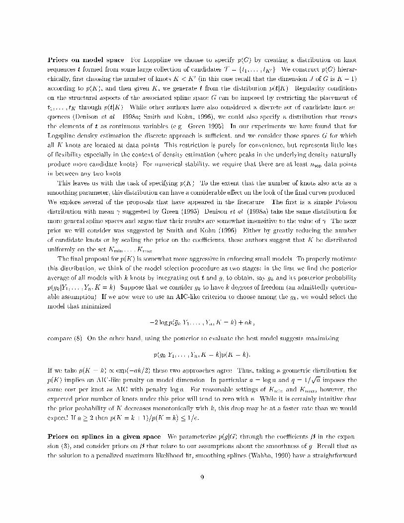
normal slight bimodal sharp peak

Fig. 1. Densities used in the simulation study.knots can be positioned at any data point that is at least nsep data points removed from one of the currentknots. Subject to this constraint, knot addition follows a simple two step procedure. First, we select oneof the intervals (L; t1); (t1; t2); : : : ; (tK ; U) uniformly at random (where the tk are the current breakpoints).Within this interval, the candidate knot is then selected uniformly at random from one of the allowable datapoints. When moving a knot, we either propose a large move (in which a knot is �rst deleted, and thenadded using the addition scheme just described) or a small move (in which the knot is only moved withinthe interval between its two neighbors). Each of these two proposals have probability (1� dJ � bJ)=2.After each reversible jump step, we update the coe�cients �. To do this, we use the fact that for a givenset of knots, we have a parametric model, and that the posterior distribution of � given G, K and the data isthus approximately multivariate normal with covariance matrix � = (�A+H)�1, and mean �Hb�, where b�is the maximum likelihood estimate of � in G, and H is the Hessian of the log-likelihood function at b�. Anobservation from this distribution is used as a proposal in a Metropolis step. Because we are using (partiallyimproper) smoothing priors, the acceptance ratio for this proposal is formally undetermined (recall that theprior covariance matrices are degenerate). We solve this problem by \canceling" the zero eigenvalue in thenumerator and the denominator (see also Besag and Higdon, 1999).2.2 A simulation studyTo compare the performance of the various possible implementations of Logspline density model selectionprocedures, we carried out a simulation study. We generated data from three densities:normal the standard normal density;slight bimodal f(y) = 0:5�fZ(y; 1:25; 1)+0:5�fZ(y;�1:25; 1:1), where fZ(y;�; �) is the normal densitywith mean � and standard deviation �;sharp peak f(y) = 0:8 � g(y) + 0:2 � f)Z(y; 2; :07), where g(Y ) is the density of the lognormal randomvariable Y = exp(Z=2) and Z has a standard normal distribution.These three densities are displayed in Figure 1. From each we generated 100 independent samples of sizen = 50, 200, 1000, and 10000. We applied a variety of Logspline methods, see Table 1. For all the Bayesian11

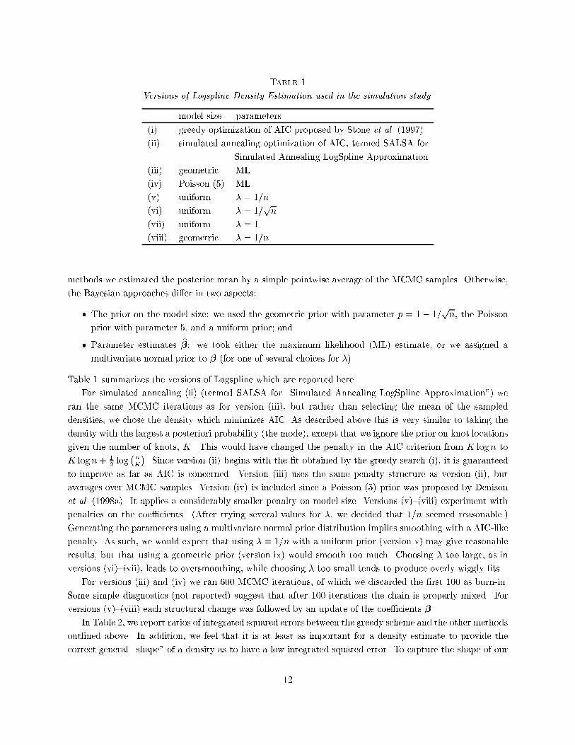
Table 1Versions of Logspline Density Estimation used in the simulation study.model size parameters(i) greedy optimization of AIC proposed by Stone et al. (1997)(ii) simulated annealing optimization of AIC, termed SALSA forSimulated Annealing LogSpline Approximation(iii) geometric ML(iv) Poisson (5) ML(v) uniform � = 1=n(vi) uniform � = 1=pn(vii) uniform � = 1(viii) geometric � = 1=nmethods we estimated the posterior mean by a simple pointwise average of the MCMC samples. Otherwise,the Bayesian approaches di�er in two aspects:� The prior on the model size: we used the geometric prior with parameter p = 1� 1=pn, the Poissonprior with parameter 5, and a uniform prior; and� Parameter estimates b�: we took either the maximum likelihood (ML) estimate, or we assigned amultivariate normal prior to � (for one of several choices for �).Table 1 summarizes the versions of Logspline which are reported here.For simulated annealing (ii) (termed SALSA for \Simulated Annealing LogSpline Approximation") weran the same MCMC iterations as for version (iii), but rather than selecting the mean of the sampleddensities, we chose the density which minimizes AIC. As described above this is very similar to taking thedensity with the largest a posteriori probability (the mode), except that we ignore the prior on knot locationsgiven the number of knots, K. This would have changed the penalty in the AIC criterion from K logn toK logn+ 12 log �nK�. Since version (ii) begins with the �t obtained by the greedy search (i), it is guaranteedto improve as far as AIC is concerned. Version (iii) uses the same penalty structure as version (ii), butaverages over MCMC samples. Version (iv) is included since a Poisson (5) prior was proposed by Denisonet al. (1998a). It applies a considerably smaller penalty on model size. Versions (v){(viii) experiment withpenalties on the coe�cients. (After trying several values for �, we decided that 1=n seemed reasonable.)Generating the parameters using a multivariate normal prior distribution implies smoothing with a AIC-likepenalty. As such, we would expect that using � = 1=n with a uniform prior (version v) may give reasonableresults, but that using a geometric prior (version ix) would smooth too much. Choosing � too large, as inversions (vi){(vii), leads to oversmoothing, while choosing � too small tends to produce overly wiggly �ts.For versions (iii) and (iv) we ran 600 MCMC iterations, of which we discarded the �rst 100 as burn-in.Some simple diagnostics (not reported) suggest that after 100 iterations the chain is properly mixed. Forversions (v){(viii) each structural change was followed by an update of the coe�cients �.In Table 2, we report ratios of integrated squared errors between the greedy scheme and the other methodsoutlined above. In addition, we feel that it is at least as important for a density estimate to provide thecorrect general \shape" of a density as to have a low integrated squared error. To capture the shape of our12

Table 2Mean Integrated Squared Error (MISE) for the simulation study.version (i) (ii) (iii) (iv) (v) (vi) (vii) (viii)distribution n MISE ratio of MISE over MISE of the greedy version (i)normal 50 0.02790 0.73 1.52 1.84 0.66 0.40 0.26 0.67normal 200 0.01069 0.49 0.60 1.23 0.79 0.50 0.24 0.66normal 1000 0.00209 0.59 0.58 1.33 0.87 0.90 0.42 0.73normal 10000 0.00020 0.33 0.49 1.45 1.35 1.10 0.80 0.87slight bimodal 50 0.02502 0.88 1.09 1.34 0.48 0.36 0.36 0.50slight bimodal 200 0.00770 0.80 0.61 1.14 0.70 0.38 0.46 0.61slight bimodal 1000 0.00164 0.57 0.60 1.13 0.89 0.66 0.40 0.77slight bimodal 10000 0.00020 0.77 0.61 0.88 0.71 0.82 0.51 0.84sharp peak 50 0.15226 0.97 0.78 0.81 0.68 0.90 1.12 0.72sharp peak 200 0.03704 0.89 0.75 0.94 0.93 2.02 3.62 1.13sharp peak 1000 0.00973 0.81 0.67 0.81 0.67 2.01 8.90 0.74sharp peak 10000 0.00150 0.72 0.57 0.57 0.64 0.58 21.43 0.76average 1.00 0.71 0.74 1.12 0.78 0.89 3.21 0.75estimates, we counted the number of times that a scheme produced densities having too few, too many andthe correct number of modes. These results are summarized in Tables 3 and 4. Table 5 calculates the \total"lines of Tables 3 and 4. Note that for simulations of a normal distribution it is not possible for an estimateto have too few modes.From Table 2 we note that most methods show a moderate overall improvement over the greedy versionof Logspline, except for (vii). This scheme oversmoothes the data, so that the details (like the mode in thesharp peaked distribution) are frequently missed. We note that version (ii), choosing the mode of a Bayesianapproach, is the only version that outperforms the greedy version for all 12 simulation set-ups. Otherwise,the di�erence between versions (ii), (iii), and (viii) seems to be minimal. In particular, if we had chosenanother set of results than those for (i) to normalize by, the order of the average MISE for these four methodswas often changed.From Table 3 we note that version (vii), and to a lesser extent (ii) and (vi), have trouble with the slightbimodal density, preferring a model with just one peak. Versions (vi) and (vii) �nd too few modes, leadingus to conclude that � should be chosen smaller than 1=pn when using a uniform prior on model size. Onthe other hand, the Poisson prior leads to models exhibiting too many peaks, as do versions (iii) and (v).Overall, it appears that the greedy, stepwise search is not too bad. It is several orders of magnitude fasterthan any of the other methods. The greedy approach, as well as SALSA have the advantage that the �nalmodel is again a Logspline density, which can be stored for later use. For the other methods, we must recordthe posterior mean at a number points. This has the potential of complicating later uses of our estimate.Among the Bayesian versions that employ ML estimates, version (iii) seems to perform best overall, whileamong those that put a prior on the coe�cient vector, versions (v) and (viii) (both of which set � = 1=n)are best. It is somewhat surprising that version (viii) performs so well, since it e�ectively imposes twice theAIC penalty on model size: one coming from the geometric prior, and one from the normal prior on the13

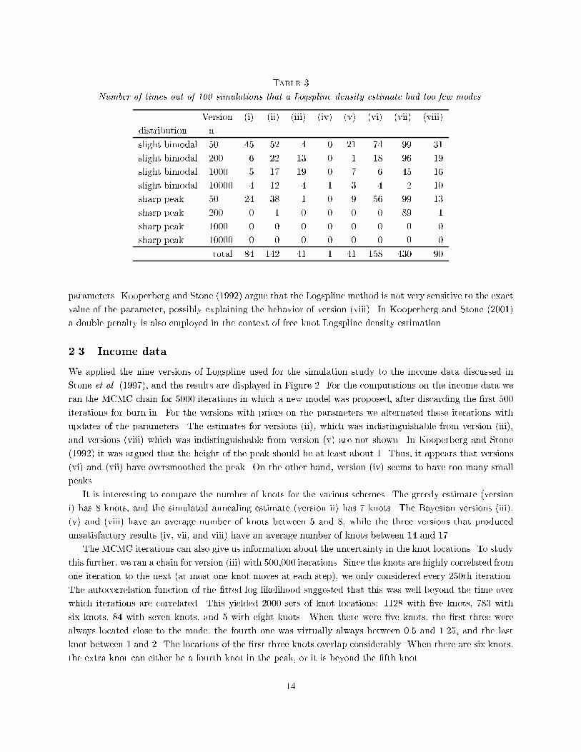
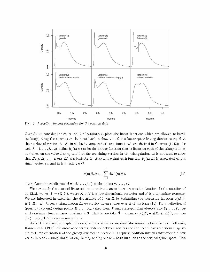
Table 3Number of times out of 100 simulations that a Logspline density estimate had too few modes.Version (i) (ii) (iii) (iv) (v) (vi) (vii) (viii)distribution nslight bimodal 50 45 52 4 0 21 74 99 31slight bimodal 200 6 22 13 0 1 18 96 19slight bimodal 1000 5 17 19 0 7 6 45 16slight bimodal 10000 4 12 4 1 3 4 2 10sharp peak 50 24 38 1 0 9 56 99 13sharp peak 200 0 1 0 0 0 0 89 1sharp peak 1000 0 0 0 0 0 0 0 0sharp peak 10000 0 0 0 0 0 0 0 0total 84 142 41 1 41 158 430 90parameters. Kooperberg and Stone (1992) argue that the Logspline method is not very sensitive to the exactvalue of the parameter, possibly explaining the behavior of version (viii). In Kooperberg and Stone (2001)a double penalty is also employed in the context of free knot Logspline density estimation.2.3 Income data.We applied the nine versions of Logspline used for the simulation study to the income data discussed inStone et al. (1997), and the results are displayed in Figure 2. For the computations on the income data weran the MCMC chain for 5000 iterations in which a new model was proposed, after discarding the �rst 500iterations for burn-in. For the versions with priors on the parameters we alternated these iterations withupdates of the parameters. The estimates for versions (ii), which was indistinguishable from version (iii),and versions (viii) which was indistinguishable from version (v) are not shown. In Kooperberg and Stone(1992) it was argued that the height of the peak should be at least about 1. Thus, it appears that versions(vi) and (vii) have oversmoothed the peak. On the other hand, version (iv) seems to have too many smallpeaks.It is interesting to compare the number of knots for the various schemes. The greedy estimate (versioni) has 8 knots, and the simulated annealing estimate (version ii) has 7 knots. The Bayesian versions (iii),(v) and (viii) have an average number of knots between 5 and 8, while the three versions that producedunsatisfactory results (iv, vii, and viii) have an average number of knots between 14 and 17.The MCMC iterations can also give us information about the uncertainty in the knot locations. To studythis further, we ran a chain for version (iii) with 500,000 iterations. Since the knots are highly correlated fromone iteration to the next (at most one knot moves at each step), we only considered every 250th iteration.The autocorrelation function of the �tted log-likelihood suggested that this was well beyond the time overwhich iterations are correlated. This yielded 2000 sets of knot locations: 1128 with �ve knots, 783 withsix knots, 84 with seven knots, and 5 with eight knots. When there were �ve knots, the �rst three werealways located close to the mode, the fourth one was virtually always between 0.5 and 1.25, and the lastknot between 1 and 2. The locations of the �rst three knots overlap considerably. When there are six knots,the extra knot can either be a fourth knot in the peak, or it is beyond the �fth knot.14

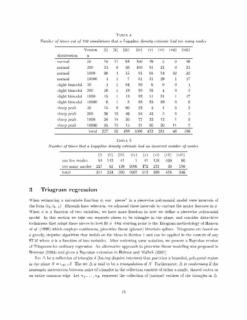
Table 4Number of times out of 100 simulations that a Logspline density estimate had too many modes.Version (i) (ii) (iii) (iv) (v) (vi) (vii) (viii)distribution nnormal 50 18 11 94 100 49 5 0 28normal 200 34 9 38 100 81 21 0 24normal 1000 26 4 15 91 68 54 32 32normal 10000 4 1 7 61 31 29 1 17slight bimodal 50 4 1 84 99 6 0 0 4slight bimodal 200 16 1 19 99 55 4 0 5slight bimodal 1000 15 1 13 93 51 31 1 17slight bimodal 10000 6 1 8 68 33 39 0 6sharp peak 50 15 8 90 93 3 1 0 2sharp peak 200 36 19 46 94 43 5 0 5sharp peak 1000 28 14 30 77 32 12 1 9sharp peak 10000 25 12 15 31 20 30 11 7total 227 82 459 1006 472 231 46 156Table 5Number of times that a Logspline density estimate had an incorrect number of modes.(i) (ii) (iii) (iv) (v) (vi) (vii) (viii)too few modes 84 142 41 1 41 158 430 90too many modes 227 82 459 1006 472 231 46 156total 311 224 500 1007 513 389 476 2463. Triogram regressionWhen estimating a univariate function �, our \pieces" in a piecewise polynomial model were intervals ofthe form (tk; tk+1). Through knot selection, we adjusted these intervals to capture the major features in �.When � is a function of two variables, we have more freedom in how we de�ne a piecewise polynomialmodel. In this section we take our separate pieces to be triangles in the plane, and consider data-drivetechniques that adapt these pieces to best �t �. Our starting point is the Triogram methodology of Hansenet al. (1998) which employs continuous, piecewise linear (planar) bivariate splines. Triograms are based ona greedy, stepwise algorithm that builds on the ideas in Section 1 and can be applied in the context of anyELM where � is a function of two variables. After reviewing some notation, we present a Bayesian versionof Triograms for ordinary regression. An alternative approach to piecewise linear modeling was proposed inBrieman (1993) and given a Bayesian extension in Holmes and Mallick (2001).Let 4 be a collection of triangles � (having disjoint interiors) that partition a bounded, polygonal regionin the plane X = [�24�. The set 4 is said to be a triangulation of X . Furthermore, 4 is conforming if thenonempty intersection between pairs of triangles in the collection consists of either a single, shared vertex oran entire common edge. Let v1; : : : ;vK represent the collection of (unique) vertices of the triangles in 4.15

0.5 1.5 2.5 0.5 1.5 2.5 0.5 1.5 2.5

0.0

0.5

1.0

0.0

0.5

1.0

version (i)greedy

version(iii)geometric

version(iv)Poisson(5)

version(v)uniform lambda=1/n

version(vi)uniform lambda=1/sqrt(n)

version(vii)uniform lambda=1

Income Income Income

Den

sity

Den

sity

Fig. 2. Logspline density estimates for the income data.Over X , we consider the collection G of continuous, piecewise linear functions which are allowed to break(or hinge) along the edges in 4. It is not hard to show that G is a linear space having dimension equal tothe number of vertices K. A simple basis composed of \tent functions" was derived in Courant (1943): Foreach j = 1; : : : ;K, we de�ne Bj(x;4) to be the unique function that is linear on each of the triangles in 4and takes on the value 1 at vj and 0 at the remaining vertices in the triangulation. It is not hard to showthat B1(x;4); : : : ; BK(x;4) is a basis for G. Also notice that each function Bj(x;4) is associated with asingle vertex vj , and in fact each g 2 Gg(x;�;4) = JXi=1 �iBi(x;4); (11)interpolates the coe�cients � = (�1; : : : ; �K) at the points v1; : : : ;vK .We now apply the space of linear splines to estimate an unknown regression function. In the notation ofan ELM, we let W = (X; Y ), where X 2 X is a two-dimensional predictor and Y is a univariate response.We are interested in exploring the dependence of Y on X by estimating the regression function �(x) =E(Y jX = x). Given a triangulation 4, we employ linear splines over 4 of the form (11). For a collection of(possibly random) design points X1; : : : ;Xn taken from X and corresponding observations Y1; : : : ; Yn, weapply ordinary least squares to estimate �. That is, we take b� = argmax�Pi[Yi � g(Xi;�;4)]2, and usebg(x) = g(x; b�;4) as an estimate for �.As with the univariate spline models, we now consider stepwise alterations to the space G. FollowingHansen et al. (1998), the one-to-one correspondence between vertices and the \tent" basis functions suggestsa direct implementation of the greedy schemes in Section 1. Stepwise addition involves introducing a newvertex into an existing triangulation, thereby adding one new basis function to the original spline space. This16

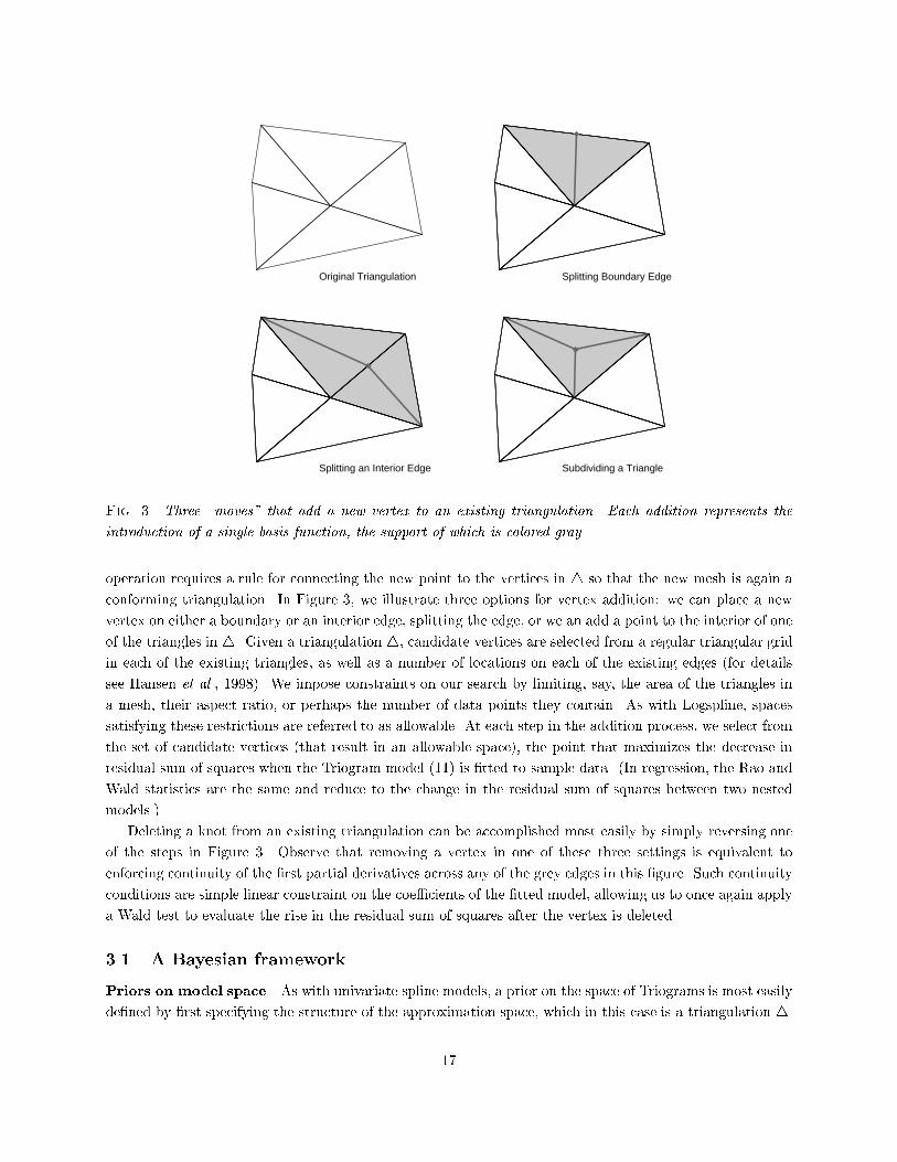
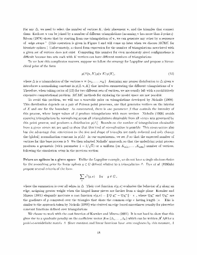
Original Triangulation Splitting Boundary Edge

Splitting an Interior Edge Subdividing a TriangleFig. 3. Three \moves" that add a new vertex to an existing triangulation. Each addition represents theintroduction of a single basis function, the support of which is colored gray.operation requires a rule for connecting the new point to the vertices in 4 so that the new mesh is again aconforming triangulation. In Figure 3, we illustrate three options for vertex addition: we can place a newvertex on either a boundary or an interior edge, splitting the edge, or we an add a point to the interior of oneof the triangles in 4. Given a triangulation 4, candidate vertices are selected from a regular triangular gridin each of the existing triangles, as well as a number of locations on each of the existing edges (for detailssee Hansen et al., 1998). We impose constraints on our search by limiting, say, the area of the triangles ina mesh, their aspect ratio, or perhaps the number of data points they contain. As with Logspline, spacessatisfying these restrictions are referred to as allowable. At each step in the addition process, we select fromthe set of candidate vertices (that result in an allowable space), the point that maximizes the decrease inresidual sum of squares when the Triogram model (11) is �tted to sample data. (In regression, the Rao andWald statistics are the same and reduce to the change in the residual sum of squares between two nestedmodels.)Deleting a knot from an existing triangulation can be accomplished most easily by simply reversing oneof the steps in Figure 3. Observe that removing a vertex in one of these three settings is equivalent toenforcing continuity of the �rst partial derivatives across any of the grey edges in this �gure. Such continuityconditions are simple linear constraint on the coe�cients of the �tted model, allowing us to once again applya Wald test to evaluate the rise in the residual sum of squares after the vertex is deleted.3.1 A Bayesian frameworkPriors on model space As with univariate spline models, a prior on the space of Triograms is most easilyde�ned by �rst specifying the structure of the approximation space, which in this case is a triangulation 4.17

For any 4, we need to select the number of vertices K, their placement v, and the triangles that connectthem. Each set v can be joined by a number of di�erent triangulations (assuming v has more than 3 points).Sibson (1978) shows that by starting from one triangulation of v, we can generate any other by a sequenceof \edge swaps." (This operation is given in Figure 4 and will come up later when we discuss MCMC forbivariate splines.) Unfortunately, a closed-form expression for the number of triangulations associated witha given set of vertices does not exist. Computing this number for even moderately sized con�gurations isdi�cult because two sets each with K vertices can have di�erent numbers of triangulations.To see how this complicates matters, suppose we follow the strategy for Logspline and propose a hierar-chical prior of the form p(4jv;K) p(vjK) p(K); (12)where 4 is a triangulation of the vertices v = fv1; : : : ;vKg. Assigning any proper distribution to 4 given vintroduces a normalizing constant in p(4jv;K) that involves enumerating the di�erent triangulations of v.Therefore, when taking ratios of (12) for two di�erent sets of vertices, we are usually left with a prohibitivelyexpensive computational problem. MCMC methods for exploring the model space are not possible.To avoid this problem, we will use a tractable prior on triangulations developed by Nicholls (1998).This distribution depends on a pair of Poisson point processes, one that generates vertices on the interiorof X and one for the boundary. As constructed, there is one parameter � that controls the intensity ofthis process, where larger values of � produce triangulations with more vertices. Nicholls (1998) avoidscounting triangulations by normalizing across all triangulations obtainable from all vertex sets generated bythis point process, and produces a distribution p(4). Bounds on the number of triangulations obtainablefrom a given vertex set are used to show that this kind of normalization is possible. This construction alsohas the advantage that restrictions on the size and shape of triangles are easily enforced and only changethe (global) normalization constant in p(4). In our experiments, we set � so that the expected number ofvertices for this base process is 5. We then adapted Nicholls' approach, so that the underlying point processproduces a geometric (with parameter 1 � 1=pn) or a uniform (on Kmin; : : : ;Kmax) number of vertices,following the simulation setup in the previous section.Priors on splines in a given space Unlike the Logspline example, we do not have a single obvious choicefor the smoothing prior for linear splines g 2 G de�ned relative to a triangulation 4. Dyn et al. (1990ab)propose several criteria of the form Xe s2(g; e) for g 2 G ;where the summation is over all edges in 4. Their cost function s(g; e) evaluates the behavior of g along anedge, assigning greater weight when the hinged linear pieces are farther from a single plane. Koenker andMizera (2001) elegantly motivate a cost function s(g; e) = k 5 g+e �5g�e k � kek, where 5g+e and 5g�e arethe gradients of g computed over the triangles that share the common edge e having length kek. This issimilar to the approach taken by Nicholls (1998) who derived an edge-based smoothness penalty for piecewiseconstant functions de�ned over triangulations.We choose to work with the cost function of Koenker and Mizera (2001). It is not hard to show that thisgives rise to a quadratic penalty on the coe�cient vector � = (�1; : : : ; �K) which can be written �tA� for apositive-semide�nite matrix A. Since constant and linear functions have zero roughness by this measure, A18

Original Triangulation Swapping a Diagonal Moving a VertexFig. 4. Additional structural moves for the reversible jump MCMC scheme. Note that these two proposalsresult in a non-nested sequence of spaces.has two zero eigenvalues. As was done for Logspline, we use A to generate a partially improper normal prioron � (with prior variance ��2, where �2 is the error variance). Following Denison et al. (1998a), we assigna proper, inverse-gamma distribution to �, and experiment with various �xed choices for � that depend onsample size.Markov chain Monte Carlo Our approach to MCMC for Triograms is similar to that with Logsplineexcept that we need to augment our set of structural changes to 4 to include more moves than simple vertexaddition and deletion. In Figure 4, we present two additional moves that maintain the dimension of thespace G but change its structure. The middle panel illustrates swapping an edge, an operation that we havealready noted is capable of generating all triangulations of a given vertex set v. Quak and Schumaker (1991)use random swaps of this kind to come up with a good triangulation for a �xed set of vertices. In in the�nal panel of Figure 4, we demonstrate moving a vertex inside the union of triangles that contain it. Thesechanges to 4 are non-nested in the sense that they produce spline spaces that do not di�er by the presenceor absence of a single basis function. For Triograms, the notion of an allowable space can appear through sizeor aspect ratio restrictions on the triangulations, and serves to limit the region in which we can place newvertices or to which we can move existing vertices. For example, given a triangle, the set into which we caninsert a new vertex and still maintain a minimum area condition is a subtriangle, easily computable in termsof barycentric coordinates (see Hansen et al. 1998). As with Logspline, we alternate between these structuralmoves and updating the model parameters. Because we are working with regression, we can integrate out� and only have to update �2 at each pass. This approach allows us to focus on structural changes as wasdone by Smith and Kohn (1996) for univariate regression.3.2 SimulationsIn Figure 5, we present a series of three �ts to a simulated surface plotted in the upper lefthand corner. Adata set consisting of 100 observations was generated by �rst sampling 100 design points uniformly in theunit square. The actual surface is described by the functionf(x) = 40 expf8[(x1 � 0:5)2 + (x2 � 0:5)2]gexpf8[(x1 � 0:2)2 + (x2 � 0:7)2]g+ expf8[(x1 � 0:7)2 + (x2 � 0:2)2]g ;19

0.2

0.40.6

0.8

X

0.20.4

0.60.8

Y

True surface

0.2

0.40.6

0.8

X

0.20.4

0.60.8

Y

Model averaging, smoothing prior

0

0.2

0.40.6

0.8

1

X

00.2

0.40.6

0.81

Y

Greedy fit

0

0.2

0.40.6

0.8

1

X

00.2

0.40.6

0.81

Y

Simulated annealing

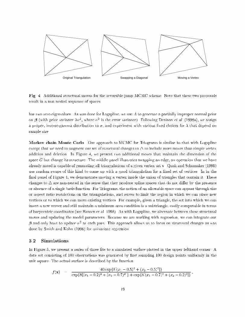
Fig. 5. In the top row we have the true surface (left) and the �t resulting from model averaging (right). Inthe bottom row we have two isolated �ts, each a \minimal" BIC model, the leftmost coming from a greedysearch, and the rightmost produced by simulated annealing (the triangulations appear at the top of eachpanel).to which we add standard Gaussian errors. This function �rst appeared in Gu et al. (1990), and it willbe hereafter referred to as simply GBCW. The signal-to-noise ratio in this setup is about 3. In the lowerlefthand panel in Figure 5, we present the result of applying the greedy, Triogram algorithm. As is typical,the procedure has found a fairly regular, low-dimensional mesh describing the surface (the MISE is 0.31).For the �t plotted in the lower righthand panel, we employed a simulated annealing scheme similar to thatdescribed for Logspline. The geometric prior for 4 is used to guide the sampler through triangulations, andin each corresponding spline space G we consider bg, the MLE (or in this case the ordinary least squares�t). In this way, the objective function matches that of the greedy search, the generalized AIC criterion(8). The scheme alternates between (randomly selected) structural changes (edge swaps and vertex moves,additions and deletions) and updating the estimate b�2 of the noise variance. After 6,000 iterations, thesampler has managed to �nd a less regular, and marginally poorer-�tting model (the MISE is 0.32). In thecontext of triangulations, the greedy search is subject to a certain regularity that prevents con�gurationslike the one in Figure 5. We can recapture this in the MCMC simulations either by placing restrictions onthe triangulations in each mesh (say, imposing a smallest allowable size or aspect ratio) or by increasing thepenalty on dimension, speci�ed through our geometric prior.In the last panel, we present the result of model averaging using a uniform prior on model size and a20

Table 6.Versions of Triogram used in the simulation study.model size parameters(i) greedy optimization of BIC(ii) simulated annealing optimization of BIC(iii) Poisson (5) ML(iv) geometric ML(v) uniform � = 1=nsmoothing prior on the coe�cients (� = 1=n). The sampler is run for a total of 6,000 iterations, of which1,000 are discarded as burn-in. We then estimate the posterior mode as a pointwise average of the sampledsurfaces. The �nal �t is smoother in part because we are combining many piecewise-planar surfaces. Westill see sharp e�ects, however, where features like the central ridge are present. The model in the lowerrighthand panel is not unlike the surfaces visited by this chain. As spaces G are generated, the central spine(along the line y = x) of this surface is always present. The same is true for the hinged portions of thesurface along the lines x = 0 and y = 0. With these caveats in mind, the MISE of the averaged surface isabout half of the other two estimates (0.15). Table 7.Mean Integrated Squared Error (MISE) for two smooth test functions.version (i) (ii) (iii) (iv) (v)distribution n MISE ratio of MISE over (i)GBCW (high snr) 100 0.31 1.35 0.85 0.78 0.77GBCW (high snr) 500 0.10 1.0 0.64 0.76 0.80GBCW (high snr) 1000 0.08 0.91 0.82 0.94 0.79Exp (low snr) 100 0.15 0.90 0.52 0.51 0.49Exp (low snr) 500 0.04 0.85 0.46 0.50 0.47Exp (low snr) 1000 0.03 0.51 0.32 0.40 0.46We repeated these simulations for several sample sizes, taking n = 100, 500 and 1000 (100 repetitions foreach value of n). In Table 6, we present several variations in the prior speci�cation and search procedure.In addition to GBCW, we also borrow a test function from Breiman (1991), which we will refer to asExp. Here, points X = (X1; X2) are selected uniformly from the square [�1; 1]2. The response is given byexp(x1 sin(�x2)) to which normal noise is added (� = 0:5). The signal-to-noise ratio in this setup is muchlower, 0.9. The results are presented in Table 7. It seems reasonably clear that the simulated annealingapproach can go very wrong, especially when the sample size is small. Again, this argues for the use ofgreater constraints in terms of allowable spaces when n is moderate. It seems that model averaging withthe smoothing prior (� = 1=n) and the Poisson prior of Denison et al. (1998a) perform the best. A closerexamination of the �tted surfaces reveals the same kinds of secondary structure as we saw in Figure 5. Tobe sure, smoother basis functions would eliminate this behavior. It is not clear at present, however, if adi�erent smoothing prior on the coe�cients might serve to \unkink" these �ts.21

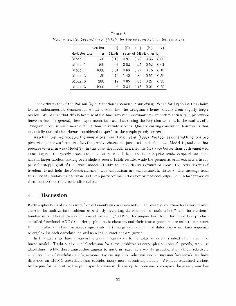
Table 8Mean Integrated Squared Error (MISE) for two piecewise-planar test functionsversion (i) (ii) (iii) (iv) (v)distribution n MISE ratio of MISE over (i)Model 1 50 0.16 0.97 0.70 0.35 0.80Model 1 200 0.04 0.82 0.95 0.52 0.62Model 1 1000 0.01 0.63 0.72 0.76 0.40Model 3 50 0.70 1.40 0.86 0.51 0.50Model 3 200 0.17 0.85 0.63 0.27 0.30Model 3 1000 0.03 0.34 0.45 0.21 0.20The performance of the Poisson (5) distribution is somewhat surprising. While for Logspline this choiceled to undersmoothed densities, it would appear that the Triogram scheme bene�ts from slightly largermodels. We believe that this is because of the bias involved in estimating a smooth function by a piecewise-linear surface. In general, these experiments indicate that tuning the Bayesian schemes in the context of aTriogram model is much more di�cult than univariate set-ups. One comforting conclusion, however, is thatessentially each of the schemes considered outperform the simple greedy search.As a �nal test, we repeated the simulations from Hansen et al. (1998). We took as our trial functions twopiecewise planar surfaces, one that the greedy scheme can jump to in a single move (Model 1), and one thatrequires several moves (Model 3). In this case, the model averaged �ts (iv) were better than both simulatedannealing and the greedy procedure. The estimate built from the Poisson prior tends to spend too muchtime in larger models, leading to its slightly poorer MISE results, while the geometric prior extracts a heavyprice for stepping o� of the \true" model. (Unlike the smooth cases examined above, the extra degrees offreedom do not help the Poisson scheme.) The simulations are summarized in Table 8. One message fromthis suite of simulations, therefore, is that a posterior mean does not over-smooth edges, and in fact preservesthem better than the greedy alternatives.4. DiscussionEarly applications of splines were focused mainly on curve estimation. In recent years, these tools have provede�ective for multivariate problems as well. By extending the concepts of \main e�ects" and \interactions"familiar in traditional d�way analysis of variance (ANOVA), techniques have been developed that produceso-called functional ANOVA's. Here, spline basis elements and their tensor products are used to constructthe main e�ects and interactions, respectively. In these problems, one must determine which knot sequenceto employ for each covariate, as well as what interactions are present.In this paper we have discussed a general framework for adaptation in the context of an extendedlinear model. Traditionally, model-selection for these problems is accomplished through greedy, stepwisealgorithms. While these approaches appear to perform reasonably well in practice, they visit a relativelysmall number of candidate con�gurations. By casting knot selection into a Bayesian framework, we havediscussed an MCMC algorithm that samples many more promising models. We have examined varioustechniques for calibrating the prior speci�cations in this setup to more easily compare the greedy searches22

and the MCMC schemes. An e�ective penalty on model size can be imposed either explicitly (through a priordistribution on dimension), or through the smoothness prior assigned to the coe�cient vector. In general,we have demonstrated a gain in �nal mean squared error when appealing to the more elaborate samplingschemes.We have also gone to great lengths to map out connections between this Bayesian method and otherapproaches to the knot placement problem. For example, a geometric prior distribution on model size, hasa natural link to (stepwise) model selection with BIC, while we can choose a multivariate normal prior onthe coe�cients to connect us with the penalized likelihood methods employed in classical smoothing splines.In addition, the Bayesian formalism allows us to account for the uncertainty in both the structural aspectsof our estimates (knot con�gurations and triangulations) as well as the coe�cients in any given expansion.Model averaging in this context seems to provide improvement over simply selecting a single \optimal" modelin terms of say BIC. The disadvantage of this approach is that we do not end up with a model based on oneset of knots (or one triangulation).While running our experiments, we quickly reached the conclusion that the priors play an important role:an inappropriate prior can easily lead to results that are much worse than the greedy algorithms. However, inour experiments we found out that when the priors are in the right ballpark, Bayesian procedures do performsomewhat better than greedy schemes in a mean squared error sense. This improvement in performanceis larger for a relatively \unstable" procedures such as Triogram, while the improvement for a \stable"procedure such as Logspline is smaller.For the Triogram methodology there is an additional e�ect of model averaging: the average of manypiecewise planar surfaces will give the impression of being smoother. Whether this is an advantage or notprobably depends on the individual user and her/his application: when we gave seminars about the originalTriogram paper, there were people who saw the piecewise planar approach as a major strength and as amajor weakness of the methodology.AcknowledgementsCharles Kooperberg was supported in part by National Institutes of Health grant R29 CA 74841. Theauthors wish to thank Merlise Clyde, David Denison, Ed George, Peter Green, Robert Kohn and Bin Yu formany helpful discussions.ReferencesAkaike, H. (1974) A new look at the statistical model identi�cation. IEEE Trans. AC, 19 716{723.Besag, J. and Higdon, D. (1999) Bayesian inference for agricultural �eld experiments (with discussion). J.R. Statist. Soc. B, 61, 691{746.Breiman, L. (1991) The �-method for estimating multivariate functions from noisy data. Technometrics,33, 125{143.Breiman, L. (1993) Hinging hyperplanes for regression, classi�cation and function approximation, IEEETrans. Info. Theory, 3(3), 999{1013.Breiman, L., Friedman, J. H., Olshen, R. A. and Stone, C. J. (1984) Classi�cation and Regression Trees.Paci�c Grove, California: Wadsworth. 23

Courant, R. (1943) Variational methods for the solution of problems of equilibrium and vibrations. Bull.Am. Math. Soc., 49, 1{23.de Boor, C. (1978) A Practical Guide to Splines. New York: Springer.Denison, D. G. T., Mallick, B. K. and Smith, A. F. M. (1998a) Automatic Bayesian curve �tting. J. R.Statist. Soc. B, 60, 333{350.Denison, D. G. T., Mallick, B. K. and Smith, A. F. M. (1998b) A Bayesian CART algorithm. Biometrika,85, 363{377.Dyn, N., Levin, D. and Rippa, S. (1990a) Data dependent triangulations for piecewise linear interpolation.IMA J. Num. Anal., 10, 137{154.Dyn, N., Levin, D. and Rippa, S. (1990b) Algorithms for the construction of data dependent triangulations.Alg. Approx. (eds. J. C. Mason and M. G. Cox, M. G), vol II, pp. 185{192. New York: Chapman andHall.Friedman, J. H. (1991) Multivariate adaptive regression splines (with discussion). Ann Statist, 19, 1{141.Friedman, J. H. and Silverman, B. W. (1989) Flexible parsimonious smoothing and additive modeling (withdiscussion). Technometrics, 31, 3{39.Green, P. J. (1995) Reversible jump Markov chain Monte Carlo computation and Bayesian model determi-nation. Biometrika, 82, 711{732.Green, P. J. and Silverman, B. W. (1994) Nonparametric Regression and Generalized Linear Models. Lon-don: Chapman and Hall.Gu, C., Bates, D. M., Chen, Z. and Wahba, G. (1990) The computation of GCV function through House-holder tridiagonlization with application to the �tting of interaction spline models. SIAM J. Mat.Anal., 10, 457{480.Halpern, E. F. (1973) Bayesian spline regression when the number of knots is unknown. J. R. Statist. Soc.B, 35, 347{360.Hansen, M. (1994) Extended Linear Models, Multivariate Splines and ANOVA. Ph. D. Dissertation. Berke-ley: University of California.Hansen, M., Kooperberg, C. and Sardy, S. (1998) Triogram Models. J. Am. Statist. Assoc., 93, 101{119.Holmes, C.C. and Mallick, B.K. (2001) Bayesian regression with multivariate linear splines, J. Roy. Statist.Soc. Series B., 63, 3{18.Huang, J. Z. (1998) Projection estimation in multiple regression with application to functional ANOVAmodels. Ann. Statist., 26, 242{272.Huang, J. Z. (2001) Concave extended linear modeling: a theoretical synthesis. Statistica Sinica, 11,173{197.Jupp, D. L. B. (1978). \Approximation to Data by Splines with Free Knots," SIAM J. Num. Anal., 15,328{343.Koenker, R. and Mizera, I. (2001) Penalized Triograms: Total variation regularization for bivariate smooth-ing, Technical Report.Kooperberg, C., Bose, S. and Stone, C. J. (1997) Polychotomous Regression. J. Am. Statist. Assoc., 92,117{127. 24

Kooperberg, C., and Stone, C. J. (1991) Logspline density estimation. Comp. Statist. Data Anal., 12,327{347.Kooperberg, C., and Stone, C. J. (1992) Logspline density estimation for censored data. J. Comp. Graph.Statis., 1, 301{328.Kooperberg, C., and Stone, C. J. (2001) Logspline density with free knot splines. Manuscript.Lindstrom, M (1999) Penalized estimation of free-knot splines. J. Comp. Graph. Statis., 8, 333{352.Nicholls, G. (1998) Bayesian image analysis with Markov chain Monte Carlo and colored continuum trian-gulation models. J. R. Statist. Soc. B, in press.Quak, E. and Schumaker, L. L. (1991) Least squares �tting by linear splines on data dependent triangula-tions. In Curves and Surfaces (eds. P.J. Laurent, A. Le M�ehaut�e and L. L. Schumaker), pp. 387{390.San Diego: Academic Press.Schumaker, L. L. (1993) Spline Functions: Basic Theory. New York: Wiley.Schwarz, G. (1978) Estimating the dimension of a model. Anni. Statist., 6, 461{464.Silverman, B. W. (1985) Some aspects of the spline smoothing approach to nonparametric regression curve�tting (with discussion). J. R. Statist. Soc. B, 47, 1{52.Sibson, R. (1978) Locally equiangular triangulations. Computer Journal, 21, 243{245.Smith, M. (1996) Nonparametric Regression: A Markov chain Monte Carlo Approach. Ph. D. Dissertation.Australia: University of New South Wales.Smith, M. and Kohn, R. (1996) Nonparametric regression using Bayesian variable selection. J. Economet-rics, 75, 317{344.Smith, M. and Kohn, R. (1998) Nonparametric estimation of irregular functions with independent orautocorrelated errors. In Practical Nonparametric and Semiparametric Bayesian Statistics (eds. D.Dey, P. Mller and D. Sinha), pp. 133{150. New York: Springer-Verlag.Smith, P. L. (1982a) Curve �tting and modeling with splines using statistical variable selection techniques.Report NASA 166034. Hampton, Virginia: NASA, Langley Research Center.Smith, P.L. (1982b) Hypothesis testing in B-spline regression. Communications in Statistics, Part B{Simulation and Computation, 11, 143{157.Stone, C. J. (1985) Additive regression and other nonparametric models. Ann. Statist., 13, 689{705.Stone, C. J. (1994) The use of polynomial splines and their tensor products in multivariate function esti-mation (with discussion). Ann. Statist., 22, 118{184.Stone, C. J., Hansen M., Kooperberg, C. and Truong, Y. K. (1997) Polynomial splines and their tensorproducts in extended linear modeling (with discussion). Ann. Statist. 25, 1371{1470.Stone, C. J. and Huang, J. Z. (2001) Free knot splines in concave extended linear modeling . J. Statist.Plan. Inf., to appear.Stone, C. J. and Koo, C.-Y. (1986) Logspline density estimation. AMS Cont. Math. Ser., 59, 1{15.Wahba, G. (1990) Spline Models for Observational Data. Philadelphia: Society for Industrial and AppliedMathematics.25