on spline wavelets - sam houston state university

On Spline Wavelets

Dedicated to Professor Charles Chui on the occasionof his 65th birthday

Jianzhong Wang

Abstract. Spline wavelet is an important aspect of the constructivetheory of wavelets. This paper consists of three parts. The first partsurveys the joint work of Charles Chui and me on the constructionof spline wavelets based on the duality principle. It also includesa discussion of the computational and algorithmic aspects of splinewavelets. The second part reviews our study of asymptotically time-frequency localization of spline wavelets. The third part introducesthe application of Shannon wavelet packet in the sub-band decompo-sition in multiple-channel synchronized transmission of signals.

§1. Introduction

In this paper, I give a brief survey of my joint work with Charles Chuion spline wavelet. In the theory of wavelet analysis, an important aspectis to construct wavelet bases of a function space, say of the Hilbert spaceL2(R) ([32], [64], [65]). Recall that a (standard) wavelet basis of L2(R) isthe basis generated by the dilations and translates of a “wavelet” functionψ. More precisely, if the set of functions

{ψj,k}j,k∈Z , ψj,k = 2j/2ψ(2jx− k), (1)

forms an unconditional basis (also called a Riesz basis) of L2(R),then we call ψ a wavelet and call the system (1) a wavelet basis. Threeof most basic properties of a wavelet are its regularity, its decay speed,and the order of its vanishing moments. Therefore, a wavelets is usuallychosen to be compactly supported (or exponentially decay) and to havecertain degree of regularity so that they are “local” in both x-domain (timedomain) and ω-domain (frequency domain). Then each element in the

Conference Title 1Editors pp. 1–6.

Copyright Oc 2005 by Nashboro Press, Brentwood, TN.

ISBN 0-0-9728482-x-x

All rights of reproduction in any form reserved.

2 J.Z. Wang

wavelet basis (1) has a finite time-frequency window. Thus, wavelet basesare useful tools for “local” analysis of functions. Many books and papersalready explain the importance of wavelet bases in harmonic analysis andin various applications. (See [6], [7], [32], [49], [64], [65].)

In the earlier time in the history of wavelet analysis, people tried toconstruct a wavelet basis by finding the wavelet function ψ directly. It isMayer and Mallat who create Multiresolution Analysis (MRA) [64], [65],which provides a powerful framework for the construction of wavelet bases.

Definition 1. A multiresolution analysis of L2 is a nest of subspaces ofL2:

· · · ⊂ V−1 ⊂ V0 ⊂ V1 ⊂ · · ·that satisfies the following conditions.

(1) ∩j∈ZVj = {0},(2) ∪j∈ZVj = L2,(3) f(·) ∈ Vj if and only if f(2·) ∈ Vj+1, and(4) there exists a function φ ∈ V0 such that {φ(x − n)}n∈Z is an

unconditional basis of V0, i.e. {φ(x−n)}n∈Z is a basis of V0, and thereexist two constants A,B > 0 such that, for all (cn) ∈ l2, the followinginequality holds:

A∑

n∈Z|cn|2 ≤

∥∥∥∥∥∑

n∈Zcnφ(· − n)

∥∥∥∥∥

2

≤ B∑

n∈Z|cn|2. (2)

The function φ described in Definition 1 is called an MRA generator.Furthermore, if {φ(x − n)}n∈Z is an orthonormal basis of V0, then φ iscalled an orthonormal MRA generator. Since φ ∈ V0 is also in V1, wecan establish a two-scale equation for φ:

φ(x) = 2∑

m∈Zhmφ(2x−m), (hm)m∈Z ∈ l2, (3)

where h = (hm)m∈Z is called the mask of φ.Taking the Fourier transform of (3), we obtain

φ(ω) = H(e−iω/2)φ(ω/2), H(z) =∑

m∈Zhmzm, (4)

which represents the two-scale equation of φ in the frequency domain.Here, H(z) is the symbol of φ.

The MRA approach to wavelet basis can be described as follows. LetWj be a complement of Vj with respect to Vj+1:

Wj ⊕ Vj = Vj+1, j ∈ Z.

On Spline Wavelets 3

Then we have

L2(R) = ⊕j∈ZWj , Wj ∩Wk = {0}, j 6= k,

g ∈ Wj ⇐⇒ g(2·) ∈ Wj+1, j ∈ Z.

Let ψ ∈ W0 be such a function that {ψ(· − n)}n∈Z forms a Riesz basisof W0. Then {ψj,k}j,k∈Z forms a wavelet basis of L2(R). Since W0 ⊂ V1,

there is a sequence g ∈ l2 such that the function ψ satisfies

ψ(t) = 2∑

k∈Zgkφ(2x− k), g ∈ l2, (5)

where g = (gk) is the mask of ψ. The Fourier transform of ψ is

φ(ω) = G(e−iω/2)φ(ω/2), G(z) =∑

m∈Zgmzm,

where G(z) is the symbol of ψ. According to the analysis above, once wehave an MRA generator φ (and its mask h) to construct a wavelet basisbecomes to find the mask g of ψ.

Let us consider the decomposition of a function f ∈ L2 into the waveletseries:

f =∑

j,k∈Zdj,kψj,k (6)

orf =

∑

k∈ZcJ,kφJ,k +

∑

j≥J

∑

k∈Zdj,kψj,k. (7)

To find the coefficients (dj,k) and (cj,k) in the decompositions (6) and(7), we need the dual bases of {φj,k} and {ψj,k}, say {φj,k} and {ψj,k},respectively. The theory of the construction of wavelet bases studies themethods to find {ψj,k}, {φj,k}, and {ψj,k} from {φj,k}.

Among various wavelet bases, spline wavelet bases play an importantrole due to their beautiful structure and powerful ability in computa-tion. Spline wavelet is an important aspect of the constructive theory ofwavelets. The paper consists of three parts. The first part surveys thejoint work of Charles Chui and me on the construction of spline waveletsbased on the duality principle. It also includes a discussion of the com-putational and algorithmic aspects of spline wavelets. The second partreview our study of asymptotically time-frequency localization of splinewavelets. The third part introduces the applications of Shannon waveletpacket in the sub-band decomposition in multiple-channel synchronizedtransmission of signals. As a survey paper, the proofs of all results willnot be included. Instead, we only refer the original papers which show theproofs in details.

4 J.Z. Wang

§2. Duality Principle and Construction of Spline Wavelets

As we mentioned in the introduction, to construct a wavelet basis basedon an MRA generator φ and to compute the coefficients of the waveletseries, we need to find the relation among φ, ψ, φ, and ψ. Their relationscan be formulated to Duality principle. Charles and I established theduality principle in [16] , [17], and [18]. Its comprehensive description wasincluded in Charles’ book [6]. The book and the papers were publishedmore than ten years ago. Since then, a lot of generalizations of the dualityprinciple have been developed for multivariate wavelet bases (see [44], [45],[46], [47], [48], [53], [54], [56], [57], [58], [66], [67], [68]) , multiwavelet bases(see [14], [36], [37]), and wavelet frames (see [8], [9], [10], [12], [34], [70],[71],[72]). The references listed here are far from complete ones. Thereaders can refer the references in the papers mentioned above. However,today giving a review of the original idea of the duality principle stillmakes sense. I now introduce the principle of its original formulation in aconcise way.

Definition 2. Assume a scaling function

φ(t) = 2∑

k∈Zh(k)φ(2t− k) (8)

generates an MRA {Vj}j∈Z. If a scaling function

φ(t) = 2∑

k∈Zh(k)φ(2t− k) (9)

satisfies< φ0,n, φ0,m >= δnm, (10)

then φ is called a dual scaling function of φ.

The dual scaling function φ also generates an MRA {Vj}j∈Z, called adual MRA of {Vj}j∈Z. It is not hard to see that there is a complement ofVj with respect to Vj+1, say Wj , which satisfies

L2(R) = ⊕j∈ZWj , Wj ∩ Wk = {0}, j 6= k,

g ∈ Wj ⇐⇒ g(2·) ∈ Wj+1, j ∈ Z.

and there is a wavelet ψ ∈ W0 such that {ψjk}k∈Z forms a Riesz basis ofWj and

〈ψi,k, ψj,l〉 = δijδkl, for all i, j, k, l ∈ Z. (11)

We call ψ a dual wavelet of ψ and call {ψjk}j,k∈Z and {ψjk}j,k∈Z aredual bases of L2. There is a sequence g ∈ l2 such that the function ψsatisfies

ψ(t) = 2∑

k∈Zg(k)φ(2x− k). (12)


The relations among φ, φ, ψ, and ψ are presented in the following dualityprinciple [17], [18].

Theorem 1. Let φ and φ be the dual scaling functions with masks h =(hk) and h = (hk) respectively, and ψ and ψ be the dual wavelets definedby (5) and (12) respectively. then

2∑

k h(k)h(k − 2l) = δ0l,2

∑k g(k)g(k − 2l) = δ0l,∑k h(k)g(k − 2l) = 0,∑k h(k)g(k − 2l) = 0,

k, l ∈ Z,

which is equivalent to

H(z)H(z) + H(−z)H(−z) = 1,

G(z)G(z) + G(−z)G(−z) = 1,

G(z)H(z) + G(−z)H(−z) = 0,

G(z)H(z) + G(−z)H(−z) = 0.

z ∈ Γ, (13)

where H(z) =∑

h(k)zk, H(z) =∑

h(k)zk, G(z) =∑

g(k)zk, andG(z) =

∑g(k)zk.

By duality principle, finding φ, ψ, and ψ from φ, can be completedby finding H(z), G(z), and G(z) from H(z). Here the symbol H(z) mustsatisfy the condition such that it generates a stable scaling function φ. Wenow see how to apply the duality principle to some special cases.1. Orthonormal scaling functions and wavelets (see [63], [64]). In this

case, φ = φ and ψ = ψ. Hence, H = H and G = G. The equation(13) is reduced to

|H(z)|2 + |H(−z)|2 = 1,

G(z) = z2l−1H(−z),H(z) = H(z),G(z) = G(z),

z ∈ Γ,

where Γ = {z ∈ C; |z| = 1}.2. Semi-orthogonal scaling functions and wavelets (see[17], [18]). In this

case, Vj = Vj and Wj = Wj . Let∑

k∈Z |φ(ω +2kπ|2 = Π(e−iω). Thenwe have

|H(z)|2 Π(z) + |H(−z)|2 Π(−z) = Π(z2).

Applying the equation (13), we have

H(z) = H(z)Π(z)Π(z2) ,

G(z) = z2l−1H(−z)Π(−z)K(z2),

G(z) = z2l−1H(−z)K(z2)Π(z2) ,

z ∈ Γ, (14)

6 J.Z. Wang

where K is in the Wiener class W and K(z) 6= 0 on Γ.

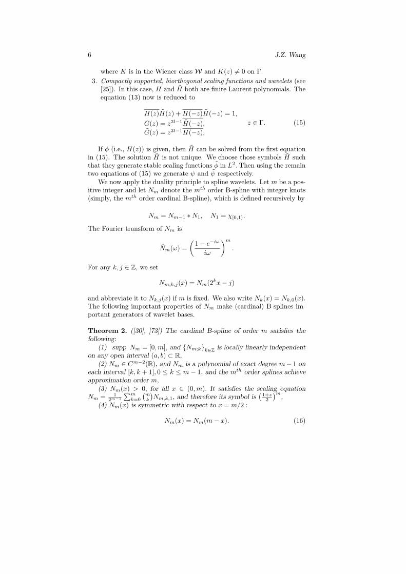
3. Compactly supported, biorthogonal scaling functions and wavelets (see[25]). In this case, H and H both are finite Laurent polynomials. Theequation (13) now is reduced to

H(z)H(z) + H(−z)H(−z) = 1,

G(z) = z2l−1H(−z),G(z) = z2l−1H(−z),

z ∈ Γ. (15)

If φ (i.e., H(z)) is given, then H can be solved from the first equationin (15). The solution H is not unique. We choose those symbols H suchthat they generate stable scaling functions φ in L2. Then using the remaintwo equations of (15) we generate ψ and ψ respectively.

We now apply the duality principle to spline wavelets. Let m be a pos-itive integer and let Nm denote the mth order B-spline with integer knots(simply, the mth order cardinal B-spline), which is defined recursively by

Nm = Nm−1 ∗N1, N1 = χ[0,1).

The Fourier transform of Nm is

Nm(ω) =(

1− e−iω

iω

)m

.

For any k, j ∈ Z, we set

Nm;k,j(x) = Nm(2kx− j)

and abbreviate it to Nk,j(x) if m is fixed. We also write Nk(x) = Nk,0(x).The following important properties of Nm make (cardinal) B-splines im-portant generators of wavelet bases.

Theorem 2. ([30], [73]) The cardinal B-spline of order m satisfies thefollowing:

(1) supp Nm = [0,m], and {Nm;k}k∈Z is locally linearly independenton any open interval (a, b) ⊂ R,

(2) Nm ∈ Cm−2(R), and Nm is a polynomial of exact degree m− 1 oneach interval [k, k + 1], 0 ≤ k ≤ m− 1, and the mth order splines achieveapproximation order m,

(3) Nm(x) > 0, for all x ∈ (0,m). It satisfies the scaling equationNm = 1

2m−1

∑mk=0

(mk

)Nm,k,1, and therefore its symbol is

(1+z2

)m,

(4) Nm(x) is symmetric with respect to x = m/2 :

Nm(x) = Nm(m− x). (16)


By Theorem 2, the cardinal B-spline of order m generates an MRA

· · · ⊂ Vm,−1 ⊂ Vm,0 ⊂ Vm,1 · · ·where Vm,0 = span{Nm,k}k∈Z.

Let {Wm,k}k∈Z be the corresponding wavelet subspace sequence suchthat Vm,k ⊕Wm,k = Vm,k+1, and Vm,k⊥Wm,k. A wavelet in Wm,0, whichgenerates the wavelet basis, is called a spline-wavelet.

The Euler-Frobenius polynomial (of order m− 1):

Em−1(z) =m−2∑

j=0

Nm(j + 1)zj , m ≥ 2

plays an important role in the construction of spline-wavelets. When m =2n, the Euler-Frobenius polynomial has an even degree and we rewrite itin a symmetric form:

Πn(z) = z−n+1E2n−1(z), n ≥ 1.

Theorem 3. [73] The Laurent polynomial Πn(z) has the following prop-erties.

(1) Πn(z) > 0,∀z ∈ Γ, and all of its 2n− 2 roots are positive. Assume{rj}2n−2

j=1 are all zeros of Πn(z) arranged increasingly:

0 < rn,1 < · · · < rn,n−1 < 1 < rn,n < · · · < rn,2n−2.

Thenrn,jrn,2n−1−j = 1. (17)

(2) It satisfies the following identity.

Pn(z)Πn(z) + Pn(−z)Πn(−z) = Πn(z2). (18)

where Pn(z) =(

1+z2

)n(

1+z−1

2

)n

.

Applying the duality principle and (18), we can construct various splinewavelets.1. Orthonormal spline-wavelets of the order n. [Lemarie (1988), Mallat

(1989)] Let the orthonormal scaling spline be denoted by N⊥n and the

corresponding wavelet denoted by Ψn. Then the symbol of N⊥n is

H⊥n (z) =

(1 + z

2

)n √Πn(z)√Πn(z2)

,

and the Fourier transform of the orthonormal wavelet Ψ is

Ψn(ω) = −e−iω/2H⊥n (−e−iω/2)N⊥

n (ω/2).

8 J.Z. Wang

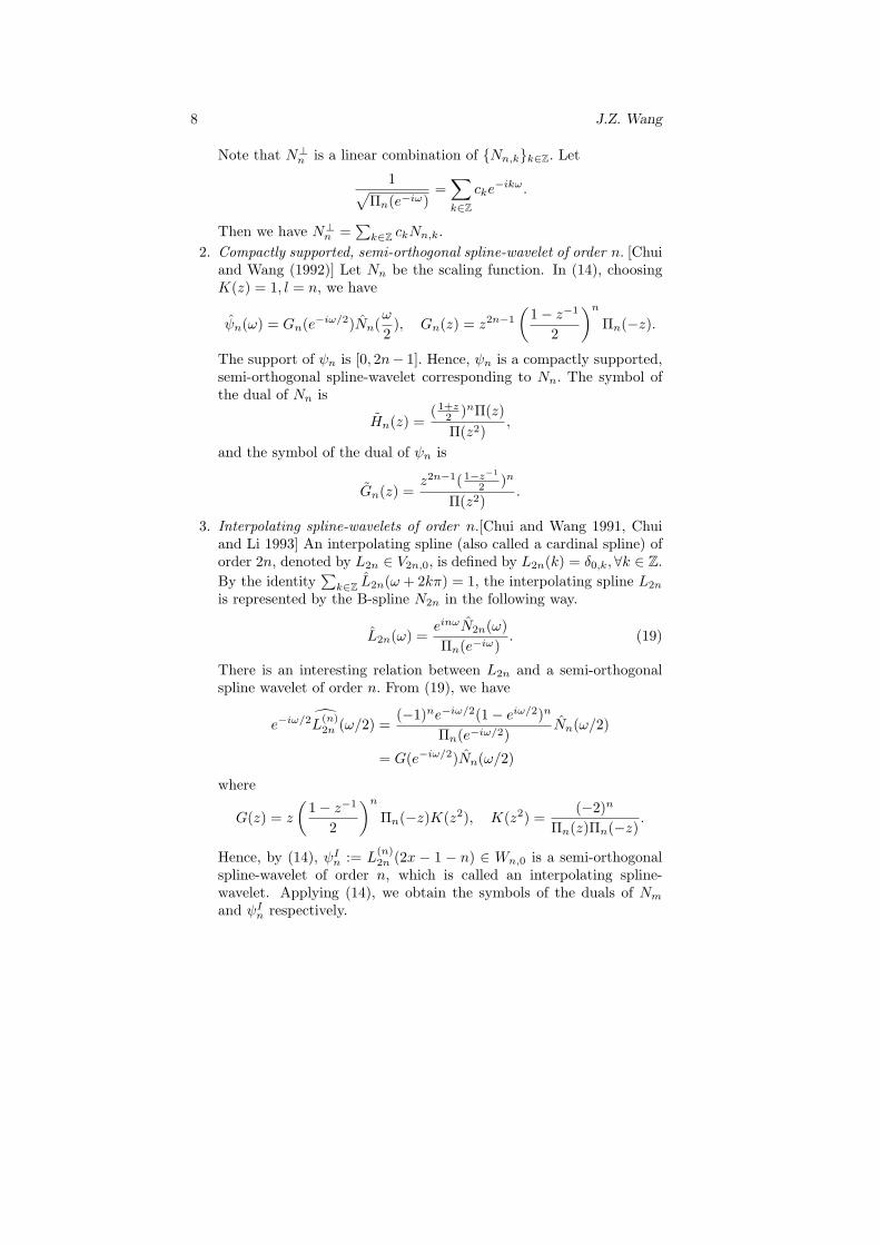
Note that N⊥n is a linear combination of {Nn,k}k∈Z. Let

1√Πn(e−iω)

=∑

k∈Zcke−ikω.

Then we have N⊥n =

∑k∈Z ckNn,k.

2. Compactly supported, semi-orthogonal spline-wavelet of order n. [Chuiand Wang (1992)] Let Nn be the scaling function. In (14), choosingK(z) = 1, l = n, we have

ψn(ω) = Gn(e−iω/2)Nn(ω

2), Gn(z) = z2n−1

(1− z−1

2

)n

Πn(−z).

The support of ψn is [0, 2n− 1]. Hence, ψn is a compactly supported,semi-orthogonal spline-wavelet corresponding to Nn. The symbol ofthe dual of Nn is

Hn(z) =( 1+z

2 )nΠ(z)Π(z2)

,

and the symbol of the dual of ψn is

Gn(z) =z2n−1( 1−z−1

2 )n

Π(z2).

3. Interpolating spline-wavelets of order n.[Chui and Wang 1991, Chuiand Li 1993] An interpolating spline (also called a cardinal spline) oforder 2n, denoted by L2n ∈ V2n,0, is defined by L2n(k) = δ0,k, ∀k ∈ Z.

By the identity∑

k∈Z L2n(ω + 2kπ) = 1, the interpolating spline L2n

is represented by the B-spline N2n in the following way.

L2n(ω) =einωN2n(ω)Πn(e−iω)

. (19)

There is an interesting relation between L2n and a semi-orthogonalspline wavelet of order n. From (19), we have

e−iω/2L(n)2n (ω/2) =

(−1)ne−iω/2(1− eiω/2)n

Πn(e−iω/2)Nn(ω/2)

= G(e−iω/2)Nn(ω/2)

where

G(z) = z

(1− z−1

2

)n

Πn(−z)K(z2), K(z2) =(−2)n

Πn(z)Πn(−z).

Hence, by (14), ψIn := L

(n)2n (2x − 1 − n) ∈ Wn,0 is a semi-orthogonal

spline-wavelet of order n, which is called an interpolating spline-wavelet. Applying (14), we obtain the symbols of the duals of Nm

and ψIn respectively.


§3. Computational of Spline-Wavelets

Wavelet bases are enable us to develop fast algorithms for decomposinga function into a wavelet series and recovering a function from its waveletseries, which are called Fast Wavelet Transform (FWT) algorithms andFast Inverse Wavelet Transform (FIWT) algorithms respectively. Let ψand ψ be a pair of dual wavelets. Then a function f ∈ L2 can be expandedas a wavelet series:

f =∑

j,k∈Zbj,kψj,k

or f =

∑

j,k∈Zbj,kψj,k

where

bj,k =∫ ∞

−∞f(t)ψj,k(t) dt

(bj,k =

∫ ∞

−∞f(t)ψj,k(t) dt

).

However, this expansion is not effective in computation. In scientific com-putation, we need to digitalize functions. Let φ and φ be the dual scalingfunctions corresponding to ψ and ψ respectively, and they generate thedual MRA {Vn} and {V }n. Assume φ, φ, ψ, and ψ are defined by (8), (9),(5) and (12) respectively. To discretize a function f ∈ L2, we choose asufficient large n such that ||f−fn|| is smaller than a tolerance ε, where fn

∈ Vn is a projection of f on Vn. Let cn = (cnm) be the coefficient sequenceof fn : fn =

∑m∈Z cnmφnm. The sequence cn, as the discrete represen-

tation of f, is the initial data for the fast wavelet transform. Assume wedecompose fn into

fn = f0 + g0 + · · ·+ gn−1, (20)

wherefj =

∑cj,kφj,k ∈ Vj

andgj =

∑dj,kψj,k ∈ Wj .

Write cj = (cj,k) and dj = (dj,k). Then FWT derives cj and dj fromcj+1,

FWT algorithm :

cj,k =√

2∑

h(l − 2k)cj+1,l

dj,k =√

2∑

g(l − 2k)cj+1,l(21)

and FIWT recovers cj+1 from cj and dj ,FIWT algorithm:

cj+1,l =√

2∑

h(l − 2k)cj,k +√

2∑

h(l − 2k)dj,k. (22)

10 J.Z. Wang

Let H, G, H, G be operators on l2 defined by

Ha(n) =√

2∑

k∈Zakh(n− 2k),

Ga(n) =√

2∑

k∈Zakg(n− 2k),

Ha(n) =√

2∑

k∈Zakh(k − 2n),

Ga(n) =√

2∑

k∈Zakg(k − 2n),

respectively. Then, the FWT and FIWT algorithms can be representedas

cj−1 = Hcj , dj−1 = Gdj

andcj = H∗cj−1 + G∗dj−1

respectively. Iterating FWT and FIWT algorithms, we complete mul-tilevel decomposition and recovering using the following decompositionpyramid algorithm

cnH→ cn−1

H→ cn−2H→ · · · H→ c0

G

↘G

↘G

↘G

↘dn − 1 dn − 2 · · · d0

, (23)

and recovering pyramid algorithm

c0H→ c1

H→ c2H→ · · · H→ cn

G

↗G

↗G

↗G

↗d0 d1 d2 · · ·

. (24)

Let us now analyze the FWT algorithm based on compactly supported,semi-orthogonal spline-wavelet of order m, in which the filters Hm andGm are infinite impulse responses (IIR). Hence, to apply the FWT algo-rithm, we have to truncate Hm to Hm,n = (hk}n

k=−n and Gm to Gm,n =(gk}n

k=−n. As an example, we analyze the truncate error of the filter Hm,n.

We estimate of the truncated error of the filter Hm,n by

En(Hm) = ||Hm − Hm,n||l2 .For any c ∈ l2, we have

||Hm ∗ c− Hm,n ∗ c||l2 ≤ En(Hm)||c||l2 , (25)

and the error estimate (25) is sharp. Charles and I (1992) obtain thefollowing estimate [23].


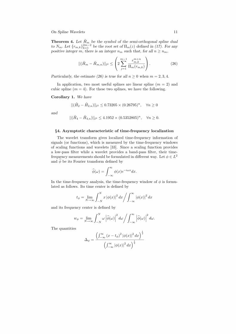
Theorem 4. Let Hm be the symbol of the semi-orthogonal spline dualto Nm. Let {rm,k}2m−2

k=1 be the root set of Πm(z) defined in (17). For anypositive integer m, there is an integer nm such that, for all n ≥ nm,

||(Hm − Hm,n)||l2 ≤2

m−1∑

j=1

rm+nm,k

Πm(rm,k)

. (26)

Particularly, the estimate (26) is true for all n ≥ 0 when m = 2, 3, 4.

In application, two most useful splines are linear spline (m = 2) andcubic spline (m = 4). For these two splines, we have the following.

Corollary 1. We have

||(H2 − H2,n)||l2 ≤ 0.73205× (0.26795)n, ∀n ≥ 0

and||(H4 − H4,n)||l2 ≤ 4.1952× (0.5352805)n, ∀n ≥ 0.

§4. Asymptotic characteristic of time-frequency localization

The wavelet transform gives localized time-frequency information ofsignals (or functions), which is measured by the time-frequency windowsof scaling functions and wavelets [33]. Since a scaling function providesa low-pass filter while a wavelet provides a band-pass filter, their time-frequency measurements should be formulated in different way. Let φ ∈ L2

and φ be its Fourier transform defined by

φ(ω) =∫ ∞

−∞φ(x)e−iωxdx.

In the time-frequency analysis, the time-frequency window of φ is formu-lated as follows. Its time center is defined by

tφ = limN→∞

∫ N

−N

x |φ(x)|2 dx

/∫ ∞

−∞|φ(x)|2 dx

and its frequency center is defined by

wφ = limN→∞

∫ N

−N

ω∣∣∣φ(ω)

∣∣∣2

dω

/∫ ∞

−∞

∣∣∣φ(ω)∣∣∣2

dω.

The quantities

∆φ =

(∫∞−∞ (x− tφ)2 |φ(x)|2 dx

) 12

(∫∞−∞ |φ(x)|2 dx

) 12

12 J.Z. Wang

and

∆φ =

(∫∞−∞ (ω − ωφ)2

∣∣∣φ(ω)∣∣∣2

dω

) 12

(∫∞−∞

∣∣∣φ(ω)∣∣∣2

dω

) 12

are called the time and frequency localization radii of φ. If both ∆φ and∆φ are finite, we say that φ is a window function and denote the measureof its time-frequency window by

M(φ) = ∆φ∆φ .

The following uncertainty principle is well known.

Theorem 5. If φ is a window function, then

M(φ) ≥ 12

and equality holds if and only if

φ = kGσ(x− µ), k 6= 0, σ > 0, µ ∈ R,

where

Gσ(x) =1√2πσ

e−x2

2σ2

is a Gaussian function.

Note that the Gaussian function Gσ is not a scaling function.Because a wavelet ψ satisfies ψ(0) = 0, from the point of view of

signal processing, it is a bandpass filter. As a bandpass filter, ψ treatspositive and negative frequency bands separately. Therefore, the notionof the frequency window of a bandpass filter ψ has to be modified. Moreprecisely, we have to consider two frequency centers for a bandpass filterψ. The positive frequency center is defined by

ω+

ψ=

∫∞0

ω∣∣∣ψ(ω)

∣∣∣2

dω

∫∞0

∣∣∣ψ(ω)∣∣∣2

dω

and the negative frequency center is defined by

ω−ψ

=

∫ 0

−∞ ω∣∣∣ψ(ω)

∣∣∣2

dω

∫ 0

−∞

∣∣∣ψ(ω)∣∣∣2

dω.


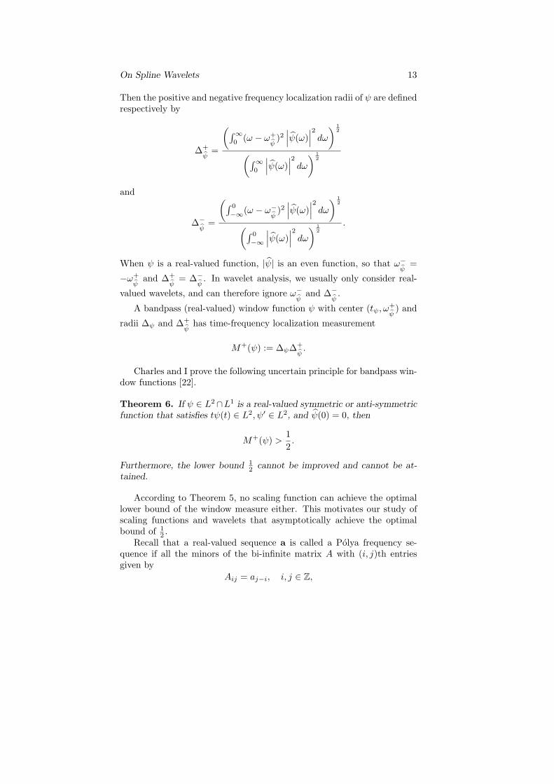
Then the positive and negative frequency localization radii of ψ are definedrespectively by

∆+

ψ=

(∫∞0

(ω − ω+

ψ)2

∣∣∣ψ(ω)∣∣∣2

dω

) 12

(∫∞0

∣∣∣ψ(ω)∣∣∣2

dω

) 12

and

∆−ψ

=

(∫ 0

−∞(ω − ω−ψ

)2∣∣∣ψ(ω)

∣∣∣2

dω

) 12

(∫ 0

−∞

∣∣∣ψ(ω)∣∣∣2

dω

) 12

.

When ψ is a real-valued function, |ψ| is an even function, so that ω−ψ

=

−ω+

ψand ∆+

ψ= ∆−

ψ. In wavelet analysis, we usually only consider real-

valued wavelets, and can therefore ignore ω−ψ

and ∆−ψ

.

A bandpass (real-valued) window function ψ with center (tψ, ω+

ψ) and

radii ∆ψ and ∆+

ψhas time-frequency localization measurement

M+(ψ) := ∆ψ∆+

ψ.

Charles and I prove the following uncertain principle for bandpass win-dow functions [22].

Theorem 6. If ψ ∈ L2∩L1 is a real-valued symmetric or anti-symmetricfunction that satisfies tψ(t) ∈ L2, ψ′ ∈ L2, and ψ(0) = 0, then

M+(ψ) >12.

Furthermore, the lower bound 12 cannot be improved and cannot be at-

tained.

According to Theorem 5, no scaling function can achieve the optimallower bound of the window measure either. This motivates our study ofscaling functions and wavelets that asymptotically achieve the optimalbound of 1

2 .Recall that a real-valued sequence a is called a Polya frequency se-

quence if all the minors of the bi-infinite matrix A with (i, j)th entriesgiven by

Aij = aj−i, i, j ∈ Z,

14 J.Z. Wang

(where a = {aj} and an := 0 if n is not in the index set of a,) are non-negative, that is,

A

(i1, · · · , ipj1, · · · , jp

):= det

k,`=1,···pAikj`

≥ 0,

for all integers p ≥ 1 and i1 < · · · < ip, j1 < · · · < jp. (See [60] forthe properties of Polya frequency sequences.) If a is a finite sequence, itslength will be denoted by |a|.

Now let φ ∈ L1 be a scaling function with the mask a, and define

Bφ

(e−iω

)=

∑

n∈Z

∣∣∣φ(ω + 2nπ)∣∣∣2

. (27)

Assume its corresponding semi orthogonal wavelet ψ is defined by

ψ(ω) = Cψe−i ω2 a

(−e−i ω2)Bφ

(−e−i ω2)φ

(ω

2

), (28)

where Cψ is a positive constant so chosen that ‖ψ‖∞ = 1.If a is a symmetric finite Polya frequency sequence, we will call φ a

stoplet and ψ a cowlet, respectively. We denote the standard deviation ofφ by

σ =(∫ ∞

−∞φ(x) (x− tφ)2 dx

) 12

. (29)

Charles and I reveal that the time-frequency localization of semi- or-thogonal spline-wavelets is asymptotically optimal. On the contract, thesize of time-frequency window of orthonormal two-scaling functions andwavelets grows to infinity as the smoothness increases. For a scaling func-tion of spline-type, we have the following [21].

Theorem 7. For each n, let an = {anj }kn

j=0 be a finite symmetric Polyafrequency sequence with symbol

an(z) =(

1 + z

2

)n

pn(z), (30)

for some polynomial pn(z) that satisfies pn(1) = 1, pn(−1) 6= 0 anddegpn ≤ Cn, where C is a positive constant independent of n. Let φn

be the stoplet determined by an and σn be its standard variation. Then(1) limn→∞ σn = +∞;(2) the following limits hold:

limn→∞

∥∥∥∥φn

(ω

σn

)ei knω

2σn − e−ω22

∥∥∥∥Lp

= 0, 1 ≤ p < ∞, (31)


and

limn→∞

∥∥∥∥σnφn

(σnx +

kn

2

)− 1

2πe−

x22

∥∥∥∥Lq

= 0, 2 ≤ q < ∞; (32)

(3) furthermore,

limn→∞

1σn

∆φn = limn→∞

σn∆φn=

1√2, (33)

so that

limn→∞

M(φn) =12. (34)

For a semi-orthogonal wavelet of spline-type, we have the following[22].

Theorem 8. Let ψn be the cowlets corresponding to the stoplets φn asin Theorem 7. Then

(1) for each n, there is a unique ωn in (0,∞), at which the function

|ψn(ω)| attains its absolute maximum value;

(2) π ≤ ωn ≤ 2π, and τn :=√|ψ′′n(ωn)| → ∞ as n →∞;

(3) the following limits hold:

limn→∞

∥∥∥∥eiω2τn ψn

(ω

τn

)− e−

(ω−ωnτn)2

2

∥∥∥∥Lp(0,+∞)

= 0, 1 ≤ p < ∞, (35)

so that for even n,

limn→∞

∥∥∥∥τnψn

(τnx +

12

)− 1

2πcos (τnωnx) e−

x22

∥∥∥∥Lq

= 0, 2 ≤ q < +∞,

(36)and for odd n,

limn→∞

∥∥∥∥τnψn

(τnx +

12

)− 1

2πsin(τnωnx)e−

x22

∥∥∥∥Lq

= 0, 2 ≤ q < +∞;

(37)(4) furthermore,

limn→∞

1τn

∆ψn = limn→∞

τn∆+

ψn

=1√2, (38)

so that

limn→∞

M+ (ψn) =12. (39)

As an application of Theorems 7 and 8, we have the following corollar-ies for B-spline and for the compactly supported, semi-orthogonal spline-wavelet.

16 J.Z. Wang

Corollary 2. We have

limn→∞

∥∥∥∥∥Nn

(ω√

12√n

)e√

3nωi − e−ω22

∥∥∥∥∥Lp

= 0, 1 ≤ p < ∞, (40)

limn→∞

∥∥∥∥√

n

12Nn

(√n

12x +

n

2

)− 1

2πe−

x22

∥∥∥∥Lq

= 0, 2 ≤ q < ∞. (41)

Furthermore,

limn→∞

√12n

∆Nn= lim

n→∞

√n

12∆

Nn=

1√2, (42)

so that

limn→∞

M(Nn) =12. (43)

Corollary 3. Let ψn be the compactly supported, semi-orthogonal splinewavelet corresponding to Nn. Let ω0(≈ 1.6367π) be the unique value in

(0,∞), at which the function C(ω) :=8(1− cos ω)ω(2π − ω)2

attains its absolute

maximum value. Set α =√

1C(ω0)

|C ′′(ω0)|(≈ 0.3745). Then for 1 ≤ p <∞,

limn→∞

∥∥∥∥ei ω2α√

n ψNn

(ω

α√

n

)− e−

(ω−αω0√

n)2

2

∥∥∥∥Lp(0,+∞)

= 0, (44)

and therefore, for even n and 2 ≤ q < +∞,

limn→∞

∥∥∥∥α√

nψNn

(α√

nx +12

)− 1

2πcos

(αω0

√nx

)e−

x22

∥∥∥∥Lq

= 0, (45)

and for odd n and 2 ≤ q < +∞,

limn→∞

∥∥∥∥α√

nψNn

(α√

nx +12

)− 1

2πsin

(αω0

√nx

)e−

x22

∥∥∥∥Lq

= 0. (46)

Moreover,

limn→

1α√

n∆ψNn

= limn→∞

α√

n∆+

ψNn

=1√2, (47)

so that

limn→∞

M+(ψNn) =12. (48)

We remark that (40), (41) and (44)–(46) were already established bythe authors of [74] in a different way.

For orthonormal scaling function and wavelets, we have the followingremarkable results [20].


Theorem 9. Let φn be the orthonormal scaling function with the symbol

P (z) =(

1 + z

2

)n

Sn(z),

where |Sn(e−iω)| ≤ C2n| sinn(

ω2

) |, π2 ≤ |ω| ≤ π. Let ψn be the corre-

sponding orthonormal wavelet. Then

limn→∞

|| |φn| − χ[−π,π]||L2 = 0,

limn→∞

∆φn=

π√3,

limn→∞

∆φn= ∞.

and

limn→∞

|| |ψn| − χ[−2π,−π]∪[π,2π]||L2 = 0,

limn→∞

∆+

ψn=

π

2√

3,

limn→∞

∆ψn = ∞.

Consequently, the sizes of the time-frequency windows of both φn and ψn

tend to infinity:

limn→∞

M(φn) = ∞, limn→∞

M+(ψn) = ∞.

Recently, the uncertainty principle for scaling functions and waveletsare discussed in various angles by Goh, Goodman, Lee, and other authorsin the papers [5], [38], [39], [40], [42], and their references.

§5. Sub-band code and general sample theory

In signal transmission, the sub-band coding is a main method formultiple-channel synchronized transmission. In multi-channel transmis-sion, a signal is decomposed into several sub-signal by its frequency dis-tribution, where each sub-signal has a certain frequency band. The corre-sponding coding method is called sub-band coding. The sub-band codingmust be consistent of the sampling method. On the other hand, an impor-tant purpose of sub-band coding is to achieve the lower bite rate. Wavelettheory provides a useful tool for the study of sub-band coding.

In signal processing, all continuous-time signals f(t) are often consid-ered to be real-valued and band-limited. A signal f ∈ L2 is said to beband-limited if supp f ⊂ [−B, B], where B > 0. Assume f is a real-valuedfunction. Then supp f is a symmetric set (with respect to the origin) on

18 J.Z. Wang

R, i.e., x ∈ supp f ⇐⇒ −x ∈ supp f . Therefore, in the study we can usethe bounded set

supp+f :=(supp f

)∩ [0,∞)

to substitute supp f . The well-known sampling theorem allows us to re-cover the continuous-time band-limited signal f(t) from a certain sampleset f(kT ), t > 0, by using the sampling function

φ(t) = sinc t :=sin πt

πt.

A precise statement of this theorem is the following [59].

Theorem 10 (Shannon Sampling Theorem) A continuous-time andreal-valued band-limited signal f(t) with

supp+f ⊂ [0, 2πσ] (49)

has the infinite series representation

f(t) =∞∑

k=−∞f(kT )sinc (2σ(t− kT ))

where T = 12σ .

In signal processing, we always assume 2πσ in (49) is the least upperbound (lub) of supp+f . Thus, we call σ the highest band of f. Since theset

{sinc (2σ(t− kT ))}k∈Z

is linearly independent, the sampling theorem asserts that to completelyrecover a signal f(t) from its sample set {f(k/µ)}, the sampling rate)µ (also called the sampling frequency) must satisfy µ ≥ 2σ, where 2σis the smallest sampling rate for the completely recovering of f , called theNyquist frequency or Nyquist rate of f(t).

For example, to sample a speech signal with highest band 4 kHz, thesampling rate must be at least 8 kHz to avoid distortion; and the samplingrate of high-quality music signals (with highest band 22.05 kHz) is at least44.1 kHz. Then 8 kHz and 44.1 kHz are their Nyquist rates.

However, most of speech signals do not cover all bands in [0, σ], butonly a collection of sub-intervals in [0, σ]. Assume a signal f has a positivelowest band µ and the highest band ν, i.e.,

supp+f ⊂ [2πµ, 2πν]. (50)

Then σ := ν − µ is called the bandwidth of f(t). For such a bandpasssignal, if it is sampled by using the sample method in Theorem 10, then


its Nyquist rate is 2σ2. However, if σ1/σ is an integer, the sampling ratecan be reduced from the (standard) Nyquist frequency 2ν to 2σ (see [59]).As we will show later, the rate 2σ is the smallest rate for the completelyrecovering. For this reason, 2σ is also called the Nyquist frequency forbandpass signals (when µ/σ is an integer). When µ/σ is not an integer,it was shown in [61] that the smallest sampling rate for complete recoveryof f(t) is given by 2σm,

σm = σ1 + µ/σ

1 + bµ/σcwhere the notation bxc stands for the integer part of x. We call σm/ν (≤ 1)the bit rate of the coding method for f, which samples f using its band-pass property (50).

The sampling theorem for bandpass signals has been applied in thestudy of sub-band coding (see [28], [29], [50], [75]), and is often considered afundamental result for multiple-channel synchronized transmission. Sincethe signals to be transmission are usually sampled by {f(k/2ν)}, where νis the highest band of f. In multiple-channel synchronized transmission,we need to do the following. (1) To determine the nearly lowest samplingrate of a signal f. (2) To extract a sub-sampling data of {f(k/2ν)} thatachieves the rate. (3) To develop a fast algorithm that recovers f fromthe sub-sampling data of the signal. To explain the tasks more clearly, wegive the following.

Definition 3. A sub-band decomposition of a bandlimited signal f(t) isthe following.

f(t) =n∑

k=1

fk(t), (51)

where supp+ fk ⊂ [2πµk, 2πνk],

0 ≤ µ1 < ν1 ≤ µ2 < ν2 ≤ · · · ≤ µn < νn , (52)

and µk and νk satisfy the sub-band decomposition conditions:(i) µk/σk, k = 1, . . . , n, are integers;(ii) σk/σ`, k, ` = 1, . . . , n, are rationales.

If µk and νk in (52) are the lowest and highest bands of fk, thenCondition (i) ensures that the smallest sampling rate of each sub-band isequal to its Nyquist frequency, and Condition (ii) ensures the existenceof some positive integer N and some σ > σk, k = 1, . . . , n, such thatNσk/σ, k = 1, . . . , n, are integers.

Definition 4. Let S = {rk}k∈Z, r ∈ (0,∞), V = {λk + τ}k∈Z, λ ∈(0,∞), τ ∈ R, and V ⊂ S. Then we say the set V has a compressionrate λ/r with respect to S.

20 J.Z. Wang

We have the following .

Theorem 11. [24] If f has a sub-band decomposition (51) and f is sam-pled by S := {f(k/2vn)}k∈Z, then (1) each fk can be sampled by a subsetSk ⊂ S with the compression rate νn/σk (or the bit rate σk/νk). (2)Sk ∩ Sj = ∅, k 6= j.

This property allows the feasibility of bit allocation for each sub-bandsignal (see [51]).

To complete recover a band-limited signal f(t) with sub-band decom-position given in (51), we only need to recover each fk(t), which has thesampling rate ≤ 2σk = 2(νk−µk). Then f can be recovered by a sampling(or coding) rate

2σs := 2n∑

k=1

σk.

We call 2σs the sub-band sampling rate (or coding rate) corresponding tothe sub-band decomposition (51). It is also known that if fk has the exact(positive) support [µk, νk], i.e., supp+ fk = [2πµk, 2πνk], then its Nyquistrate is equal to 2σk. Therefore, we give the following.

Definition 5. Let

σf =mes(supp+ f)

π,

where the notation “mes” stands for the Lebesgue measure. Then 2σf iscalled the theoretical Nyquist frequency of a band-limited signal f(t).

It is obvious that for each sub-band decomposition of f, its sub-bandcoding rate is no less than its theoretical Nyquist frequency 2σf . Fromthe point of view of signal transmission, a good sub-band sampling shouldachieve a sampling rate as close to 2σf as possible. Charles and I in [24]apply Shannon wavelet packets in the study of subband-coding.

According to [49], the function φ(t) = sinc t is called the Shannonscaling function and the function ψ(t) = 2sinc(2t) − sinc t is called theShannon wavelet. Let

· · ·V−2 ⊂ V−1 ⊂ V0 ⊂ V1 ⊂ V2 ⊂ · · · ,

be the MRA generated by φ(t) :

Vn = {f ∈ L2 : suppf ⊂ [−2nπ, 2nπ]}.Let {Wn}n∈Z be the corresponding wavelet subspaces generated by ψ.Then Wn ⊥ Vn, Wn + Vn = Vn+1. We have

φ(ω) = χ[−π,π)(ω)

ψ(ω) = χ[−2π,−π)∪[π,2π)(ω).


Let p0(ω) be the 2π-periodic function:

p0(ω) ={

1, ω ∈ [−π2 , π

2 ),0, ω ∈ [−π,−π

2 ) ∪ [π2 , π),

and writep1(ω) = p0(ω + π).

Then, we have

φ(ω) = p0(ω/2)φ(ω/2),

ψ(ω) = p1(ω/2)φ(ω/2).

The Shannon wavelet packets can be constructed as follows. Write{

µ0(t) = φ(t),µ1(t) = ψ(t).

Then, we have {µ0(ω) = p0(e−iω/2)µ0(ω/2),µ1(ω) = p1(e−iω/2)µ0(ω/2).

For even n, we set{

µ2n(ω) = p0(e−iω/2)µn(ω/2),µ2n+1(ω) = p1(e−iω/2)µn(ω/2),

and for odd n, set{

µ2n(ω) = p1(e−iω/2)µn(ω/2)µ2n+1(ω) = p0(e−iω/2)µn(ω/2),

Then the collection {µl}∞l=0 is a family of Shannon wavelet packets.It can be easily verified that

µl(t) = (l + 1)sinc ((l + 1)t)− lsinc (lt) ,

or, equivalently,

µl = χ[−(l+1)π,−lπ)∪[lπ,(l+1)π), l = 0, 1, 2, · · · .

Writeµl,j,k(t) = 2j/2µl(2jt− k).

We have

µl,j,k(ω) = ei2−jkωχ[−2j(l+1)π,−2j lπ)∪[2j lπ,2j(l+1)π).

22 J.Z. Wang

Define

U lj = closL2 span {2j/2µl(2jt− k) : k ∈ Z}, j ∈ Z, l ∈ Z+.

The each function in U lj is a bandpass signal with lowest band 2j−1l,

highest band 2j−1(l+1), and bandwidth 2j−1. In addition, it also satisfiesthe sub-band coding condition (i). For any n = 0, 1, 2, · · · , we have

Unj+1 = U2n

j ⊕ U2n+1j , U2n

j ⊥U2n+1j , j ∈ Z.

Therefore, for j ≥ 1 and k ≥ 0, we have

Wj = U2k

j−k ⊕ U2k+1j−k ⊕ · · · ⊕ U2k+1−1

j−k .

Let Ij,l = [2j lπ, 2j(l + 1)π]. Let Λ and Γ be two subsets of the integer set.Then the set {Ij,l : j ∈ Λ, l ∈ Γ} forms a dyadic partition of R+ := [0,∞)if ∪j∈Λ,l∈ΓIj,l = R+ and mes (Ij,l ∩ Ij′,l′) = 0, (j, l) 6= (j′, l′). It can beproved that if {Ij,l : j ∈ Λ, l ∈ Γ} is a dyadic partition of R+, then the setof {ψj,l,k : j ∈ Λ, l ∈ Γ, k ∈ Z} is an orthonormal basis of L2 and L2 =⊕j∈Λ,l∈ΓU l

j . Therefore, if f ∈ Un0 , that is, supp+f ⊂ I0,n := [nπ, (n+1)π],

thenf(t) =

∑

k∈Z

f(k)µn,0,k(t).

By the nice properties of Shannon wavelet packet in the frequency domain,we can prove the following [24].

Theorem 12. Let f be a bandlimited signal with theoretical Nyquistfrequency 2σf . Then for any λf > σf , there is a sub-band decomposition(51) of f, with sub-band coding rate no greater than 2λf . Furthermore,the sub-band coding rate of any sub-band decomposition of f is at least2σf .

Theorem 13. Let f be a bandlimited signal with highest band σ andtheoretical Nyquist frequency σf . Then for any σ > σf ,

(1) there exists a sub-band decomposition of f that achieves bit-ratecompression ratio larger than σ/σ,

(2) the sub-band coding can be realized by a Shannon wavelet packet.

The Shannon wavelet packet introduced above has a primary band-width 1/2 (i.e., both φ and ψ have bandwidth 1/2). Therefore, eachfunction in the subspace U l

j has the dyadic bandwidth 2j−1. In applica-tion we need to construct the Shannon wavelet packets with primary banddifferent from 2j . To do this, for a positive number ν /∈ 2j , we define

φν(t) = (2ν)1/2φ(2νt), ψν(t) = (2ν)1/2ψ(2νt).


Then both φν(t) and ψν(t) have bandwidth ν. Let

φνj,k(t) = 2j/2φν(2jt− k

2ν) =

(2(j+1)/2ν1/2φ(2j+1νx− t)

),

ψνj,k(t) = 2j/2ψν(2jt− k

2ν) =

(2(j+1)/2ν1/2ψ(2j+1νt− k)

).

Then {ψνj,k : j, k ∈ Z} creates the Shannon wavelet packet has primary

band ν. The Shannon wavelet library therefore can be constructed as fol-lows. Denote the Shannon wavelet packets with the primary band ν byPν . Two positive numbers ν and µ are said to be binarily similar if thereexists an integer j such that ν = 2jµ. Let B ⊂ R be the set of all numbersthat are not binarily similar to each other. Then

{Pν : ν ∈ B}constitutes a Shannon wavelet library.

We now have two ways to do the sub-band decomposition for a signalf.

1. We use a single Shannon wavelet packet, say Pν , in the library for sub-band decomposition. In this case, the decomposition always satisfiesthe sub-band coding conditions (i) and (ii). In addition, all sub-bandfunctions of a sub-band coding obtained in this way are synchronic,and therefore, no additional code is needed for synchronized transmis-sion.

2. We use the whole Shannon wavelet library for sub-band decomposi-tion. We may decompose a signal f(t) into sub-band signals usingseveral packets:

f(t) =m∑

l=1

nl∑

k=1

flk(t),

where flk(t) and fl′k′(t) have different primary bands if and only ifl 6= l′. Thus, the signal f is decomposed by using m different waveletpackets Pνl , 1 ≤ l ≤ m. The decomposition is a sub-band decompo-sition if all the ratios νk/νk′ , 1 ≤ k, k′ ≤ m, are rational numbers. Inthis case, additional code may be needed for synchronized transmis-sion.

References

1. A. Aldroubi and M. Unser, Families of multiresolution and waveletspaces with optimal properties, Numer. Funct. Anal. Optimiz.14(1993), 417-446.

2. G. A. Battle, Wavelets of Federbush-Lemarie type, J. Math. Phys. 34(1993), 1095-2002.

24 J.Z. Wang

3. G. Beylkin, R. R. Coinfman, and V. Rokhlin, Fast wavelet transformsand numerical algorithms I, Comm. Pure and Appl. Math. 44 (1991),141-183.

4. W. Cai and J. Wang, Adaptive multiresolution collocation methodsfor initial boundary value problems of nonlinear PDEs, SIAM. Numer.Anal. 33 (1996), 937-970.

5. L. H. Y. Chen, T. N. T. Goodman, and S. L. Lee, Asymptotic normalityof scaling functions, SIAM J. Math. Anal. 36 (2004), 323-346.

6. C. K. Chui, An Introduction to Wavelets, Academic Press, Boston,1992.

7. C. K. Chui, editor. Wavelets: A Tutorial in Theory and Applications,Academic Press, New York, 1992.

8. C. K. Chui, J. W. He, and J. Stoeckler, Nonstationary tight waveletframes, I and II: Appl. Comput. Harmon. Anal. 17 (2004), 141-197.

9. C. K. Chui, J. W. He, J. Stoeckler, and Q. Sun, Compactly supportedtight affine frames with integer dilations and maximum vanishing mo-ments, Advanced Computational Mathematics 18 (2003), 159-187.

10. C. K. Chui, J. W. He, and J. Stoeckler, Compactly supported tightand sibling frames with maximum vanishing moments, Appl. Comput.Harmon. Anal. 13 (2002), 224-262.

11. C. K. Chui, J. W. He, and J. Stoeckler, Tight frames with maximumvanishing moments and minimum support, in Approximation TheoryX, C.K. Chui, L.L. Schumaker, and J. Stoeckler, eds., Vanderbilt Uni-versity Press, Nashville, (2002), 187-206.

12. C. K. Chui and J. W. He, Compactly supported tight frames associatedwith refinable functions, Appl. Comput. Harmon. Anal. 8 (2000), 293-319.

13. C. K. Chui and C. Li, Dyadic affine decompositions and functionalwavelet transforms, SIAM J. Math. Anal. 27 No.3 (1996), 865-890.

14. C. K. Chui, and J. Lian, A study of orthonormal multiwavelets, J.Applied Numerical Mathematics 20 (1996), 272-298.

15. C. K. Chui, E. Quak, Wavelets on a bounded interval, in NumericalMethods of Approximation Theory, Volume 9, D. Braess and L. L. Schu-maker (eds.), International Series of Numerical Mathematics, Volume105, Birkhuser, Basel, (1992), 53-75.

16. C. K. Chui and J. Z. Wang, A cardinal spline approach to wavelets,Proc. Amer. Math. Soc. 113 (1991), 785-793.

17. C. K. Chui and J. Z. Wang, On compactly supported spline waveletsand a duality principle, Trans. Amer. Math. Soc. 330 (1992), 903-915.

18. C. K. Chui and J. Z. Wang, A general framework of compactly sup-ported splines and wavelets, J. Approx. Theory 71 (1992), 263-304.


19. C. K. Chui and J. Z. Wang, An analysis of cardinal spline-wavelets, J.Approx. Theory 72 (1993), 54-68.

20. C. K. Chui and J. Z. Wang, High-order orthonormal scaling functionsand wavelets give poor time-frequency localization, J. Fourier Anal.and Appl. 2 (1996), 415-426.

21. C. K. Chui and J. Z. Wang, A study of compactly supported scalingfunctions and wavelets, in “Wavelets, Images, and Surface Fitting”,Ed. P. Laurent, M. L. Mehaute, L.L. Schumaker, and A K Peters,Wellesley, MA, (1994), 121-140.

22. C. K. Chui and J. Z. Wang, A study of asymptotically optimal time-frequency localization by scaling functions and wavelets,Annals of Nu-mer. Math. 4 (1997), 193-216.

23. C. K. Chui and J. Z. Wang, Computational and algorithmic aspects ofcardinal spline wavelets, Approx. and Its Appl. 2 (1993), 53-75.

24. C. K. Chui and J. Z. Wang, Shannon Wavelet Approach to Sub-BandCoding, International Journal of Wavelets, Multiresolution and Infor-mation Processing 1 (2003), 233-242.

25. A. Cohen, I. Daubechies, and J. C. Feauveau, Biorthogonal basisof compactly supported wavelets, Comm. Pure. and Appl. Math. 45(1992), 485-560.

26. A. Cohen, I. Daubechies, B. Jawerth, and P. Vial, Multiresolution anal-ysis, wavelets, and fast algorithms on an interval, Comptes Rendus AcadSci. Paris A 316 (1993) 417-421.

27. A. Cohen, N. Dyn, and D. Levin, Stability and inter-dependence ofmatrix subdivision schemes, in “Advanced Topics in Multivariate Ap-proximation ”, Eds: F. Fontanelle, K. Jetter and L. Schumaker, WorldSci. Publishing Co. (1996), 1-13.

28. R. E. Crochiere, Sub-band coding, Bell System Tech. J. (1981), 1633-1654.

29. R. E. Crochiere, R. V. Cox, and J. D. Johnston, Real time speechcoding, IEEE Trans. on Communications (1982), 621-634.

30. C. de Boor, A Practical Guide to Splines, Springer-Verlag, 1978.31. C. de Boor, Total positivity of the spline collocation matrix, Ind. Univ.

J. Math. 25 (1976), 541-551.32. I. Daubechies, Ten Lectures on Wavelets, CBMS-NSF Series in Appl.

Math. #61, SIAM, Philadelphia, 1992.33. I. Daubechies, The wavelet transform, time-frequency localization and

signal analysis, IEEE Trans. Inform. Theory 36 (1990), 961-1005.34. I. Daubechies, B. Han, A. Ron, and Z. W. Shen, Framelets: MRA-

based constructions of wavelet frames, Appl. Comput. Harmon. Anal.14 (2003), 1-46.

26 J.Z. Wang

35. D. L. Donoho, Interpolating wavelet transform, preprint, 1992.36. G. Donovan, J. S. Geronimo, and D. P. Hardin, Interwining multires-

olution analyses and the construction of pieewise polynomial wavelets,SIAM J. Math. Anal. 27 (1996), 1791-1815.

37. G. Donovan, J. S. Geronimo, D. P. Hardin, and P. R. Massopust, Con-struction of orthogonal wavelets using fractal interpolation functions,SIAM J. Math. Anal. 27 (1996), 1158-1192.

38. S. S. Goh and T. N. T. Goodman, Uncertainty principle and asymptoticbehavior, Appl. Comput. Harmon. Anal. 16 (2004), 19-43.

39. S. S. Goh and C. A. Micchelli, Uncertainty principle in Hilbert space,J. Fourier Anal. Appl. 8 (2002), 335-373.

40. S. S. Goh and C. H. Yeo, Uncertaity products of local periodic wavelets,Adv. Comput. Math. 13 (2000), 319-333.

41. T. N. T. Goodman, and S. L. Lee, Wavelets of multiplicity r, Trans.Amer. Math. Soc. 342 (1994), 307-324.

42. T. N. T. Goodman and S. L. Lee, Asymptotic optimality of wavelets,preprint.

43. T. N. T. Goodman and C. A. Micchelli, On refinement equations deter-mined by Polya frequency sequences, SIAM J. Math. Anal. 23 (1992),766-784.

44. B. Han, and R. Q. Jia, Multivariate refinement equations and subdivi-sion schemes, SIAM J. Math. Anal. 29 (1998), 1177-1199.

45. B. Han and Z. W. Shen, Wavelet with short support, (2003), preprint.46. B. Han and Z. W. Shen, Wavelet from the loop scheme, J. Fourie, Anal.

and Appl., to appear.47. W. He and M. J. Lai, Construction of trivariate compactly supported

biorthogonal box wavelets, J. Approx. Theory, 120 (2003), 1-19.48. W. He and M. J. Lai, Construction of bivariate compactly supported

biorthogonal box spline wavelets with arbitrarily high regularities,Appl. Comput. Harmon. Anal. 6 (1999), 53-74.

49. E. Hernandez and G. Weiss, A First Course on Wavelets, CRC Press,(1996).

50. C. D. Heron, R. E. Crochiere, and R. V. Cox, A 32-band sub-band/transform coder interpolating vector quantization for dynamicbit allocation, Proc. ICASSP (1983), 1276-1279.

51. N. S. Jayant and P. Noll, Digital Coding of Waveforms: Principles andApplications to Speech and Video, Prentice Hall (1984).

52. R. Q. Jia and C. A. Micchelli, On linear independence for integer trans-lates of a finite number of functions, Proc. Edinburgh Math. Soc. 36(1992), 69-85.

53. R. Q. Jia, S. D. Riemenschneider, and D. X. Zhou, Smoothness of


multiple refinable functions and multiple wavelets, SIAM Journal ofMatrix Analysis and Applications 21 (1999), 1-28.

54. R. Q. Jia, S. D. Riemenschneider and D. X. Zhou, Approximation bymultiple refinable functions, Canadian J. Math. 49 (1997), 944-962.

55. R. Q. Jia and J. Z. Wang, Stability and linear independence associatedwith wavelet decompositions, Proc. Amer. Math. Soc. 117 (1993), 1115-1124.

56. Q. T. Jiang, On the design of multifilter banks and orthogonal multi-wavelet bases, IEEE Trans. on Signal Proc. 46 (1998), 3292-3303.

57. Q. T. Jiang, Construction of biorthogonal multiwavelet bases using thelift scheme, Appl. Comput. Harmon. Anal. 9 (2000), 336-352.

58. M. J. Lai, Methods for Constructing Nonseparable Compactly Sup-ported Orthonormal Wavelets, Wavelet Analysis: Twenty Year’s De-velopment edited by D. X. Zhou, World Scientific, (2002), 231-251.

59. A. B. Jerri, The Shannon Sampling Theorem – Its various extensionsand applications: A tutorial review, Proc. IEEE (1977), 1565-1596.

60. S. Karlin, Total Positivity, Stanford University Press, Stanford, 1968.61. A. Kohlenberg, Exact interpolation of bandlimited functions, J. Applied

Phisycs (1953), 1432-1436.62. W. Lawton, S. L. Lee, and Z. W. Shen, An algorithm for matrix ex-

tension and wavelet construction, Math. Comput. 65 No.214 (1996),723-737.

63. P. G. Lemarie, Ondelettes a localisation exponentielles, J. Math. Pureet Appl. 67 (1988), 227-236.

64. S. G. Mallat, Multiresolution approximations and wavelet orthogonalbases of L2(R), Trans. Amer. Math. Soc. 315 (1989), 69-87.

65. Y. Meyer, Ondelettes et Operateurs I: Ondelettes, Hermann, Paris,France, 1990.

66. C. A. Micchelli, Using the refinement equation for the construction ofpre-wavelets, Numer. Algo. 1 (1991), 75-116.

67. S. D. Riemenschneider and Z. W. Shen, Wavelets and pre-wavelets inlow dimensions, Journal Approximation Theory 71(1992), 18-38.

68. S. D. Riemenschneider and Z. W. Shen, Construction of compactlysupported biorthogonal wavelets in L2(Rd), Physics and modern topicsin mechanical and electrical engineering N. E. Mastorakis eds, WorldScientific and Engineering Society Press, (1999), 201-206.

69. S. D. Riemenschneider and Z. W. Shen, Construction of compactly sup-ported biorthogonal wavelets in L2(Rd) II, Wavelet applications signaland image Processing VII Proceedings of SPIE 3813 (1999), MichaelA. Unser, Akram Aldroubi, and Andrew F. Lain eds, 264-272.

70. A. Ron and Z. W. Shen, Compactly supported tight affine spline frames

28 J.Z. Wang

in L2(Rd), Mathematics of Computation 67 (1998), 191-207.71. A. Ron and Z. W. Shen, Affine systems in L2(Rd): the analysis of the

analysis operator, J. Funct. Anal. 148 (1997), 408-447.72. A. Ron and Z. W. Shen, Affine systems in L2(Rd): dual systems, J.

Fourier. Anal. and Appl. 3 (1997), 617-637.73. I. J. Schoenberg, Cardinal spline interpolation, CBMS-NSF Series in

Appl. Math., #12, SIAM, Philadelphia, 1973.74. M. Unser, A. Aldroubi, and M. Eden, On the asymptotic convergence

of B-spline wavelets to Gabor functions, IEEE Trans.Infor. Theory 38(1992), 864-871.

75. T. A. Ramstad, Sub-band coder with a simple bit allocation algo-rithm: A possible candidate for digital mobile telephony, Proc. ICASSP(1982), 203-207.

Jianzhong WangDepartment of Mathematics and StatisticsSam Houston State UniversityHuntsville, TX [email protected]://www.shsu.edu/∼mth jxw

on spline wavelets - sam houston state university

Documents