SIAM J. APPLIED DYNAMICAL SYSTEMS c© 2005 Society for Industrial and Applied MathematicsVol. 4, No. 3, pp. 588–606

Spiral Waves in Nonlocal Equations∗

Carlo R. Laing†

Abstract. We present a numerical study of rotating spiral waves in a partial integro-differential equation definedon a circular domain. This type of equation has been previously studied as a model for large scalepattern formation in the cortex and involves spatially nonlocal interactions through a convolution.The main results involve numerical continuation of spiral waves that are stationary in a rotatingreference frame as various parameters are varied. We find that parameters controlling the strengthof the nonlinear drive, the strength of local inhibitory feedback, and the steepness and thresholdof the nonlinearity must all lie within particular intervals for stable spiral waves to exist. Beyondthe ends of these intervals, either the whole domain becomes active or the whole domain becomesquiescent. An unexpected result is that the boundaries seem to play a much more significant rolein determining stability and rotation speed of spirals, as compared with reaction-diffusion systemshaving only local interactions.

Key words. spiral wave, nonlocal, PDE, bifurcation

AMS subject classifications. 37M20, 45K05, 92C20

DOI. 10.1137/040612890

1. Introduction. Rotating spiral waves are ubiquitous spatiotemporal patterns that ap-pear in two-dimensional active media [2, 3, 4, 23]. They have been observed in a varietyof experimental chemical and biological systems and in mathematical models of reaction-diffusion type [12, 16, 18, 30]. In cardiac systems, spiral waves are thought to be associatedwith pathological conditions such as fibrillation [5, 12], and there has been much interest inobserving spiral waves on intact hearts and in simulating such waves with a view to perturbingthe system so that the spiral waves are destroyed [18]. They are the simplest form of wavepropagation in excitable media that is self-maintained; i.e., once initiated they will persistindefinitely.

Most previous work on mathematical models of spiral waves has involved reaction-diffusionequations, where spatial interactions are local [2, 3, 4]. Several authors have directly studiedthe stability of spiral waves by considering a circular domain and moving into a coordinateframe that rotates with the spiral. Spiral waves then become solutions of a time-independenttwo-dimensional PDE, and their stability can be found by examining the eigenvalues of a largematrix which results from a discretization of the PDE [2, 3]. This approach also allows oneto numerically continue spiral waves as one or more parameters of the system are varied andthus investigate whole families of spiral waves, some members of which may be unstable.

∗Received by the editors August 4, 2004; accepted for publication (in revised form) by D. Barkley December 27,2004; published electronically July 8, 2005. This work was financially supported by the Marsden Fund administeredby the Royal Society of New Zealand.

http://www.siam.org/journals/siads/4-3/61289.html†Institute of Information and Mathematical Sciences, Massey University, Private Bag 102-904 NSMC, Auckland,

New Zealand (c.r.laing@massey.ac.nz).

588

SPIRAL WAVES IN NONLOCAL EQUATIONS 589

There is another class of pattern-forming systems that has been studied recently as a modelof large scale pattern formation in the cortex for which spatial interactions are nonlocal, as aresult of a spatial convolution [9, 20, 21, 32, 33]. These systems have mostly been studied onone-dimensional domains and are known to support stationary “bumps” of activity [20, 33],multibump solutions [20, 22], travelling wavefronts, and travelling pulses [7, 32].

Some study of these models in two-dimensional domains has recently been done by Laingand Troy [21]. These authors studied circularly symmetric solutions and their stability withrespect to perturbations that broke that symmetry, concentrating on spatially localized so-lutions (“bumps”). Folias and Bressloff [11] have also studied two-dimensional neural fieldequations, looking specifically at circular solutions that are centered at the maximum of aspatially localized input current. They study the stability of such pulses and find saddle-nodeand Hopf bifurcations, the latter leading to localized “breathers.” Kistler, Seitz, and van Hem-men [19] studied similar equations, analytically treating plane waves and circular rings. Theyalso performed simulations of large (106 neurons) networks of spiking neurons and observedspiral waves, among other patterns.

However, as far as we know, spiral waves have not been studied in nonlocal continuummodels of this form, and that is what we begin to do in this paper. Spiral waves havebeen seen previously in two-dimensional networks of model spiking neurons with nonlocalcoupling [10, 17, 19] but have not been analyzed in any detail. In this paper we use a neuralfield model rather than a network of spiking neurons, which enables us to perform somemathematical analysis.

Spiral waves have been observed in numerical simulations of reaction-diffusion systemswith nonlocal terms. For example, Middya and Luss [28] consider the effects of adding a termto the “reaction” part of such an equation that is proportional to the difference between theaverage value over the domain of one variable and a reference value. This averaging introducesa nonlocal coupling. Zykov et al. [43, 44] consider a similar term but one that is time-delayed.

Also, Roth has studied the meandering of spirals in the bidomain model of cardiac elec-trophysiology [35, 36]. This model is intrinsically anisotropic, to model the effects of cardiacfibers running in a preferred direction, and thus cannot support rigidly rotating spiral waves.Its point of similarity with the model studied here is that it can be rewritten as a reaction-diffusion system with a nonlocal term involving an integral over the domain, although thisintegral does not perform a simple averaging as in the work of Zykov et al. [43, 44].

In a neural context, spiral waves have been observed in the turtle visual cortex [34] andthe chicken retina [8] and hippocampal slices [14] and are widely thought to occur in thedisinhibited human visual cortex, where they are perceived as hallucinatory images [9, 10, 39].There is also speculation that spiral waves may be involved in epileptic seizures [41]. Epilepsyis associated with the synchronization of large numbers of neurons [29], and a spiral wave,being a large scale structure, will manifest itself as the local synchronization of large groupsof neurons. Taking recordings from a group of nearby neurons, one will see their activity risetogether, as the wave passes by, and then subside together, as the wave moves to a differentarea.

The rest of the paper is structured as follows. Section 2 discusses the types of models weare interested in and shows how a particular model of interest can be transformed to a PDE.Section 3 contains the main results of the paper, while section 4 is a conclusion and discussion.

590 CARLO R. LAING

2. Models. A typical example of a neural field equation of interest in one spatial dimen-sion is

∂u(x, t)

∂t= −u(x, t) +

∫ ∞

−∞w(x− y)f [u(y, t) − θ] dy − v(x, t),(1)

ε∂v(x, t)

∂t= u(x, t) − αv(x, t),(2)

where u(x, t) represents the average synaptic drive of a neuronal population at a point x ∈ R

at time t, w is a distance-dependent function describing the connectivity between differentneuronal populations, and f is a nonlinear function describing the firing rate of a neuron,given its activity relative to threshold θ [9, 11, 32]. Models of this form are valid under theassumption that the spatial patterns of interest occur on much larger spatial scales than thoseof a single neuron.

The variable v represents a recovery variable that acts as a slow, delayed, activity-dependent negative feedback. It acts to limit the activity of the network and represents aprocess such as spike frequency adaptation [26] or synaptic depression. The parameters ε andα control its time-course and strength. Typically, w is a bounded, nonnegative, even functionwhich is usually normalized so that

∫∞−∞w(x) dx = 1, and f is a saturating sigmoidal function,

e.g., f(u) = 1/[1+exp (−βu)] for some positive β [7]. Note that a model like (1)–(2) does notinclude the effects of any spatially coupled inhibitory neurons and thus models a situation inwhich the effects of excitation greatly outweigh the effects of inhibition (for example, wheninhibition has been pharmacologically blocked). Note also that the nonlinearity in (1)–(2)appears in the integral, while all other terms are linear. This is in contrast to systems likethose of Zykov et al. [43, 44], which have nonlinear reaction terms and the integral appears ina term like −B (〈u〉 − a), where 〈u〉 =

∫Ω u dx, B and a are constants, and Ω is the domain.

In this paper we describe spiral waves that occur in the analogue of (1)–(2) on a two-dimensional domain. We will use a technique similar to that used by Laing and Troy [20, 21],whereby a particular coupling function w which has specific properties is chosen. The functionw is chosen so that it is qualitatively correct (in this case, nonnegative, decaying to zero as|x| → ∞) and so that its Fourier transform is a rational function of s2, where s is Euclidiandistance in the Fourier space. If this is the case, taking the Fourier transform of (1) leads to

F [ut + u + v] =G(s2)

H(s2)F [f(u− θ)],(3)

where F [·] denotes the Fourier transform, and the Fourier transform of w is G(s2)/H(s2),where G and H are polynomials. Taking the inverse Fourier transform of (3) and usingF [∇2u] = −s2F [u] yield

L(ut + u + v) = Kf(u− θ),

where L and K are linear combinations of differential operators of even order, related in asimple way to H and G, respectively. The advantages of doing this are that in one dimension,spatially localized patterns then correspond to homoclinic orbits of a differential equation.

SPIRAL WAVES IN NONLOCAL EQUATIONS 591

Also, in two dimensions, discretizing differential operators results in sparse matrices, as op-posed to the full matrices that result from discretizing an integral operator. Techniques forsolving sparse matrix equations can then be used to study finely discretized systems on aworkstation. See [20, 21] for more details on this approach.

2.1. Specific model. The specific equations we study are

[∇4 −∇2 + 1

] (∂u(x, t)

∂t+ u(x, t) + a(x, t)

)= Bf [u(x, t), θ, ρ],(4)

τ∂a(x, t)

∂t= Au(x, t) − a(x, t),(5)

where x ∈ R2. Equation (4) is formally equivalent to the integral equation

∂u(x, t)

∂t= −u(x, t) + B

∫ ∫Ωw(|x − y|)f [u(y, t), θ, ρ] dy − a(x, t),(6)

where Ω ⊆ R2 is the domain of interest, and

w(r) =

∫ ∞

0

sJ0(rs)

s4 + s2 + 1ds,(7)

where J0 is the Bessel function of the first kind of order zero. This equivalence is easily seenby taking the two-dimensional Fourier transform in space of (6), resulting in

F [ut + u + a] = F [w]F [Bf [u, θ, ρ]],(8)

where F [·] is the Fourier transform. If

F [w] =1

s4 + s2 + 1,(9)

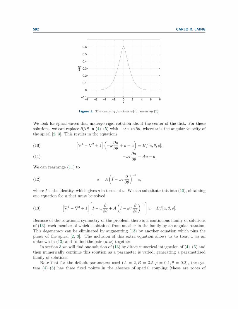
where s is Euclidian distance in Fourier space, then multiplying both sides of (8) by thedenominator of F [w] and taking the inverse two-dimensional Fourier transform result in (4).The coupling function w is given by the inverse Fourier transform of (9), which is (7), and isplotted in Figure 1. See [20, 21] for more details.

The pair of equations (5)–(6) is of the same form as those studied in [11, 32], but thedomain is now assumed to be two-dimensional. The function f we use is

f [u, θ, ρ] = H(u− θ)e−ρ/(u−θ)2 ,

where H is the Heaviside step function. In the limit as ρ → 0, f(u, θ, ρ) → H(u − θ). Weconsider the domain Ω to be a circular disk of radius R and take boundary conditions

∂u

∂r

∣∣∣∣r=R

=∂3u

∂r3

∣∣∣∣∣r=R

= 0.

592 CARLO R. LAING

−8 −6 −4 −2 0 2 4 6 8−0.1

0

0.1

0.2

0.3

0.4

0.5

0.6

r

w(r

)

Figure 1. The coupling function w(r), given by (7).

We look for spiral waves that undergo rigid rotation about the center of the disk. For thesesolutions, we can replace ∂/∂t in (4)–(5) with −ω × ∂/∂θ, where ω is the angular velocity ofthe spiral [2, 3]. This results in the equations

[∇4 −∇2 + 1

] (−ω

∂u

∂θ+ u + a

)= Bf [u, θ, ρ],(10)

−ωτ∂a

∂θ= Au− a.(11)

We can rearrange (11) to

a = A

(I − ωτ

∂

∂θ

)−1

u,(12)

where I is the identity, which gives a in terms of u. We can substitute this into (10), obtainingone equation for u that must be solved:

[∇4 −∇2 + 1

] [I − ω

∂

∂θ+ A

(I − ωτ

∂

∂θ

)−1]u = Bf [u, θ, ρ].(13)

Because of the rotational symmetry of the problem, there is a continuous family of solutionsof (13), each member of which is obtained from another in the family by an angular rotation.This degeneracy can be eliminated by augmenting (13) by another equation which pins thephase of the spiral [2, 3]. The inclusion of this extra equation allows us to treat ω as anunknown in (13) and to find the pair (u, ω) together.

In section 3 we will find one solution of (13) by direct numerical integration of (4)–(5) andthen numerically continue this solution as a parameter is varied, generating a parametrizedfamily of solutions.

Note that for the default parameters used (A = 2, B = 3.5, ρ = 0.1, θ = 0.2), the sys-tem (4)–(5) has three fixed points in the absence of spatial coupling (these are roots of

SPIRAL WAVES IN NONLOCAL EQUATIONS 593

(A + 1)u = Bf(u, θ, ρ)) at u ≈ 0, 0.58 and 1. The first and third of these fixed pointsare stable foci, whereas the second one is a saddle.

One point we do not address here is the mathematical proof of the existence of spiralwave solutions of (4)–(5). Scheel [37] has recently proven the existence of spiral waves inreaction-diffusion systems on an infinite plane, while Paullet, Ermentrout, and Troy [31] provetheir existence in an oscillatory reaction-diffusion system on a disk with Neuman boundaryconditions. The obvious difficulty with trying to use results of these authors is the nonlocalnature of (4)–(5).

2.2. Stability. To find the stability of a spiral wave, we write the evolution equations (4)–(5) as

∂u

∂t= −u + B[∇4 −∇2 + I]−1f(u) − a,(14)

∂a

∂t= Au/τ − a/τ,(15)

which become

0 = ω∂u

∂θ− u + B[∇4 −∇2 + 1]−1f(u) − a,(16)

0 = ω∂a

∂θ+ Au/τ − a/τ(17)

after moving to the rotating coordinate frame. Solutions of (16)–(17) are also solutions of (12)and (13). The Jacobian of (16)–(17) at a solution u of (13) is

J(u) =

(ω ∂

∂θ − I + B[∇4 −∇2 + 1]−1Df(u) −I

AI/τ ω ∂∂θ − I/τ

),

where I is the identity and Df(u) is the Jacobian of f at u. The eigenvalues λ and eigenfunc-tions ν giving the stability of a spiral are related by

J(u)ν = λν.

Note that ν has two components, both a “u” part and an “a” part. By differentiating (16)–(17)with respect to θ, it is clear that

ν =

(∂u∂θ∂a∂θ

)

is an eigenfunction with eigenvalue zero, where u is a solution of (13) and a = A(I−ωτ ∂∂θ )

−1u.The existence of this eigenpair is a result of the rotational symmetry of the problem [2, 3].

3. Results. Here we discuss the numerical results of continuing solutions of (13). The do-main was discretized in polar coordinates, and finite-difference approximations to the deriva-tives were used. Second-order approximations were used in both the angular and radialdirections, and the results were found to be insensitive to increases in this order. Generally,

594 CARLO R. LAING

1 1.5 2 2.5 3 3.50.1

0.15

0.2

0.25

0.3

0.35

0.4

A

ω

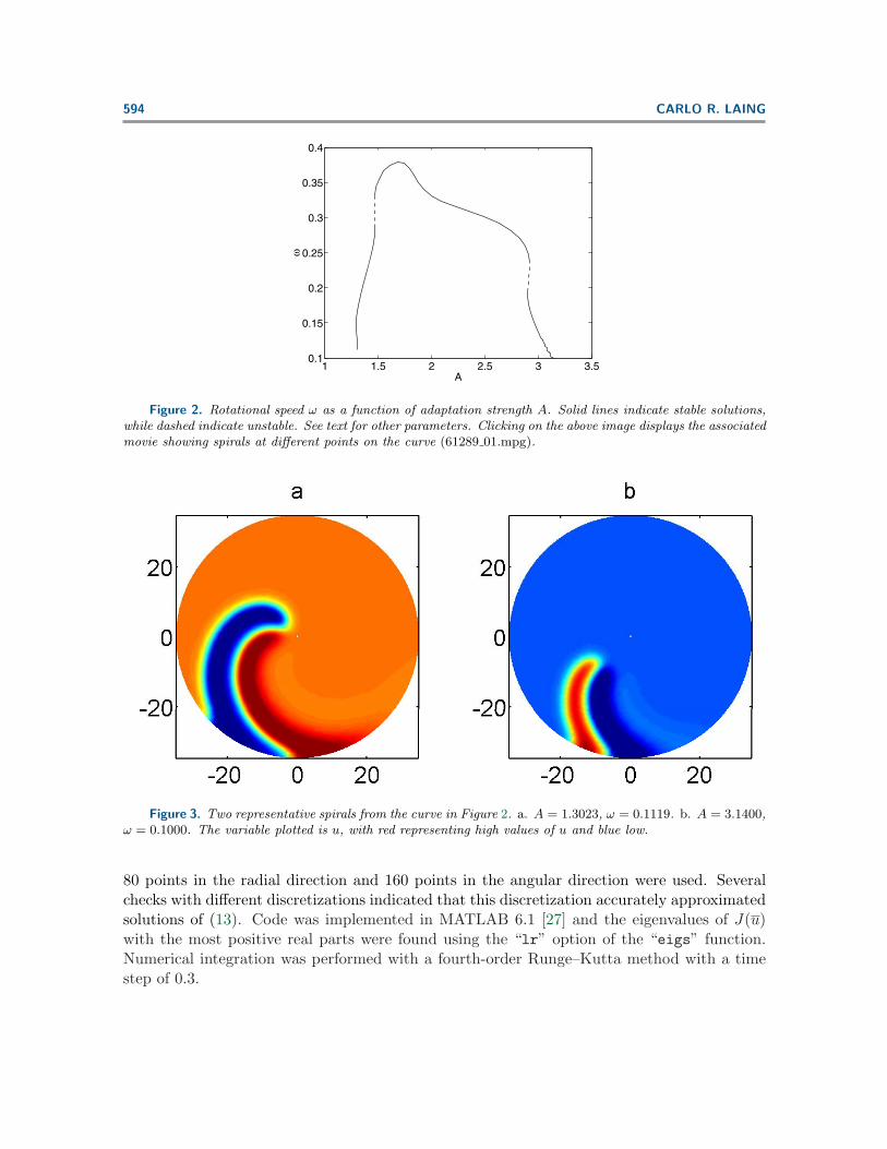
Figure 2. Rotational speed ω as a function of adaptation strength A. Solid lines indicate stable solutions,while dashed indicate unstable. See text for other parameters. Clicking on the above image displays the associatedmovie showing spirals at different points on the curve (61289 01.mpg).

Figure 3. Two representative spirals from the curve in Figure 2. a. A = 1.3023, ω = 0.1119. b. A = 3.1400,ω = 0.1000. The variable plotted is u, with red representing high values of u and blue low.

80 points in the radial direction and 160 points in the angular direction were used. Severalchecks with different discretizations indicated that this discretization accurately approximatedsolutions of (13). Code was implemented in MATLAB 6.1 [27] and the eigenvalues of J(u)with the most positive real parts were found using the “lr” option of the “eigs” function.Numerical integration was performed with a fourth-order Runge–Kutta method with a timestep of 0.3.

SPIRAL WAVES IN NONLOCAL EQUATIONS 595

−0.25 −0.2 −0.15 −0.1 −0.05 0 0.05 0.1−0.8

−0.6

−0.4

−0.2

0

0.2

0.4

0.6

Real

Imag

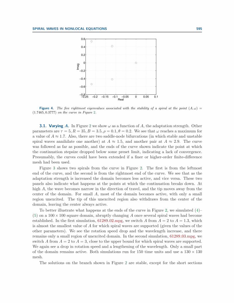
Figure 4. The five rightmost eigenvalues associated with the stability of a spiral at the point (A,ω) =(1.7465, 0.3777) on the curve in Figure 2.

3.1. Varying A. In Figure 2 we show ω as a function of A, the adaptation strength. Otherparameters are τ = 5, R = 35, B = 3.5, ρ = 0.1, θ = 0.2. We see that ω reaches a maximum fora value of A ≈ 1.7. Also, there are two saddle-node bifurcations (in which stable and unstablespiral waves annihilate one another) at A ≈ 1.5, and another pair at A ≈ 2.9. The curvewas followed as far as possible, and the ends of the curve shown indicate the point at whichthe continuation stepsize dropped below some preset limit, indicating a lack of convergence.Presumably, the curves could have been extended if a finer or higher-order finite-differencemesh had been used.

Figure 3 shows two spirals from the curve in Figure 2. The first is from the leftmostend of the curve, and the second is from the rightmost end of the curve. We see that as theadaptation strength is increased the domain becomes less active, and vice versa. These twopanels also indicate what happens at the points at which the continuation breaks down. Athigh A, the wave becomes narrow in the direction of travel, and the tip moves away from thecenter of the domain. For small A, most of the domain becomes active, with only a smallregion unexcited. The tip of this unexcited region also withdraws from the center of thedomain, leaving the center always active.

To better illustrate what happens at the ends of the curve in Figure 2, we simulated (4)–(5) on a 100× 100 square domain, abruptly changing A once several spiral waves had becomeestablished. In the first simulation, 61289 02.mpg, we switch A from A = 2 to A = 1.3, whichis almost the smallest value of A for which spiral waves are supported (given the values of theother parameters). We see the rotation speed drop and the wavelength increase, and thereremains only a small region of unexcited domain. In the second simulation, 61289 03.mpg, weswitch A from A = 2 to A = 3, close to the upper bound for which spiral waves are supported.We again see a drop in rotation speed and a lengthening of the wavelength. Only a small partof the domain remains active. Both simulations run for 150 time units and use a 130 × 130mesh.

The solutions on the branch shown in Figure 2 are stable, except for the short sections

596 CARLO R. LAING

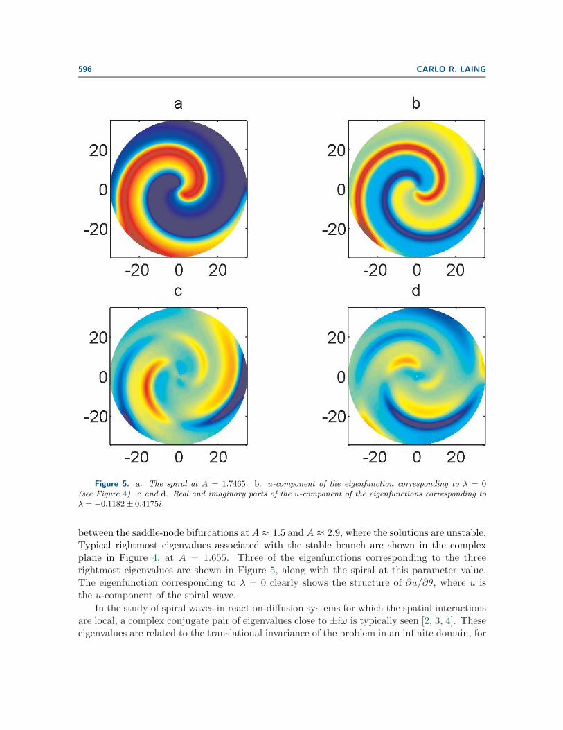
Figure 5. a. The spiral at A = 1.7465. b. u-component of the eigenfunction corresponding to λ = 0(see Figure 4). c and d. Real and imaginary parts of the u-component of the eigenfunctions corresponding toλ = −0.1182 ± 0.4175i.

between the saddle-node bifurcations at A ≈ 1.5 and A ≈ 2.9, where the solutions are unstable.Typical rightmost eigenvalues associated with the stable branch are shown in the complexplane in Figure 4, at A = 1.655. Three of the eigenfunctions corresponding to the threerightmost eigenvalues are shown in Figure 5, along with the spiral at this parameter value.The eigenfunction corresponding to λ = 0 clearly shows the structure of ∂u/∂θ, where u isthe u-component of the spiral wave.

In the study of spiral waves in reaction-diffusion systems for which the spatial interactionsare local, a complex conjugate pair of eigenvalues close to ±iω is typically seen [2, 3, 4]. Theseeigenvalues are related to the translational invariance of the problem in an infinite domain, for

SPIRAL WAVES IN NONLOCAL EQUATIONS 597

2.5 3 3.5 4 4.5 5 5.5 60.05

0.1

0.15

0.2

0.25

0.3

0.35

0.4

0.45

0.5

B

ω

Figure 6. Rotational speed ω as a function of B, the strength of the nonlinear term. Solid lines indicatestable solutions, while dashed indicate unstable. See text for other parameters. Clicking on the above imagedisplays the associated movie showing spirals at different points on the curve (61289 04.mpg).

−0.05 0 0.05 0.1 0.15 0.2 0.25 0.30.15

0.2

0.25

0.3

0.35

0.4

0.45

0.5

θ

ω

Figure 7. Rotational speed ω as a function of θ, the threshold. Solid lines indicate stable solutions, whiledashed indicate unstable. See text for other parameters. Clicking on the above image displays the associatedmovie showing spirals at different points on the curve (61289 05.mpg).

which there are eigenvalues of exactly ±iω and eigenfunctions ∂u/∂x± i∂u/∂y, where u is thespiral wave, expressed in the concentration of one of the variables. (More generally, since weare working in polar coordinates, we expect the real and imaginary parts of the eigenfunctionto be spatial derivatives of u but in orthogonal directions.) Interestingly, we do not observesuch eigenvalues in our system, with the real parts of the next rightmost eigenvalues after thezero one being −0.1182. However, the eigenfunctions corresponding to this complex conjugatepair, shown in Figure 5, do seem to have the expected structure—the real and imaginary partsare approximately the spatial derivatives of u but in orthogonal directions. This discrepancyseems likely to be due to one of two possibilities. First, the domain may be “small” relative tothe size of the spiral wave, and so the approximation of an infinite domain may be a poor one.

598 CARLO R. LAING

0.02 0.04 0.06 0.08 0.1 0.12 0.14 0.160.05

0.1

0.15

0.2

0.25

0.3

0.35

0.4

0.45

0.5

ρ

ω

Figure 8. Rotational speed ω as a function of ρ. Solid lines indicate stable solutions, while dashed indicateunstable. See text for other parameters. Clicking on the above image displays the associated movie showingspirals at different points on the curve (61289 06.mpg).

The effects of the boundaries might then be to move the eigenvalues at ±iω into the left halfplane, as has been observed in a reaction-diffusion system [2]. The second possibility is thatthere may be some intrinsic differences between nonlocal systems such as the one studied hereand reaction-diffusion systems, and these differences are the cause of the unusual eigenvaluestructure. We return to this point in section 4.

3.2. Varying B. Here we keep A = 2, with other parameters as in section 3.1, and varyB, the strength of the nonlinear term. A plot of ω as a function of B is shown in Figure 6.The behavior is very similar to that when A is varied, although increasing A corresponds todecreasing B and vice versa. There are two saddle-node bifurcations shown in Figure 6 whichseparate the curve of solutions into three branches. The upper and lower branches are stable,while the “middle” branch is unstable. Thus there is bistability over a range of values of B,for appropriate values of the other parameters. As in Figure 2, the curve was followed as faras possible, and the behavior of the spirals at either end is very similar to that discussed insection 3.1.

3.3. Varying θ. In Figure 7 we show ω as a function of θ, the threshold in the nonlinearity.We again have two saddle-node bifurcations. The middle branch, between the two bifurcations,is unstable, while the rest of the branch is stable.

3.4. Varying ρ. In Figure 8 we show ω as a function of ρ, the “steepness” of the nonlinearterm. Interestingly, we find a Hopf bifurcation along this branch. In Figure 9 we show thereal and imaginary parts of the rightmost few eigenvalues of the stability matrix as a functionof ρ. We can clearly see a complex pair of eigenvalues passing through the imaginary axisfrom left to right as ρ is decreased. From direct simulation, we find that this is a supercriticalHopf bifurcation, with a branch of quasi-periodic spirals emanating from the Hopf bifurcationas ρ is decreased. In the bottom panel of Figure 9 we also show ω, the rotational speed, as afunction of ρ. At the bifurcation, ω and the imaginary part of the eigenvalues are relatively

SPIRAL WAVES IN NONLOCAL EQUATIONS 599

0.075 0.08 0.085 0.09 0.095 0.10.25

0.3

0.35

0.4

0.45

0.5

0.55

ρ

Imag

(λ),

ω0.075 0.08 0.085 0.09 0.095 0.1

−0.1

−0.08

−0.06

−0.04

−0.02

0

0.02

0.04

ρR

eal(λ

)

Figure 9. Top: Real part of the rightmost few eigenvalues as a function of ρ along a section of the curvein Figure 8. Bottom: Imaginary part of the rightmost few eigenvalues (dotted) and ω (solid).

close; i.e., the second frequency is similar to the underlying frequency of oscillation. This ismanifested as a slow modulation of the oscillations seen in the numerical simulations to theleft of the bifurcation (not shown). This “meandering” resulting from Hopf bifurcations hasbeen observed before in reaction-diffusion systems [2, 4], and the Hopf bifurcation shown hereseems to be similar in every way to those bifurcations.

There are also two pairs of saddle-node bifurcations on the curve of solutions shown inFigure 8, and the stability is indicated in that figure.

3.5. Varying τ . A plot of ω as a function of τ is shown in Figure 10. Qualitatively, interms of the appearance of the spiral, increasing τ is similar to decreasing A and vice versa.All of the spirals on the curve in Figure 10 are stable.

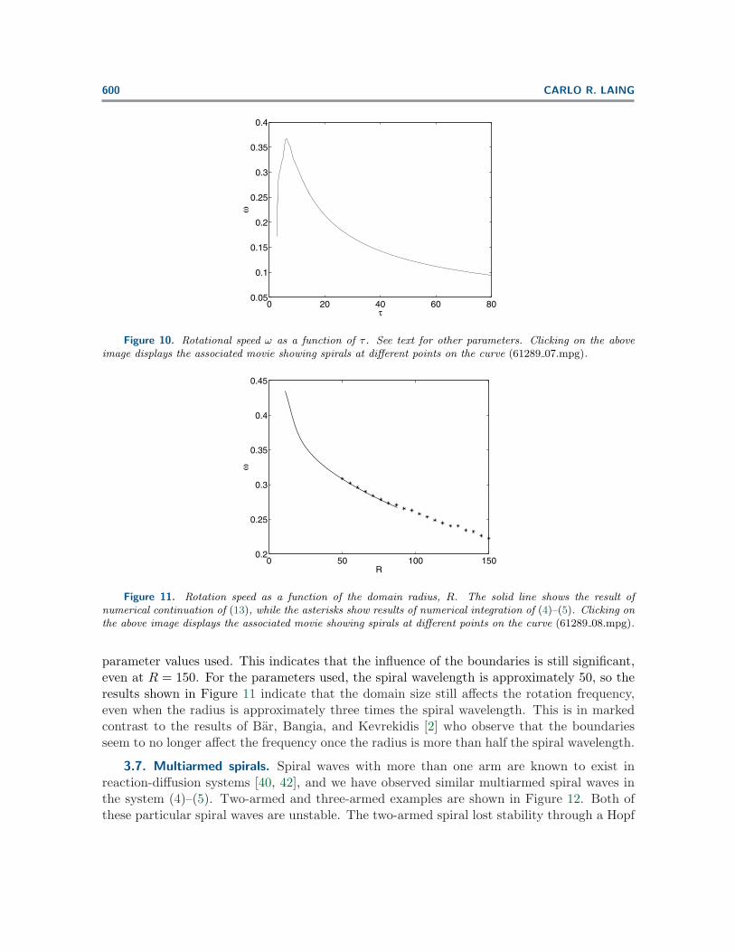
3.6. Varying R. Here we vary R, the radius of the domain. Figure 11 shows ω as afunction of R, with data from both numerical continuation of (13) and from direct simulationof (4)–(5) for large R. We see that as the domain size increases, the rotational speed drops.This type of dependence has been seen before in a reaction-diffusion system [2, 15]. All spiralson the curve shown in Figure 11 are stable, as determined by numerical integration. Thisis in contrast with the system studied by Bar, Bangia, and Kevrekidis, in which decreasingthe radius first stabilized the spiral (by moving a pair of complex eigenvalues into the lefthalf plane) and then destabilized it (the eigenvalues then moved into the right half plane).Interestingly, there is no saturation in the frequency as R is increased for the particular

600 CARLO R. LAING

0 20 40 60 800.05

0.1

0.15

0.2

0.25

0.3

0.35

0.4

τ

ω

Figure 10. Rotational speed ω as a function of τ . See text for other parameters. Clicking on the aboveimage displays the associated movie showing spirals at different points on the curve (61289 07.mpg).

0 50 100 1500.2

0.25

0.3

0.35

0.4

0.45

R

ω

Figure 11. Rotation speed as a function of the domain radius, R. The solid line shows the result ofnumerical continuation of (13), while the asterisks show results of numerical integration of (4)–(5). Clicking onthe above image displays the associated movie showing spirals at different points on the curve (61289 08.mpg).

parameter values used. This indicates that the influence of the boundaries is still significant,even at R = 150. For the parameters used, the spiral wavelength is approximately 50, so theresults shown in Figure 11 indicate that the domain size still affects the rotation frequency,even when the radius is approximately three times the spiral wavelength. This is in markedcontrast to the results of Bar, Bangia, and Kevrekidis [2] who observe that the boundariesseem to no longer affect the frequency once the radius is more than half the spiral wavelength.

3.7. Multiarmed spirals. Spiral waves with more than one arm are known to exist inreaction-diffusion systems [40, 42], and we have observed similar multiarmed spiral waves inthe system (4)–(5). Two-armed and three-armed examples are shown in Figure 12. Both ofthese particular spiral waves are unstable. The two-armed spiral lost stability through a Hopf

SPIRAL WAVES IN NONLOCAL EQUATIONS 601

Figure 12. a. A two-armed spiral. b. A three-armed spiral. u is shown color-coded. Both are unstable.Parameters are A = 2, B = 3.5, ρ = 0.1, θ = 0.2, τ = 1, R = 35.

602 CARLO R. LAING

16 18 20 22 24 26 28−0.1

−0.05

0

0.05

0.1

0.15

R

Rea

l(λ)

Figure 13. Real part of the rightmost few eigenvalues for two-armed spirals as a function of R, the domainradius. Other parameters are as in Figure 12. There is a Hopf bifurcation as R increases. Clicking on theabove image displays the associated movie of the spiral arms at R = 25 (61289 09.mpg).

bifurcation as R was increased. Figure 13 shows the real part of the rightmost few eigenvaluesassociated with this family of solutions near the bifurcation. The imaginary parts of theeigenvalues crossing the real axis are approximately ±0.55i.

The eigenfunction at this bifurcation is spatially localized at the center of the domain,so it is expected that the secondary oscillation caused by this bifurcation will appear nearthe spiral tips. This is indeed what happens, and the spiral tips start to oscillate towardand away from the center of the domain (as well as rotating around it) as R is increasedthrough R ≈ 21.5. Clicking on Figure 13 shows a movie of the evolution of a two-armedspiral at R = 25. Initially, the spirals rotate about the center of the domain, but later in thesimulation this is not the case.

The two-armed spiral is stable for small domain size, which seems to be an effect similar tothat of the boundary-induced stabilization seen by Bar, Bangia, and Kevrekidis [2]. Althoughthere is still some controversy about the instability of multiarmed spirals, the instability weobserve for a moderate-sized domain is in general agreement with observations by others inreaction-diffusion systems [13, 42].

In Figures 2, 6, 7, and 8, showing the ranges over which stable spiral waves exist, thereare upper and lower limits to those ranges. For all parameters investigated, similar behavioris seen once the system is pushed past those limits. Decreasing A, increasing B, or decreasingθ or ρ causes the whole domain to become active. Spiral waves are not supported, as therecovery variable (a) is not strong enough to return the activity variable (u) to a low valuefrom which it can be excited again. Similarly, increasing A, decreasing B, or increasing θ orρ causes the whole domain to become quiescent. In this case, the effects of the variable aoverpower those of the u, and sustained patterns are not possible. While all of the figures inthis paper have been generated for spiral waves on a circular domain, the upper and lowerbounds on parameters for existence mentioned above have all been checked on larger squaredomains and have been found to be correct (data not shown).

The bifurcation diagrams shown all relate to varying one parameter while keeping all

SPIRAL WAVES IN NONLOCAL EQUATIONS 603

of the others at particular default values. By varying any of these default values, differentdiagrams—perhaps qualitatively different ones—may be found, so we have by no means com-pletely understood the system under study. Another possible step in the study of this modelwould be to follow the codimension-one saddle-node or Hopf bifurcations in two parameters.This would help in determining regions of parameter space in which the system was bistable,for example, and might reveal higher-codimension bifurcations which could have interestingbehavior associated with them.

Although we have considered only spiral waves that rotate about the origin of the domain,which we can analyze, the system (4)–(5) is also capable of supporting spiral waves that donot rotate about the origin and the simultaneous existence of more than one of these waves,phenomena that have been observed previously [28, 30]. Spiral waves are generic phenomena,and the system studied is quite robust. We have successfully simulated spiral waves in domainswith inhomogeneities, e.g., domains for which the value of θ at each grid point is chosen froma normal distribution (not shown).

We have also observed target patterns, formed by outwardly moving concentric rings ofactive neurons. These are commonly observed in systems which also support spiral waves [16]and have been seen in simulations of large networks of spiking neurons [19]. In order for thesewaves to continue to be emitted from the center of the domain, some inhomogeneity mustbe present there. We created this inhomogeneity by decreasing the threshold, θ, in a smallcircular neighborhood of the origin. We have also observed plane waves in the absence ofinhomogeneities in the domain.

4. Conclusion. In this paper we have numerically demonstrated the existence of spiralwaves in a spatially nonlocal integro-differential equation of the form commonly used to modeltwo-dimensional neural fields. For this model, we investigated the dependence of spiral waveson the parameters of that system. We have determined the ranges of those parameters overwhich stable spirals exist. This information could be used in two different ways. If spiralwaves are viewed as undesirable (in the same way as in cardiac systems [5, 12]), we canuse this information to determine how sensitive the system is to a change in a particularparameter, by knowing how wide the parameter range is in which stable spirals exist. Wecan also determine the necessary change in a particular parameter to make the system nolonger capable of supporting a stable spiral wave. Conversely, if spiral waves are desirable, wecould use this information to steer the system toward a region in parameter space far fromany bifurcations, thus making it robust to perturbations in those parameters. Of course, forthis to be useful in a particular system we would need to know the relationships betweenthe manipulable parameters in the system and the parameters of the model we are studying.However, this study does provide the first understanding of the dependence of spiral waves inthese systems on generic parameters such as strength and timescale of the recovery variable.This model could also be used to study the general problem of the destruction of spiral wavesby applying appropriate transient stimuli instead of changing bulk parameters of the system.

We have also found two supercritical Hopf bifurcations of spirals, one that occurs for asingle-armed spiral as ρ is decreased, and one for a two-armed spiral as R is increased. Theseseem very similar to Hopf bifurcations found in reaction-diffusion systems [2, 3]. We have notinvestigated these in any depth, but it would be interesting to see what happens to the quasi-

604 CARLO R. LAING

periodic patterns created in these bifurcations as parameters are changed. We also observedmultiarmed spirals which are unstable for moderate domain sizes, in agreement with resultsobserved in reaction-diffusion systems.

Most of the results we have seen are not dissimilar to those observed in reaction-diffusionsystems with local interactions. However, the issue of the influence of domain size seems tobe unresolved. In section 3.1 we saw that the complex conjugate pair of eigenvalues of theJacobian with the most positive real part were well away from the imaginary axis, in contrastto the situation for reaction-diffusion systems [2, 3]. This may indicate that even for thisdomain size, the boundaries are affecting the stability of the spiral wave. In Figure 11 weshowed the rotation speed as a function of domain size and observed no saturation even whenthe radius was approximately three times the wavelength, indicating that even for such alarge domain, the effects of the boundary were being felt. Unfortunately, due to numericallimitations we could not reliably trace the eigenvalues of the Jacobian as the domain size wasincreased.

Regarding possible extensions of the work presented here, one interesting feature to includein the type of model we have presented would be the effects of propagation delays [7]. Althoughincluding these in models in one spatial dimension does not seem to change the stability oftravelling waves, this does not seem to carry over to two spatial dimensions [6]. Anotherfeature to include is the presence of inhibitory neurons, which also have spatially extendedcoupling [9].

There exist many results relating to spiral waves in reaction-diffusion systems; these in-clude their response to temporally periodic forcing [24, 25] or anisotropies of the domain [36],their motion near boundaries [38], the effects of differently shaped domains [43], and the in-teraction between two or more spirals [1]. A large open issue is to determine whether ornot generic behavior of spiral waves in reaction-diffusion systems also occurs in systems withnonlocal spatial interactions. Our work suggests that in at least one aspect it does not.

Acknowledgment. I thank the referees for their useful comments, which I feel have im-proved the paper.

REFERENCES

[1] I. S. Aranson, L. Kramer, and A. Weber, Theory of interaction and bound states of spiral waves inoscillatory media, Phys. Rev. E, 47 (1993), pp. 3231–3241.

[2] M. Bar, A. K. Bangia, and I. G. Kevrekidis, Bifurcation and stability analysis of rotating chemicalspirals in circular domains: Boundary-induced meandering and stabilization, Phys. Rev. E (3), 67(2003), 056126.

[3] D. Barkley, Linear stability analysis of rotating spiral waves in excitable media, Phys. Rev. Lett., 68(1992), pp. 2090–2093.

[4] D. Barkley, Euclidian symmetry and the dynamics of rotating spiral waves, Phys. Rev. Lett., 72 (1994),pp. 164–167.

[5] V. N. Biktashev, A. V. Holden, S. F. Mironov, A. M. Pertsov, and A. V. Zaitsev, Three dimen-sional aspects of re-entry in experimental and numerical models of ventricular fibrillation, Internat.J. Bifur. Chaos Appl. Sci. Engrg., 9 (1999), pp. 694–704.

[6] S. Coombes, Personal communication, 2004.[7] S. Coombes, G. J. Lord, and M. R. Owen, Waves and bumps in neuronal networks with axo-dendritic

synaptic interactions, Phys. D, 178 (2003), pp. 219–241.

SPIRAL WAVES IN NONLOCAL EQUATIONS 605

[8] M. A. Dahlem and S. C. Muller, Self-induced splitting of spiral-shaped spreading depression waves inchicken retina, Exp. Brain Res., 115 (1997), pp. 319–324.

[9] B. Ermentrout, Neural networks as spatio-temporal pattern-forming systems, Rep. Progr. Phys., 61(1998), pp. 353–430.

[10] C. Fohlmeister, W. Gerstner, R. Ritz, and J. L. van Hemmen, Spontaneous excitations in thevisual cortex: Stripes, spirals, rings, and collective bursts, Neural Comput., 7 (1995), pp. 905–914.

[11] S. E. Folias and P. C. Bressloff, Breathing pulses in an excitatory neural network, SIAM J. Appl.Dyn. Syst., 3 (2004), pp. 378–407.

[12] L. Glass and M. C. Mackey, From Clocks to Chaos: The Rhythms of Life, Princeton University Press,Princeton, NJ, 1988.

[13] V. Hakim and A. Karma, Theory of spiral wave dynamics in weakly excitable media: Asymptoticreduction to a kinematic model and applications, Phys. Rev. E (3), 60 (1999), pp. 5073–5105.

[14] M. E. Harris-White, S. A. Zanotti, S. A. Frautschy, and A. C. Charles, Spiral intercellularcalcium waves in hippocampal slice cultures, J. Neurophysiol., 79 (1998), pp. 1045–1052.

[15] N. Hartmann, M. Bar, I. G. Kevrekedis, K. Krischer, and R. Imbihl, Rotating chemical waves insmall circular domains, Phys. Rev. Lett., 76 (1996), pp. 1384–1387.

[16] M. Hendrey, K. Nam, P. Guzdar, and E. Ott, Target waves in the complex Ginzburg-Landau equation,Phys. Rev. E (3), 62 (2000), pp. 7627–7631.

[17] D. Horn and I. Opher, Solitary waves of integrate-and-fire neural models, Neural Comput., 9 (1997),pp. 1677–1690.

[18] J. Keener and J. Sneyd, Mathematical Physiology, Springer-Verlag, New York, 1998.[19] W. M. Kistler, R. Seitz, and J. L. van Hemmen, Modeling collective excitations in cortical tissue,

Phys. D, 114 (1998), pp. 273–295.[20] C. R. Laing, W. C. Troy, B. Gutkin, and G. B. Ermentrout, Multiple bumps in a neuronal model

of working memory, SIAM J. Appl. Math., 63 (2002), pp. 62–97.[21] C. R. Laing and W. C. Troy, PDE methods for nonlocal models, SIAM J. Appl. Dyn. Syst., 2 (2003),

pp. 487–516.[22] C. R. Laing and W. C. Troy, Two-bump solutions of Amari-type models of neuronal pattern formation,

Phys. D, 178 (2003), pp. 190–218.[23] G. Li, Q. Ouyang, V. Petrov, and H. L. Swinney, Transition from simple rotating chemical spirals

to meandering and traveling spirals, Phys. Rev. Lett., 77 (1996), pp. 2105–2108.[24] A. L. Lin, M. Bertram, K. Martinez, and H. L. Swinney, Resonant phase patterns in a reaction-

diffusion system, Phys. Rev. Lett., 84 (2000), pp. 4240–4243.[25] A. L. Lin, A. Hagberg, E. Meron, and H. L. Swinney, Resonance tongues and patterns in periodically

forced reaction-diffusion systems, Phys. Rev. E (3), 69 (2004), p. 066217.[26] Y. H. Liu and X. J. Wang, Spike-frequency adaptation of a generalized leaky integrate-and-fire model

neuron, J. Comput. Neurosci., 10 (2001), pp. 25–45.[27] The MathWorks, MATLAB, Natick, MA.[28] U. Middya and D. Luss, Impact of global interaction on pattern formation on a disk, J. Chem. Phys.,

102 (1995), pp. 5029–5036.[29] J. Milton and P. Jung, eds., Epilepsy as a Dynamical Disease, Springer-Verlag, New York, 2003.[30] J. D. Murray, Mathematical Biology II: Spatial Models and Biomedical Applications, 3rd ed., Springer-

Verlag, Berlin, 2003.[31] J. Paullet, B. Ermentrout, and W. Troy, The existence of spiral waves in an oscillatory reaction-

diffusion system, SIAM J. Appl. Math., 54 (1994), pp. 1386–1401.[32] D. J. Pinto and G. B. Ermentrout, Spatially structured activity in synaptically coupled neuronal

networks: I. Traveling fronts and pulses, SIAM J. Appl. Math., 62 (2001), pp. 206–225.[33] D. J. Pinto and G. B. Ermentrout, Spatially structured activity in synaptically coupled neuronal

networks: II. Lateral inhibition and standing pulses, SIAM J. Appl. Math., 62 (2001), pp. 226–243.[34] J. C. Prechtl, L. B. Cohen, B. Pesaran, P. P. Mitra, and D. Kleinfeld, Visual stimuli induce

waves of electrical activity in turtle cortex, Proc. Natl. Acad. Sci. USA, 94 (1997), pp. 7621–7626.[35] B. J. Roth, Frequency locking of meandering spiral waves in cardiac tissue, Phys. Rev. E (3), 57 (1998),

pp. 3735–3738.[36] B. J. Roth, Meandering of spiral waves in anisotropic cardiac tissue, Phys. D, 150 (2001), pp. 127–136.

606 CARLO R. LAING

[37] A. Scheel, Bifurcation to spiral waves in reaction-diffusion systems, SIAM J. Math. Anal., 29 (1998),pp. 1399–1418.

[38] J. A. Sepulchre and A. Babloyantz, Motions of spiral waves in oscillatory media and in the presenceof obstacles, Phys. Rev. E, 48 (1993), pp. 187–195.

[39] P. Tass, Oscillatory cortical activity during visual hallucinations, J. Biol. Phys., 23 (1997), pp. 21–66.[40] B. Vasiev, F. Siegert, and C. Weijer, Multiarmed spirals in excitable media, Phys. Rev. Lett., 78

(1997), pp. 2489–2492.[41] A. Winfree, Are cardiac waves relevant to epileptic wave propagation?, in Epilepsy as a Dynamical

Disease, J. Milton and P. Jung, eds., Springer-Verlag, New York, 2003.[42] R. M. Zaritski and A. M. Pertsov, Stable spiral structures and their interaction in two-dimensional

excitable media, Phys. Rev. E (3), 66 (2002), 066120.[43] V. S. Zykov and H. Engel, Dynamics of spiral waves under global feedback in excitable domains of

different shapes, Phys. Rev. E (3), 70 (2004), 016201.[44] V. S. Zykov, A. S. Mikhailov, and S. C. Muller, Controlling spiral waves in confined geometries by

global feedback, Phys. Rev. Lett., 78 (1997), pp. 3398–3401.