Speeding Up Algorithms for Hidden Markov Models by Exploiting

Repetitions

Yuri Lifshits (Caltech)

Shay Mozes (Brown Uni.)

Oren Weimann (MIT)

Michal Ziv-Ukelson (Ben-Gurion Uni.)

Hidden Markov Models (HMMs)

Transition probabilities: the probability of the weather given the previous day's weather. Pi←j = the probability to make a

transition to state i from state j

Sunny Rainy Cloudy

Hidden States : sunny, rainy, cloudy. q1 , … , qk

Emission probabilities : the probability of observing a particular observable state given that we are in a particular hidden state.

ei(σ) = the probability to observe σєΣ

given that the state is i

Observable states : the states of the process that are `visible‘

Σ ={soggy, damp, dryish, dry}

Humidity in IBM

Hidden Markov Models (HMMs)

Shortly:

• Hidden Markov Models are extensively used to model processes in many fields (error-correction, speech recognition, computational linguistics, bioinformatics)

• We show how to exploit repetitions to obtain speedup of HMM algorithms

• Can use different compression schemes

• Applies to several decoding and training algorithms

HMM Decoding and Training

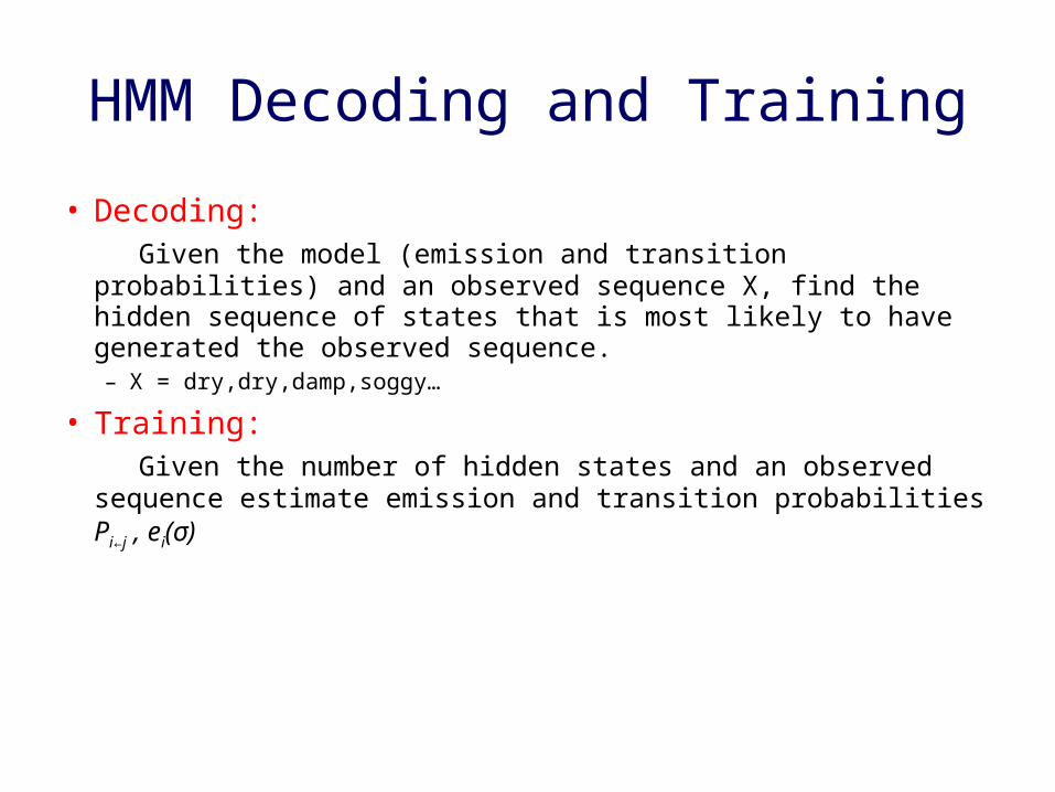
• Decoding: Given the model (emission and transition probabilities) and an

observed sequence X, find the hidden sequence of states that is most likely to have generated the observed sequence.– X = dry,dry,damp,soggy…

• Training: Given the number of hidden states and an observed sequence

estimate emission and transition probabilities Pi←j , ei(σ)

1

k

2

k

1

2

1

k

time

states

observed string

2

k

1

2

x1 x2xnx3

Decoding

• Decoding: Given the model and the observed string find the hidden sequence of states that is most likely to have generated the observed string

probability of best sequence of states that emits first 5 chars and ends in state 2

v6[4]= e4(c)·P4←2·v5[2]

probability of best sequence of states that emits first 5 chars and ends in state j

v6[4]= P4←2·v5[2]v6[4]= v5[2]v6[4]=maxj{e4(c)·P4←j·v5[j]}v5[2]

Decoding – Viterbi’s Algorithm (VA)

1 2 3 4 5 6 7 8 9 n

1

2

3

4

5

6

a a c g a c g g t

states

time

Outline

• Overview

• Exploiting repetitions

• Using Four-Russions speedup

• Using LZ78

• Using Run-Length Encoding

• Training

• Summary of results

vn=M(xn) ⊗M(xn-1) ⊗ ··· ⊗M(x1) ⊗ v0v2 = M(x2) ⊗M(x1) ⊗ v0

VA in Matrix Notation

Viterbi’s algorithm:

v1[i]=maxj{ei(x1)·Pi←j · v0[j]}

v1[i]=maxj{Mij(x1) · v0[j]}

Mij(σ) = ei (σ)·Pi←j

v1 = M(x1) ⊗ v0

(A⊗B)ij= maxk{Aik ·Bkj}

O(k2n)

O(k3n)

2

k

1

2

k

1

σ

j i

2

k

1

2

k

1

j k1

2

k

i

x1 x2

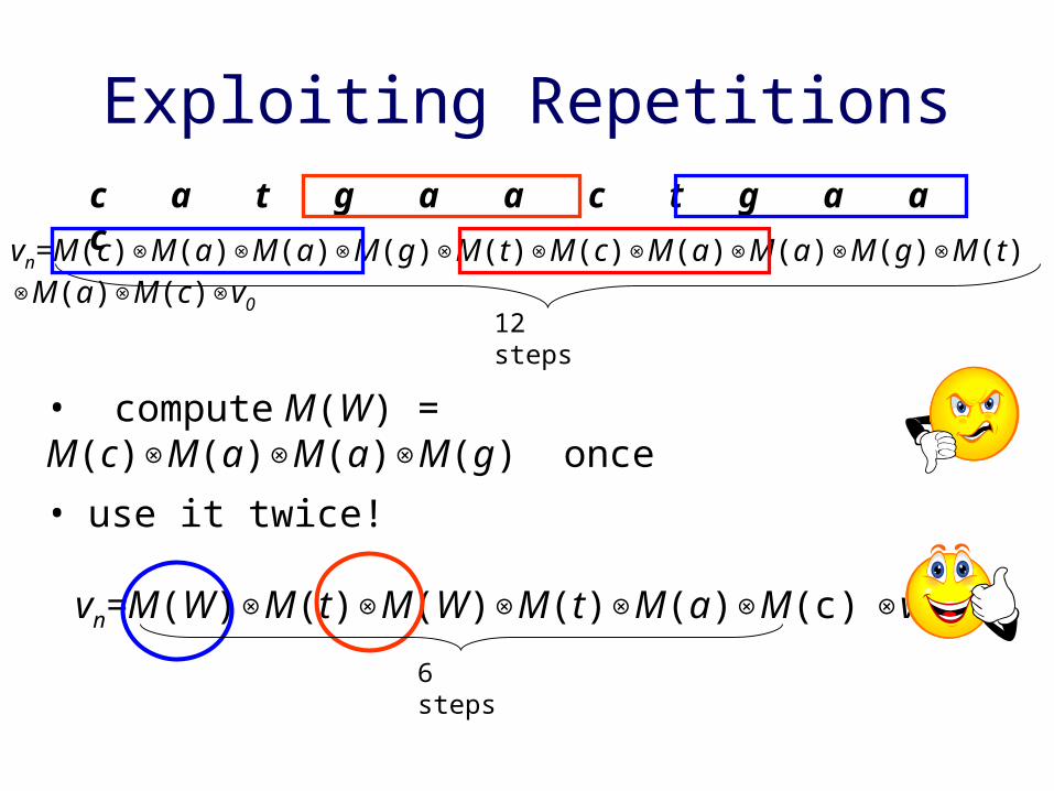
• use it twice!

vn=M(W)⊗M(t)⊗M(W)⊗M(t)⊗M(a)⊗M(c) ⊗v0

Exploiting Repetitionsc a t g a a c t g a a c

12 steps

6 steps

vn=M(c)⊗M(a)⊗M(a)⊗M(g)⊗M(t)⊗M(c)⊗M(a)⊗M(a)⊗M(g)⊗M(t)⊗M(a)⊗M(c)⊗v0

• compute M(W) = M(c)⊗M(a)⊗M(a)⊗M(g) once

ℓ - length of repetition W

λ – number of times W repeats in string

computing M(W) costs (ℓ -1)k3

each time W appears we save (ℓ -1)k2

W is good if λ(ℓ -1)k2 > (ℓ -1)k3

number of repeats = λ > k = number of states

Exploiting repetitions

>

matrix-matrix multiplication

matrix-vector multiplication

I. dictionary selection:choose the set D={Wi } of good substrings

II. encoding:compute M(Wi ) for every Wi in D

III. parsing:partition the input X into good substringsX’ = Wi1

Wi2 … Win’

IV. propagation:run Viterbi’s Algorithm on X’ using M(Wi)

General Scheme

Offline

Outline

• Overview

• Exploiting repetitions

• Using Four-Russions speedup

• Using LZ78

• Using Run-Length Encoding

• Training

• Summary of results

I. O(1)

II. O(2|Σ|l k3)

III. O(n)

IV. O(k2n / l)

Using the Four-Russians MethodCost

I. dictionary selection: D = all strings over Σ of length < l

II. encoding: incremental constructionM(Wσ)= M(W) ⊗ M(σ)

III. parsing:X’ = split X to words of length l

IV. propagation:run VA on X’ using M(Wi )

Speedup: k2n

O(2|Σ|l k3 + k2n / l)

= Θ(log n)

Outline

• Overview

• Exploiting repetitions

• Using Four-Russions speedup

• Using LZ78

• Using Run-Length Encoding

• Training

• Summary of results

Lempel Ziv 78

• The next LZ-word is the longest LZ-word previously seen plus one character

• Use a triea

c

g

g

aacgacg

• Number of LZ-words is asymptotically < n ∕ log n

I. O(n)

II. O(k3n ∕ log n)

III. O(n)

IV. O(k2n ∕ log n)

Using LZ78Cost

I. dictionary selection:D = all LZ-words in X

II. encoding: use incremental nature of LZM(Wσ)= M(W) ⊗ M(σ)

III. parsing:X’ = LZ parse of X

IV. propagation:run VA on X’ using M(Wi )

Speedup: k2n log n

k3n ∕ log n k

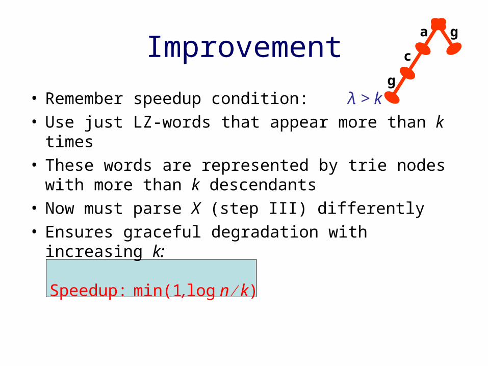
• Remember speedup condition: λ > k • Use just LZ-words that appear more than k times• These words are represented by trie nodes with more

than k descendants• Now must parse X (step III) differently• Ensures graceful degradation with increasing k:

Speedup: min(1,log n ∕ k)

Improvementa

c

g

g

Experimental Results – CpG Islands

• Short - 1.5Mbp chromosome 4 of S. Cerevisiae (yeast)• Long - 22Mbp human Y-chromosome

~x5 faster:

Outline

• Overview

• Exploiting repetitions

• Using Four-Russions speedup

• Using LZ78

• Using Run-Length Encoding

• Training

• Summary of results

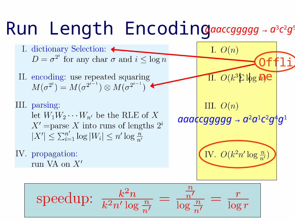
Run Length Encoding aaaccggggg → a3c2g5

aaaccggggg → a2a1c2g4g1

| |

Offline

Path traceback

• In VA, easy to do in O(n) time by keeping track of maximizing states during computation

• The problem: we only get the states on the boundaries of good substrings of X

• Solution: keep track of maximizing states when computing the matrices M(W)=M(W1) ⊗ M(W2). Takes O(n) time and O(n’k2) space

Outline

• Overview

• Exploiting repetitions

• Using Four-Russions speedup

• Using LZ78

• Using Run-Length Encoding

• Training

• Summary of results

Training

• Estimate model θ = {Pi←j , ei(σ)} given X.

– find θ that maximize P(X | θ).

• Use Expectation Maximization:1. Decoding using current θ

2. Use decoding result to update θ

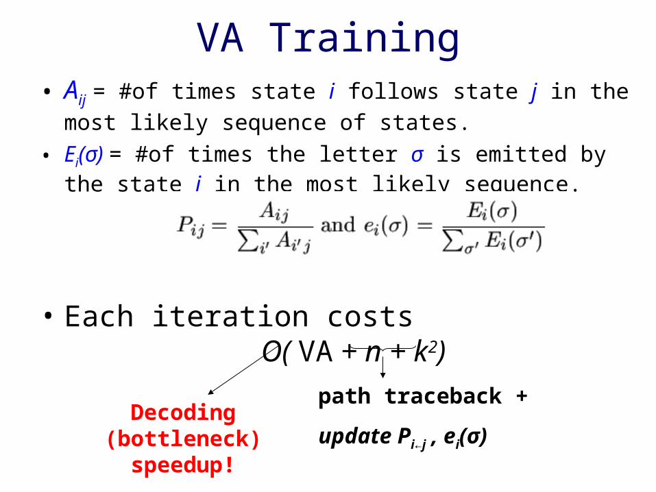
VA Training• Aij = #of times state i follows state j in the most likely

sequence of states.

• Ei(σ) = #of times the letter σ is emitted by the state i in the most likely sequence.

• Each iteration costs O( VA + n + k2)

Decoding (bottleneck) speedup!

path traceback +

update Pi←j , ei(σ)

The Forward-Backward Algorithm

– The forward algorithm calculates ft[i] the probability to observe the sequence x1, x2, …, xt requiring that the t’th state is i.

– The backward algorithm calculates bt[i] the probability to observe the sequence xt+1, xt+2, …, xn given that the t’th state is i.

ft=M(xt) ● M(xt-1) ● … ● M(x1) ● f0

bt= bn ● M(xn) ● M(xn-1) ● … ● M(xt+2) ● M(xt+1)

Baum Welch Training (in a nutshell)

• Aij = ft [j] ● Pi←j ● ei(xt+1) ● bt+1[i]

• each iteration costs: O( FB + nk2)

• If substring W has length l and repeats λ times satisfies:

then can speed up the entire process by precalculation

2

2

kl

lk

path traceback +

update Pi←j , ei(σ)

Decoding O(nk2)

Σ t

Outline

• Overview

• Exploiting repetitions

• Using Four-Russions speedup

• Using LZ78

• Using Run-Length Encoding

• Training

• Summary of results

Summary of results

• General framework • Four-Russians log(n) • LZ78 log(n) ∕ k• RLE r ∕ log(r)• Byte-Pair Encoding r• SLP, LZ77 r/k• Path reconstruction O(n)• Forward-Backward same speedups• Viterbi training same speedups• Baum-Welch training speedup, many details• Parallelization

Thank you!