speculative retail trading and asset prices published.pdf · (e.g., kumar and lee (2006), barber,...
TRANSCRIPT

JOURNAL OF FINANCIAL AND QUANTITATIVE ANALYSIS Vol. 48, No. 2, Apr. 2013, pp. 377–404COPYRIGHT 2013, MICHAEL G. FOSTER SCHOOL OF BUSINESS, UNIVERSITY OF WASHINGTON, SEATTLE, WA 98195doi:10.1017/S0022109013000100
Speculative Retail Trading and Asset Prices
Bing Han and Alok Kumar∗
Abstract
This paper examines the characteristics and pricing of stocks that are actively traded byspeculative retail investors. We find that stocks with high retail trading proportion (RTP)have strong lottery features and they attract retail investors with strong gambling propen-sity. Furthermore, these stocks tend to be overpriced and earn significantly negative alpha.The average monthly return differential between the extreme RTP quintiles is −0.60%.This negative RTP premium is stronger among stocks that have lottery features or arelocated in regions where people exhibit stronger gambling propensity. Collectively, theseresults indicate that speculative retail trading affects stock prices.
I. Introduction
Speculative trading is one of the hallmarks of financial markets. Recent stud-ies in behavioral finance indicate that certain investors, especially some retail in-vestors, are drawn toward stocks with speculative features such as high skewnessand high volatility (e.g., Kumar (2009), Dorn and Huberman (2010)). In a searchfor extreme returns, speculators may be willing to undertake large amounts ofshort-term risk even if those investments yield lower average returns. Such be-havior stands in clear contrast to the implications of traditional models of risk andreturn. However, it is consistent with some investors’ desire to gamble or prefer-ence for skewness (e.g., Shefrin and Statman (2000), Barberis and Huang (2008)),to seek sensation or entertainment in trading (e.g., Grinblatt and Keloharju (2009),Dorn and Sengmueller (2009)).
∗Han, [email protected], Rotman School of Management, University of Toronto, 105St. George St, Toronto, ON M5S 3E6, Canada, and University of Texas at Austin; Kumar, [email protected], School of Business Administration, University of Miami, 514 Jenkins Building, CoralGables, FL 33124. We thank Aydogan Alti, Nick Barberis, Robert Battalio, Hendrik Bessembinder(the editor), Keith Brown, Fangjian Fu, Rick Green, John Griffin, Jay Hartzell, Jennifer Huang,Soeren Hvidkjaer (the referee), Narasimhan Jegadeesh, Danling Jiang, Paul Koch, George Korniotis,Francisco Perez-Gonzalez, Stefan Ruenzi, Hersh Shefrin, Sophie Shive, Clemens Sialm, SheridanTitman, Masahiro Watanabe, Mark Weinstein, Joe Zhang, and seminar participants at Universityof Texas at Austin, Texas Tech University, 2008 Southwind Finance Conference at the Universityof Kansas, the 2008 Texas Finance Festival, University of Texas at Dallas, and the 2008 SingaporeInternational Conference on Finance for helpful comments and valuable suggestions. We thank JeremyPage for excellent research assistance. We also thank Brad Barber, Sudheer Chava, Paul Koch,Terrance Odean, and Amiyatosh Purnanandam for providing some of the data used in the paper. Weare responsible for all remaining errors and omissions.
377
378 Journal of Financial and Quantitative Analysis
Speculative stocks would also attract investors who derive extra nonwealthutility from the act of realizing gains. Barberis and Xiong (2012) present a modelin which investors with realization utility exhibit risk-seeking behavior. Theseinvestors may hold and trade more frequently high-volatility stocks because thosestocks offer a greater chance of realizing gains.
Motivated by these earlier studies, we examine whether speculative tradingactivities of retail investors affect asset prices. In the first part of the paper, weshow that the set of stocks in which speculation-induced trading levels are highcan be successfully characterized by the retail trading proportion (RTP) measure.The RTP of a stock is defined as the monthly dollar value of the buy- and sell-initiated small trades (trade size below $5,000) divided by the dollar value of itstotal trading volume in the same month. The small-trades data are obtained fromthe Institute for the Study of Security Markets (ISSM) and Trade and Quote (TAQ)data sets, where small trades are used as a proxy for retail trades. Our trading-based measure of retail habitat is motivated by the observation that investorsbuy and sell the stocks within their habitat more frequently. By comparing theRTP variable with actual retail holdings and trading data from a discount broker-age house, we demonstrate that RTP closely captures the preferences and tradingactivities of retail investors.
Cross-sectional analysis reveals that speculative stock attributes are impor-tant determinants of the level of retail trading in a stock. In particular, stocks withhigh idiosyncratic volatility (IVOL) and skewness or lower prices are predom-inately held and actively traded by retail investors, while institutional investorsunderweight those stocks. We also find that the characteristics of the retail clien-teles of high-RTP stocks are very similar to the characteristics of investors who ex-hibit greater propensity to speculate and gamble as documented in Kumar (2009).Furthermore, the RTP is significantly higher for firms that are headquartered inregions in which people exhibit a greater propensity to gamble. Collectively, theseresults indicate that retail speculation is an important driver of trading in high-RTPstocks.
In additional tests, we find that high levels of retail trading are at least par-tially related to the activities of investors who derive an additional positive non-wealth utility from the act of realizing gains. Specifically, consistent with theprediction of the realization utility model of Barberis and Xiong (2012), we showthat investors’ propensity to realize gains is stronger among high-volatility stocks.In addition, we demonstrate that a significant positive relation exists between theproportion of retail trading in a stock and investors’ propensity to realize gains.
Taken together, these results from the 1st part of our paper indicate that RTPcaptures speculative retail trading. High-RTP stocks have strong lottery features.They are the preferred habitat of retail investors who exhibit a stronger propensityto gamble and risk-seeking investors who derive an extra nonwealth utility whenthey realize gains.
In the 2nd part of the paper, we examine asset pricing implications of spec-ulative retail trading. We use portfolios sorted by RTP as well as the Fama-MacBeth (1973) regressions of next month’s stock returns on current RTP ofstocks. Both approaches show that high-RTP stocks have significantly lower aver-age returns. The annual, risk-adjusted RTP premium (i.e., the difference between
Han and Kumar 379
the value-weighted portfolios of the top and bottom RTP quintiles) is about−7%.This result is robust to variations in portfolio sorting and weighting methods. Itis not limited to particular sample periods. It is stronger among small stocks. Ourresults do not change materially when we follow the Asparouhova, Bessembinder,and Kalcheva (2010) method to account for the impact of potential microstructure-induced noise.
Importantly, the negative RTP premium is exclusively due to the underper-formance of high-RTP stocks and not due to the overperformance of low-RTPstocks. High-RTP stocks have a high contemporaneous return but significant neg-ative alpha the next month. Thus, high-RTP stocks tend to be overpriced. It isconsistent with the pricing impact of noise traders for high-RTP stocks, becausethese stocks not only are dominated by retail investors, they also face high lim-its to arbitrage. High-RTP stocks tend to have very low market capitalization,low price, high IVOL, low institutional ownership, and low analyst coverage(ANCOV).
Our results support several recent behavioral theories that provide reasonswhy high-RTP stocks can be overpriced. For example, Scheinkman and Xiong(2003) show that stocks are overpriced when the level of speculative trading ishigh because of the high resale option value due to large disagreement among in-vestors. Barberis and Huang (2008) show that stocks with high skewness shouldearn low average returns, because investors with cumulative prospect theory util-ity overweight tiny probabilities of large gains. Barberis and Xiong (2012) predicta low average return of stocks held and traded primarily by individual investorswho are influenced by realization utility, such as highly volatile stocks.
Results from additional tests further support that the negative RTP premiumreflects speculative retail investors’ willingness to hold and trade stocks withstrong lottery features. For example, the negative RTP premium is stronger amongstocks that have lottery features or are located in regions in which people exhibit astronger propensity to gamble.1 Furthermore, we show that the negative volatility-return relation identified in the previous literature is stronger among stocks whosetrading is dominated by retail investors.2 The pricing effects of speculative retailtrading generalize beyond the volatility-return relation. We find that lottery-typestocks (i.e., stocks with low prices, high IVOL, and high idiosyncratic skewness(ISKEW)) earn low average returns, and this negative lottery stock premium isstronger for high-RTP stocks.
Our results extend the recent literature on retail investors. In particular,Kumar (2009) examines the gambling preferences of retail investors and identi-fies investor attributes that are more strongly associated with people’s propensityto gamble. Building upon those earlier findings, we identify a proxy for retailtrading for a longer time period and use it to study the asset pricing implica-tions of speculative retail clienteles. Our asset pricing results add to the growingevidence on the importance of retail investors in the return-generating process
1Following Kumar, Page, and Spalt (2011), we use the ratio of Catholic and Protestant adherentsin a county (CPRATIO) as a proxy for people’s propensity to gamble.
2Ang, Hodrick, Xing, and Zhang (AHXZ) (2006), (2009) first documented that high-IVOL stocksearn low average returns.

380 Journal of Financial and Quantitative Analysis
(e.g., Kumar and Lee (2006), Barber, Odean, and Zhu (2009), Dorn, Huberman,and Sengmueller (2008), Hvidkjaer (2008), and Kaniel, Saar, and Titman (2008)).In broader terms, our results highlight the usefulness of a habitat-based approachfor studying asset prices.
The rest of the paper is organized as follows: In Section II, we describe ourdata sources and define the retail trading proxy RTP. In Section III, using thisproxy, we identify the stocks that speculative retail investors find attractive andverify that RTP captures speculative retail trading. In Section IV, we examine theasset pricing implications of speculative retail trading. Section V concludes thepaper.
II. Retail Trading Proxy
A. Data Sources
We use data from several sources to test our hypotheses. Our 1st main dataset contains stock-level measures of retail trading from the ISSM and the TAQdatabases for the 1983–2000 period. We use small trades (trade size ≤ $5,000)to proxy for retail trades, where like Barber et al. (2009), we use the ISSM/TAQdata only until the year 2000. The introduction of decimalized trading in 2001and order splitting by institutions due to lower trading costs imply that trade sizewould not be an effective proxy for retail trading after the year 2000. To furtherensure that the small trades reflect retail trading, we compare the ISSM/TAQ datawith the portfolio holdings and trades of a sample of individual investors from alarge U.S. discount brokerage house for the 1991–1996 period.3
We use investors’ demographic characteristics, including age, income, loca-tion (zip code), occupation, marital status, gender, etc. The demographic char-acteristics of investors in the brokerage sample are measured a few months afterthe end of the sample period (June 1997) and are provided by Infobase, Inc. Weobtain the county-level geographical variation in the religious composition acrossthe United States. We collect data on religious adherence using the “Churches andChurch Membership” files from the American Religion Data Archive. The ratio ofthe proportion of Catholics and the proportion of Protestants in a county has beenshown to be significantly related to the propensity of its residents to speculate andgamble (Kumar et al. (2011)).
We also gather data from various standard sources. The daily and monthlysplit-adjusted stock returns, stock prices, and shares outstanding for all tradedfirms are from the Center for Research on Security Prices (CRSP). Followinga common practice, we restrict the sample to firms with CRSP share codes10 and 11. Firms’ book value of equity and book value of debt are obtainedfrom Compustat. We obtain the monthly Fama-French (1993) factor returns andmonthly risk-free rates from Kenneth French’s data library.4 Both the daily and the
3See Barber and Odean (2000) for additional details about the retail investor data set and Barberet al. (2009) or Hvidkjaer (2008) for additional details about the ISSM/TAQ data sets, including theprocedure for identifying small trades.
4The data library is available at http://mba.tuck.dartmouth.edu/pages/faculty/ken.french/
Han and Kumar 381
monthly data range from Jan. 1983 to Dec. 2000. Last, we obtain stocks’ insti-tutional ownership using Thomson Reuters’ 13(f) data and analyst coverage in-formation from Thomson Reuters’ Institutional Brokers’ Estimate System (IBES)data set.
B. The RTP Measure
We compute each stock’s RTP as the ratio of the total month-t buy- and sell-initiated small-trades (trade size below $5,000) dollar volume and the total stocktrading dollar volume in the same month. We obtain the RTP measure for eachstock at the end of each month. Ideally, we would like to observe the trades of allretail investors but, unfortunately, such detailed retail trading data are not avail-able in the United States for an extended time period. Therefore, we use the buy-and sell-initiated small trades as a proxy for retail trading. Several recent studieshave used the same $5,000 trade size cutoff and adopted a similar identificationstrategy to identify retail trades (e.g., Lee and Radhakrishna (2000), Battalio andMendenhall (2005), Malmendier and Shanthikumar (2007), Barber et al. (2009),and Hvidkjaer (2008)).5
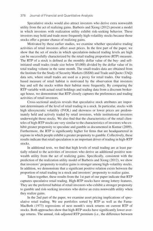
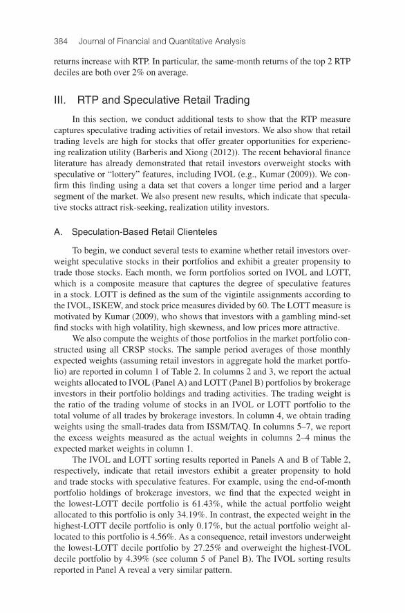
To ensure that our RTP variable reflects the behavior of retail investors, wecompare RTP with actual retail holdings and trading data from the discount bro-kerage house. Figure 1 shows the excess portfolio weight and the excess tradingweight for RTP-sorted portfolios. The excess weight reflects the difference be-tween the actual portfolio weight in the aggregate retail investors’ portfolio basedon the brokerage data and the market portfolio constructed using all CRSP stocks.The sample averages of the excess weights are shown in the figure. The excesstrading weight is defined in an analogous manner using the total trading volume(sum of buy and sell volumes) measure. Figure 1 shows that both the portfolioand trading weights in the brokerage sample increase with the level of RTP. Re-tail investors in the discount brokerage house overweight considerably and trademore stocks that have higher RTP.
In an unreported table, we estimate Fama-MacBeth (1973) and cross-sectional regressions with RTP as the dependent variable. We find that both theportfolio weight and the trading weight obtained using the actual holdings andtrades of retail investors at the discount brokerage house are strongly and posi-tively correlated with the RTP measure. Together, these findings suggest that ourRTP measure captures the preferences and trading behavior of retail investorsreasonably well.
C. Characteristics of RTP-Sorted Portfolios
To further examine the ability of the RTP measure to capture retail behaviorand to gain insights into the stock preferences of retail investors, each monthwe sort stocks into deciles based on their RTP. Table 1 reports the mean stock
5Lee and Radhakrishna (2000) show that the $5,000 trade size cutoff can effectively identify tradesinitiated by retail investors. Barber et al. (2009) report that the time-series correlations between tradingmeasures obtained using the small-trades data from ISSM/TAQ and those computed directly usingindividual investor trades at 2 different brokerage houses are high (around 0.50).

382 Journal of Financial and Quantitative Analysis
FIGURE 1
Trade Size and Retail Trading
Figure 1 shows the average portfolio and retail trading weights in the brokerage data, conditional upon the level of retailtrading proportion (RTP) of the stock. The RTP measure is defined as the ratio of the total buy- and sell-initiated small-trades(trade size below $5,000) dollar volume and the total market dollar trading volume. The small-trades data are from Institutefor the Study of Security Markets (ISSM) and Trade and Quote (TAQ) databases, where small trades are used as a proxy forretail trades. The excess weight is defined as the difference between actual and expected weights. The expected decileweight is the total weight of the decile stocks in the aggregate market portfolio. The market portfolio is defined by includingall stocks available in the CRSP database. The actual decile weight in a certain month t is defined as the month-t weightof decile stocks in the aggregate portfolio of individual investors. The aggregate individual investor portfolio is obtainedby combining the portfolios of all investors. The weights are standardized (mean is set to 0 and the standard deviation is1) to facilitate comparisons between the 2 weight measures. The averages of those weights for the Jan. 1991–Nov. 1996sample period are shown in the figure.
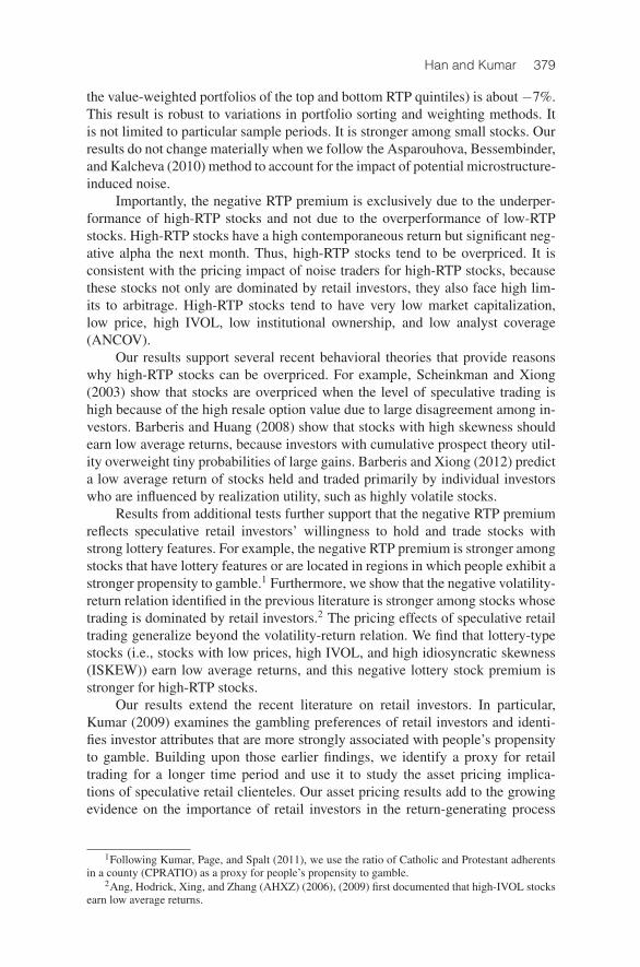
characteristics of RTP-sorted portfolios for the 1983–2000 time period. There isvery little retail trading in the bottom 5 RTP deciles. The RTP is only 0.74% onaverage for the lowest-RTP decile. Even for the 8th decile, the RTP is 20.57%.The majority of retail trading is concentrated in stocks ranked in the top 2 decilesby RTP. The RTP is 63.75% on average for the top decile.
Consistent with the idea that RTP captures retail preferences, we find that astock’s institutional ownership, market capitalization and stock price all decreasemonotonically with RTP. Stocks in the top 3 RTP deciles all have average pricebelow $10 and average market value below $100 million dollars. Together, thetop 5 RTP deciles represent less than 10% of the total stock market capitalization.The stocks in the highest-RTP decile have an average institutional ownership ofonly 3.01%, with 57.72% of stocks having IO below 5%. In contrast, the averageIO for the lowest-RTP decile is 50.78%, and only 3.19% stocks in this decile haveIO below 5%.
Although the level of IO declines monotonically across the RTP deciles, themagnitude of the correlation between RTP and IO is not very high. The averagecorrelation between RTP and 1−IO is 0.193 when we compute the cross-sectionalcorrelation each quarter and then take the average across all quarters. This corre-lation is even lower (only 0.049) when we first compute time-series correlations
Han and Kumar 383
TABLE 1
Small-Trades Volume and Stock Characteristics
Table 1 reports the mean stock characteristics of retail trading proportion (RTP) sorted decile portfolios. The RTP is definedas the ratio of the total monthly buy- and sell-initiated small-trades (trade size below $5,000) dollar volume and the totalmarket dollar trading volume during the same month. Small trades are used as a proxy for retail trades. The small-tradesdata are from Institute for the Study of Security Markets (ISSM) and Trade and Quote (TAQ) databases. The following stockcharacteristic measures are reported: idiosyncratic volatility (IVOL), idiosyncratic skewness (ISKEW), stock price, lotterystock index (LOTT), firm size (in billion dollars), book-to-market (BM) ratio, past 12-month return (12mRet), contempora-neous monthly stock return (RET), institutional ownership (IO), proportion of stocks in the portfolio with low (less than 5%)institutional ownership (Low IO), and analyst coverage (ANCOV). The IVOL in month t is defined as the standard deviationof the residual from a 4-factor model (the 3 Fama-French (1993) factors and the momentum factor), where daily returnsfrom month t are used to estimate the model. ISKEW is defined as the scaled 3rd moment of residuals from a factor modelthat contains market return over the risk-free rate (RMRF) and RMRF2 as factors. LOTT is defined as the sum of the vigintileassignments according to the IVOL, ISKEW, and stock price measures divided by 60. The “FracMkt” column reports thefraction of the market represented by the RTP decile portfolio. Each decile portfolio contains an average of 410 stocks.The sample period is Jan. 1983–Dec. 2000. The institutional holdings data are from Thomson Reuters. The salient numbersare shown in bold.
RTP Mean Size LowDecile RTP FracMkt IVOL ISKEW Price LOTT ($b) BM 12mRet RET IO IO ANCOV
Low 0.74% 39.26% 11.66% 0.386 $46.19 0.269 $3.145 0.592 31.62% 0.47% 50.78% 3.19% 11.59D2 1.66% 24.56% 12.03% 0.398 $27.16 0.296 $1.556 0.639 27.71% 0.43% 44.56% 3.23% 9.57D3 2.70% 15.59% 13.07% 0.402 $23.20 0.332 $0.956 0.675 26.14% 0.91% 38.65% 4.41% 7.29D4 4.09% 9.06% 13.89% 0.414 $19.67 0.369 $0.546 0.719 23.54% 1.03% 32.79% 6.59% 5.54D5 6.04% 5.04% 15.12% 0.437 $16.83 0.408 $0.299 0.739 20.94% 1.26% 27.74% 9.12% 4.18D6 8.86% 2.95% 16.47% 0.493 $13.98 0.453 $0.174 0.765 17.10% 1.19% 23.15% 13.09% 3.08D7 13.27% 1.76% 18.54% 0.560 $11.20 0.508 $0.103 0.785 13.13% 1.87% 18.93% 18.52% 2.14D8 20.57% 0.98% 22.20% 0.610 $8.28 0.581 $0.058 0.783 7.86% 2.04% 14.83% 26.54% 1.37D9 33.64% 0.56% 28.50% 0.678 $5.44 0.671 $0.032 0.729 1.62% 2.22% 10.92% 38.14% 0.79High 63.75% 0.24% 41.51% 0.745 $2.97 0.776 $0.014 0.871 −11.46% 2.12% 3.01% 57.72% 0.30
between RTP and 1−IO for each stock and then average the correlations over allstocks. These comparisons indicate that RTP is not merely some linear transfor-mation of 1−IO.6
Table 1 also shows that the average IVOL and ISKEW increase, while stockprice decreases monotonically across the RTP decile portfolios.7 The stocks in thehighest-RTP decile have an average IVOL of 41.51%, while those in the lowest-RTP decile have an average IVOL of only 11.66%. Similarly, the average ISKEWfor the highest-RTP decile portfolio is 0.745, which is almost twice the averageISKEW of 0.386 for the lowest-RTP decile portfolio. These estimates, along withthe monotonically increasing pattern in the lottery stock index (LOTT) column,indicate that the levels of retail trading are higher among stocks that are usuallyperceived as speculative stocks.
Examining other stock characteristics of RTP-sorted portfolios, we find thatstocks with a high fraction of retail trading have higher book-to-market (BM)ratios, lower ANCOV, and lower past returns. In fact, the highest-RTP decilestocks earn an average of−11.46% over the past 12 months, while the lowest-RTPdecile stocks earn an average of 31.62%. Furthermore, the contemporaneous stock
6See Hvidkjaer (2008) for additional comparisons between the ISSM/TAQ small-trades data andthe 13(f) institutional holdings data. The key conclusion from his analysis is also that the ISSM/TAQsmall-trades data do not merely proxy for 1−IO.
7Following AHXZ (2006), we measure a stock’s IVOL in a given month-t as the standard deviationof the residual obtained by fitting a 4-factor model Fama-French (1993) 3 factors plus a momentumfactor to its daily returns during month t. ISKEW is computed using the Harvey and Siddique (2000)method. It is defined as the scaled measure of the 3rd moment of the residual obtained by fitting a2-factor (RMRF and RMRF2) model to daily returns from the previous 6 months, where RMRF is themarket return, excess over the risk-free rate.
384 Journal of Financial and Quantitative Analysis
returns increase with RTP. In particular, the same-month returns of the top 2 RTPdeciles are both over 2% on average.
III. RTP and Speculative Retail Trading
In this section, we conduct additional tests to show that the RTP measurecaptures speculative trading activities of retail investors. We also show that retailtrading levels are high for stocks that offer greater opportunities for experienc-ing realization utility (Barberis and Xiong (2012)). The recent behavioral financeliterature has already demonstrated that retail investors overweight stocks withspeculative or “lottery” features, including IVOL (e.g., Kumar (2009)). We con-firm this finding using a data set that covers a longer time period and a largersegment of the market. We also present new results, which indicate that specula-tive stocks attract risk-seeking, realization utility investors.
A. Speculation-Based Retail Clienteles
To begin, we conduct several tests to examine whether retail investors over-weight speculative stocks in their portfolios and exhibit a greater propensity totrade those stocks. Each month, we form portfolios sorted on IVOL and LOTT,which is a composite measure that captures the degree of speculative featuresin a stock. LOTT is defined as the sum of the vigintile assignments according tothe IVOL, ISKEW, and stock price measures divided by 60. The LOTT measure ismotivated by Kumar (2009), who shows that investors with a gambling mind-setfind stocks with high volatility, high skewness, and low prices more attractive.
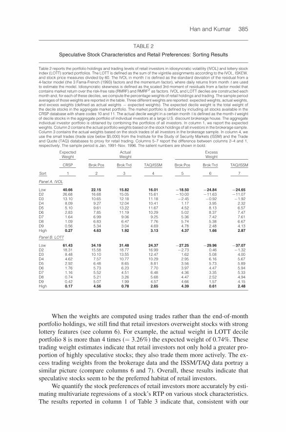
We also compute the weights of those portfolios in the market portfolio con-structed using all CRSP stocks. The sample period averages of those monthlyexpected weights (assuming retail investors in aggregate hold the market portfo-lio) are reported in column 1 of Table 2. In columns 2 and 3, we report the actualweights allocated to IVOL (Panel A) and LOTT (Panel B) portfolios by brokerageinvestors in their portfolio holdings and trading activities. The trading weight isthe ratio of the trading volume of stocks in an IVOL or LOTT portfolio to thetotal volume of all trades by brokerage investors. In column 4, we obtain tradingweights using the small-trades data from ISSM/TAQ. In columns 5–7, we reportthe excess weights measured as the actual weights in columns 2–4 minus theexpected market weights in column 1.
The IVOL and LOTT sorting results reported in Panels A and B of Table 2,respectively, indicate that retail investors exhibit a greater propensity to holdand trade stocks with speculative features. For example, using the end-of-monthportfolio holdings of brokerage investors, we find that the expected weight inthe lowest-LOTT decile portfolio is 61.43%, while the actual portfolio weightallocated to this portfolio is only 34.19%. In contrast, the expected weight in thehighest-LOTT decile portfolio is only 0.17%, but the actual portfolio weight al-located to this portfolio is 4.56%. As a consequence, retail investors underweightthe lowest-LOTT decile portfolio by 27.25% and overweight the highest-IVOLdecile portfolio by 4.39% (see column 5 of Panel B). The IVOL sorting resultsreported in Panel A reveal a very similar pattern.
Han and Kumar 385
TABLE 2
Speculative Stock Characteristics and Retail Preferences: Sorting Results
Table 2 reports the portfolio holdings and trading levels of retail investors in idiosyncratic volatility (IVOL) and lottery stockindex (LOTT) sorted portfolios. The LOTT is defined as the sum of the vigintile assignments according to the IVOL, ISKEW,and stock price measures divided by 60. The IVOL in month t is defined as the standard deviation of the residual from a4-factor model (the 3 Fama-French (1993) factors and the momentum factor), where daily returns from month t are usedto estimate the model. Idiosyncratic skewness is defined as the scaled 3rd moment of residuals from a factor model thatcontains market return over the risk-free rate (RMRF) and RMRF2 as factors. IVOL and LOTT deciles are constructed eachmonth and, for each of these deciles, we compute the percentage weights of retail holdings and trading. The sample periodaverages of those weights are reported in the table. Three different weights are reported: expected weights, actual weights,and excess weights (defined as actual weights − expected weights). The expected decile weight is the total weight ofthe decile stocks in the aggregate market portfolio. The market portfolio is defined by including all stocks available in theCRSP database with share codes 10 and 11. The actual decile weight in a certain month t is defined as the month-t weightof decile stocks in the aggregate portfolio of individual investors at a large U.S. discount brokerage house. The aggregateindividual investor portfolio is obtained by combining the portfolios of all investors. In column 1, we report the expectedweights. Column 2 contains the actual portfolio weights based on the stock holdings of all investors in the brokerage sample.Column 3 contains the actual weights based on the stock trades of all investors in the brokerage sample. In column 4, weuse the small trades (trade size below $5,000) from the Institute for the Study of Security Markets (ISSM) and the Tradeand Quote (TAQ) databases to proxy for retail trading. Columns 5–7 report the difference between columns 2–4 and 1,respectively. The sample period is Jan. 1991–Nov. 1996. The salient numbers are shown in bold.
Expected Actual ExcessWeight Weight Weight
CRSP Brok:Pos Brok:Trd TAQ/ISSM Brok:Pos Brok:Trd TAQ/ISSM
Sort 1 2 3 4 5 6 7
Panel A. IVOL
Low 40.66 22.15 15.82 16.01 −18.50 −24.84 −24.65D2 26.68 16.68 15.05 15.61 −10.00 −11.63 −11.07D3 13.10 10.65 12.18 11.18 −2.45 −0.92 −1.92D4 8.09 9.27 12.04 10.41 1.17 3.95 2.32D5 5.10 9.61 13.22 11.67 4.52 8.13 6.57D6 2.83 7.85 11.19 10.29 5.02 8.37 7.47D7 1.64 6.99 9.06 9.25 5.36 7.42 7.61D8 1.09 6.83 6.47 7.76 5.74 5.38 6.67D9 0.56 5.34 3.04 4.69 4.78 2.48 4.13High 0.27 4.63 1.92 3.13 4.37 1.66 2.87
Panel B. LOTT
Low 61.43 34.19 31.48 24.37 −27.25 −29.96 −37.07D2 18.31 15.58 18.77 16.99 −2.73 0.46 −1.32D3 8.48 10.10 13.55 12.47 1.62 5.08 4.00D4 4.62 7.57 10.77 10.29 2.95 6.16 5.67D5 2.92 6.48 8.65 8.81 3.56 5.73 5.89D6 1.76 5.73 6.23 7.70 3.97 4.47 5.94D7 1.16 5.52 4.51 6.48 4.36 3.35 5.33D8 0.74 5.21 3.26 5.68 4.47 2.52 4.94D9 0.42 5.07 1.99 4.57 4.66 1.57 4.15High 0.17 4.56 0.78 2.65 4.39 0.61 2.48
When the weights are computed using trades rather than the end-of-monthportfolio holdings, we still find that retail investors overweight stocks with stronglottery features (see column 6). For example, the actual weight in LOTT decileportfolio 8 is more than 4 times (= 3.26%) the expected weight of 0.74%. Thesetrading weight estimates indicate that retail investors not only hold a greater pro-portion of highly speculative stocks; they also trade them more actively. The ex-cess trading weights from the brokerage data and the ISSM/TAQ data portray asimilar picture (compare columns 6 and 7). Overall, these results indicate thatspeculative stocks seem to be the preferred habitat of retail investors.
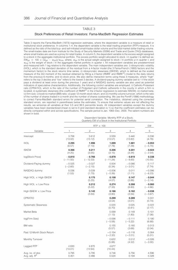
We quantify the stock preferences of retail investors more accurately by esti-mating multivariate regressions of a stock’s RTP on various stock characteristics.The results reported in column 1 of Table 3 indicate that, consistent with our
386 Journal of Financial and Quantitative Analysis
TABLE 3
Stock Preferences of Retail Investors: Fama-MacBeth Regression Estimates
Table 3 reports the Fama-MacBeth (1973) regression estimates, where the dependent variable is a measure of retail orinstitutional stock preference. In columns 1–4, the dependent variable is the retail trading proportion (RTP) measure. It isdefined as the ratio of the total buy- and sell-initiated small-trades dollar volume and the total market dollar trading volume.The small-trades data are from Institute for the Study of Security Markets (ISSM) and Trade and Quote (TAQ) databases,where small trades are used as a proxy for retail trades. In column 5, the dependent variable is the excess weight assignedto a stock in the aggregate institutional portfolio. The excess portfolio weight allocated to stock i in quarter t is defined as:EWipt = 100 × (wipt − wimt)/wimt, where, wipt is the actual weight assigned to stock i in portfolio p in quarter t, andwimt is the weight of stock i in the aggregate market portfolio in quarter t. All independent variables are predeterminedand measured with 1 lag relative to the dependent variable. The main independent variables are: i) idiosyncratic volatility(IVOL), which is the standard deviation of the residual from a 4-factor model (the 3 Fama-French (1993) factors and themomentum factor) to the stock returns time series; ii) idiosyncratic skewness (ISKEW), which is defined as the scaledmeasure of the 3rd moment of the residual obtained by fitting a 2-factor (RMRF and RMRF2) model to the daily returnsfrom the previous 6 months; and iii) stock price. We also define interaction terms using these 3 measures, where “high”refers to the top 3 deciles and “low” refers to the lowest 3 deciles. A dividend-paying dummy variable (set to 1 if the stockpays a dividend at least once during the previous 1 year) and a NASDAQ dummy variable are also used as potentialindicators of speculative characteristics. Additionally, the following control variables are employed: i) Catholic-Protestantratio (CPRATIO), which is the ratio of the number of Protestant and Catholic adherents in the county in which a firm islocated; ii) systematic skewness (the coefficient of RMRF2 in the 2-factor regression to estimate ISKEW); iii) market beta;iv) firm size; v) book-to-market (BM) ratio; vi) past 12-month stock return; and vii) monthly volume turnover, which is the ratioof the number of shares traded in a month and the number of shares outstanding. We use the Pontiff (1996) methodologyto correct Fama-MacBeth standard errors for potential serial correlation. The t-statistics, obtained using the correctedstandard errors, are reported in parentheses below the estimates. To ensure that extreme values are not affecting theresults, we winsorize all variables at their 0.5 and 99.5 percentile levels. All independent variables except the dummyvariables have been standardized (mean is set to 0 and standard deviation is 1) so that the coefficient estimates can bedirectly compared within and across specifications. The sample period is Jan. 1983–Dec. 2000. The salient numbers areshown in bold.
Dependent Variable: Monthly RTP of a Stock;Quarterly EW of a Stock in the Institutional Portfolio
RTP× 100 EW
Variable 1 2 3 4 5
Intercept 3.706 3.612 3.559 3.440 0.036(13.02) (13.12) (13.57) (13.82) (4.78)
IVOL 2.295 1.996 1.699 1.681 −0.053(8.57) (7.10) (7.78) (7.29) (−5.70)
ISKEW 0.366 0.211 0.206 0.201 −0.024(4.25) (3.55) (3.15) (3.34) (−2.54)
log(Stock Price) −0.810 −0.766 −0.878 −0.819 0.338(−11.50) (−12.33) (−11.24) (−8.60) (10.50)
Dividend-Paying dummy −0.025 −0.027 0.004 −0.066 0.117(−2.60) (−2.10) (0.34) (−3.01) (7.74)
NASDAQ dummy 0.036 0.039 −0.006 0.011 −0.096(1.53) (1.70) (−0.26) (1.11) (−6.23)
High IVOL× High ISKEW 0.175 0.158 0.147 −0.044(5.20) (4.07) (3.88) (−3.14)
High IVOL× Low Price 0.212 0.274 0.268 −0.060(5.22) (7.33) (6.80) (−4.66)
High ISKEW× Low Price 0.142 0.166 0.162 −0.038(3.50) (3.80) (3.54) (−3.67)
CPRATIO 0.299 0.289 0.031(3.54) (3.01) (0.74)
Systematic Skewness 0.020 0.025 0.022(0.70) (0.81) (2.17)
Market Beta 0.099 0.149 0.101(1.13) (1.80) (7.08)
log(Firm Size) −0.098 −0.111 0.190(−5.58) (−5.22) (6.68)
BM ratio 0.155 0.160 0.013(5.57) (3.68) (2.04)
Past 12-Month Stock Return −0.154 −0.118 0.084(−2.32) (−2.01) (5.01)
Monthly Turnover 0.622 0.512 −0.026(5.88) (4.52) (−3.00)
Lagged RTP 4.830 4.870 4.677(13.01) (12.64) (10.44)
Avg. no. of obs. 3,795 3,795 3,748 3,756 4,596Avg. adj. R2 0.451 0.486 0.524 0.194 0.328
Han and Kumar 387
univariate sorting results, all else being equal, retail investors trade stocks withhigh IVOL more actively. RTP levels are also higher for stocks that are likely tobe viewed as speculative instruments, such as stocks with low prices, high ISKEWlevels, and nondividend-paying status.
To further establish that RTP captures the speculative preferences of retail in-vestors, we introduce several interaction terms in the RTP regression specificationusing price, IVOL, and ISKEW variables. The regression estimates in column 2of Table 3 show that High IVOL × Low Price and High IVOL × High ISKEWinteraction terms have significantly positive coefficient estimates. Thus, stockswith higher IVOL have even higher RTP if they are both low priced and have highISKEW. Similarly, the significantly positive estimate of the High ISKEW × LowPrice interaction dummy variable indicates that high-skewness stocks have higherlevels of RTP if they also have low prices.
We also test whether the RTP is higher for firms located in regions in whichpeople exhibit a stronger propensity to gamble. This test is motivated by the priorevidence, which indicates that investors disproportionately hold and trade localstocks and that gambling propensities across different domains are positively cor-related. Following Kumar et al. (2011), we use the ratio of Catholic and Protestantadherents in a county (CPRATIO) as a proxy for people’s propensity to gamble.8
Using this gambling proxy, we find that the RTP levels are higher in regions with ahigher CPRATIO (see columns 3 and 4 of Table 3). This evidence further supportsour conjecture that RTP reflects the speculative behavior of retail investors.9
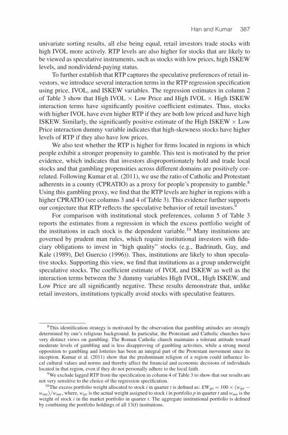
For comparison with institutional stock preferences, column 5 of Table 3reports the estimates from a regression in which the excess portfolio weight ofthe institutions in each stock is the dependent variable.10 Many institutions aregoverned by prudent man rules, which require institutional investors with fidu-ciary obligations to invest in “high quality” stocks (e.g., Badrinath, Gay, andKale (1989), Del Guercio (1996)). Thus, institutions are likely to shun specula-tive stocks. Supporting this view, we find that institutions as a group underweightspeculative stocks. The coefficient estimate of IVOL and ISKEW as well as theinteraction terms between the 3 dummy variables High IVOL, High ISKEW, andLow Price are all significantly negative. These results demonstrate that, unlikeretail investors, institutions typically avoid stocks with speculative features.
8This identification strategy is motivated by the observation that gambling attitudes are stronglydetermined by one’s religious background. In particular, the Protestant and Catholic churches havevery distinct views on gambling. The Roman Catholic church maintains a tolerant attitude towardmoderate levels of gambling and is less disapproving of gambling activities, while a strong moralopposition to gambling and lotteries has been an integral part of the Protestant movement since itsinception. Kumar et al. (2011) show that the predominant religion of a region could influence lo-cal cultural values and norms and thereby affect the financial and economic decisions of individualslocated in that region, even if they do not personally adhere to the local faith.
9We exclude lagged RTP from the specification in column 4 of Table 3 to show that our results arenot very sensitive to the choice of the regression specification.
10The excess portfolio weight allocated to stock i in quarter t is defined as: EWipt = 100× (wipt −wimt)/wimt,where, wipt is the actual weight assigned to stock i in portfolio p in quarter t and wimt is theweight of stock i in the market portfolio in quarter t. The aggregate institutional portfolio is definedby combining the portfolio holdings of all 13(f) institutions.

388 Journal of Financial and Quantitative Analysis
B. Additional Evidence of Speculative Retail Clienteles
To further test the claim that RTP captures the speculative behavior of retailinvestors, we examine the characteristics of the retail investor clientele of high-RTP stocks. We conjecture that the characteristics of retail clienteles of high-RTPstocks would be similar to the characteristics of investors who are more likelyto engage in speculative or gambling-motivated trading (e.g., younger, male, lesseducated, and low-income investors), as documented in Kumar (2009).
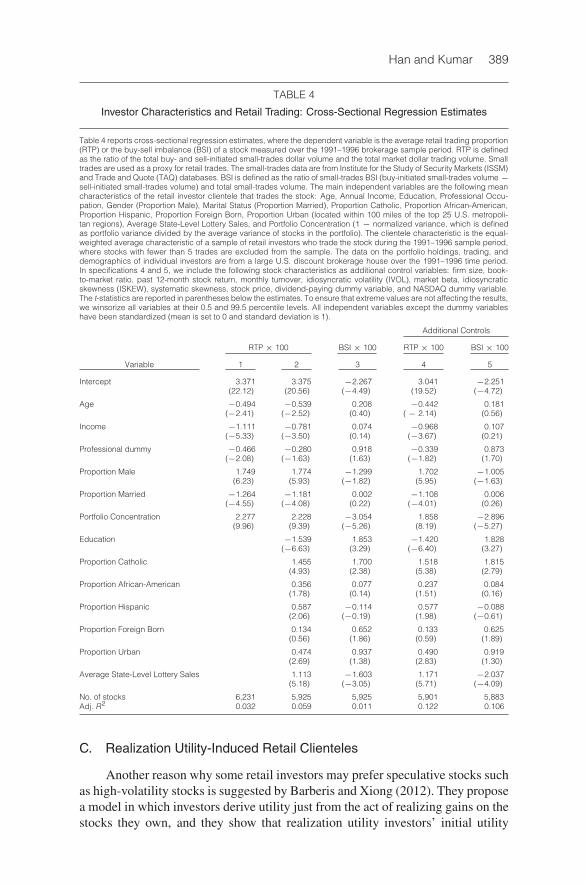
We test this hypothesis using the retail investors’ holdings from a large U.S.discount brokerage house for the 1991–1996 period and their demographic char-acteristics. For each stock, we measure the average characteristics of broker-age investors who trade the stock during the 6-year sample period. Using theseclientele characteristics, we estimate a cross-sectional regression in which thesample-period average RTP for a stock is the dependent variable, and the averageclientele characteristics of the stock are the independent variables. The results arereported in Table 4. In column 1, we report estimates from a specification thatonly includes characteristics that are available in the brokerage data, and in col-umn 2, we consider additional characteristics defined using measures associatedwith investors’ location.
We find that stocks with high levels of RTP have younger clienteles withlower income, lower education levels, and nonprofessional occupations. Thosestocks also have a greater proportion of male and single investors. Retail investorsof high-RTP stocks tend to hold less-diversified portfolios. Moreover, the RTP ishigh for stocks that are held by urban investors and those who reside in areas withhigher per capita lottery expenditures. Both of these geographical characteristicsare associated with a greater propensity to speculate and gamble. These demo-graphic characteristics, along with the religious and racial/ethnic characteristicsof high-RTP stocks, are very similar to the characteristics of investors who aremore attracted toward speculative and lottery-type stocks (Kumar (2009)). Theseresults further support that RTP is a good proxy for retail speculation.
When we consider an alternative measure of retail trading that captures thedirection of trading (i.e., the buy-sell imbalance (BSI)), we find completely dif-ferent results (see column 3 of Table 4).11 Stocks with higher levels of BSI donot have clientele characteristics that are similar to the characteristics of investorswho find speculative stocks attractive. The BSI regression estimates indicate thatRTP is a more appropriate proxy than BSI for retail speculation. This evidencealso indicates that speculative investors are not merely accumulating the shares ofthe stocks they like. Rather, they actively buy as well as sell those stocks.
For robustness, in columns 4 and 5 of Table 4, we report estimates usingextended specifications that include various stock characteristics used in Table 3as additional control variables. The results from these extended specifications aresimilar to the baseline results reported in columns 1–3.
11Like RTP, BSI is computed using the ISSM/TAQ data, where we use small trades to proxy forretail trades. BSI is defined as (B−S)/(B + S), where B is the total monthly buy-initiated small-tradesvolume and S is the total monthly sell-initiated small-trades volume.
Han and Kumar 389
TABLE 4
Investor Characteristics and Retail Trading: Cross-Sectional Regression Estimates
Table 4 reports cross-sectional regression estimates, where the dependent variable is the average retail trading proportion(RTP) or the buy-sell imbalance (BSI) of a stock measured over the 1991–1996 brokerage sample period. RTP is definedas the ratio of the total buy- and sell-initiated small-trades dollar volume and the total market dollar trading volume. Smalltrades are used as a proxy for retail trades. The small-trades data are from Institute for the Study of Security Markets (ISSM)and Trade and Quote (TAQ) databases. BSI is defined as the ratio of small-trades BSI (buy-initiated small-trades volume −sell-initiated small-trades volume) and total small-trades volume. The main independent variables are the following meancharacteristics of the retail investor clientele that trades the stock: Age, Annual Income, Education, Professional Occu-pation, Gender (Proportion Male), Marital Status (Proportion Married), Proportion Catholic, Proportion African-American,Proportion Hispanic, Proportion Foreign Born, Proportion Urban (located within 100 miles of the top 25 U.S. metropoli-tan regions), Average State-Level Lottery Sales, and Portfolio Concentration (1 − normalized variance, which is definedas portfolio variance divided by the average variance of stocks in the portfolio). The clientele characteristic is the equal-weighted average characteristic of a sample of retail investors who trade the stock during the 1991–1996 sample period,where stocks with fewer than 5 trades are excluded from the sample. The data on the portfolio holdings, trading, anddemographics of individual investors are from a large U.S. discount brokerage house over the 1991–1996 time period.In specifications 4 and 5, we include the following stock characteristics as additional control variables: firm size, book-to-market ratio, past 12-month stock return, monthly turnover, idiosyncratic volatility (IVOL), market beta, idiosyncraticskewness (ISKEW), systematic skewness, stock price, dividend-paying dummy variable, and NASDAQ dummy variable.The t-statistics are reported in parentheses below the estimates. To ensure that extreme values are not affecting the results,we winsorize all variables at their 0.5 and 99.5 percentile levels. All independent variables except the dummy variableshave been standardized (mean is set to 0 and standard deviation is 1).
Additional Controls
RTP× 100 BSI× 100 RTP× 100 BSI× 100
Variable 1 2 3 4 5
Intercept 3.371 3.375 −2.267 3.041 −2.251(22.12) (20.56) (−4.49) (19.52) (−4.72)
Age −0.494 −0.539 0.208 −0.442 0.181(−2.41) (−2.52) (0.40) ( − 2.14) (0.56)
Income −1.111 −0.781 0.074 −0.968 0.107(−5.33) (−3.50) (0.14) (−3.67) (0.21)
Professional dummy −0.466 −0.280 0.918 −0.339 0.873(−2.08) (−1.63) (1.63) (−1.82) (1.70)
Proportion Male 1.749 1.774 −1.299 1.702 −1.005(6.23) (5.93) (−1.82) (5.95) (−1.63)
Proportion Married −1.264 −1.181 0.002 −1.108 0.006(−4.55) (−4.08) (0.22) (−4.01) (0.26)
Portfolio Concentration 2.277 2.228 −3.054 1.858 −2.896(9.96) (9.39) (−5.26) (8.19) (−5.27)
Education −1.539 1.853 −1.420 1.828(−6.63) (3.29) (−6.40) (3.27)
Proportion Catholic 1.455 1.700 1.518 1.815(4.93) (2.38) (5.38) (2.79)
Proportion African-American 0.356 0.077 0.237 0.084(1.78) (0.14) (1.51) (0.16)
Proportion Hispanic 0.587 −0.114 0.577 −0.088(2.06) (−0.19) (1.98) (−0.61)
Proportion Foreign Born 0.134 0.652 0.133 0.625(0.56) (1.86) (0.59) (1.89)
Proportion Urban 0.474 0.937 0.490 0.919(2.69) (1.38) (2.83) (1.30)
Average State-Level Lottery Sales 1.113 −1.603 1.171 −2.037(5.18) (−3.05) (5.71) (−4.09)
No. of stocks 6,231 5,925 5,925 5,901 5,883Adj. R2 0.032 0.059 0.011 0.122 0.106
C. Realization Utility-Induced Retail Clienteles
Another reason why some retail investors may prefer speculative stocks suchas high-volatility stocks is suggested by Barberis and Xiong (2012). They proposea model in which investors derive utility just from the act of realizing gains on thestocks they own, and they show that realization utility investors’ initial utility

390 Journal of Financial and Quantitative Analysis
is increasing in a stock’s volatility. These investors prefer high-volatility stocksbecause a highly volatile stock offers a greater chance of experiencing a largegain. Barberis and Xiong also predict that more volatile stocks will be tradedmore frequently.
One implication of Barberis and Xiong (2012) is that investors’ propensityto realize gains would be stronger among stocks with higher IVOL. In addition,Barberis and Xiong show that realization utility can lead to the disposition effect.If realization utility matters more to individual investors than to institutional in-vestors, the disposition effect would be stronger among high-RTP stocks.
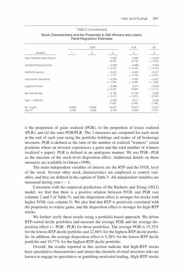
In Table 5, we use the brokerage data to test Barberis and Xiong’s (2012)predictions concerning investors’ propensity to realize gains and the dispositioneffect. We estimate pooled ordinary least squares (OLS) regressions with yearfixed effects, where the dependent variable is one of the following measures:
TABLE 5
Stock Characteristics and the Propensity to Sell Winners and Losers:Panel Regression Estimates
Table 5 reports panel regression (pooled OLS with year fixed effects) estimates, where the dependent variable is 1 ofthe following 3 measures in year t for a given stock: i) proportion of gains realized (PGR) (columns 1–3), ii) proportionof losses realized (PLR) (column 4), and iii) disposition effect (DE) defined as PGR/PLR (column 5). PGR is defined asthe ratio of the number of realized “winners” (stock positions where an investor experiences a gain) and the total numberof winners (realized + paper). PLR is defined in an analogous manner. To ensure that these measures are less noisy,stocks with fewer than 10 trades during a year are excluded. The main independent variables are retail trading proportion(RTP), idiosyncratic volatility (IVOL), and idiosyncratic skewness (ISKEW). RTP is defined as the ratio of the total buy-and sell-initiated small-trades dollar volume and the total market dollar trading volume. The IVOL measure is the varianceof the residual obtained by fitting a 4-factor model (the 3 Fama-French (1993) factors and the momentum factor) to thestock returns time series. ISKEW is defined as the scaled measure of the 3rd moment of the residual obtained by fittinga 2-factor (RMRF and RMRF2) model to the daily returns from the previous 6 months. RMRF is the market return, excessover the risk-free rate. Both measures are estimated for each stock each month using daily returns data. Additionally, thefollowing control variables are employed: i) monthly volume turnover, which is the ratio of the number of shares traded ina month and the number of shares outstanding; ii) firm age, which is the number of years since the stock first appearsin the CRSP database; iii) market beta; iv) firm size; v) book-to-market (BM) ratio; vi) past 12-month stock return; vii) adividend-paying dummy variable, which is set to 1 if the stock pays dividend at least once during the previous 1 year;viii) institutional ownership in the stock; ix) a NASDAQ dummy variable; x) stock price; xi) bid-ask spread; and xii) analystcoverage (ANCOV), which is defined as the number of analysts covering the stock during the past year. All independentvariables are measured during the year t − 1. To ensure that extreme values are not affecting the results, we winsorizeall variables at their 0.5 and 99.5 percentile levels. Both the dependent and the independent variables except the dummyvariables have been standardized (mean is set to 0 and standard deviation is 1) so that the coefficient estimates canbe directly compared within and across specifications. To account for potential serial and cross correlations in errors,we compute firm and year clustered standard errors. The t-statistics, obtained using the corrected standard errors, arereported in parentheses below the estimates. The salient numbers are shown in bold.
PGR PLR DE
Variable 1 2 3 4 5
RTP 0.144 0.042 −0.055 0.060(10.18) (4.34) (−3.12) (4.66)
IVOL 0.224 0.187 −0.052 0.159(15.72) (12.68) (−3.44) (8.35)
ISKEW 0.150 0.130 −0.041 0.087(10.63) (9.51) (−2.51) (9.01)
Monthly Turnover 0.100 0.088 0.049(8.80) (3.98) (3.55)
Firm Age 0.011 0.017 −0.008(2.60) (2.45) (−1.10)
Market Beta 0.027 −0.014 0.019(4.41) (−1.02) (1.65)
log(Firm Size) −0.168 −0.101 −0.140(−6.66) (−5.12) (−4.54)
BM ratio 0.001 −0.020 −0.003(0.062) (−1.32) (−0.46)
(continued on next page)
Han and Kumar 391
TABLE 5 (continued)
Stock Characteristics and the Propensity to Sell Winners and Losers:Panel Regression Estimates
PGR PLR DE
Variable 1 2 3 4 5
Past 12-Month Stock Return 0.035 0.085 −0.042(2.02) (4.78) (−2.50)
Dividend-Paying dummy −0.009 −0.008 −0.004(−0.48) (−0.44) (−0.14)
NASDAQ dummy −0.031 −0.002 −0.011(−1.77) (−0.13) (−0.57)
Institutional Ownership −0.030 −0.007 −0.021(−1.56) (−0.36) (−1.62)
log(Stock Price) −0.094 0.017 −0.029(−3.22) (0.60) (−2.11)
Bid-Ask Spread −0.105 −0.120 0.055(−4.41) (−5.01) (3.35)
log(1 + ANCOV) 0.040 0.011 0.039(1.60) (1.04) (1.66)
No. of obs. 13,856 13,856 13,077 13,077 13,077Adj. R2 0.028 0.059 0.137 0.053 0.071
i) the proportion of gains realized (PGR), ii) the proportion of losses realized(PLR), and iii) the ratio PGR/PLR. The 3 measures are computed for each stockat the end of each year using the portfolio holdings and trades of all brokerageinvestors. PGR is defined as the ratio of the number of realized “winners” (stockpositions where an investor experiences a gain) and the total number of winners(realized + paper). PLR is defined in an analogous manner. We use PGR−PLRas the measure of the stock-level disposition effect. Additional details on thesemeasures are available in Odean (1998).
The main independent variables of interest are the RTP and the IVOL levelof the stock. Several other stock characteristics are employed as control vari-ables, and they are defined in the caption of Table 5. All independent variables aremeasured during year t − 1.
Consistent with the empirical predictions of the Barberis and Xiong (2012)model, we find that there is a positive relation between IVOL and PGR (seecolumns 2 and 3 of Table 5), and the disposition effect is stronger for stocks withhigher IVOL (see column 5). We also find that RTP is positively correlated withthe propensity to realize gains, and the disposition effect is stronger for high-RTPstocks.
We further verify these results using a portfolio-based approach. We defineRTP-sorted decile portfolios and measure the average PGR and the average dis-position effect (= PGR−PLR) for those portfolios. The average PGR is 15.32%for the lowest-RTP decile portfolio and 22.66% for the highest-RTP decile portfo-lio. In addition, the average disposition effect is 5.28% for the lowest-RTP decileportfolio and 10.77% for the highest-RTP decile portfolio.
Overall, the results reported in this section indicate that high-RTP stockshave speculative characteristics and attract the clientele of retail investors who areknown to engage in speculative or gambling-motivated trading. High-RTP stocks

392 Journal of Financial and Quantitative Analysis
are more influenced by the activities of risk-seeking “realization utility” investorsas modeled in Barberis and Xiong (2012).
IV. Speculative Trading and Asset Prices
In this section, we study the asset pricing implications of retail investors’speculative trading activities as captured by the RTP variable. Previous studieshave established both theoretically and empirically that noise trading in gen-eral can have a systematic price impact (e.g., DeLong, Shleifer, Summers, andWaldmann (1990), Kumar and Lee (2006), and Barber et al. (2009)). A key el-ement for noise traders to affect stock prices is limits to arbitrage. As we haveseen, high-RTP stocks tend to have very low market capitalization, low price,high IVOL, low institutional ownership, and low ANCOV. On one hand, wehave shown evidence of speculative, risk-seeking, gambling-motivated trading forhigh-RTP stocks. On the other hand, due to the specific characteristics of high-RTP stocks, they also face high limits to arbitrage such as high transaction costsand high holding costs. These 2 considerations allow the existence of mispricingfor high-RTP stocks.
More specifically, several recent theoretical studies suggest that high-RTPstocks are likely to be overpriced. For example, Scheinkman and Xiong (2003)show that stocks are overpriced when the level of speculative trading is high be-cause of the high resale option value due to large disagreement among investors.Barberis and Huang (2008) show that stocks with high skewness should earn lowaverage returns, because investors with cumulative prospect theory utility over-weight tiny probabilities of large gains. Barberis and Xiong (2012) predict lowaverage return of stocks held and traded primarily by individual investors who areinfluenced by realization utility, such as highly volatile stocks.
Thus, we expect high-RTP stocks to earn low average returns. Furthermore,if the preferences of speculative and realization utility retail investors influencethe negative relation between average stock returns and retail trading, then thisrelation should be stronger (more negative) among stocks with speculative char-acteristics. We test these 2 hypotheses later.
A. RTP and Average Returns: Sorting Results
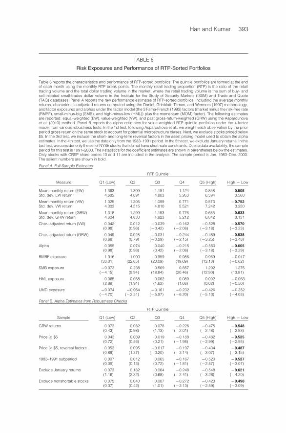
We first examine the relation between the level of retail trading and theaverage stock returns. At the end of each month for the Jan. 1983–Dec. 2000sample period, we form RTP quintile portfolios and compute their equal- andvalue-weighted returns over the next month. The sorting results reported inTable 6 indicate a negative RTP-return relation that is statistically and economi-cally significant.
In particular, the lowest-RTP quintile earns a value-weighted mean monthlyreturn of 1.325%, while the highest-RTP quintile earns a monthly return of only0.573%. The monthly return differential between the 2 extreme value-weightedRTP quintile portfolios (i.e., the RTP premium) is −0.752%, which is economi-cally and statistically significant. The spread between the equal-weighted averagereturns of high- and low-RTP quintiles is −0.505% per month, which is also
Han and Kumar 393
TABLE 6
Risk Exposures and Performance of RTP-Sorted Portfolios
Table 6 reports the characteristics and performance of RTP-sorted portfolios. The quintile portfolios are formed at the endof each month using the monthly RTP break points. The monthly retail trading proportion (RTP) is the ratio of the retailtrading volume and the total dollar trading volume in the market, where the retail trading volume is the sum of buy- andsell-initiated small-trades dollar volume in the Institute for the Study of Security Markets (ISSM) and Trade and Quote(TAQ) databases. Panel A reports the raw performance estimates of RTP-sorted portfolios, including the average monthlyreturns, characteristic-adjusted returns computed using the Daniel, Grinblatt, Titman, and Wermers (1997) methodology,and factor exposures and alphas under the factor model (the 3 Fama-French (1993) factors (market minus the risk-free rate(RMRF), small-minus-big (SMB), and high-minus-low (HML)) plus the momentum (MOM) factor). The following estimatesare reported: equal-weighted (EW), value-weighted (VW), and past gross-return-weighted (GRW) using the Asparouhovaet al. (2010) method. Panel B reports the alpha estimates for value-weighted RTP quintile portfolios under the 4-factormodel from various robustness tests. In the 1st test, following Asparouhova et al., we weight each observation by the priorperiod gross return on the same stock to account for potential microstructure biases. Next, we exclude stocks priced below$5. In the 3rd test, we include the short- and long-term reversal factors in the asset pricing model used to obtain the alphaestimates. In the 4th test, we use the data only from the 1983–1991 period. In the 5th test, we exclude January returns. In thelast test, we consider only the set of NYSE stocks that do not have short-sale constraints. Due to data availability, the sampleperiod for this test is 1991–2000. The t-statistics for the coefficient estimates are shown in parentheses below the estimates.Only stocks with CRSP share codes 10 and 11 are included in the analysis. The sample period is Jan. 1983–Dec. 2000.The salient numbers are shown in bold.
Panel A. Full-Sample Estimates
RTP Quintile
Measure Q1 (Low) Q2 Q3 Q4 Q5 (High) High − Low
Mean monthly return (EW) 1.363 1.309 1.191 1.124 0.858 −0.505Std. dev. EW return 4.682 4.891 4.883 5.263 6.594 3.560
Mean monthly return (VW) 1.325 1.305 1.099 0.771 0.573 −0.752Std. dev. VW return 4.303 4.515 4.810 5.521 7.242 3.350
Mean monthly return (GRW) 1.318 1.299 1.153 0.776 0.685 −0.633Std. dev. GRW return 4.604 4.830 4.823 5.212 6.842 3.131
Char.-adjusted return (VW) 0.042 0.012 −0.039 −0.162 −0.528 −0.570(0.98) (0.96) (−0.42) (−2.06) (−3.18) (−3.23)
Char.-adjusted return (GRW) 0.049 0.028 −0.031 −0.244 −0.489 −0.538(0.68) (0.79) (−0.29) (−2.15) (−3.25) (−3.48)
Alpha 0.055 0.074 0.040 −0.215 −0.550 −0.605(0.98) (0.96) (0.42) (−2.06) (−3.18) (−3.29)
RMRF exposure 1.016 1.000 0.959 0.986 0.969 −0.047(33.01) (22.65) (20.09) (19.69) (13.13) (−0.62)
SMB exposure −0.073 0.238 0.569 0.857 1.202 1.275(−4.15) (9.94) (18.84) (20.46) (12.90) (13.81)
HML exposure 0.065 0.058 0.062 0.089 0.002 −0.063(2.89) (1.91) (1.62) (1.68) (0.02) (−0.50)
UMD exposure −0.074 −0.054 −0.161 −0.232 −0.426 −0.352(−4.70) (−2.51) (−5.97) (−6.20) (−5.13) (−4.03)
Panel B. Alpha Estimates from Robustness Checks
RTP Quintile
Sample Q1 (Low) Q2 Q3 Q4 Q5 (High) High − Low
GRW returns 0.073 0.082 0.078 −0.226 −0.475 −0.548(0.43) (0.98) (1.13) (−2.01) (−2.48) (−2.93)
Price≥ $5 0.043 0.039 0.019 −0.188 −0.482 −0.525(0.72) (0.56) (0.21) (−1.98) (−2.99) (−2.95)
Price≥ $5, reversal factors 0.053 0.095 −0.017 −0.197 −0.434 −0.487(0.89) (1.27) (−0.20) (−2.14) (−3.07) (−3.15)
1983–1991 subperiod 0.007 0.012 0.065 −0.167 −0.520 −0.527(0.09) (0.13) (0.72) (−1.81) (−2.87) (−3.07)
Exclude January returns 0.073 0.182 0.064 −0.248 −0.548 −0.621(1.16) (2.32) (0.68) (−2.41) (−3.26) (−4.20)
Exclude nonshortable stocks 0.075 0.040 0.087 −0.272 −0.423 −0.498(0.37) (0.42) (1.01) (−2.13) (−2.89) (−3.09)
394 Journal of Financial and Quantitative Analysis
significant. The characteristic-adjusted performance estimates and the 4-factor(Fama-French (1993) 3 factors plus a momentum factor) alpha estimates portraya very similar picture. The annualized characteristic- and risk-adjusted RTP pre-mium estimates are both about −7%. All these results remain about the samewhen we follow the Asparouhova et al. (2010) method to account for potentialmicrostructure noise by using gross returns from the previous period to weightthe observations.
Panel B of Table 6 indicates that the negative RTP-average return relationis robust. For example, when we exclude stocks with a price below $5 to ensurethat microstructure effects (e.g., large bid-ask spreads) are not driving our results,the top RTP quintile still underperforms the low-RTP quintile on average by astatistically significant 0.525% per month. The negative RTP premium remainssignificant even when we add the short- and long-term reversal factors in the assetpricing model used to obtain the risk-adjusted performance estimates.
It is useful to note a robust pattern in Table 6. The characteristics- or risk-adjusted mean returns of high-RTP portfolios are negative and statistically signifi-cant, while those of the low-RTP portfolios are positive but insignificant. Thus, thenegative RTP premium is exclusively due to the underperformance of high-RTPstocks and not due to the overperformance of low-RTP stocks. High-RTP stocks,that is, those whose trading is dominated by retail investors, tend to be over-priced. This fits well with the high contemporaneous return of the high-RTPstocks (see Table 1). It is consistent with the pricing impact of noise traders forhigh-RTP stocks, because these stocks not only are dominated by retail investors;they also face high limits to arbitrage such as short-sale constraints.
However, our results cannot be completely explained by short-sale constraints.When we consider only the set of NYSE stocks that do not have short-sale con-straints, we still find that the top RTP quintile has a significant negative alphaof −0.423% per month (last row of Panel B in Table 6). This is consistent withthe implications of equilibrium models such as Barberis and Huang (2008) andBarberis and Xiong (2012) that do not require short-sale constraints. The−0.423%alpha of high-RTP stocks without short-sale constraints is less negative than the−0.55% alpha for the high-RTP stocks in the full sample. This supports the ideathat short-sale constraints exacerbate the pricing impact of speculative trading.
Figure 2 plots the raw monthly return difference between the high(top-quintile) RTP and low (bottom-quintile) RTP portfolios and the 12-monthmoving average of the monthly return differentials. The high-RTP stocks under-perform low-RTP stocks consistently, as the return differential is negative for mostof the months during our sample period. While the return differential between thehigh-RTP and low-RTP stocks becomes larger in magnitude during the NASDAQbubble period, our results are not driven by this period. The RTP-sorting resultsreported in Panel B of Table 6 also show that our results are similar when weuse the data only from the 1st half of the sample period (1983–1991) or when weexclude January returns. Thus, the profits of RTP-based trading strategies are notlimited to a few specific time periods.
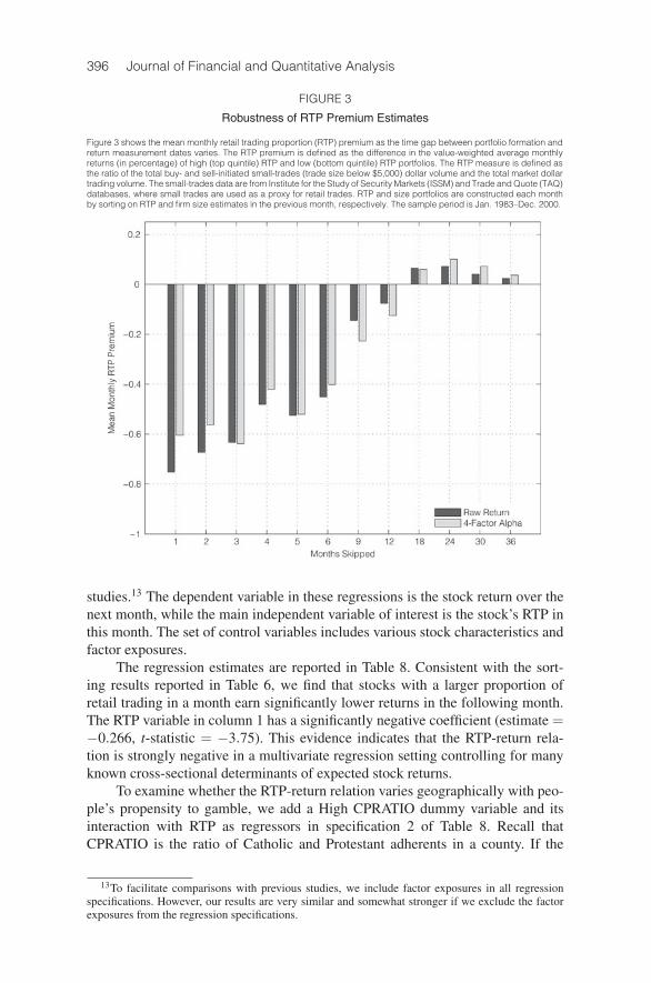
Figure 3 illustrates how the return differences between the high-RTP stocksand low-RTP stocks vary with the time gap between portfolio formation andreturn measurement dates. We find that the return difference (i.e., RTP premium)

Han and Kumar 395
FIGURE 2
RTP Premium Time Series
Figure 2 shows the monthly retail trading proportion (RTP) premium, defined as the difference in the value-weighted averagemonthly returns (in percentage) of high (top quintile) RTP and low (bottom quintile) RTP portfolios. Both the raw and the12-month backward moving average time series are plotted. The RTP measure is defined as the ratio of the total buy- andsell-initiated small-trades (trade size below $5,000) dollar volume and the total market dollar trading volume. The small-trades data are from Institute for the Study of Security Markets (ISSM) and Trade and Quote (TAQ) databases, where smalltrades are used as a proxy for retail trades. RTP portfolios are constructed each month by sorting on RTP estimates inthe previous month. In any given month, stocks priced below $5 are excluded from the sample. The sample period isJan. 1983–Dec. 2000.
becomes smaller as the time gap widens. The RTP premium is significant whenthe gap between the 2 dates is up to 6 months. It is only weakly significant whenwe skip about 9 months. The RTP premium estimates eventually lose significanceand even switch signs when we skip more than 12 months.
The evidence in Table 7 shows that the RTP premium is larger in magnitudeamong smaller stocks. Panel A presents the raw returns, while Panel B reportsthe 4-factor alpha estimates for the value-weighted portfolios.12 For the top 2NYSE firm size quintiles, the average monthly RTP premium is statistically weakor insignificant. This evidence adds support to the view that the RTP premiumreflects the pricing impact of speculative retail trading, since the concentration ofspeculative retail trading is higher among smaller stocks.
B. Fama-MacBeth Regression Estimates
We characterize the influence of retail trading on stock returns more ac-curately by estimating a series of monthly Fama-MacBeth (1973) regressions,where the regression specification is motivated by AHXZ (2009) and other related
12The results are qualitatively very similar when we consider equal-weighted or gross-return-weighted portfolios.
396 Journal of Financial and Quantitative Analysis
FIGURE 3
Robustness of RTP Premium Estimates
Figure 3 shows the mean monthly retail trading proportion (RTP) premium as the time gap between portfolio formation andreturn measurement dates varies. The RTP premium is defined as the difference in the value-weighted average monthlyreturns (in percentage) of high (top quintile) RTP and low (bottom quintile) RTP portfolios. The RTP measure is defined asthe ratio of the total buy- and sell-initiated small-trades (trade size below $5,000) dollar volume and the total market dollartrading volume. The small-trades data are from Institute for the Study of Security Markets (ISSM) and Trade and Quote (TAQ)databases, where small trades are used as a proxy for retail trades. RTP and size portfolios are constructed each monthby sorting on RTP and firm size estimates in the previous month, respectively. The sample period is Jan. 1983–Dec. 2000.
studies.13 The dependent variable in these regressions is the stock return over thenext month, while the main independent variable of interest is the stock’s RTP inthis month. The set of control variables includes various stock characteristics andfactor exposures.
The regression estimates are reported in Table 8. Consistent with the sort-ing results reported in Table 6, we find that stocks with a larger proportion ofretail trading in a month earn significantly lower returns in the following month.The RTP variable in column 1 has a significantly negative coefficient (estimate =−0.266, t-statistic = −3.75). This evidence indicates that the RTP-return rela-tion is strongly negative in a multivariate regression setting controlling for manyknown cross-sectional determinants of expected stock returns.
To examine whether the RTP-return relation varies geographically with peo-ple’s propensity to gamble, we add a High CPRATIO dummy variable and itsinteraction with RTP as regressors in specification 2 of Table 8. Recall thatCPRATIO is the ratio of Catholic and Protestant adherents in a county. If the
13To facilitate comparisons with previous studies, we include factor exposures in all regressionspecifications. However, our results are very similar and somewhat stronger if we exclude the factorexposures from the regression specifications.

Han and Kumar 397
TABLE 7
Performance of RTP and Firm Size Double-Sorted Portfolios
Table 7 reports the mean monthly performance of firm size and retail trading proportion (RTP) sorted portfolios. At the endof each month, we first sort firms based on NYSE size quintiles and then sort firms within each of the NYSE size quintilesinto 5 RTP quintiles. RTP and size portfolios are constructed each month by sorting on RTP and firm size estimates in theprevious month, respectively. The monthly RTP is the ratio of the retail trading volume and the total dollar trading volumein the market, where the retail trading volume is the sum of buy- and sell-initiated small-trades dollar volume in the Institutefor the Study of Security Markets (ISSM) and Trade and Quote (TAQ) databases. Firm size is defined as the product ofnumber of shares outstanding and end-of-month stock price. Panel A reports the raw performance estimates and Panel Breports the 4-factor model alpha estimates for those value-weighted portfolios. The t-statistics for the coefficient estimatesare shown in parentheses below the estimates. Only stocks with CRSP share codes 10 and 11 are included in the analysis.The sample period is Jan. 1983–Dec. 2000. The salient numbers are shown in bold.
RTP Quintile
NYSE Size Quintile All Q1 (Low) Q2 Q3 Q4 Q5 (High) High − Low
Panel A. Mean Monthly Returns
All 1.325 1.305 1.099 0.771 0.573 −0.752(−3.88)
Q1 (low) 1.051 1.273 1.259 1.024 0.669 0.221 −1.052(−4.01)
Q2 1.182 1.281 1.334 1.042 0.732 0.310 −0.971(−3.77)
Q3 1.234 1.312 1.242 1.106 0.805 0.679 −0.633(−2.82)
Q4 1.317 1.345 1.132 1.122 1.025 0.990 −0.355(−2.12)
Q5 (high) 1.384 1.413 1.387 1.375 1.269 1.283 −0.130(−1.08)
Panel B. 4-Factor Alpha Estimates
All 0.055 0.074 0.040 −0.215 −0.550 −0.605(0.98) (0.96) (0.42) (−2.06) (−3.18) (−3.29)
Q1 (low) −0.122 −0.050 −0.074 −0.104 −0.506 −0.922 −0.972(−1.26) (−0.69) (−0.98) (−0.77) (−3.15) (−4.01) (−3.62)
Q2 −0.032 0.025 0.044 −0.094 −0.450 −0.729 −0.754(−0.53) (0.53) (1.26) (−1.01) (−2.58) (−3.02) (−2.72)
Q3 0.019 0.026 0.024 −0.076 −0.304 −0.415 −0.441(0.53) (0.26) (0.28) (−1.05) (−1.88) (−2.19) (−2.57)
Q4 0.007 0.049 0.040 −0.084 −0.109 −0.171 −0.220(0.09) (1.42) (0.68) (−1.04) (−1.62) (−1.85) (−1.74)
Q5 (high) 0.086 0.107 0.099 0.097 0.023 0.024 −0.083(2.84) (2.69) (1.65) (1.47) (0.54) (0.40) (−0.81)
negative RTP-return relation is driven by speculative retail trading, then it shouldbe even more negative when a firm is headquartered in (and hence many of itsinvestors come from) a county where gambling activities are more acceptable.In other words, we expect the interaction term to have a negative coefficient es-timate if the local gambling environment as captured by CPRATIO influencesthe RTP-return relation. The estimates reported in column 2 confirm that theRTP × High CPRATIO coefficient is significantly negative (estimate = −0.071,t-statistic = −2.41). This evidence indicates that the magnitude of the negativeRTP premium is higher for firms that are located in high-CPRATIO regions, againsupporting our view that the negative RTP premium reflects the pricing impact ofspeculative retail trading.
In specifications 3 and 4 of Table 8, we add 4 control variables to accountfor other potential determinants of average returns: the past 1-month return toaccount for short-term reversal, the level of institutional ownership, retail BSI

398 Journal of Financial and Quantitative Analysis
TABLE 8
Retail Trading and Average Returns:Fama-MacBeth Cross-Sectional Regression Estimates
Table 8 reports the estimates from monthly Fama-MacBeth (1973) cross-sectional regressions, where the monthly stockreturn is the dependent variable. The dependent variable is the raw monthly return in columns 1–3. In column 4, followingAsparouhova et al. (2010), we use the past gross-return-weighted monthly return as the dependent variable. The mainindependent variable is a measure of retail trading (RTP) at the end of the previous month. The monthly RTP is the ratioof the retail trading volume and the total dollar trading volume, where the retail trading volume is the sum of buy- andsell-initiated small-trades dollar volume in the Institute for the Study of Security Markets (ISSM) and Trade and Quote (TAQ)databases. Other independent variables are the 3 factor exposures (market, small-minus-big (SMB), and high-minus-low(HML) betas), and various firm characteristics (firm size, book-to-market (BM) ratio, past 6-month return, and stock price).The factor exposures are measured “contemporaneously,” firm size and 6-month returns are measured in the previousmonth, and the BM measure is from 6 months ago. In some specifications, we also consider the past 1-month stock return,the level of institutional ownership (IO), retail buy-sell imbalance (BSI), and the illiquidity measure of Amihud (2002), definedas the absolute daily returns per unit of trading volume. All regression specifications use the time period for which the retailtrading data are available (1983–2000). The sample period is Jan. 1983–Dec. 2000 in all columns. We follow the Pontiff(1996) methodology to correct the Fama-MacBeth standard errors for potential serial correlation. The t-statistics for thecoefficient estimates are shown in parentheses below the estimates. To ensure that extreme values are not affecting theresults, we winsorize all variables at their 0.5 and 99.5 percentile levels. All independent variables are standardized suchthat each variable has a mean of 0 and a standard deviation of 1. Only stocks with CRSP share codes 10 and 11 areincluded in the analysis. The salient numbers are shown in bold.
Dependent variable is the return of stock i in month t.
Variable 1 2 3 4
log(RTP) −0.266 −0.295 −0.388 −0.326(−3.75) (−3.54) (−4.77) (−3.59)
log(RTP)× High CPRATIO −0.066 −0.082 −0.079(−2.07) (−3.23) (−3.11)
High CPRATIO −0.024 0.011 −0.008(−1.26) (−1.45) (−0.32)
Market Beta 0.970 0.972 0.910 0.994(4.84) (4.88) (3.95) (5.03)
SMB Beta 0.085 0.086 0.097 0.066(0.67) (0.68) (1.47) (0.81)
HML Beta −0.410 −0.408 −0.403 −0.336(−2.74) (−2.89) (−2.06) (−2.55)
log(Firm Size) −0.367 −0.371 −0.306 −0.367(−3.14) (−3.15) (−3.17) (−3.26)
BM 0.247 0.250 0.325 0.232(3.49) (3.57) (4.05) (3.49)
Past 6-Month Return 0.011 0.012 0.311 0.231(0.52) (0.81) (3.65) (2.87)
log(Stock Price) −0.145 −0.143 −0.150 −0.367(−2.20) (−2.25) (−2.67) (−3.26)
Past 1-Month Return −0.506(−5.70)
BSI 0.388 0.329(5.24) (3.43)
IO −0.018 −0.006(−0.74) (−0.25)
Amihud Illiquidity −0.003 −0.032(−0.14) (−0.56)
Intercept 1.405 1.404 1.412 1.156(3.29) (3.03) (3.07) (3.73)
Avg. no. of stocks 4,593 4,593 4,593 4,584Avg. adj. R2 0.048 0.050 0.059 0.041
(Barber et al. (2009)), and the Amihud (2002) illiquidity measure. We includethe retail BSI measure in the specification to examine whether our RTP measurereflects the findings of Kaniel et al. (2008) and Barber et al. (2009), who showthat stocks heavily bought by individuals 1 week reliably outperform the market
Han and Kumar 399
the following week.14 The institutional ownership variable accounts for the possi-bility that RTP simply reflects the effects of institutional ownership. Specifically,RTP may negatively forecast future returns of stocks because institutions are moreinformed and better at identifying stocks that would perform well in the future.Therefore, stocks with low institutional ownership (which would have high RTP)would have lower average future returns.
In the extended regression specification reported in column 3 of Table 8, wefind that the past 1-month stock return has a strongly negative coefficient estimate,which is consistent with the evidence in Huang, Liu, Ghee, and Zhang (2010).Furthermore, consistent with the evidence in Barber et al. (2009), we find thatBSI has a significantly positive coefficient estimate. In contrast, the institutionalownership and illiquidity variables have insignificant coefficient estimates.
More importantly, we find that both RTP and RTP × High CPRATIO coef-ficient estimates remain significantly negative in the presence of these additionalcontrol variables. Those estimates also maintain their significance when we runa weighted least squares regression (see column 4 of Table 8). In this specifica-tion, we follow Asparouhova et al. (2010) and define weights based on the grossstock return in the previous month. Overall, the results from our extended speci-fications indicate that RTP does not merely reflect the short-term return reversaleffect (e.g., Jegadeesh (1990), Lehmann (1990)) or the known effects of retailtrading imbalance, institutional ownership, and liquidity on stock returns.
C. Negative RTP Premium among Speculative Stocks
In Table 9, we test our 2nd hypothesis that the RTP-return relation is strongeramong stocks with speculative characteristics. To do so, we include the interactionof RTP with 2 speculative stock characteristics, namely, IVOL and LOTT in theregressions. The interaction terms would have significantly negative coefficientestimates if the RTP-return relation gets amplified for the subset of speculativestocks.
The regression estimates reported in Table 9 confirm that there is a negativepremium associated with both the IVOL and the LOTT variables. Both the IVOLand the LOTT coefficient estimates are significantly negative, where the IVOLcoefficient estimate is consistent with the evidence in AHXZ (2009). More im-portantly, we find that high-RTP stocks underperform by a larger amount if theyhave higher volatility or have stronger lottery features. Both the High RTP×HighIVOL and High RTP × High LOTT coefficient estimates are significantly nega-tive. For example, in column 3, the coefficient for the High RTP dummy variableindicates that stocks ranked in the top 1/3 by RTP is associated with a −0.308%reduction in the mean monthly stock return. This effect is amplified for stockswith high IVOL. The coefficient estimate of the interaction term indicates that theaverage monthly return on the high-IVOL stocks on average underperforms by
14BSI is related to our RTP measure, but there are significant differences. A stock can have a lowlevel of retail trading, but the retail trades could be mostly on the same side, which implies a large(either positive or negative) BSI. There can also be a high level of retail trading in a stock but low BSI.We find that the average cross-sectional correlation between RTP and BSI is only 0.091.
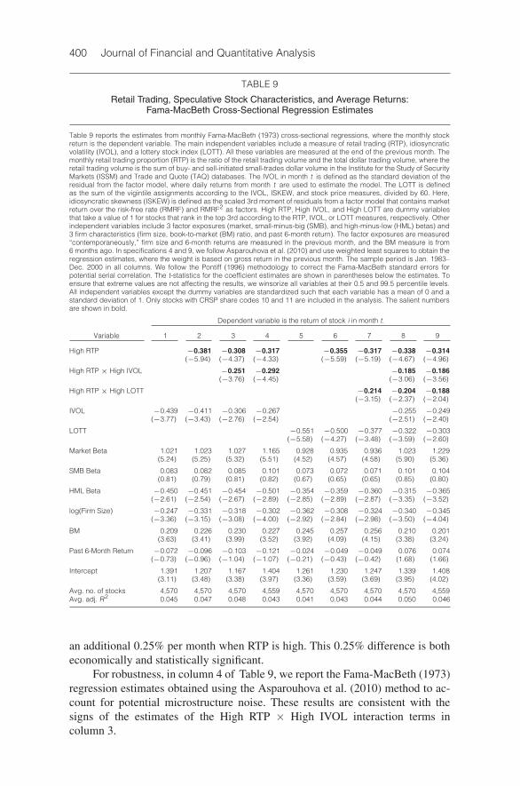
400 Journal of Financial and Quantitative Analysis
TABLE 9
Retail Trading, Speculative Stock Characteristics, and Average Returns:Fama-MacBeth Cross-Sectional Regression Estimates
Table 9 reports the estimates from monthly Fama-MacBeth (1973) cross-sectional regressions, where the monthly stockreturn is the dependent variable. The main independent variables include a measure of retail trading (RTP), idiosyncraticvolatility (IVOL), and a lottery stock index (LOTT). All these variables are measured at the end of the previous month. Themonthly retail trading proportion (RTP) is the ratio of the retail trading volume and the total dollar trading volume, where theretail trading volume is the sum of buy- and sell-initiated small-trades dollar volume in the Institute for the Study of SecurityMarkets (ISSM) and Trade and Quote (TAQ) databases. The IVOL in month t is defined as the standard deviation of theresidual from the factor model, where daily returns from month t are used to estimate the model. The LOTT is definedas the sum of the vigintile assignments according to the IVOL, ISKEW, and stock price measures, divided by 60. Here,idiosyncratic skewness (ISKEW) is defined as the scaled 3rd moment of residuals from a factor model that contains marketreturn over the risk-free rate (RMRF) and RMRF2 as factors. High RTP, High IVOL, and High LOTT are dummy variablesthat take a value of 1 for stocks that rank in the top 3rd according to the RTP, IVOL, or LOTT measures, respectively. Otherindependent variables include 3 factor exposures (market, small-minus-big (SMB), and high-minus-low (HML) betas) and3 firm characteristics (firm size, book-to-market (BM) ratio, and past 6-month return). The factor exposures are measured“contemporaneously,” firm size and 6-month returns are measured in the previous month, and the BM measure is from6 months ago. In specifications 4 and 9, we follow Asparouhova et al. (2010) and use weighted least squares to obtain theregression estimates, where the weight is based on gross return in the previous month. The sample period is Jan. 1983–Dec. 2000 in all columns. We follow the Pontiff (1996) methodology to correct the Fama-MacBeth standard errors forpotential serial correlation. The t-statistics for the coefficient estimates are shown in parentheses below the estimates. Toensure that extreme values are not affecting the results, we winsorize all variables at their 0.5 and 99.5 percentile levels.All independent variables except the dummy variables are standardized such that each variable has a mean of 0 and astandard deviation of 1. Only stocks with CRSP share codes 10 and 11 are included in the analysis. The salient numbersare shown in bold.
Dependent variable is the return of stock i in month t.
Variable 1 2 3 4 5 6 7 8 9
High RTP −0.381 −0.308 −0.317 −0.355 −0.317 −0.338 −0.314(−5.94) (−4.37) (−4.33) (−5.59) (−5.19) (−4.67) (−4.96)
High RTP× High IVOL −0.251 −0.292 −0.185 −0.186(−3.76) (−4.45) (−3.06) (−3.56)
High RTP× High LOTT −0.214 −0.204 −0.188(−3.15) (−2.37) (−2.04)
IVOL −0.439 −0.411 −0.306 −0.267 −0.255 −0.249(−3.77) (−3.43) (−2.76) (−2.54) (−2.51) (−2.40)
LOTT −0.551 −0.500 −0.377 −0.322 −0.303(−5.58) (−4.27) (−3.48) (−3.59) (−2.60)
Market Beta 1.021 1.023 1.027 1.165 0.928 0.935 0.936 1.023 1.229(5.24) (5.25) (5.32) (5.51) (4.52) (4.57) (4.58) (5.90) (5.36)
SMB Beta 0.083 0.082 0.085 0.101 0.073 0.072 0.071 0.101 0.104(0.81) (0.79) (0.81) (0.82) (0.67) (0.65) (0.65) (0.85) (0.80)
HML Beta −0.450 −0.451 −0.454 −0.501 −0.354 −0.359 −0.360 −0.315 −0.365(−2.61) (−2.54) (−2.67) (−2.89) (−2.85) (−2.89) (−2.87) (−3.35) (−3.52)
log(Firm Size) −0.247 −0.331 −0.318 −0.302 −0.362 −0.308 −0.324 −0.340 −0.345(−3.36) (−3.15) (−3.08) (−4.00) (−2.92) (−2.84) (−2.98) (−3.50) (−4.04)
BM 0.209 0.226 0.230 0.227 0.245 0.257 0.256 0.210 0.201(3.63) (3.41) (3.99) (3.52) (3.92) (4.09) (4.15) (3.38) (3.24)
Past 6-Month Return −0.072 −0.096 −0.103 −0.121 −0.024 −0.049 −0.049 0.076 0.074(−0.73) (−0.96) (−1.04) (−1.07) (−0.21) (−0.43) (−0.42) (1.68) (1.66)
Intercept 1.391 1.207 1.167 1.404 1.261 1.230 1.247 1.339 1.408(3.11) (3.48) (3.38) (3.97) (3.36) (3.59) (3.69) (3.95) (4.02)
Avg. no. of stocks 4,570 4,570 4,570 4,559 4,570 4,570 4,570 4,570 4,559Avg. adj. R2 0.045 0.047 0.048 0.043 0.041 0.043 0.044 0.050 0.046
an additional 0.25% per month when RTP is high. This 0.25% difference is botheconomically and statistically significant.
For robustness, in column 4 of Table 9, we report the Fama-MacBeth (1973)regression estimates obtained using the Asparouhova et al. (2010) method to ac-count for potential microstructure noise. These results are consistent with thesigns of the estimates of the High RTP × High IVOL interaction terms incolumn 3.
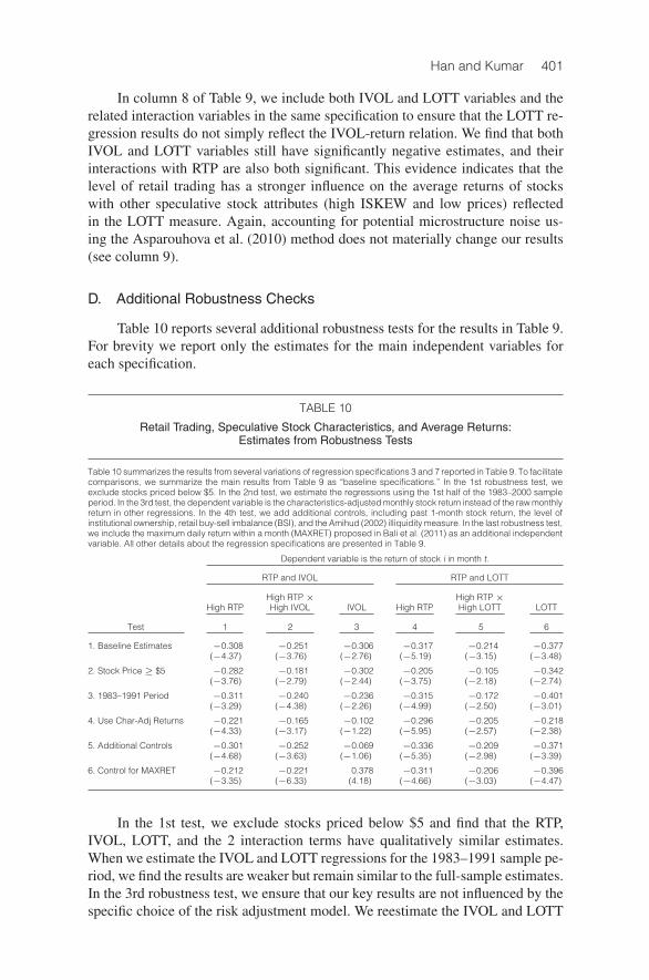
Han and Kumar 401
In column 8 of Table 9, we include both IVOL and LOTT variables and therelated interaction variables in the same specification to ensure that the LOTT re-gression results do not simply reflect the IVOL-return relation. We find that bothIVOL and LOTT variables still have significantly negative estimates, and theirinteractions with RTP are also both significant. This evidence indicates that thelevel of retail trading has a stronger influence on the average returns of stockswith other speculative stock attributes (high ISKEW and low prices) reflectedin the LOTT measure. Again, accounting for potential microstructure noise us-ing the Asparouhova et al. (2010) method does not materially change our results(see column 9).
D. Additional Robustness Checks
Table 10 reports several additional robustness tests for the results in Table 9.For brevity we report only the estimates for the main independent variables foreach specification.
TABLE 10
Retail Trading, Speculative Stock Characteristics, and Average Returns:Estimates from Robustness Tests
Table 10 summarizes the results from several variations of regression specifications 3 and 7 reported in Table 9. To facilitatecomparisons, we summarize the main results from Table 9 as “baseline specifications.” In the 1st robustness test, weexclude stocks priced below $5. In the 2nd test, we estimate the regressions using the 1st half of the 1983–2000 sampleperiod. In the 3rd test, the dependent variable is the characteristics-adjusted monthly stock return instead of the raw monthlyreturn in other regressions. In the 4th test, we add additional controls, including past 1-month stock return, the level ofinstitutional ownership, retail buy-sell imbalance (BSI), and the Amihud (2002) illiquidity measure. In the last robustness test,we include the maximum daily return within a month (MAXRET) proposed in Bali et al. (2011) as an additional independentvariable. All other details about the regression specifications are presented in Table 9.
Dependent variable is the return of stock i in month t.
RTP and IVOL RTP and LOTT
High RTP× High RTP×High RTP High IVOL IVOL High RTP High LOTT LOTT
Test 1 2 3 4 5 6
1. Baseline Estimates −0.308 −0.251 −0.306 −0.317 −0.214 −0.377(−4.37) (−3.76) (−2.76) (−5.19) (−3.15) (−3.48)
2. Stock Price≥ $5 −0.282 −0.181 −0.302 −0.205 −0.105 −0.342(−3.76) (−2.79) (−2.44) (−3.75) (−2.18) (−2.74)
3. 1983–1991 Period −0.311 −0.240 −0.236 −0.315 −0.172 −0.401(−3.29) (−4.38) (−2.26) (−4.99) (−2.50) (−3.01)
4. Use Char-Adj Returns −0.221 −0.165 −0.102 −0.296 −0.205 −0.218(−4.33) (−3.17) (−1.22) (−5.95) (−2.57) (−2.38)
5. Additional Controls −0.301 −0.252 −0.069 −0.336 −0.209 −0.371(−4.68) (−3.63) (−1.06) (−5.35) (−2.98) (−3.39)
6. Control for MAXRET −0.212 −0.221 0.378 −0.311 −0.206 −0.396(−3.35) (−6.33) (4.18) (−4.66) (−3.03) (−4.47)
In the 1st test, we exclude stocks priced below $5 and find that the RTP,IVOL, LOTT, and the 2 interaction terms have qualitatively similar estimates.When we estimate the IVOL and LOTT regressions for the 1983–1991 sample pe-riod, we find the results are weaker but remain similar to the full-sample estimates.In the 3rd robustness test, we ensure that our key results are not influenced by thespecific choice of the risk adjustment model. We reestimate the IVOL and LOTT
402 Journal of Financial and Quantitative Analysis
regressions using characteristic-adjusted returns, where we also control for riskby including the factor exposures in the regression specification. Again, we findthat all key independent variables maintain their statistical significance levels andtheir signs.
In the last 2 robustness tests, we include additional control variables in the re-gression specifications. When we include past 1-month stock return, institutionalownership, retail BSI, and Amihud (2002) illiquidity measure in the specifica-tion, the High RTP and High RTP × High IVOL remain significantly negative inboth IVOL and LOTT regression specifications. However, consistent with the evi-dence in Huang et al. (2010), we find that IVOL loses its statistical significance.15
In contrast, the LOTT variables remain significantly negative even in the presenceof a control for the short-term reversal effect.
When we include the maximum daily return within a month (MAXRET)measure proposed in Bali, Cakici, and Whitelaw (2011) as an additional indepen-dent variable, consistent with their evidence, the IVOL coefficient estimate be-comes positive. However, again, the LOTT variable remains significantly negativeeven in the presence of MAXRET. Furthermore, the High RTP× High IVOL andHigh RTP× High LOTT interaction terms continue to have significantly negativecoefficient estimates. This evidence indicates that although the volatility-returnrelation switches sign in the presence of MAXRET, stocks with high IVOL con-tinue to earn lower incremental returns when the level of retail trading is high.Furthermore, this evidence indicates that the MAXRET measure does not alterthe negative relation between the LOTT and stock returns.
V. Summary and Conclusion
In this paper, we introduce the retail trading proportion (RTP) variable forindividual stocks constructed from their trading records and show that it effec-tively captures the speculative trading activities of retail investors. Stocks withlottery features (high volatility, high skewness, and low prices) are heavily tradedby retail investors and, thus, have high RTP, while institutions underweight thosestocks. Furthermore, the characteristics of the retail clienteles of high-RTP stocksare remarkably similar to the characteristics of investors who are attracted tolottery-type stocks (Kumar (2009)). RTP is also high for firms that are head-quartered in regions where people exhibit a greater propensity to gamble. Andconsistent with the realization utility model of Barberis and Xiong (2012), weshow that investors’ propensity to realize gains is stronger among high-volatilitystocks and stocks with high levels of retail trading.
Examining the asset pricing implications of speculative retail trading, we findthat high-RTP stocks tend to be overpriced. We show that stocks with high levelsof retail trading significantly underperform low-retail-trading stocks, where thehigh-low RTP return differential (i.e., the RTP premium) is about −7% annually.The negative RTP premium is stronger among stocks that have lottery features orare located in regions in which people exhibit a stronger propensity to gamble.
15Huang et al. (2010) show that the volatility-return relation is insignificant when past 1-monthreturn is used as a control variable.

Han and Kumar 403
Our results are consistent with noise trader models in general, and in particular,several recent behavioral models that show that investors’ willingness to pay apremium for stocks with lottery features and high realization utility potential cancause mispricing for these stocks (e.g., Barberis and Huang (2008), Barberis andXiong (2012)).
Taken together, our empirical findings contribute to the recent retail investorliterature, which documents that retail trading can affect stock prices and forecastfuture stock returns (e.g., Kumar and Lee (2006), Barber et al. (2009), Dorn et al.(2008), Hvidkjaer (2008), and Kaniel et al. (2008)). The evidence also highlightsthe usefulness of a habitat-based approach for studying asset prices. Future re-search may find it fruitful to examine whether our retail clientele proxy can helpexplain other related asset pricing anomalies such as the negative relation betweendistress risk and stock returns.
ReferencesAmihud, Y. “Illiquidity and Stock Returns: Cross-Section and Time-Series Effects.” Journal of Fi-
nancial Markets, 5 (2002), 31–56.Ang, A.; R. J. Hodrick; Y. Xing; and X. Zhang. “The Cross-Section of Volatility and Expected Re-
turns.” Journal of Finance, 61 (2006), 259–299.Ang, A.; R. J. Hodrick; Y. Xing; and X. Zhang. “High Idiosyncratic Volatility and Low Returns:
International and Further U.S. Evidence.” Journal of Financial Economics, 91 (2009), 1–23.Asparouhova, E.; H. Bessembinder; and I. Kalcheva. “Liquidity Biases in Asset Pricing Tests.” Jour-
nal of Financial Economics, 96 (2010), 215–237.Badrinath, S. G.; G. D. Gay; and J. R. Kale. “Patterns of Institutional Investment, Prudence, and the
Managerial ‘Safety-Net’ Hypothesis.” Journal of Risk and Insurance, 56 (1989), 605–629.Bali, T. G.; N. Cakici; and R. Whitelaw. “Maxing Out: Stocks as Lotteries and the Cross-Section of
Expected Returns.” Journal of Financial Economics, 99 (2011), 427–446.Barber, B. M., and T. Odean. “Trading Is Hazardous to Your Wealth: The Common Stock Investment
Performance of Individual Investors.” Journal of Finance, 55 (2000), 773–806.Barber, B. M.; T. Odean; and N. Zhu. “Do Retail Trades Move Markets?” Review of Financial Studies,
22 (2009), 151–186.Barberis, N., and M. Huang. “Stocks as Lotteries: The Implications of Probability Weighting for
Security Prices.” American Economic Review, 98 (2008), 2066–2100.Barberis, N., and W. Xiong. “Realization Utility.” Journal of Financial Economics, 104 (2012), 251–
271.Battalio, R. H., and R. R. Mendenhall. “Earnings Expectations, Investor Trade Size, and Anomalous
Returns Around Earnings Announcements.” Journal of Financial Economics, 77 (2005), 289–319.Daniel, K. D.; M. Grinblatt; S. Titman; and R. Wermers. “Measuring Mutual Fund Performance with
Characteristic-Based Benchmarks.” Journal of Finance, 52 (1997), 1035–1058.Del Guercio, D. “The Distorting Effect of the Prudent Man Law on Institutional Equity Investments.”
Journal of Financial Economics, 40 (1996), 31–62.DeLong, J. B.; A. Shleifer; L. H. Summers; and R. J. Waldmann. “Noise Trader Risk in Financial
Markets.” Journal of Political Economy, 98 (1990), 703–738.Dorn, D., and G. Huberman. “Preferred Risk Habitat of Individual Investors.” Journal of Financial
Economics, 97 (2010), 155–173.Dorn, D.; G. Huberman; and P. Sengmueller. “Correlated Trading and Returns.” Journal of Finance,
63 (2008), 885–920.Dorn, D., and P. Sengmueller. “Trading as Entertainment.” Management Science, 55 (2009), 591–603.Fama, E. F., and K. R. French. “Common Risk Factors in the Returns on Stocks and Bonds.” Journal
of Financial Economics, 33 (1993), 3–56.Fama, E. F., and J. D. MacBeth. “Risk, Return, and Equilibrium: Empirical Tests.” Journal of Political
Economy, 81 (1973), 607–636.Grinblatt, M., and M. Keloharju. “Sensation Seeking, Overconfidence, and Trading Activity.” Journal
of Finance, 64 (2009), 549–578.Harvey, C. R., and A. Siddique. “Conditional Skewness in Asset Pricing Tests.” Journal of Finance,
55 (2000), 1263–1295.

404 Journal of Financial and Quantitative Analysis
Huang, W.; Q. Liu; S. R. Ghee; and L. Zhang. “Return Reversals, Idiosyncratic Risk and ExpectedReturns.” Review of Financial Studies, 24 (2010), 147–168.
Hvidkjaer, S. “Small Trades and the Cross-Section of Stock Returns.” Review of Financial Studies, 21(2008), 1123–1151.
Jegadeesh, N. “Evidence of Predictable Behavior of Security Returns.” Journal of Finance, 45 (1990),881–898.
Kaniel, R.; G. Saar; and S. Titman. “Individual Investor Trading and Stock Returns.” Journal ofFinance, 63 (2008), 273–310.
Kumar, A. “Who Gambles in the Stock Market?” Journal of Finance, 64 (2009), 1889–1933.Kumar, A., and C. M. C. Lee. “Retail Investor Sentiment and Return Comovements.” Journal of Fi-
nance, 61 (2006), 2451–2486.Kumar, A.; J. Page; and O. Spalt. “Religious Beliefs, Gambling Attitudes, and Financial Market
Outcomes.” Journal of Financial Economics, 102 (2011), 671–708.Lee, C. M. C., and B. Radhakrishna. “Inferring Investor Behavior: Evidence from TORQ Data.” Jour-
nal of Financial Markets, 3 (2000), 83–111.Lehmann, B. N. “Fads, Martingales, and Market Efficiency.” Quarterly Journal of Economics, 105
(1990), 1–28.Malmendier, U., and D. M. Shanthikumar. “Are Small Investors Naive About Incentives?” Journal of
Financial Economics, 85 (2007), 457–489.Odean, T. “Are Investors Reluctant to Realize Their Losses?” Journal of Finance, 53 (1998), 1775–
1798.Pontiff, J. “Costly Arbitrage: Evidence from Closed-End Funds.” Quarterly Journal of Economics,
111 (1996), 1135–1151.Scheinkman, J. A., and W. Xiong. “Overconfidence and Speculative Bubbles.” Journal of Political
Economy, 111 (2003), 1183–1219.Shefrin, H. M., and M. Statman. “Behavioral Portfolio Theory.” Journal of Financial and Quantitative
Analysis, 35 (2000), 127–151.