“Speculative Influence Network” during financialbubbles: application to Chinese Stock Markets

L. Lin 1, 4 ∗and D. Sornette 2, 3 †

October 29, 2015

1. School of Business, East China University of Technology and Science, 200237 Shanghai, China2. ETH Zurich, Department of Management, Technology and Economics, Scheuchzerstrasse 7,

CH-8092 Zurich, Switzerland3. Swiss Finance Institute, c/o University of Geneva, 40 blvd. Du Pont d’Arve, CH 1211 Geneva

4, Switzerland4. Research Institute of Financial Engineering, East China University of Technology and Science,

200237 Shanghai, China

Abstract

We introduce the Speculative Influence Network (SIN) to decipher the causal relationshipsbetween sectors (and/or firms) during financial bubbles. The SIN is constructed in two steps.First, we develop a Hidden Markov Model (HMM) of regime-switching between a normal marketphase represented by a geometric Brownian motion (GBM) and a bubble regime represented bythe stochastic super-exponential Sornette-Andersen (2002) bubble model. The calibration of theHMM provides the probability at each time for a given security to be in the bubble regime. Con-ditional on two assets being qualified in the bubble regime, we then use the transfer entropy toquantify the influence of the returns of one asset i onto another asset j, from which we introducethe adjacency matrix of the SIN among securities. We apply our technology to the Chinese stockmarket during the period 2005-2008, during which a normal phase was followed by a spectacu-lar bubble ending in a massive correction. We introduce the Net Speculative Influence Intensity(NSII) variable as the difference between the transfer entropies from i to j and from j to i, whichis used in a series of rank ordered regressions to predict the maximum loss (%MaxLoss) enduredduring the crash. The sectors that influenced other sectors the most are found to have the largestlosses. There is a clear prediction skill obtained by using the transfer entropy involving industrialsectors to explain the %MaxLoss of financial institutions but not vice versa. We also show that thebubble state variable calibrated on the Chinese market data corresponds well to the regimes whenthe market exhibits a strong price acceleration followed by clear change of price regimes. Our re-sults suggest that SIN may contribute significant skill to the development of general linkage-basedsystemic risks measures and early warning metrics.

∗Email: llin@ecust.edu.cn†Email: dsornette@ethz.ch

1

arX

iv:1

510.

0816

2v1

[q-

fin.

ST]

28

Oct

201

5

1 IntroductionIt is widely recognized that the backdrop of almost every proceeding financial bubble is the preva-lence of speculative mania, which causes valuation to drift out of whack, associated with a re-inforcing imbalance between the size of unrealized supply and demand intentions, which formsthe genesis of the potential market collapse. Speculative mania is by and large embodied in avariety of herding behaviors when investors imitate and follow other investors’ strategies whiletending to suppress their own private information and beliefs (Devenow and Welch, 1996; Averyand Zemsky, 1998). Such imitation can be either rational or irrational. Rational herding resultsfrom different possible mechanisms, such as (i) the anticipation by rational investors concerningnoise trader’s feedback strategies (Long et al., 1990), (ii) Ponzi schemes resulting from agencycosts, (iii) monetary incentives given to competing fund managers (Dimitriadi, 2004; Dass et al.,2008) and (iv) rational imitation in the presence of uncertainty (Roehner and Sornette, 2000). Incontrast, irrational herding is driven by market sentiment (Banerjee, 1992), fad (Bikhchandaniet al., 1992), informational cascades (Barberis et al., 1998), ‘word-of-mouth’ effects from socialimitation or influence (Shiller, 2000; Hong et al., 2005) or irrational positive feedback tradingfrom extrapolation of past growth rate (Lakonishok et al., 1994; Nofsinger and Sias, 1999).

The challenge of diagnosing bubbles can thus be reduced to the detection and characterizationof the regularities associated with herding effects in real time, with the goal of predicting thepotential upcoming regime-shift and possible large sell-off resulting from their evolution. Mostexisting analyses have emphasized herding of the overall market, considering that investors tend tosynchronize their behavior across the whole investment horizon. Accordingly, methods to detectbubbles have been focused mostly on representations of the whole market performance, in generalby using market indices. The rationale is that, during bubble regimes when widespread speculativebehavior is prevalent, individual stocks tend to become cross-sectionally more tightly correlatedin their behavior and follow the general market dynamics. Notwithstanding this fact, the focuson market indices rather than the constituting individual stocks is bound to overlook endogenousstructures of herding within the universe of stocks (see e.g. Sias (2004), Choi and Sias (2009))and could potentially miss useful patterns associated with the dynamics of speculation during thebubble build up. In particular, the financial crisis of 2008 that followed a large bubble regime(Brunnermeier and Oehmke, 2013; Sornette and Cauwels, 2014) suggests that there is importantinformation for the development of systemic risk metrics imbedded in the study of speculativebubble behavior in disaggregated industrial or firm level.

This paper presents an extension of more conventional bubble diagnosing methods by break-ing down the structure of investment herding into its individual firm components. For this, weintroduce the novel concept of the Speculative Influence Network (SIN), defined as a directionalweighted network representing the causal speculative influencing relationships between all pairsof investment targets. In other words, we quantify how speculative trading in one asset may drawspeculative trading in other asset. Here, we will focus on stocks, but the method is more generallyapplicable to any basket of assets. Specifically, we first estimate in real time the probability ofspeculative trading in each stock in the basket of interest, using a bubble identifying techniquethat was introduced for whole market indices but that we now extend to individual stocks. Thestrength of the bubble at the level of a single stock may increase or fade multiple times duringthe development of a global market bubble, perhaps due to particular idiosyncratic properties ofthe firm and of the corresponding industrial sector. The Hidden Markov Modeling (HMM) ap-proach, which is specially designed to calibrate regime-switching processes, is thus a convenientmethodology to make our bubble detection approach at the individual stock level more robust.Once we have characterized the subset of stocks being qualified in a bubble regime, we calculatethe Transfer Entropy (TE), which is a measure developed in Information Science to quantify thecasual relationship between variables. The underlying intuition behind this method is that, if a

2

stock Y exhibits a strong speculative influence on another stock X, then the existence of specula-tive trading of X can be predicated on the evidence of speculative trading on Y . In the languageof Information Science, there is an information flow from Y towards X, which is quantified by theentropy transfer from Y to X.

The essential first step is of course to detect the presence of a bubble. For this, we borrow fromthe simple and generic prescription that a bubble is a transient regime characterized by faster-than-exponential (or super-exponential) growth (see e.g. (Husler et al., 2013; Kaizoji et al., 2015; Leisset al., 2015; Sornette and Cauwels, 2015; Ardila-Alvarez et al., 2015) for recent empirical testsand models). The “super-exponential” behavior results from the existence of positive nonlinearfeedback mechanisms, for instance of past price increases on future returns rises (Husler et al.,2013). Searching for transient super-exponential price behavior avoids the curse of other bubbledetection methods that rely on the need to estimate a fundamental value in order to identify anabnormal pricing, the difference between the observed price and the supposed fundamental valuebeing attributed to the bubble component. This avoids the critique of Gurkaynak (2008) in hisstudy of the literature on rational bubbles and of econometric approaches applied to bubble detec-tion, in which he reported that time-varying or regime-switching fundamentals could always beinvoked to rationalize any declared bubble phenomenon. The second merit of super-exponentialmodels is that they involve a mathematical formulation that inscribes the information on the endof the bubble, in the form of the critical time tc at which the model becomes singular in the formof an a hyperbolic finite-time singularity (FTS). Actually, the bubble can end or burst before tc,since, in the rational expectation bubble framework combined with the FTS models, tc is just themost probable time of the bubble burst but not the only one because various effects can destabilizethe price dynamics as time approaches tc (such as drying of liquidity).

The existing literature that has contributed until now to the concept of super-exponential bub-ble can be divided into two classes: (a) bubbles with deterministic maximum termination time tcand (b) bubbles with stochastic maximum termination time tc. The first class takes its roots inthe Johansen-Ledoit-Sornette (JLS) model (Johansen et al., 1999, 2000). Developed within therational expectation framework, the JLS model translates the aggregate speculative behavior of in-vestors into the existence of a critical dynamics associated with the self-organization of the systemof mutually influencing traders. A parsimonious mathematical representation takes the form of thelog-periodic power law singularity (LPPLS) dynamics. In addition to prices exhibiting a super-exponential acceleration, there is a long-term volatility that accelerates according to log-periodicoscillations embodying an accelerating cascade of exuberance followed by limited panics resum-ing into exuberance and so on. In this framework, the critical time tc of the maximum duration ofthe bubble is also the most probable market crash time if it occurs. This critical time is treated asan intrinsic deterministic parameter in LPPLS bubble models. Since the introduction of the JLSmodel, there has been plenty of theoretical development of the LPPLS bubble framework, in par-ticular expanding on the underlying mechanisms (Sornette, 1998; Sornette and Johansen, 1998;Ide and Sornette, 2002) and on model calibration (Zhou and Sornette, 2006a; Filimonov and Sor-nette, 2013; Lin et al., 2014). Concurrently, the LPPLS literature has developed empirically withboth post-mortem studies of past bubbles as well as real-time ex-ante successful diagnostics ofbubbles in a variety of financial markets, including western stock markets (Johansen et al., 1999;Johansen and Sornette, 2000; Sornette and Zhou, 2006), emerging stock markets (Johansen andSornette, 2001; Giordano and Mannella, 2006; Zhou and Sornette, 2009; Cajueiro et al., 2009;Jiang et al., 2010), real-estate markets (Zhou and Sornette, 2006b, 2008), oil markets (Sornetteet al., 2009), forex markets (Johansen et al., 1999; Matsushita et al., 2006) and so on.

Compared with LPPLS models, the other class of super-exponential bubble models, whichexplicitly consider the critical time tc as an endogenous random variable depending on the marketstate and the investors’ aggregate expectations, have been much less explored. The Sornette-Andersen super-exponential bubble model serves as the first attempt in this field (Sornette and

3

Andersen, 2002; Andersen and Sornette, 2004). Under specific prescriptions of the nonlinearpositive feedback effects, these bubble models have been proved to have their random criticaltimes being distributed according to the inverse Gaussian distribution. Thereafter, the Sornette-Andersen model has been extended to richer situations in which the critical time satisfies anOrnstein-Uhlenbeck stochastic process (Lin and Sornette, 2013).

In this paper, we propose, in the first step of our investigations, to focus on the Sornette-Andersen super-exponential bubble model as the primary prescription to develop diagnostics ofspeculative trading, before developing in a second step the analysis of the structure of mutualinteractions between stocks. First, the Sornette-Andersen model has an elegant analytical solu-tion and enjoys a more straightforward representation of speculative trading. Second, it is moretractable within an integrated stochastic framework and allows for a natural and transparent imple-mentation of the HMM approach, in which additional characteristics of speculation can be added.A first addition can be the condition of the stationarity of the critical end time due to the lack ofsynchronization. A second addition is the ingredient of log-periodicity of the long term volatilitydue to the interplay between the inertia of transforming information into decision in the presenceof nonlinear momentum and price-reversal trading styles (Ide and Sornette, 2002).

In order to demonstrate the usefulness of our proposed speculative influence network (SIN),we perform our empirical study on the Chinese stock market. As an emerging financial mar-ket, the Chinese market has exhibited a number of dramatic bubbles and crashes (Jiang et al.,2010; Sornette et al., 2015), reflecting strong herding activities developing in a more opaque in-formation environment with less regulatory control than mature western markets (Piotroski andWong, 2011). A few previous works have revealed the existence of powerful speculative investorsmanipulating the market with relative facility, like in the so-called “pump and dump” strategy(Khwaja and Mian, 2005; Zhou et al., 2005; He and Su, 2009). Additionally, less-informed smalland medium size Chinese investors have been shown to be prone to trend-chasing speculation (Liet al., 2009). Moreover, empirical studies suggest an acute tendency of herding among Chinese in-vestors (Tan et al., 2008; Chiang et al., 2010), especially for institutional investors whose herdingis found to play a role in destabilizing the whole market (Xu et al., 2013). From mid-2005, the twomajor stock indices of the Chinese stock market, i.e., the Shanghai Stock Exchange Composite(SSEC) index and the Shenzhen Stock Component (SZSC) index, rose six-fold in just two years.This extreme growth was then followed by a dramatic drop of about two-third of their peak val-ues over a year. Though the transient prosperity of the financial market has been fueled by manycompelling growth stories concerning the rapid fundamental growth of the Chinese economy, theroller-coaster performance of the whole market over the year of 2008 in particular offered hind-sights about the existence of a bubble with a mixture of herding, over-optimistic speculation andpositive feedback trading (Jiang et al., 2010; Lin et al., 2014).

Our present study focuses on the Chinese stock market episodes from 2006 to 2008. Totest the predictability of large cumulative losses associated with financial sell-offs in the Chinesestock market, we construct the SIN from 2006 to the end of 2007 when the market was still in abullish state. We then search for possible early-warning signals in the percentage maximum loss(%MaxLoss) of each stock during 2008, using measures derived from the network-based analy-sis. The network is constructed by using the representative stocks portfolios and indices of variousindustrial sectors. Also, considering the implications to measure systemic risks, we expand thesingle node representing the financial sector in the original network to become a full sub-networkmade of all stocks from the financial sector, including banks, trust companies, securities firms andinsurance companies. Our main empirical findings is that the total net influence effect measuredwith the Transfer Entropy (TE) method in industrial sectors (except for the financial sector andfor financial institutions) is a significant determinant of the %MaxLoss of a number of stocks.Moreover, the gross TE to all industrial sectors significantly explains the %MaxLoss of financialinstitutions, whereas the total TE to or from financial institutions are not good explanatory indi-

4

cators to predict the %MaxLoss of non-financial sectors. These results suggest that the SIN cannot only be used to construct a cross-sectional anatomy of bubbles but can also help in comple-menting the analytics of linkage-based systemic risk measures, by estimating the interconnectionof institutions with respect to their vulnerability to exuberant speculation.

The structure of this article is as follows. Section 2 first introduces the Sornette-Andersensuper-exponential bubble model with stochastic termination times and then discusses the de-tectability of speculative trading using the HMM approach from the regime-switching perspectiveof bubble onset and burst. In Section 3, we investigate how to build the speculative influence net-work (SIN) for a financial market with the help of the Transfer Entropy between stocks. Section4 studies the practical relevance of the SIN and also explores possible measures of systemic risksthat can be derived from it. An empirical application is made to the Chinese stock market. Finally,we conclude and sketch out potential extensions in Section 5.

2 Regime-Switching speculative bubbles with superexponential growth

2.1 The Sornette-Andersen bubble modelAccording to the principle underlying the whole analysis of this paper, speculative trading duringa bubble is characterized by positive feedbacks, i.e., the higher the number of interested investorsand the higher the price, the larger the increase of new stock purchases and the higher the pricegrowth. Positive feedbacks are contributed by a large diversity of herding activities, leading tocopycats rushing to follow their leaders (Chincarini, 2012). It is worth noting that, while herdinghas been largely documented to be a trait of noise traders, it is actually rational for boundedrational agents to also enter into social imitation, because the collective behavior may revealinformation otherwise hidden to the agents. Moreover, even in the absence of information, it mayalso be rational to imitate one’s social network because it may reflect the consensus who decisionsare incorporated in subsequent returns (Roehner and Sornette, 2000).

Once positive feedback takes over, the financial market, like all systems with positive feed-back, enters a state of increasing unbalance, with unsustainable increasing rates of return. Positivefeedbacks lead to faster-than-exponential price appreciation: as prices increase, the expectationof future growth increases even further, pushing anticipation of future returns upwards. Thismeans that the growth rate grows itself. As a constant growth rate of the price (namely, a con-stant return) corresponds to an exponential price trajectory, a growing growth rate leads (in manyspecifications) to a faster-than-exponential price path with a finite-time singularity signaling theend of the bubble. The technical analysis literature casually refers to this pattern as “parabolic”or “hyperbolic” growth because of the corresponding upward curvature (convexity) of the log-price as a function of time. The important point for our purpose is that the transient faster-than-exponential price path provides a diagnostic of speculative bubbles that is fundamentally differentfrom the standard academic methods that emphasize more the detection of just abnormal expo-nential growth regimes above the fundamental price or of mildly explosive regimes. One couldterm the regimes we refer to as being “super-explosive”, to emphasize the difference with the term“explosive” often attributed to an exponential regime (which is the norm in finance and in eco-nomics, as well as in demographics, because an exponential growth just reflects the mechanismof proportional growth, which is nothing but compounding interest in finance).

In the context of speculative bubbles, the Sornette-Andersen model is arguably the most parsi-monious representation to capture a transient “super-explosive” signature in a continuous stochas-tic framework, which formulates the interplay between multiplicative noise and nonlinear positivefeedbacks onto future returns and volatility. According to the model, the price dynamics in the

5

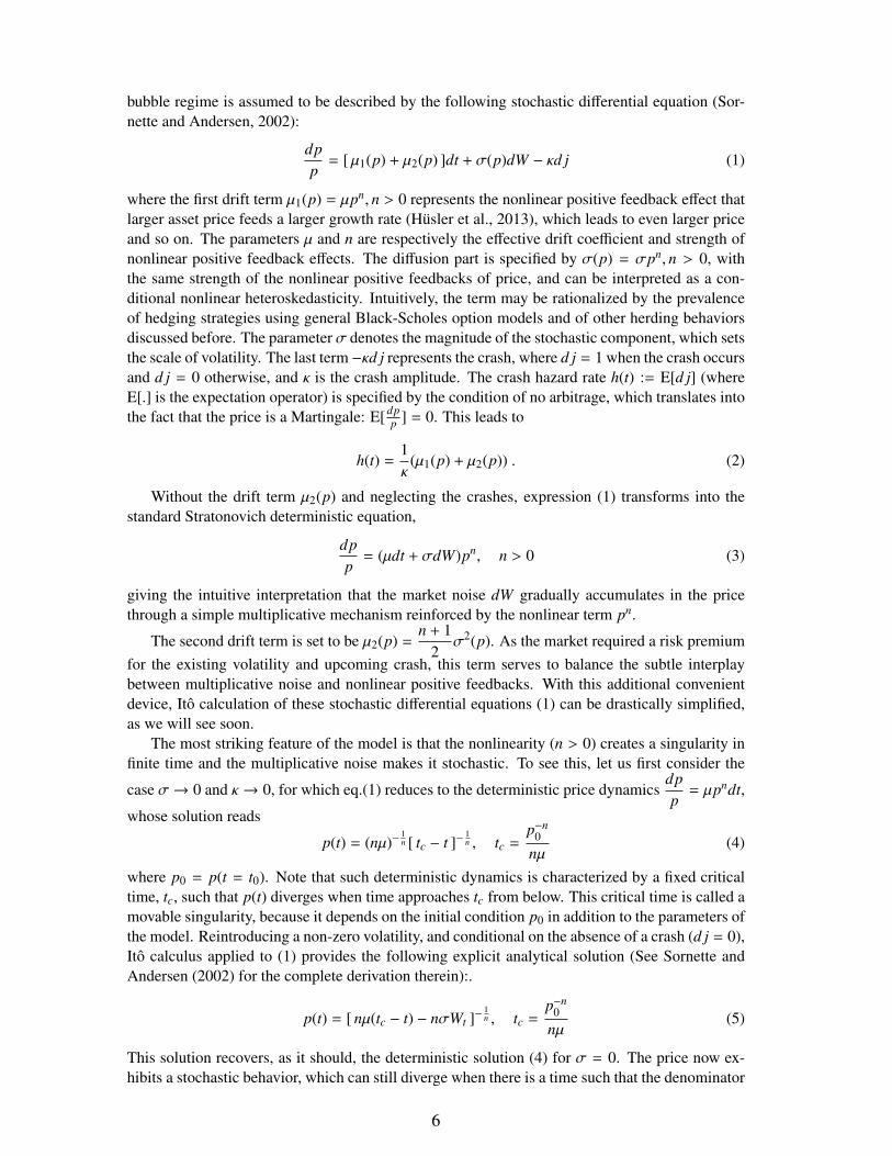
bubble regime is assumed to be described by the following stochastic differential equation (Sor-nette and Andersen, 2002):

dpp

= [ µ1(p) + µ2(p) ]dt + σ(p)dW − κd j (1)

where the first drift term µ1(p) = µpn, n > 0 represents the nonlinear positive feedback effect thatlarger asset price feeds a larger growth rate (Husler et al., 2013), which leads to even larger priceand so on. The parameters µ and n are respectively the effective drift coefficient and strength ofnonlinear positive feedback effects. The diffusion part is specified by σ(p) = σpn, n > 0, withthe same strength of the nonlinear positive feedbacks of price, and can be interpreted as a con-ditional nonlinear heteroskedasticity. Intuitively, the term may be rationalized by the prevalenceof hedging strategies using general Black-Scholes option models and of other herding behaviorsdiscussed before. The parameter σ denotes the magnitude of the stochastic component, which setsthe scale of volatility. The last term −κd j represents the crash, where d j = 1 when the crash occursand d j = 0 otherwise, and κ is the crash amplitude. The crash hazard rate h(t) := E[d j] (whereE[.] is the expectation operator) is specified by the condition of no arbitrage, which translates intothe fact that the price is a Martingale: E[ dp

p ] = 0. This leads to

h(t) =1κ

(µ1(p) + µ2(p)) . (2)

Without the drift term µ2(p) and neglecting the crashes, expression (1) transforms into thestandard Stratonovich deterministic equation,

dpp

= (µdt + σdW)pn, n > 0 (3)

giving the intuitive interpretation that the market noise dW gradually accumulates in the pricethrough a simple multiplicative mechanism reinforced by the nonlinear term pn.

The second drift term is set to be µ2(p) =n + 1

2σ2(p). As the market required a risk premium

for the existing volatility and upcoming crash, this term serves to balance the subtle interplaybetween multiplicative noise and nonlinear positive feedbacks. With this additional convenientdevice, Ito calculation of these stochastic differential equations (1) can be drastically simplified,as we will see soon.

The most striking feature of the model is that the nonlinearity (n > 0) creates a singularity infinite time and the multiplicative noise makes it stochastic. To see this, let us first consider the

case σ→ 0 and κ → 0, for which eq.(1) reduces to the deterministic price dynamicsdpp

= µpndt,

whose solution reads

p(t) = (nµ)−1n [ tc − t ]−

1n , tc =

p−n0

nµ(4)

where p0 = p(t = t0). Note that such deterministic dynamics is characterized by a fixed criticaltime, tc, such that p(t) diverges when time approaches tc from below. This critical time is called amovable singularity, because it depends on the initial condition p0 in addition to the parameters ofthe model. Reintroducing a non-zero volatility, and conditional on the absence of a crash (d j = 0),Ito calculus applied to (1) provides the following explicit analytical solution (See Sornette andAndersen (2002) for the complete derivation therein):.

p(t) = [ nµ(tc − t) − nσWt ]−1n , tc =

p−n0

nµ(5)

This solution recovers, as it should, the deterministic solution (4) for σ = 0. The price now ex-hibits a stochastic behavior, which can still diverge when there is a time such that the denominator

6

nµ(tc − t)− nσWt crosses 0. At t = 0, the denominator starts from an initial positive value nµtc. Inthe presence of the negative drift −nµt and notwithstanding the presence of the Wiener process,the denominator will cross 0 with probability 1. The corresponding stochastic critical time tc atwhich the price diverges is thus controlled by a first-passage problem when the drifting randomwalk motion nµt + nσWt first encounters the value nµtc = p−n

0 . From standard results of first-passage problems (Redner, 2001; Jeanblanc et al., 2009), the stochastic critical time tc is found tobe distributed according to the Inverse Gaussian distribution

tc ∼ IG

p−n0

nµ,

[ p−n0

nσ

]2 . (6)

In fact, with the specification (1) augmented by (2), the price never diverges. This is because,as the price accelerates, so does even more its instantaneous growth rate µ1(p)+µ2(p) and thereforeso does the crash hazard rate via expression (2). This is aimed at embodying the fact that thebubble collapses as a result of the ebb of speculation and withdrawal of intended demand when anunsustainable state is becoming more obvious or due to increasing scarcity of money and credit. Inother words, a crash always occurs before the price goes too high, ensuring long-term stationarity(Sornette and Andersen, 2002).

Note that the price dynamics (5) reduces to the geometric random walk when the strength ofpositive feedback vanishes (n = 0):

limn→0

p(t) = p0 · limn→0

[ 1 − n(µt + σWt) ]−1n = p0 e µt+σWt , (7)

which is indeed the solution of the standard Black-Scholes framework obtained as the limit n→ 0of equation (1) (with κ = 0).

2.2 Hidden Markov modelling (HMM) calibration approachWe propose to extend the Sornette-Andersen model summarized in the previous section by com-bining it with a standard geometric random walk, supposed to represent the normal regime ofmarkets. The complete price process is then described by regime switching between the dy-namics described by the Sornette-Andersen model with significantly positive value of n and thedegenerated geometric random walk for n = 0. Then, the existence of speculative trading can bejudged by estimating the probability that the market is in bubble state (n > 0) or in the normalstate (n = 0). For this, we convert the bubble model into a Hidden Markov modeling (HMM)framework and then calibrate all parameters in the model to identify the onsets and ends of bub-bles, following a procedure that we now describe. Because crashes represented by the jump termd j in (1) as rare, we chose to not identify them and only rely on the structural differences betweenthe process conditional on no crash for n > 0 and n = 0.

For the sake of conciseness and efficiency of the presentation, in the following discussion,we introduce a novel mathematical representation of probability distribution functions and ofconditional density functions. They resemble the famous “bra-ket” notations in Dirac notationsin Quantum Mechanics. To be clear, no new results are derived, it is just a notation used for itscompactness and coherence. The notations are as follows. We use “bra” to denote the probabilitydensity for a random variable, i.e., 〈 x | := fx(x); We use “ket” to denote the “conditional on”operation. Formal “multiplication” of a bra-vector and a ket vector gives the conditional density,i.e., 〈 x | · |y 〉 = 〈 x | y 〉 := fx|y(x|y). In the Appendix A, we show that, with the addition of afew formal transformation rules, more complicated expressions can be nicely represented, suchas the decomposed conditional joint density or Bayesian formulas for multivariate conditionaldensities. This is convenient to present the derivation of the formulas of our proposed HMM

7

procedure developed to estimate the super-exponential Sornette-Andersen bubble model from theperspective of a state-dependent regime-switching process.

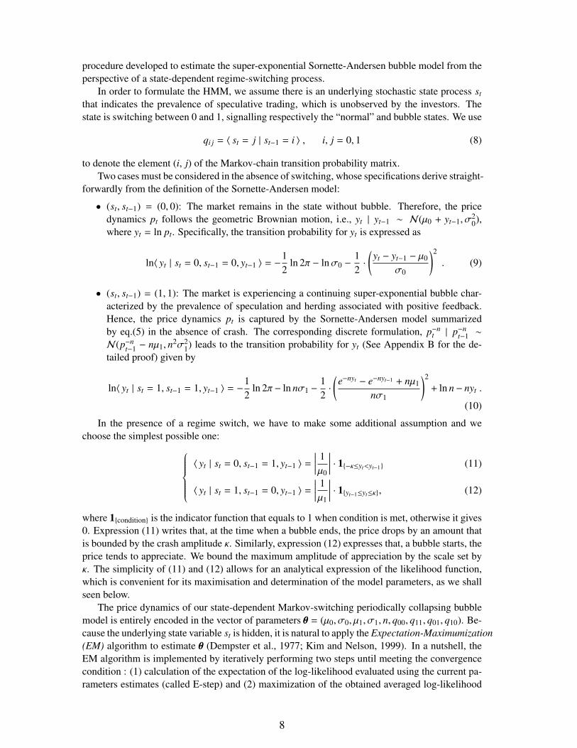
In order to formulate the HMM, we assume there is an underlying stochastic state process st

that indicates the prevalence of speculative trading, which is unobserved by the investors. Thestate is switching between 0 and 1, signalling respectively the “normal” and bubble states. We use

qi j = 〈 st = j | st−1 = i 〉 , i, j = 0, 1 (8)

to denote the element (i, j) of the Markov-chain transition probability matrix.Two cases must be considered in the absence of switching, whose specifications derive straight-

forwardly from the definition of the Sornette-Andersen model:

• (st, st−1) = (0, 0): The market remains in the state without bubble. Therefore, the pricedynamics pt follows the geometric Brownian motion, i.e., yt | yt−1 ∼ N(µ0 + yt−1, σ

20),

where yt = ln pt. Specifically, the transition probability for yt is expressed as

ln〈 yt | st = 0, st−1 = 0, yt−1 〉 = −12

ln 2π − lnσ0 −12·

(yt − yt−1 − µ0

σ0

)2

. (9)

• (st, st−1) = (1, 1): The market is experiencing a continuing super-exponential bubble char-acterized by the prevalence of speculation and herding associated with positive feedback.Hence, the price dynamics pt is captured by the Sornette-Andersen model summarizedby eq.(5) in the absence of crash. The corresponding discrete formulation, p−n

t | p−nt−1 ∼

N(p−nt−1 − nµ1, n2σ2

1) leads to the transition probability for yt (See Appendix B for the de-tailed proof) given by

ln〈 yt | st = 1, st−1 = 1, yt−1 〉 = −12

ln 2π− ln nσ1 −12·

(e−nyt − e−nyt−1 + nµ1

nσ1

)2

+ ln n− nyt .

(10)

In the presence of a regime switch, we have to make some additional assumption and wechoose the simplest possible one:

〈 yt | st = 0, st−1 = 1, yt−1 〉 =

∣∣∣∣∣ 1µ0

∣∣∣∣∣ · 1{−κ≤yt<yt−1} (11)

〈 yt | st = 1, st−1 = 0, yt−1 〉 =

∣∣∣∣∣ 1µ1

∣∣∣∣∣ · 1{yt−1≤yt≤κ}, (12)

where 1{condition} is the indicator function that equals to 1 when condition is met, otherwise it gives0. Expression (11) writes that, at the time when a bubble ends, the price drops by an amount thatis bounded by the crash amplitude κ. Similarly, expression (12) expresses that, a bubble starts, theprice tends to appreciate. We bound the maximum amplitude of appreciation by the scale set byκ. The simplicity of (11) and (12) allows for an analytical expression of the likelihood function,which is convenient for its maximisation and determination of the model parameters, as we shallseen below.

The price dynamics of our state-dependent Markov-switching periodically collapsing bubblemodel is entirely encoded in the vector of parameters θθθ = (µ0, σ0, µ1, σ1, n, q00, q11, q01, q10). Be-cause the underlying state variable st is hidden, it is natural to apply the Expectation-Maximumization(EM) algorithm to estimate θθθ (Dempster et al., 1977; Kim and Nelson, 1999). In a nutshell, theEM algorithm is implemented by iteratively performing two steps until meeting the convergencecondition : (1) calculation of the expectation of the log-likelihood evaluated using the current pa-rameters estimates (called E-step) and (2) maximization of the obtained averaged log-likelihood

8

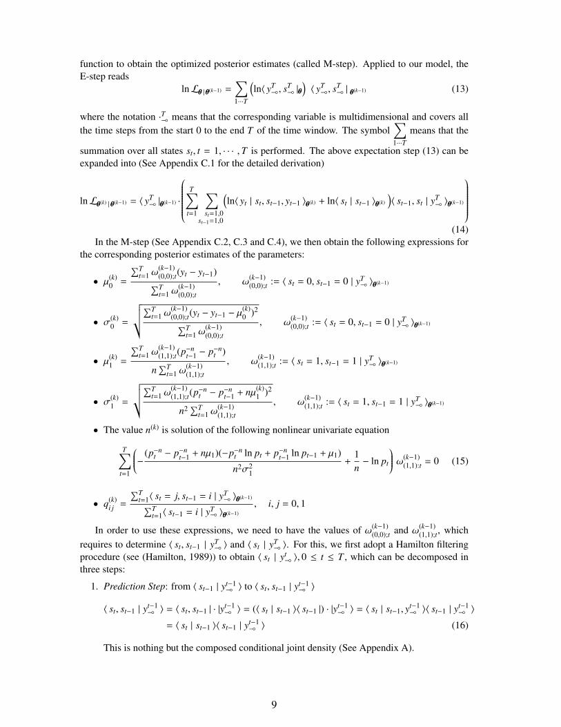
function to obtain the optimized posterior estimates (called M-step). Applied to our model, theE-step reads

lnLθθθ |θθθ(k−1) =∑1···T

(ln〈 yT

(, sT( |θθθ

)〈 yT(, s

T( | θθθ(k−1) (13)

where the notation ·T( means that the corresponding variable is multidimensional and covers allthe time steps from the start 0 to the end T of the time window. The symbol

∑1···T

means that the

summation over all states st, t = 1, · · · ,T is performed. The above expectation step (13) can beexpanded into (See Appendix C.1 for the detailed derivation)

lnLθθθ(k) |θθθ(k−1) = 〈 yT( |θθθ(k−1) ·

T∑

t=1

∑st=1,0

st−1=1,0

(ln〈 yt | st, st−1, yt−1 〉θθθ(k) + ln〈 st | st−1 〉θθθ(k)

)〈 st−1, st | yT

( 〉θθθ(k−1)

(14)

In the M-step (See Appendix C.2, C.3 and C.4), we then obtain the following expressions forthe corresponding posterior estimates of the parameters:

• µ(k)0 =

∑Tt=1 ω

(k−1)(0,0);t(yt − yt−1)∑Tt=1 ω

(k−1)(0,0);t

, ω(k−1)(0,0);t := 〈 st = 0, st−1 = 0 | yT

( 〉θθθ(k−1)

• σ(k)0 =

√√√∑Tt=1 ω

(k−1)(0,0);t(yt − yt−1 − µ

(k)0 )2∑T

t=1 ω(k−1)(0,0);t

, ω(k−1)(0,0);t := 〈 st = 0, st−1 = 0 | yT

( 〉θθθ(k−1)

• µ(k)1 =

∑Tt=1 ω

(k−1)(1,1);t(p−n

t−1 − p−nt )

n∑T

t=1 ω(k−1)(1,1);t

, ω(k−1)(1,1);t := 〈 st = 1, st−1 = 1 | yT

( 〉θθθ(k−1)

• σ(k)1 =

√√√∑Tt=1 ω

(k−1)(1,1);t(p−n

t − p−nt−1 + nµ(k)

1 )2

n2 ∑Tt=1 ω

(k−1)(1,1);t

, ω(k−1)(1,1);t := 〈 st = 1, st−1 = 1 | yT

( 〉θθθ(k−1)

• The value n(k) is solution of the following nonlinear univariate equation

T∑t=1

− (p−nt − p−n

t−1 + nµ1)(−p−nt ln pt + p−n

t−1 ln pt−1 + µ1)

n2σ21

+1n− ln pt

ω(k−1)(1,1):t = 0 (15)

• q(k)i j =

∑Tt=1〈 st = j, st−1 = i | yT

( 〉θθθ(k−1)∑Tt=1〈 st−1 = i | yT

( 〉θθθ(k−1)

, i, j = 0, 1

In order to use these expressions, we need to have the values of ω(k−1)(0,0);t and ω(k−1)

(1,1);t, whichrequires to determine 〈 st, st−1 | yT

( 〉 and 〈 st | yT( 〉. For this, we first adopt a Hamilton filtering

procedure (see (Hamilton, 1989)) to obtain 〈 st | yt( 〉, 0 ≤ t ≤ T , which can be decomposed in

three steps:

1. Prediction Step: from 〈 st−1 | yt−1( 〉 to 〈 st, st−1 | yt−1

( 〉

〈 st, st−1 | yt−1( 〉 = 〈 st, st−1 | · |yt−1

( 〉 = (〈 st | st−1 〉〈 st−1 |) · |yt−1( 〉 = 〈 st | st−1, yt−1

( 〉〈 st−1 | yt−1( 〉

= 〈 st | st−1 〉〈 st−1 | yt−1( 〉 (16)

This is nothing but the composed conditional joint density (See Appendix A).

9

2. Updating Step: from 〈 st, st−1 | yt−1( 〉 to 〈 st, st−1 | yt

( 〉

〈 st, st−1 | yt( 〉 = 〈 st, st−1 | yt−1

( , yt 〉 = 〈 st, st−1 | yt−1( 〉〈 yt | st, st−1, yt−1

( 〉

〈 yt | yt−1( 〉

(17)

=〈 yt | st, st−1, yt−1

( 〉〈 st, st−1 | yt−1( 〉∑

t−1,t〈 yt | st, st−1, yt−1( 〉〈 st, st−1 | yt−1

( 〉(18)

The validity of eq. (17) is based on the multivariate Bayesian formula (See Appendix A fordetails).

3. Summation Step: from 〈 st, st−1 | yt( 〉 to 〈 st | yt

( 〉

〈 st | yt( 〉 = 〈 st | ·

∑t−1

|st−1 〉〈 st−1 |

|yt( 〉 =

∑t−1

〈 st | st−1 〉〈 st−1 |

|yt( 〉 =

∑t−1

〈 st, st−1 |

|yt( 〉

=∑t−1

〈 st, st−1 | yt( 〉 (19)

This provides the filtering probability 〈 st | yt( 〉, which quantifies the probability for a given

bubble state to be present, based on the current available market information.

Second, with the obtained filtering probability, we take advantage of a backward smoothingapproach to estimate 〈 st, st−1 | yT

( 〉 and 〈 st | yT( 〉, which is inspired by Kim’s smoothing routine

(See Kim and Nelson (1999) for a discussion therein). Let y(t+1 denote all of the remaining log-prices ln(pt) expressed at time following time t in the observation window from 1 to T , i.e.,yT( = {yt

(, y(t+1}. The backward prediction is then expressed as

〈 st+1, st | yT( 〉 = 〈 st | st+1, yT

( 〉〈 st+1 | yT( 〉 = 〈 st | st+1, yt

(, y(t+1 〉〈 st+1 | yT

( 〉 (20)

= 〈 st | st+1, yt( 〉〈 st+1 | yT

( 〉 = 〈 st | yt( 〉〈 st+1 | st, yt

( 〉

〈 st+1 | yt( 〉

〈 st+1 | yT( 〉 (21)

= 〈 st | yt( 〉〈 st+1 | yT

( 〉〈 st+1 | st 〉∑

t〈 st+1 | st 〉〈 st | yt( 〉

. (22)

The derivation of the r.h.s. in (21) is based on the multivariate Bayesian formula (See AppendixA). The detailed derivation from (20) to (21) can be found in Appendix C.5. This finally leads tothe following expression to calculate 〈 st | yT

( 〉, which can be called smoothing probability:

〈 st | yT( 〉 =

∑t+1

〈 st | st+1 〉〈 st+1 | yT( 〉 =

∑t+1

〈 st+1, st | yT( 〉, t = 1, · · · ,T − 1 . (23)

As its mathematical denotation to indicate, the smoothing probability 〈 st | yT( 〉 measures the

likelihood of the existence of bubbles in a given time interval by including the information offuture prices. For our purpose of diagnosing a bubble and its possible dangerous time period fora burst, it is necessary to use the causal filtering probability 〈 st | yt

( 〉 and not the non-causalsmoothing probability 〈 st | yT

( 〉. The later can however be useful for parameter estimations,which themselves impact on bubble detection.

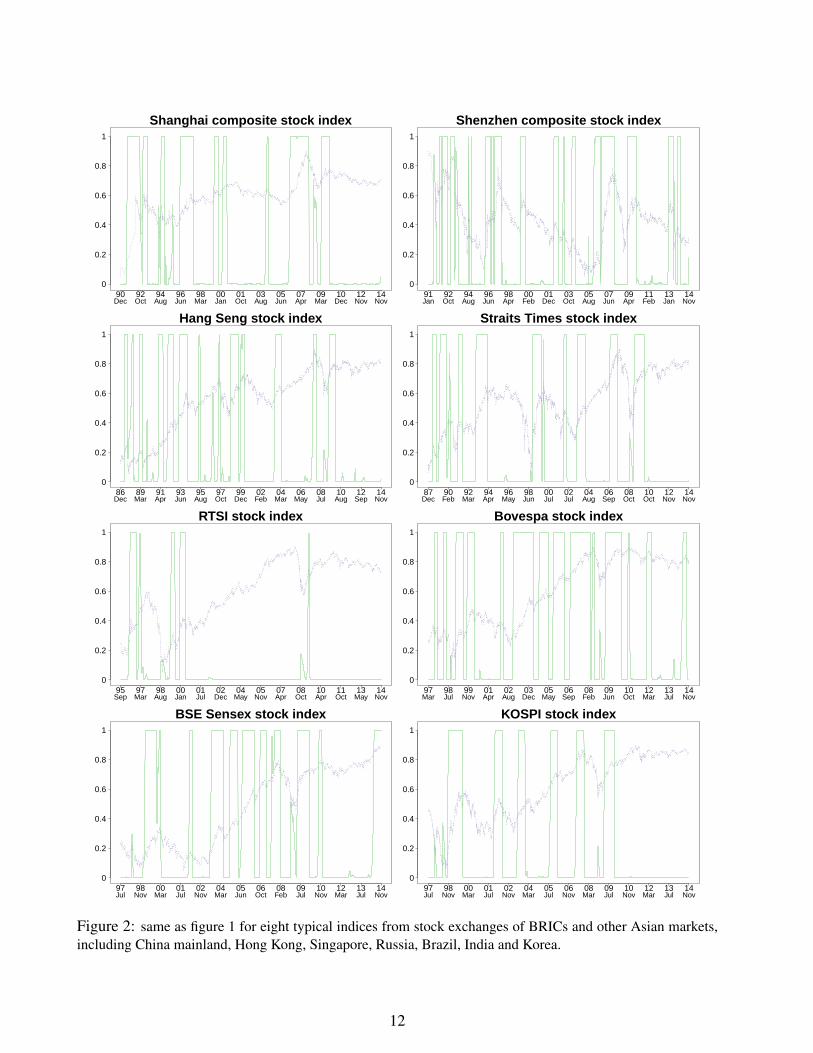
2.3 Empirical estimation of the bubble probability in 16 financialmarketsFigs. 1 and 2 show the estimated daily smoothing probability for the presence of super-explosivebubbles based on the HMM procedure in sixteen different global financial markets, representedby their major stock indices. Correspondingly, Figs. 3 and 4 display the estimated daily filtering

10

0

0.2

0.4

0.6

0.8

1

80 82 85 88 90 93 96 98 01 04 06 09 12 14Jan Sep May Jan Sep May Jan Sep Jun Feb Oct Jul Mar Nov

NASDAQ stock index

0

0.2

0.4

0.6

0.8

1

80 82 85 88 90 93 96 98 01 04 06 09 12 14Jan Sep May Jan Sep May Jan Sep Jun Feb Oct Jul Mar Nov

S&P 500 stock index

0

0.2

0.4

0.6

0.8

1

84 86 88 91 93 95 98 00 02 05 07 10 12 14Jan May Sep Feb Jun Nov Mar Aug Dec May Sep Feb Jun Nov

FTSE 100 stock index

0

0.2

0.4

0.6

0.8

1

84 86 88 91 93 95 98 00 02 05 07 10 12 14Jan May Oct Feb Jul Nov Mar Aug Dec May Oct Feb Jul Nov

Nikkei stock index

0

0.2

0.4

0.6

0.8

1

90 92 94 95 97 99 01 03 05 07 09 11 12 14Mar Feb Jan Dec Nov Oct Sep Aug Jun May Mar Feb Dec Nov

CAC40 stock index

0

0.2

0.4

0.6

0.8

1

90 92 94 96 98 00 02 03 05 07 09 11 13 14Nov Oct Aug Jul May Mar Jan Nov Sep Jul May Mar Jan Nov

DAX stock index

0

0.2

0.4

0.6

0.8

1

97 99 00 01 03 04 05 07 08 09 10 12 13 14Dec Apr Aug Nov Mar Jun Oct Jan May Aug Dec Mar Jul Nov

FTSE MIB stock index

0

0.2

0.4

0.6

0.8

1

90 92 94 96 98 00 02 03 05 07 09 11 13 14Nov Sep Aug Jun Apr Feb Jan Nov Sep Jul Jun Mar Jan Nov

Swiss Market stock index

Figure 1: Estimated daily smoothing probabilities 〈 st | yT( 〉 of the periodical collapsing super-exponential

growth bubble embedded in the Hidden Markov Modeling (HMM) procedure represented with the palegreenthin continuous curve bouncing between 0 and 1 for eight stock exchanges: U.S. (Nasdaq and S&P500),U.K., Japan, France, Germany, Italy and Switzerland. All indices are given in logarithmic scale and arerescaled into [0,1] for comparison. In order to mitigate the effects of identifying regime-shift too of-ten as a result of daily price volatility, all indices are geometrically averaged over 100 days according toln pfiltered

t = (1/100)∑99

i=0 ln pt−i, before implementing the EM algorithm.11

0

0.2

0.4

0.6

0.8

1

90 92 94 96 98 00 01 03 05 07 09 10 12 14Dec Oct Aug Jun Mar Jan Oct Aug Jun Apr Mar Dec Nov Nov

Shanghai composite stock index

0

0.2

0.4

0.6

0.8

1

91 92 94 96 98 00 01 03 05 07 09 11 13 14Jan Oct Aug Jun Apr Feb Dec Oct Aug Jun Apr Feb Jan Nov

Shenzhen composite stock index

0

0.2

0.4

0.6

0.8

1

86 89 91 93 95 97 99 02 04 06 08 10 12 14Dec Mar Apr Jun Aug Oct Dec Feb Mar May Jul Aug Sep Nov

Hang Seng stock index

0

0.2

0.4

0.6

0.8

1

87 90 92 94 96 98 00 02 04 06 08 10 12 14Dec Feb Mar Apr May Jun Jul Jul Aug Sep Oct Oct Nov Nov

Straits Times stock index

0

0.2

0.4

0.6

0.8

1

95 97 98 00 01 02 04 05 07 08 10 11 13 14Sep Mar Aug Jan Jul Dec May Nov Apr Oct Apr Oct May Nov

RTSI stock index

0

0.2

0.4

0.6

0.8

1

97 98 99 01 02 03 05 06 08 09 10 12 13 14Mar Jul Nov Apr Aug Dec May Sep Feb Jun Oct Mar Jul Nov

Bovespa stock index

0

0.2

0.4

0.6

0.8

1

97 98 00 01 02 04 05 06 08 09 10 12 13 14Jul Nov Mar Jul Nov Mar Jun Oct Feb Jul Nov Mar Jul Nov

BSE Sensex stock index

0

0.2

0.4

0.6

0.8

1

97 98 00 01 02 04 05 06 08 09 10 12 13 14Jul Nov Mar Jul Nov Mar Jul Nov Mar Jul Nov Mar Jul Nov

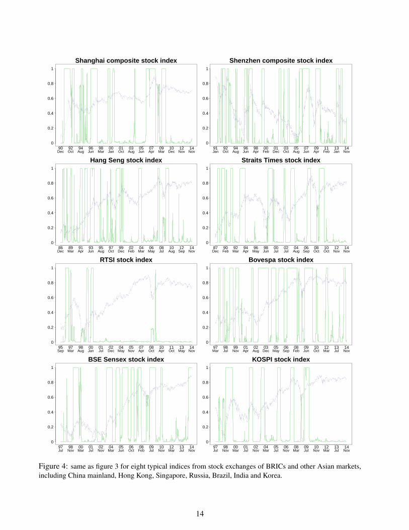
KOSPI stock index

Figure 2: same as figure 1 for eight typical indices from stock exchanges of BRICs and other Asian markets,including China mainland, Hong Kong, Singapore, Russia, Brazil, India and Korea.

12

0

0.2

0.4

0.6

0.8

1

80 82 85 88 90 93 96 98 01 04 06 09 12 14Jan Sep May Jan Sep May Jan Sep Jun Feb Oct Jul Mar Nov

NASDAQ stock index

0

0.2

0.4

0.6

0.8

1

80 82 85 88 90 93 96 98 01 04 06 09 12 14Jan Sep May Jan Sep May Jan Sep Jun Feb Oct Jul Mar Nov

S&P 500 stock index

0

0.2

0.4

0.6

0.8

1

84 86 88 91 93 95 98 00 02 05 07 10 12 14Jan May Sep Feb Jun Nov Mar Aug Dec May Sep Feb Jun Nov

FTSE 100 stock index

0

0.2

0.4

0.6

0.8

1

84 86 88 91 93 95 98 00 02 05 07 10 12 14Jan May Oct Feb Jul Nov Mar Aug Dec May Oct Feb Jul Nov

Nikkei stock index

0

0.2

0.4

0.6

0.8

1

90 92 94 95 97 99 01 03 05 07 09 11 12 14Mar Feb Jan Dec Nov Oct Sep Aug Jun May Mar Feb Dec Nov

CAC40 stock index

0

0.2

0.4

0.6

0.8

1

90 92 94 96 98 00 02 03 05 07 09 11 13 14Nov Oct Aug Jul May Mar Jan Nov Sep Jul May Mar Jan Nov

DAX stock index

0

0.2

0.4

0.6

0.8

1

97 99 00 01 03 04 05 07 08 09 10 12 13 14Dec Apr Aug Nov Mar Jun Oct Jan May Aug Dec Mar Jul Nov

FTSE MIB stock index

0

0.2

0.4

0.6

0.8

1

90 92 94 96 98 00 02 03 05 07 09 11 13 14Nov Sep Aug Jun Apr Feb Jan Nov Sep Jul Jun Mar Jan Nov

Swiss Market stock index

Figure 3: Estimated daily filtering probabilities 〈 st | yt( 〉 of the periodical collapsing super-exponential growth

bubble embedded in the Hidden Markov Modeling (HMM) procedure represented with the palegreen thin con-tinuous curve bouncing between 0 and 1 for eight stock exchanges: U.S. (Nasdaq and S&P500), U.K., Japan,France, Germany, Italy and Switzerland. All indices are given in logarithmic scale and are rescaled into [0,1]for comparison. In order to mitigate the effects of identifying regime-shift too often as a result of daily pricevolatility, all indices are geometrically averaged over 100 days according to ln pfiltered

t = (1/100)∑99

i=0 ln pt−i,before implementing the EM algorithm.

13

0

0.2

0.4

0.6

0.8

1

90 92 94 96 98 00 01 03 05 07 09 10 12 14Dec Oct Aug Jun Mar Jan Oct Aug Jun Apr Mar Dec Nov Nov

Shanghai composite stock index

0

0.2

0.4

0.6

0.8

1

91 92 94 96 98 00 01 03 05 07 09 11 13 14Jan Oct Aug Jun Apr Feb Dec Oct Aug Jun Apr Feb Jan Nov

Shenzhen composite stock index

0

0.2

0.4

0.6

0.8

1

86 89 91 93 95 97 99 02 04 06 08 10 12 14Dec Mar Apr Jun Aug Oct Dec Feb Mar May Jul Aug Sep Nov

Hang Seng stock index

0

0.2

0.4

0.6

0.8

1

87 90 92 94 96 98 00 02 04 06 08 10 12 14Dec Feb Mar Apr May Jun Jul Jul Aug Sep Oct Oct Nov Nov

Straits Times stock index

0

0.2

0.4

0.6

0.8

1

95 97 98 00 01 02 04 05 07 08 10 11 13 14Sep Mar Aug Jan Jul Dec May Nov Apr Oct Apr Oct May Nov

RTSI stock index

0

0.2

0.4

0.6

0.8

1

97 98 99 01 02 03 05 06 08 09 10 12 13 14Mar Jul Nov Apr Aug Dec May Sep Feb Jun Oct Mar Jul Nov

Bovespa stock index

0

0.2

0.4

0.6

0.8

1

97 98 00 01 02 04 05 06 08 09 10 12 13 14Jul Nov Mar Jul Nov Mar Jun Oct Feb Jul Nov Mar Jul Nov

BSE Sensex stock index

0

0.2

0.4

0.6

0.8

1

97 98 00 01 02 04 05 06 08 09 10 12 13 14Jul Nov Mar Jul Nov Mar Jul Nov Mar Jul Nov Mar Jul Nov

KOSPI stock index

Figure 4: same as figure 3 for eight typical indices from stock exchanges of BRICs and other Asian markets,including China mainland, Hong Kong, Singapore, Russia, Brazil, India and Korea.

14

probability for the presence of super-explosive bubbles for the same sixteen global financial mar-kets. The studied stock indices include the US NASDAQ index and S&P 500 stock index from theNew York Stock Exchange, the FTSE 100 index from London Stock Exchange, the Nikkei 225index from Tokyo Stock Exchange, the CAC40 stock index from Euronext Paris, the DAX indexfrom Frankfurt Stock Exchange in Germany, Switzerland’s blue-chip stock market index (SMI),the FTSE MIB stock index from Borsa Italiana, the two major stock indices from Chinese stockmarket (Shanghai composite index and Shenzhen composite index), the Hang Seng index fromHong Kong Stock Exchange, the Straits Times stock index from Singapore Exchange, the Rus-sia Trading System (RTS) index from Moscow Stock Echange, the Bovespa index from the SaoPaulo Stock, Mercantile & Futures Exchange, the SENSEX index from Bombay Stock Exchangein India and the Korea Composite Stock Price Index(KOSPI). In the implementation of our EMprocedure, the condition of convergence of the algorithm is specified as

∆ =lnLθθθ(k+1) |θθθ(k) − lnLθθθ(k) |θθθ(k−1)

lnL′θθθ(k) |θθθ(k−1)≤ 0.0001 (24)

Several observations are worth describing.• There is an excellent correspondence between the estimated daily smoothing and filtering

probabilities in essentially all cases: the periods identified in the super-exponential bubble statewith the smoothing probability 〈 st | yT

( 〉 using the information contained in the complete timeseries match remarkably closely those intervals identified in the super-exponential bubble statewith the causal filtering probability 〈 st | yt

( 〉 that use data up to the running present time t. Thisis perhaps not too surprising since our bubble detection method does not rely on the existenceof a crash or change of regime but solely on the identification of a transient super-exponentialdynamics.• It is quite striking that the periods identified in the super-exponential bubble state are in

general associated with a strong upward price dynamics (not a surprise from the constructionof the model) ending with a peak of the price followed by a clear change of price regime (thissecond property being much less trivial). This change can take the form of a significant correctionor crash, of a sideway volatile dynamics or of a downward price momentum. The presence ofsuch changes of regime is a pleasant qualitative confirmation of one of the key insights of super-exponential models, namely the non-sustainable nature of the price dynamics that has to breakinto a slower growth, in fact often a reversal.• While most bubble researchers would agree on the diagnostic of a bubble in a number of

cases found to correspond to large values of our smoothing and filtering probabilities, such asduring the price ascent associated with the dot-com bubble in Western markets, which is herecorrectly identified by our method, one could raise the criticism that many periods are pickedout that do not correspond to the times of well-documented bubbles, raising the spectrum oftoo many false alarms (false positives or errors of type I). In response to this, we argue that, assaid above, most of these identified bubble periods are followed by a significant change of priceregime, which can be taken as a validation of the bubble identification. Moreover, it is the goalof a better model with superior implementation to indeed reveal hitherto hidden aspects of theprice dynamics. Thus, it should not be a surprise that our method identifies a number of bubbleregimes that would have not been suspected by other means. Figs. 1-4 thus lead us to conjecturethat financial markets are much more often in bubble states that previous believed.

We have quantified the fractions of time, weighted by the corresponding probabilities, that the16 studied markets are in a bubble. Table1 below lists the results, with the fractions expressedas percentages. The notations p.b(filter) and p.b(smoothing) indicate the fractions of time whenmarkets are in a bubble regime, as determined respectively by filtering probabilities and smoothingprobabilities. These fractions are obtained as the integral of the corresponding probabilities shownin Fig. 1 - 4 over the whole time period for each of the 16 investigated markets. Except for the

15

Russian market with fractions as low as 8%, the chance for western stock markets to be in bubbleregime is typically in the range 10%-15% cross-sectionally. In contrast, emerging markets as wellas Japan market, the only developed market in Asia, are found about 20% to 45% of the timein the bubble regime. This may due to the less transparent information environment as well asweaker regulatory control, which tends to promote herding.

Table 1: Fractions of time that the sixteen studied stock markets are in bubble regime. We give thefractions with only two digits, as a higher precision would be provide a misleading sense of accuracy.

Stock Index p.b(filter,%) p.b(smoothing,%)

NASDAQ 15 16SP500 12 12FTSE 10 11RTSI 8 9

CAC40 12 13DAX 11 11MIB 12 13SMI 12 13N225 40 43SSEC 30 30SZSC 32 32HSI 24 25STI 27 28

BVSP 46 46SENSEX 36 38

KS11 23 23

• The previous remark raised the issue of false positives. What about false negatives or errorsof type II? Some studies have suggested that the run-ups of stock market prices of Western mar-kets from 2003 to 2007 qualify as a bubble (Sornette and Woodard, 2010; Sornette and Cauwels,2014, 2015). In contrast, Figs. 1 and Fig. 3 give a zero bubble probability for this time interval forall Western markets. One likely explanation of these missed targets was advanced by Andersenand Sornette (2004), who stressed that, by construction the (Sornette and Andersen, 2002) modelassumes that bubbles are associated to both a super-exponential price appreciation and a corre-sponding explosion of the volatility. But Andersen and Sornette (2004) showed that, for a numberof historical bubbles, this is counterfactual: many bubbles develop without a clear increase ofvolatility, which would then lead the Sornette-Andersen model to be rejected. Indeed, many bub-bles are developing over a time of complacent view of the underlying risks, in other words, thegenuine risks are under-estimated and the crash often comes as a surprise. This led Andersenand Sornette (2004) to suggest the existence of at least two types of bubbles, the “fearful” (resp.“fearless”) bubbles associated with an increasing (resp. constant or decreasing) volatility. Ourpresent investigation can thus be understood as targeting only the fearful bubbles.

3 Speculative Influence Network

3.1 DefinitionsWe introduce the Speculative Influence Network (SIN) as a directional weighted network of fi-nancial assets, such as stocks, bonds, mutual funds, real estate, forex, commodities, derivatives

16

and so on, which is organized to map the mutual relationships representing the speculative influ-ences between them, i.e., how speculative trading of one asset may draw speculative trading inanother assets. The arrow of a link in the SIN then indicates the direction of the speculative trad-ing influence, and its weight quantifies the intensity of the influence. In order to derive the causalspeculative influence between assets, we propose a two-steps procedure: (i) estimate for each assetthe daily filtering probability for the presence of super-explosive bubbles using the HMM basedapproach developed in Section 2.2 with the regime-switching Sornette-Andersen bubble model;(ii) once two assets are diagnosed as being in a bubble state, identify the possible causal flow ofthe probabilities from one asset to the other in order to infer a possible influence or contagioneffect. In other words, provided one asset X is diagnosed to be in a bubble, we want to estimatehow much does it influences the probability of another asset Y to be also in the bubble state.

There are at least two well-known methods to detect causal relationship between time-series,the Granger Causality test and the information-based Transfer Entropy (TE) formulation. Theformer is relatively “cheaper”, being linear by construction, while the later encompasses nonlinearrelationship and does not rely on a model specification. Although the Granger Causality test ismore popular in economics and finance, it is mainly designed for multivariate linear autoregressiveprocesses with white-noise residuals. For general nonlinear stochastic time series, it provides onlyan approximate measure of causal influence (Barrett and Barnett, 2013). Moreover, elegant proofsshow that the two methods are only equivalent for Gaussian, exponential Weinman and log-normalvariables (Barnett et al., 2009; Hlavackova-Schindler, 2011). Our inputs are the time series of thefiltering probabilities 〈 st | yt

( 〉 for all assets, which exhibit properties far from the conditionsof application of the Granger Causality test: (i) the 〈 st | yt

( 〉’s are bounded in [0, 1]; (ii) theyexhibit strong non-Gaussian characteristics with a pronounced bimodality near 0 or 1; there is noguarantee that they obey autoregressive processes. Therefore, we prefer to use the TE method inthe remaining of the article.

3.2 Transfer EntropyIn his famous work “A Mathematical Theory of Communication”, Shannon pioneered a novelmetric to quantify the uncertainty of an outcome from a set of possible events, the so-called Shan-non Entropy. In order to capture the average uncertainty in a system that is comprised of a set ofevents with occurrence probabilities pi, i = 1, · · · , n, the Shannon Entropy (SE) H(p1, p2, · · · , pn)is required to satisfy the following three properties:

1. H(p1, · · · , pn) should be continuous in pi.

2. If pi =1n, i = 1, · · · , n, then H(p1, · · · , pn) should monotonically increase with n.

3. If an event i can be further broken down into several sub-events, then the SE is updated byadding the sums of the SE of such event with weights equal to their occurrence probabilities,i.e., Hnew = Hold + piHi, where Hi is the value of the function H for the composite event.

Then, it can be proved that these three properties lead to the unique Shannon Entropy function

H = −

N∑i=1

pi logs pi = −

N∑i=1

〈 i | logs〈 i |, where the base s of the logarithm is arbitrary and depends

on the chosen information units. For example, s is often selected to be equal to 2 when the measureis given in terms of bits of information. Shannon Entropy bears a lot of resemblance to Gibbs’entropy, which quantifies the degree of diversity for a system’s possible micro-states. But SE ismore general and gauges the necessary external information inflow needed to ascertain a specificmicro-state for a event to happen.

When dealing with systems that interact with each other, the notion of Transfer Entropy (TE)can be introduced to describe the extent to which the uncertainty of one system is influenced

17

by other systems inter-temporally. Consider two systems U and V that are Markov processes ofdegree kU and kV respectively. Let us denote the sets of possible events for U and V at time t byut and vt. Then, the TE from system V to U at time t is defined as

TEV→U(t) = −∑

ut ,··· ,ut−kUvt−1,··· ,vt−kV

〈 ut, · · · , ut−kU , vt−1, · · · , vt−kV | · logs〈 ut | ut−1, · · · , ut−kU 〉

−

−∑

ut ,··· ,ut−kUvt−1,··· ,vt−kV

〈 ut, · · · , ut−kU , vt−1, · · · , vt−kV | · logs〈 ut | ut−1, · · · , ut−kU , vt−1, · · · , vt−kV 〉

=

∑ut ,··· ,ut−kU

vt−1,··· ,vt−kV

〈 ut, · · · , ut−kU , vt−1, · · · , vt−kV | · logs〈 ut | ut−1, · · · , ut−kU , vt−1, · · · , vt−kV 〉

〈 ut | ut−1, · · · , ut−kU 〉

(25)

According to the above definition, the TE from V to U is just the difference between theamount of uncertainty for U when merely measured based on its past information and its amountof uncertainty when also taking account of V’s past information. Hence, the TE effectively mea-sures the reduction of uncertainty of system U achieved by using the information of system V . Inother words, it provides an evaluation of the power of V to predict the motion of U. It quantifiesthe strength of the causal relationship between U and V . In the following subsection, we showhow to use the TE to develop the SIN for financial markets.

3.3 Constructing the Speculative Influence Network (SIN) for a finan-cial marketIn the present work, the speculative influence relationship between two different financial assetsis measured by calculating the TE between the time-series of the filtering probabilities defined insubsection 2.2 and illustrated in subsection 2.3, conditional on the two assets being in the bubblestate. For this, we introduce the speculative influence intensity (SII) from X to Y as

S IIX→Y (t) = T Ep fb (X)→p f

b (Y)(t) , (26)

where the time-series p fb(X) =

{〈 st = 1 | ln pX,t, ln pX,t−1, · · · , ln pX,0 〉

}t=Tt=0 =

{〈 st = 1 | xt

( 〉}t=Tt=0

and p fb(Y) =

{〈 st = 1 | ln pY,t, ln pY,t−1, · · · , ln pY,0 〉

}t=Tt=0 =

{〈 st | yt

( 〉}t=Tt=0 respectively denote the

estimated filtering probability of staying in the bubble state for assets X and Y .According to the derivations presented in subsection 2.2, the filtering probability 〈 st | yt

( 〉 attime t only depends on the previous one 〈 st−1 | yt−1

( 〉 at t− 1 and on yt. This is intended to capturethe idea that the level of herding at a given time is mostly influenced by that of the previous timeperiod (day in our empirical estimations). Using this property, formula (25) for the TE of V to Ucan be simplified into

TEV→U(t) =∑

ut ,ut−1,vt−1

〈 ut, ut−1, vt−1 | · logs〈 ut | ut−1, vt−1 〉

〈 ut | ut−1 〉

=∑

ut ,ut−1,vt−1

〈 ut, ut−1, vt−1 | · logs〈 ut, ut−1, vt−1 |〈 ut−1 |

〈 ut, ut−1 |〈 ut−1, vt−1 |(27)

where U and V actually represent p fb(X) and p f

b(Y), and correspondingly ut = 〈 st = 1 | xt( 〉 and

vt = 〈 st = 1 | yt( 〉.

18

In order to use (27), we need to specify 〈 ut−1 |, 〈 ut−1, vt−1 |, 〈 ut, ut−1 | and 〈 ut, ut−1, vt−1 |. Forthis, we divide the range [0, 1] of p f

b(X) and p fb(Y) in 10 bins of equal width and treat each bin

as a unique identified event for gauging the presence of speculative herding. This coarse-grainingprocedure amounts to considering two events within a given bin as being undistinguishable and isperformed to reduce the sensitivity to noise and minimize the impact of model mis-specification.Correspondingly, the base s in (27) is set to 10 for the practical computing. Then, by countingthe number of different combinations associated with the value vector of time-series U up to acertain day, with the vector for U’s values lagged by one day and with the vector for V’s valuesalso lagged by one day, all four distributions 〈 ut−1 |, 〈 ut−1, vt−1 |, 〈 ut, ut−1 | and 〈 ut, ut−1, vt−1 | canbe empirically calculated. 〈 ut−1 | is obtained by taking the ratio of the number of times a 〈 ut−1 |

in a given bin appeared in the vector U by the total number of occurrences for all bins types.In order to estimate 〈 ut−1, vt−1 |, one must count how many times a particular combination ofbins, that the couple states (u, v) belongs to, appeared in the joint vector of lagged U’s valuesand lagged V’s values, and then normalise by the total number of occurrences for the pairs. Thecalculation of 〈 ut, ut−1, vt−1 | is similar to that of 〈 ut−1, vt−1 |, except that the counting is conductedon bins triplets that appear in the vector obtained by joining all three vectors. The calculation ofSII between arbitrary pairs of two investment targets finally gives the SII matrix for the wholefinancial market, which is the basic encoding scheme to derive the adjacency matrix that definesthe SIN.

The assets of interest are the nodes of the SIN. A relationship in which node Xi influencesnode X j is quantified by SIIXi→X j and is represented by a directed link Xi → X j. This doesnot exclude the possible existence of a direct influence in the opposite direction from node X j

to node Xi measured by SIIX j→Xi , making the SIN a bilateral directional network. In practice,we use a threshold so that values of SIIXi→X j below this threshold are considered too small tobe of significance and only the transfer entropies larger than this threshold will be used in theSIN representation. To further extract the leading influence relationship, we introduce the netspeculative influence intensity (NSII)

NSII Xi→X j(t) = SIIXi→X j(t) − SIIX j→Xi(t) , (28)

allowing us to reduce SIN to an unidirectional network capturing the net influence effects betweenassets. In this reduced unidirectional SIN, only positive NSII values need to be considered andare represented as arrows going from the influencer i to the receiver j (for NSII Xi→X j(t) > 0).

4 Early warnings of bubbles for Chinese Markets via SIN

4.1 Data and methodologyWe now investigate empirically how the Speculative Influence Network (SIN) can help provideeffective early warning signals by dissecting a bubble structure via a disaggregated firm levelanalysis. We show below that the SIN complements the more conventional bubble detectionmethod based on super-exponential growth signatures of the aggregated market, by providingindicators of strong speculative influence (or contagion) that can be useful by playing the roleof systemic risk gauges. Our tests consist in quantifying the out-of-sample performance of theprediction of the maximum cumulative lost proportion (%MaxLoss) of each asset based on theSIN analysis.

We focus our attention on the Chinese stock market and on the special periods from 2006 to2008 when the stock market exhibited remarkable signatures of speculation and bubble behav-ior. Jiang et al. (2010) have provided a detailed synthesis of this episode, using the log-periodicpower law singularity model. Following a bearish trend that lasted nearly 5 years, the Chinese

19

stock market rebounded in 2005. The most representative stock index for the market of A-shares,the Shanghai Stock Exchange Composite index (SSEC), reached its lowest point in 2005 at thelevel 998. It rose exuberantly up to 6124 (corresponding to a relative appreciation of 513.5%)over a mere two years interval. Meanwhile, the second most important index, the Shenzhen StockExchange Component index (SZSC), reached a peak of 19600 from its historical lowest point at3372 (corresponding to a relative appreciation of 481.2%) over just eighteen months. Correspond-ingly, the total market value for all stocks traded both in the Shanghai Stock Exchange (SHSE)and in the Shenzhen Stock Exchange (SZSE) has grown explosively from 30 trillion yuan at thebeginning of 2005 to about 250 trillion yuan at the peak in October 2007. This made China’sstock market temporarily the World’s third largest market. Since its peak in 17th October 2007 at6124, the SSEC has dropped to the low of 1664 on 28th October 2008. Similarly, after its peakat 19600 on the 10th of October 2007, the SZSC reached its bottom at 5577.33 on the 28th ofOctober 2008. For both markets, the total drawdown from peak-to-valley corresponds to a loss inexcess of 70% in just one year, surpassing all the losses incurred during the bearish period from2001 to 2005. Such impressive and breathtaking roller-coaster performance with extraordinaryquintupling of the value of the main Chinese financial indices in less than two years accompaniedby a rapid shrinkage in just one year back to a longer trend make the Chinese stock market anideal specimen on which to tests our proposed analytics.

For the purpose of constructing the early warning signals, the SIN of the Chinese stock marketis constructed within the window from 2006 to the end of 2007, covering the period when themarket is still in its growth regime, without significant large financial sell-offs. The assets weconsider to construct the SIN are the Sector Series from the CSI 300 index, which are compiledby the China Securities Index Company, calculated since April 8, 2005 and designed to replicatethe performance of 300 stocks traded either in SHSE or in SZSE with outstanding liquidity andsize. The sector series are sub-indices based on the stocks in the CSI 300 that reflect specificindustrial sectors. There are ten CSI 300 sector indices in total: Energy, Materials, Financial,Industrials, Consumer Discretionary, Consumer Staples, Health Care, Information Technology,Telecommunications and Utilities. Because of the special role played by the financial sector interms of its almost unique large leverage, its essential role as credit provider to the economy, andgiven its recognized responsibility in propagating systemic shocks to other sectors of the economy,we disaggregate the CSI 300 Financial Index into its individual firm components, according to theclassification by China Securities Regulatory Commission.

Table 2 lists some basic descriptive statistics for the nine industrial indices covered in thisarticle. In the putative bubble phase starting from 2006 to the end of 2007, the table gives themaximum and minimum values of those indices as well as their daily return µ and volatility σ (es-timated based on a specification in terms of a geometric Brownian motion and shown in percent-age form). The sixth and seventh columns respectively show the fraction of filtering probabilitiescalculated daily (based on the method presented in subsections 2.2 and 2.3) that meet particularcriteria over the period. Specifically, column h.f.p(%) gives the percentage of times when thefiltering probability is larger than 0.9. Column l.f.p(%) gives the percentage of times when thefiltering probability is smaller than 0.1, indicating that the speculative bubble behavior is fadingaway on that sector while it is active for the overall market. The last column (%MaxLoss) givesthe maximum percentage loss for each industrial sector over 2008. This loss is defined as theRMB amount of the maximum cumulative decline in market capitalization of the correspondingrepresentative stock index during 2008 divided by the maximum market capitalization in 2008.Similarly, Table 3 lists the same basic descriptive statistics for the financial firms constituting theFinancial CSI 300 sector index. There are 22 financial stocks respectively belonging to four sub-sectors: bank, securities, trust and insurance. Comparing the two tables, it is quite impressive tonote the much larger variations of these basic statistics at the disaggregated financial firm levelin Table 3 compared to the non-financial sectors level in Table 2. One can also observe that the

20

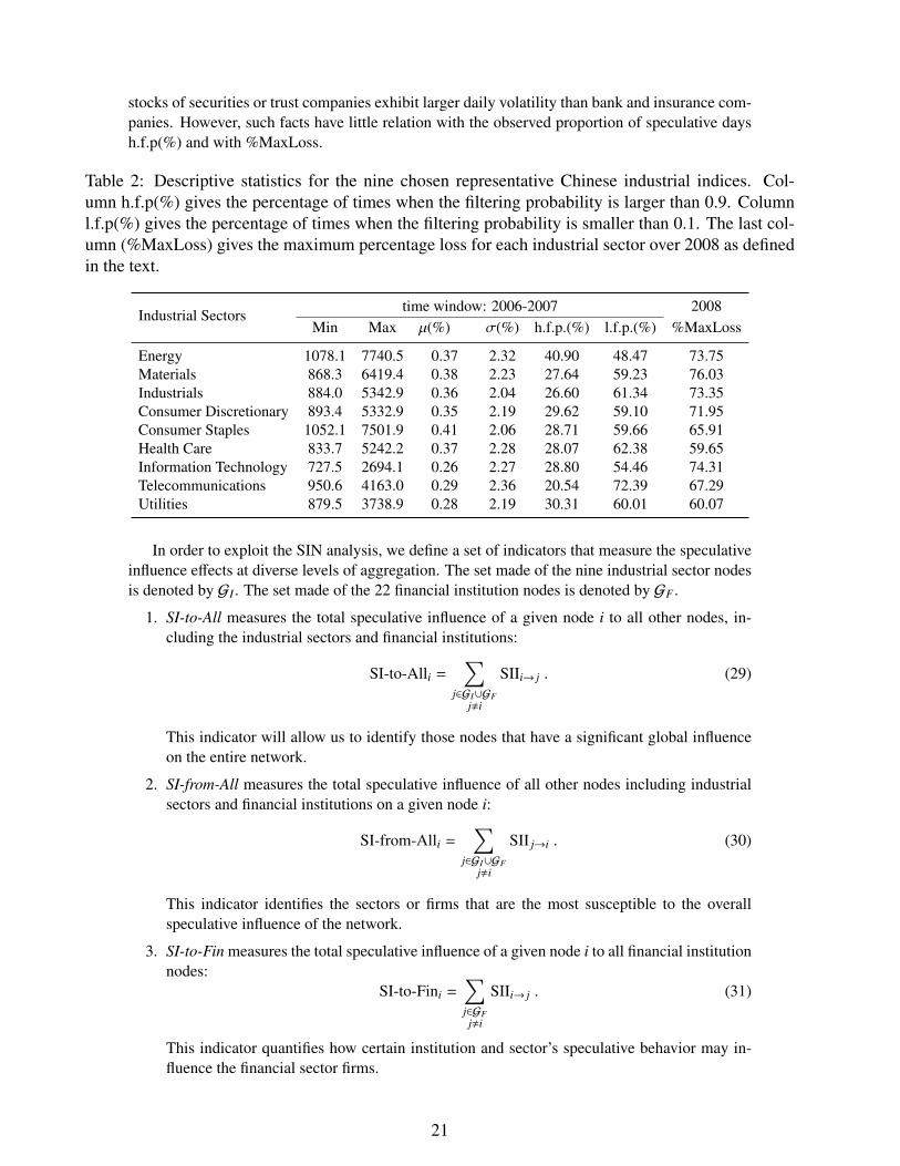
stocks of securities or trust companies exhibit larger daily volatility than bank and insurance com-panies. However, such facts have little relation with the observed proportion of speculative daysh.f.p(%) and with %MaxLoss.

Table 2: Descriptive statistics for the nine chosen representative Chinese industrial indices. Col-umn h.f.p(%) gives the percentage of times when the filtering probability is larger than 0.9. Columnl.f.p(%) gives the percentage of times when the filtering probability is smaller than 0.1. The last col-umn (%MaxLoss) gives the maximum percentage loss for each industrial sector over 2008 as definedin the text.

Industrial Sectorstime window: 2006-2007 2008

Min Max µ(%) σ(%) h.f.p.(%) l.f.p.(%) %MaxLoss

Energy 1078.1 7740.5 0.37 2.32 40.90 48.47 73.75Materials 868.3 6419.4 0.38 2.23 27.64 59.23 76.03Industrials 884.0 5342.9 0.36 2.04 26.60 61.34 73.35Consumer Discretionary 893.4 5332.9 0.35 2.19 29.62 59.10 71.95Consumer Staples 1052.1 7501.9 0.41 2.06 28.71 59.66 65.91Health Care 833.7 5242.2 0.37 2.28 28.07 62.38 59.65Information Technology 727.5 2694.1 0.26 2.27 28.80 54.46 74.31Telecommunications 950.6 4163.0 0.29 2.36 20.54 72.39 67.29Utilities 879.5 3738.9 0.28 2.19 30.31 60.01 60.07

In order to exploit the SIN analysis, we define a set of indicators that measure the speculativeinfluence effects at diverse levels of aggregation. The set made of the nine industrial sector nodesis denoted by GI . The set made of the 22 financial institution nodes is denoted by GF .

1. SI-to-All measures the total speculative influence of a given node i to all other nodes, in-cluding the industrial sectors and financial institutions:

SI-to-Alli =∑

j∈GI∪GFj,i

SIIi→ j . (29)

This indicator will allow us to identify those nodes that have a significant global influenceon the entire network.

2. SI-from-All measures the total speculative influence of all other nodes including industrialsectors and financial institutions on a given node i:

SI-from-Alli =∑

j∈GI∪GFj,i

SII j→i . (30)

This indicator identifies the sectors or firms that are the most susceptible to the overallspeculative influence of the network.

3. SI-to-Fin measures the total speculative influence of a given node i to all financial institutionnodes:

SI-to-Fini =∑j∈GFj,i

SIIi→ j . (31)

This indicator quantifies how certain institution and sector’s speculative behavior may in-fluence the financial sector firms.

21

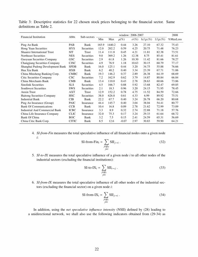
Table 3: Descriptive statistics for 22 chosen stock prices belonging to the financial sector. Samedefinitions as Table 2.

Financial Institution Abbr. Sub-sectorswindow: 2006-2007 2008

Min Max µ(%) σ(%) h.f.p.(%) l.f.p.(%) %MaxLoss

Ping An Bank PAB Bank 165.9 1440.2 0.44 3.26 27.10 67.32 75.43Hong Yuan Securities HYS Securities 12.0 202.2 0.59 4.25 20.75 71.48 76.23Shaanxi International Trust SIT Trust 11.4 111.8 0.45 4.21 11.81 82.38 73.51Northeast Securities NES Securities 9.0 369.2 1.26 12.38 8.75 85.41 81.61Guoyuan Securities Company GSC Securities 2.9 61.8 1.26 10.30 11.42 81.66 78.27Changjiang Securities Company CJSC Securities 4.9 76.9 1.18 10.63 30.15 60.79 77.17Shanghai Pudong Development Bank SPDB Bank 16.0 125.1 0.44 3.20 34.75 55.88 76.66Hua Xia Bank HXB Bank 6.2 40.2 0.40 3.34 23.39 67.71 71.06China Minsheng Banking Corp. CMBC Bank 19.3 146.2 0.37 2.89 26.38 64.19 68.69Citic Securities Company CSC Securities 7.2 162.9 0.62 3.79 14.87 80.84 66.84China Merchants Bank CMB Bank 13.4 110.0 0.43 2.78 28.63 60.66 73.86Sinolink Securities SLS Securities 4.5 166.7 0.88 5.92 13.68 82.47 69.85Southwest Securities SWS Securities 2.1 18.3 0.96 3.20 24.15 71.95 78.45Anxin Trust AXT Trust 12.9 152.2 0.78 4.75 11.52 84.59 72.66Haitong Securities Company HSC Securities 38.0 626.8 0.61 4.33 6.99 89.92 75.51Industrial Bank CIB Bank 22.2 67.7 0.40 3.24 26.78 66.20 80.68Ping An Insurance (Group) PAIC Insurance 44.4 145.7 0.40 3.04 38.04 54.41 80.77Bank Of Communications CCB Bank 10.4 16.8 0.09 2.78 21.62 72.99 73.09Industrial And Commercial Bank ICBC Insurance 3.3 8.9 0.32 2.74 22.88 71.18 57.76China Life Insurance Company CLIC Insurance 32.0 75.3 0.17 3.24 29.33 61.64 68.72Bank Of China BOC Bank 3.2 7.5 0.15 2.41 24.59 65.31 56.69China Citic Bank Corp. CITIC Bank 8.5 12.6 -0.07 2.97 30.83 59.90 64.21

4. SI-from-Fin measures the total speculative influence of all financial nodes onto a given nodei:

SI-from-Fini =∑j∈GFj,i

SII j→i . (32)

5. SI-to-IX measures the total speculative influence of a given node i to all other nodes of theindustrial sectors (excluding the financial institutions):

SI-to-IXi =∑j∈GIj,i

SIIi→ j . (33)

6. SI-from-IX measures the total speculative influence of all other nodes of the industrial sec-tors (excluding the financial sector) on a given node i:

SI-from-IXi =∑j∈GIj,i

SII j→i . (34)

In addition, using the net speculative influence intensity (NSII) defined by (28) leading toa unidirectional network, we shall also use the following indicators obtained from (29-34) as

22

follows:

NSII-on-Alli =∑

j∈GI∪GFj,i

NSIIi→ j = SI-to-Alli − SI-from-Alli (35)

NSII-on-Fini =∑j∈GFj,i

NSIIi→ j = SI-to-Fini − SI-from-Fini (36)

NSII-on-IXi =∑j∈GIj,i

NSIIi→ j = SI-to-IXi − SI-from-IXi . (37)

These indicators quantify the net speculative influence flux of a node to all the other nodes(NSII-on-Alli), to all financial nodes (NSII-on-Fini) and to all non-financial nodes (NSII-on-IXi).

We want to detect what combination of indicators for individual institution/sector performsbest as the leading factor during a bubble phase to explain the %MaxLoss of a given node asso-ciated with a large financial sell-offs during a bubble collapse. The corresponding leading factorsare good candidates to provide early-warning signals encoded in the SIN and to become systemicrisk metrics.

4.2 Early-warning signal extraction from the speculative influencenetwork (SIN)To evaluate the predictive power of SIN indicators defined above, we first perform multivariateregressions of %MaxLoss on different combinations of the 6 indicators (29-34). For the purposeof completeness and to avoid unnecessary multicollinearity, 17 regression models in total areselected. On the basis that industrial sectors and financial institutions play different roles, wesimplify the treatment by performing tests on group GF and group GI separately. The resultsare shown in tables 4 and 5. All indicators are constructed with data from 1st January 2006 to31st December 2007 and they are ranked before implementing the regressions. Without loss ofinformation and to avoid inflating the tables, we do not report the intercepts of the regressions.

For Chinese financial institutions, we find that SI-to-Fin and SI-from-Fin are both significantdeterminants to explain their maximum drawdown in 2008, while their impacts are of oppositesigns. The positive sign obtained for the ranked value of SI-to-Fin means that the more powerful isthe speculative herding influence of a node towards a financial institution, the larger is the loss ofthat node during the bubble burst. These results suggest the institutions with higher SI-to-Fin rankare more likely to act as the leading speculative engines of the overall speculative mania withinthe financial sector, with more inflow of speculative money during bubble. The negative signobtained for the ranked value of SI-from-Fin implies that the larger is the speculative influence offinancial institutions towards a given node, the stronger is the resilience of that node during thefinancial sell-offs. The institutions with higher SI-from-Fin rank are more likely to be lagging inthe speculative frenzy and may be less exposed to the bubble collapse.

Table 4 demonstrates that SI-to-IX has also a high explanatory power for the loss sizes ofindustrial institutions (excluding financial firms). However, different from SI-to-Fin, the larger thespeculative influence of a node on other industrial sector firms, the smaller is the loss during thecrash. In contrast, SI-from-IX has an insignificant effect, suggesting that there is little transmissionof speculation from the industry sectors to other firms. Additionally, table 4 also shows that SI-to-IX has a high explanatory power for the loss sizes of financial institutions. Again, differentfrom SI-to-Fin, the larger the speculative influence of a node on all nodes of the industrial sectors,the smaller is the loss during the crash for this financial institution. We also observe that the risktransfer between financial institutions and industrial sectors is not symmetric. Table 5 shows that

23

there is little influence of the variable SI-to-Fin onto the industrial sector concerning its loss size.Meanwhile, given the insignificance of the variable SI-from-IX to explain the losses of financialinstitutions shown in table 4, we conjecture that, during the bubble, the Chinese financial sectoras a whole only provided speculative money to other industrial sectors but did not absorb it backduring the crisis.

As shown in table 5, SI-to-IX and SI-from-IX both become significant determinants of thelosses of the industrial sector in 2008. This is very similar to the results obtained for financialinstitutions listed in table 4. This also suggests that the nodes that have the leading speculativeinfluence on their peers bear the largest loss risks, while the followers are less punished by the mar-ket correction. However, we failed to find SI-from-Fin to be a significant indicator for %MaxLossof industrial sectors. At first glance, this appears to be in contradiction with our previous conjec-ture that speculative money is more likely to go to industrial sectors, and taken out of financialinstitutions that have more influence onto industrial sectors as a whole. Noting that the financialsector as a whole is nothing but a peer node within the network of all industrial sectors, it is pos-sible that the total flow of speculative money emanating from the financial sector is not sufficientto increase the risk exposure of the industrial sectors for this Chinese bubble. The %MaxLoss ofindustrial sectors should be in large part explained by the overall circulation of speculative moneyamong all the nodes within the network rather than by the flow to and from a single node, such asthe financial sector. In other words, this shows the limit of a simple causal analysis of influences,suggesting the importance of a complex nonlinear set of mutual interactions that cannot be simplylinearly disentangled. In hindsight, this interpretation is also partially supported by the lack ofevidence of the presence of systemic risks spreading from the financial sector to other Chineseeconomic sectors through illiquidity, insolvency, or losses during the bubble collapse.

We also performed correlation tests between %MaxLoss and possible combinations of ourchosen indicators. To keep in line with the previously revealed relationships, the test first focuseson NSII and then associates NSII with a possible global influence effect for specific sub-networks,without making an exhaustive enumeration of all possible combinations. Similar to the aboveregression analysis, the tests are implemented separately on group GF and group GI . All combi-nations are ranked before testing. Table 6 presents the results based on three popular correlationstatistics. We find that NSII-on-IX outperforms other combinations to predict the rank of losssizes of industrial sectors. By taking account of other overall influence effects, the predictivepower decreases in agreement with our previous discussion of the regression analysis that the fi-nancial sector had very little influence in transferring risks to other industrial sectors during thisbubble. Nevertheless, NSII-on-Fin has only a modest correlation with the %MaxLoss for finan-cial institutions. However, when considering SI-from-IX, its predictive power increases nearlytwofold to become a significant signal. In agreement with our previous inference that financialinstitutions do not show significant tendencies to draw “hot money” from the real economy sectorbut act more as speculative followers, the present correlation estimations confirm that financialinstitutions are less important in China with respect to the systemic risks building up during thebubble, which is driven more by the real economy than the reverse.

To fully appreciate the impact of the relationships of speculation influence among variousindustrial sectors as well as financial institutions, Fig. 5 provides a visualization of the unidirec-tional SIN calculated by using data in the same time window as before (1st Jan. 2006 to 31 Dec.2007). This network is comprised of two sub-networks, the industrial sectors with 9 nodes andthe financial sub-network with 22 nodes. Recall that this financial network can be regarded as aspecial node in the former network but has been disaggregated as explained above.

First, the size of a node encodes the net transfer entropy (TE) from that node to all othernodes. To make the network representation comparable with the regression and correlation anal-yses presented above, we use a slightly different rule for the sizes of the nodes corresponding tothe industrial sectors and to the financial firms. For the industrial sector nodes, their sizes are

24

Tabl

e4:

Test

ofth

eex

plan

ator

ypo

wer

ofco

mbi

natio

nsof

indi

cato

rsde

scri

bed

inth

ete

xtfr

om1s

tJan

.20

06to

31st

Dec

.20

07to

pred

icti

tsM

ax%

Los

sov

er20

08of

the

seto

f22

finan

cial

inst

itutio

nno

desG

F,w

itha

mul

tiple

regr

essi

onan

alys

is.

The

rear

esi

xca

ndid

ate

expl

anat

ory

vari

able

sto

bech

osen

:SI

-fro

m-A

ll,SI

-to-

Fin,

SI-f

rom

-Fin

,SI-

to-I

X,S

I-fr

om-I

X.I

npr

actic

e,th

ese

expl

anat

ory

vari

able

sar

etr

ansf

orm

edin

toth

eir

cros

s-se

ctio

nally

rank

edva

lue

befo

reth

ere

gres

sion

s.

Mod

el1

Mod

el2

Mod

el3

Mod

el4

Mod

el5

Mod

el6

Mod

el7

Mod

el8

Mod

el9

Mod

el10

Mod

el11

Mod

el12

Mod

el13

Mod

el14

Mod

el15

Mod

el16

Mod

el17

SI-t

o-A

ll−

0.25

(0.2

3)SI

-fro

m-A

ll−

0.29

(0.2

2)SI

-to-

Fin

−0.

180.

030.

17−

0.11

1.06∗

0.02

0.25

1.17∗

(0.2

3)(0.2

2)(0.5

5)(0.2

2)(0.5

2)(0.2

3)(0.5

3)(0.5

8)SI

-fro

m-F

in−

0.23

−0.

38−

0.13

−0.

17−

1.05∗∗

−0.

39−

0.13

−1.

15∗∗

(0.2

3)(0.5

5)(0.2

1)(0.2

2)(0.4

9)(0.5

3)(0.2

1)(0.5

4)SI

-to-

IX−

0.53∗∗

−0.

54∗∗

−0.

50∗∗

−0.

48∗

−0.

74∗∗∗

−0.

49−

0.46

−0.

86∗∗

(0.2

0)(0.2

2)(0.2

1)(0.2

7)(0.2

3)(0.3

0)(0.2

8)(0.3

2)SI

-fro

m-I

X−

0.39

−0.

37−

0.07

−0.

36−

0.07

−0.

37−

0.07

0.14

(0.2

2)(0.2

2)(0.2

7)(0.2

2)(0.2

8)(0.2

3)(0.2

8)(0.2

8)

R2

0.06

0.08

0.03

0.26

0.05

0.14

0.26

0.05

0.15

0.27

0.26

0.17

0.41

0.26

0.18

0.27

0.42

Adj

.R2

0.01

0.03

-0.0

20.

22-0

.00

0.10

0.18

-0.0

50.

060.

200.

180.

080.

310.

140.

040.

150.

28F

stat

istic

1.24

1.64

0.58

6.90

0.99

3.24

3.29

0.52

1.68

3.56

3.33

1.88

4.11

2.11

1.27

2.27

3.02

∗∗∗p<

0.01

,∗∗p<

0.05

,∗p<

0.1

Tabl

e5:

Test

ofth

eex

plan

ator

ypo

wer

ofco

mbi

natio

nsof

indi

cato

rsde

scri

bed

inth

ete

xtfr

om1s

tJan

.20

06to

31st

Dec

.20

07to

pred

icti

tsM

ax%

Los

sov

er20

08of

the

set

ofni

nein

dust

rial

sect

orno

desG

I,w

itha

mul

tiple

regr

essi

onan

alys

is.

The

rear

esi

xca

ndid

ate

expl

anat

ory

vari

able

sto

bech

osen

:SI

-fro

m-A

ll,SI

-to-

IX,S

I-fr

om-I

X,S

I-to

-Fin

,SI-

from

-Fin

.In

prac

tice,

thes

eex

plan

ator

yva

riab

les

are

tran

sfor

med

into

thei

rcr

oss-

sect

iona

llyra

nked

valu

ebe

fore

the

regr

essi

ons.

Mod

el1

Mod

el2

Mod

el3

Mod

el4

Mod

el5

Mod

el6

Mod

el7

Mod

el8

Mod

el9

Mod

el10

Mod

el11

Mod

el12

Mod

el13

Mod

el14

Mod

el15

Mod

el16

Mod

el17

SI-t

o-A

ll0.

64(0.8

2)SI

-fro

m-A

ll0.

57(0.8

3)SI

-to-

IX1.

091.

111.

052.

48∗∗

1.20

2.48∗∗

2.43∗

2.55∗

(0.7

5)(0.7

8)(0.8

1)(0.9

1)(0.8

9)(0.9

4)(0.9

8)(1.0

6)SI

-fro

m-I

X−

0.07

−0.

05−

1.89∗

−0.

12−

1.86

−0.

08−

1.88

−1.

85(0.8

6)(0.9

0)(0.9

1)(0.9

1)(0.9

4)(1.0

2)(0.9

8)(1.0

4)SI

-to-

Fin

0.49

0.53

0.33

0.49

0.96

0.48

0.30

0.84

(0.8

4)(0.7

8)(1.6

3)(0.9

0)(1.6

0)(0.6

4)(1.8

4)(1.3

4)SI

-fro

m-F

in0.

460.

190.

310.

48−

0.51

0.22

0.29

−0.

43(0.8

4)(1.6

3)(0.8

1)(0.9

1)(1.6

2)(1.8

5)(0.6

7)(1.3

5)

R2

0.08

0.06

0.05

0.23

0.04

0.00

0.29

0.05

0.05

0.25

0.56

0.04

0.30

0.60

0.05

0.57

0.61

Adj

.R2

-0.0

5-0

.07

-0.0

90.

12-0

.09

-0.1

40.

05-0

.27

-0.2

70.

000.

41-0

.27

-0.1

20.

36-0

.52

0.31

0.22

Fst

atis

tic0.

620.

480.

342.

130.

310.

011.

210.

150.

151.

013.

750.

140.

722.

500.

092.

221.

57∗∗∗p<

0.01

,∗∗p<

0.05

,∗p<

0.1

25

Table 6: Correlations between %MaxLoss and different combinations of indicators given in the firstcolumn, as described in the text.

IndicatorsCorrelation Statistics

Pearson Spearman Kendall

For Industrial Sectors

NSII-on-All -0.06 -0.07 -0.06NSII-on-IX 0.41 0.42 0.28NSII-on-Fin -0.25 -0.28 -0.22NSII-on-IX−(SI-from-Fin) -0.14 -0.10 -0.06NSII-on-Fin−(SI-from-IX) -0.37 -0.32 -0.22NSII-on-IX+(SI-to-Fin) 0.22 0.27 0.17NSII-on-Fin+(SI-to-IX) 0.12 0.10 0.06

For Financial Institutions

NSII-on-All 0.29 0.20 0.13NSII-on-Fin 0.28 0.22 0.15NSII-on-IX 0.00 -0.06 -0.06NSII-on-Fin−(SI-from-IX) 0.47 0.39 0.30NSII-on-IX−(SI-from-Fin ) 0.21 0.06 0.06NSII-on-Fin+(SI-to-IX) 0.03 -0.02 -0.01NSII-on-IX+(SI-to-Fin) -0.22 -0.15 -0.14

determined by the rank value of their NSII-on-IX. For the financial institution nodes, their sizesare proportional to the ranked value of their NSII-on-Fin minus SI-from-IX.

In Fig. 5, all nodes are connected by their speculative influence relationship according to theNSII indicator defined by expression (28), i.e., an arrow from node X to Y indicates that X hasa net positive influence to foster speculative trading on Y . The thickness of each arrow encodesthe magnitude of the total of 465 NSIIs between 32 nodes. In details, the NSIIs are rescaled into[0, 1] by a dilation transformation. Then, the thicknesses of the edges in the SIN are proportionalto the rescaled NSIIs. To avoid overloading the figure, only the links with NSIIs that are above athreshold are represented with an arrow, as they represent the most important speculative influencerelationships. In practice, the threshold was chosen to be NSII ≥ 0.3, which yields 58 instancesthat account for approximately 10% of all links.

Finally, the color of a node encodes the rank of its %MaxLoss as shown on the scale in thefigure inset. The two different kinds of nodes (industry and finance) are considered separatelywhen calibrating the mapping function for node size and color.

Based on the colors and sizes of the nodes, the main information that emerges from Fig.5 is that the sectors or firms that lost the most are those influencing others most. The secondmessage of Fig. 5 is conveyed by the directions and thicknesses of the arrows. One can observethat some of the large nodes (e. g. Materials, Energy, CCB) receive many arrows pointing tothem. Given that their sizes encode the fact that they are the largest net influencers, the arrowspointing to them reveals a second order effect that they also receive large influences (above thethreshold NSII ≥ 0.3) from a few other sectors or firms. But these large influences only contributea maximum of 10% of the total influence relationships. Thus, it is more the overall influence overmost of the other sectors and firms that dominate the amplitude of the losses, rather than the (large)influence of a few. Rather than identifying a few systemically important sectors, the SIN analysis

26

emphasises the role of aggregated speculative influences in determining global interconnectednessand systemic risks. This interpretation is consistent with the results of the above regression andcorrelation analyses, which have concluded that larger Net Transfer Entropies lead to larger losses.

The case of CITIC is special, as it seems to act as a hub for important two-way speculativeinfluences between financial and industrial sub-networks. With smaller NSII-on-Fin minus SI-from-IX effect, this financial institution is, as expected, mildly punished during market correction.At first glance, The Information Technology sector seems to be an exception with little net entropytransfer to and from other industrial sectors but nevertheless a relative large loss. This can howeverbe rationalized by the important influence relationship from the financial sector (in particularCITIC) that might also signal an invisible “hot money” transfer between the sector before the fullforce of speculative herding revealed itself.

5 ConclusionWe have introduced the Speculative Influence Network (SIN) to represent the causal relationshipsbetween sectors (and/or firms) during financial bubbles. The construction of SIN required twosteps. First, we have shown how to estimate in real time the probability of speculative trading ineach stock in the basket of interest, using a bubble identifying technique based on the Sornette-Andersen (2002) stochastic bubble model. We have augmented the Sornette-Andersen (2002)model by using a Hidden Markov Model (HMM), which was specially designed to calibrateregime-switching between normal and bubble regimes. Conditional on two stocks or two sectorsbeing qualified in a bubble regime, we have introduced the Transfer Entropy, which quantifies thecasual relationship between them. The transfer entropy provided a natural way to construct anadjacency matrix and thus to introduce the SIN. We have applied this methodology to the Chinesestock market during the period 2005-2008, during which a normal phase was followed by a spec-tacular bubble ending in a massive correction. Introducing the Net Speculative Influence Intensity(NSII) variable as the difference between the transfer entropies from i to j and from j to i, wehave demonstrated its skill to predict the maximum loss (%MaxLoss) endured during the crashby the sectors and stocks. The statistically significant regressions and the graphical network rep-resentation has allowed us to llustrate the matrix of influences among sectors during the Chinesebubble. One the most striking result is the importance of the industrial sectors in influencing thefinancial firms and not vice-versa, showing a very different interaction structure than in westernmarkets. We have also shown that the bubble state variable calibrated on the Chinese market datacorresponds well to the regimes when the market exhibits a strong price acceleration followed byclear change of price regimes.

27

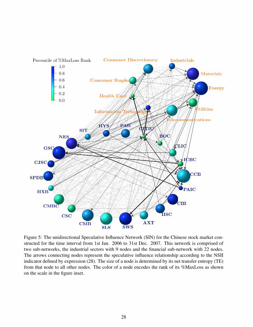
Figure 5: The unidirectional Speculative Influence Network (SIN) for the Chinese stock market con-structed for the time interval from 1st Jan. 2006 to 31st Dec. 2007. This network is comprised oftwo sub-networks, the industrial sectors with 9 nodes and the financial sub-network with 22 nodes.The arrows connecting nodes represent the speculative influence relationship according to the NSIIindicator defined by expression (28). The size of a node is determined by its net transfer entropy (TE)from that node to all other nodes. The color of a node encodes the rank of its %MaxLoss as shownon the scale in the figure inset.

28

A “Bra-ket” notations for probability formulasThis appendix introduces a convenient mathematical representation of probability distributionfunctions and of conditional density functions using notations involving bra-vector and ket-vector,according to the following definition:

1a. A single ”bra-vector” 〈 A | means the unconditional probability for A.

1b. A single ”ket-vector” |B 〉 indicates the conditions where event B is assumed to happen.

2a. Scalar-multiplication for “bra-vector” satisfies the commutative law: k · 〈 A | = 〈 A | · k, k ∈ R

2b. Scalar-multiplication for “ket-vector” satisfies the commutative law: k · |B 〉 = |B 〉 · k, k ∈ R

3 The multiplication between a single “bra” and a single “ket” vector makes a complete pair-wise bra-ket 〈 A | B 〉, which represents the conditional distribution f (A | B). The bra-ketcan be regarded as a number.

4a. The notation |A 〉〈 A | to concatenate a single “ket” vector and a single “bra” vector definesthe operator to transform a “ket” (“bra”) into another “ket” (“bra”), which leads to

• 〈 B |(|A 〉〈 A |

)= 〈 B | A 〉〈 A | = 〈 BA |

•(|A 〉〈 A |

)|B 〉 = |AB 〉 · 〈 A | B 〉

4b. Given A =⋃i

Ai, then∑

i |Ai 〉〈 Ai | = |1 〉〈 1 | := I where I = |1 〉〈 1 | denotes the identical

operator such that 〈 B |(|1 〉〈 1 |) = (〈 B | 1 〉)〈 1 | = f (B|1)〈 1 |, where 1 denotes the wholeuniverse, and thus 〈 1 | = p(1) = 1 and f (B|1) := f (B) = 〈 B | so that 〈 B |(|1 〉〈 1 |) = 〈 B |.

Further, according to the previous defined notations, the classic conditional probability andBayesian formula can be rewritten as

• (Conditional probability formula): 〈 A | B 〉 =〈 AB |〈 B |

or 〈 AB | = 〈 A | B 〉〈 B |

• (The Bayesian formula): 〈 A | B 〉 = 〈 A |〈 B | A 〉〈 B |

With the listed formal rules and the basic formula, we can easily give the derivations for thefollowing famous formula in probability theory.

1. (The Law of Total probability): 〈 A | = 〈 A | I = 〈 A | ·∑

i |Bi 〉〈 Bi | =∑

i〈 A | Bi 〉〈 Bi |

2. (Decomposed Conditional Joint Density):

〈 A, B | C 〉 = 〈 AB | · |C 〉 = (〈 A | B 〉〈 B |) · |C 〉

= 〈 A |(|B 〉〈 B |

)|C 〉 = 〈 A | · |BC 〉〈 B | C 〉

= 〈 A | B,C 〉〈 B | C 〉

3. (Multivariate Bayesian Formula):

〈 A | B,C 〉 =〈 A | BC 〉〈 B | C 〉〈 B | C 〉

=〈 A | ( |B 〉〈 B | ) |C 〉

〈 B | C 〉

=〈 AB | · |C 〉〈 B | C 〉

=〈 BA | · |C 〉〈 B | C 〉

=〈 B | ( |A 〉〈 A | ) |C 〉

〈 B | C 〉

= 〈 A | C 〉〈 B | A,C 〉〈 B | C 〉

29

B Proof of eq.(10)Proof. Since p−n

t | p−nt−1 ∼ N(p−n

t−1 − nµ1, n2σ21), one can get

〈 p−nt | p

−nt−1 〉 =

1√

2πσ1exp

−12·

(p−n

t − p−nt−1 − µ1

σ1

)2 . (38)

With the density transformation formula fx|y(x|y) = fx|y(φ(x)|y)|φ′(x)|, or equivalently〈 x | y 〉 = 〈 φ(x) | y 〉 · |φ′(x)|, eq.(38) further leads to

〈 pt | pt−1 〉 =1

√2π · nσ1

exp

−12·

(p−n

t − p−nt−1 + nµ1

nσ1

)2 · np−(n+1)t (39)

From the definition yt = ln pt, and using the density transformation formula again, we obtain

〈 yt | yt−1 〉 = 〈 eyt | yt−1 〉eyt = 〈 pt | yt 〉pt (40)

=1

√2π · nσ1

exp

−12·

(e−nyt − e−nyt−1 + nµ1

nσ1

)2 · ne−nyt (41)

Consequently, we have

ln〈 yt | 1, 1, yt−1 〉 = −12

ln 2π − ln nσ1 −12·

(e−nyt − e−nyt−1 + nµ1

nσ1

)2

+ ln n − nyt (42)

�

C Derivations for the equations in EM algorithm

C.1 proof of the eq. (14) from eq.(13)Proof.

lnLθθθ |θθθ(k−1) =∑1···T

ln〈 yT(, s

T( |θθθ 〈 y

T(, s

T( |θθθ(k−1) =

∑1···T

ln( 〈 yT( | s

T( 〉θθθ〈 sT

( |θθθ ) 〈 yT(, s

T( |θθθ(k−1)

=∑1···T

ln〈 yT( | s

T( 〉θθθ 〈 y

T(, s

T( |θθθ(k−1) +

∑1···T

ln〈 sT( |θθθ 〈 y

T(, s

T( |θθθ(k−1) (43)

For the first item in the r.h.s. of (43), we can further obtain

∑1···T

ln〈 yT( | s

T( 〉θθθ 〈 y

T(, s

T( |θθθ(k−1) =

∑1···T

T∑t=1

ln〈 yt | st, st−1, yt−1( 〉θθθ

〈 yT(, s

T( |θθθ(k−1)

=

T∑t=1

∑t,t−1

∑/t,/t−1

ln〈 yt | st, st−1, yt−1( 〉θθθ 〈 y

T(, s

T( |θθθ(k−1)

=

T∑t=1

∑t,t−1

ln〈 yt | st, st−1, yt−1( 〉θθθ

∑/t,/t−1

〈 yT(, s

T( |θθθ(k−1)

=

T∑t=1

∑t,t−1

ln〈 yt | st, st−1, yt−1( 〉θθθ 〈 y

T(, st, st−1 |θθθ(k−1)

= 〈 yT

( |θθθ(k−1)

T∑t=1

∑t,t−1

ln〈 yt | st, st−1, yt−1( 〉θθθ 〈 st−1, st | yT

( 〉θθθ(k−1)

30

where the notation∑/t,/t−1

represents the summation for all states sτ, τ = 1, · · · ,T , except for st−1

and st. The second term in the r.h.s. of (43) leads to

∑1···T

ln〈 sT( |θθθ 〈 y

T(, s

T( |θθθ(k−1) =

∑1···T

T∑t=1

ln〈 st | st−1 〉θθθ

〈 yT(, s

T( |θθθ(k−1)

=

T∑t=1

∑t,t−1

∑/t,/t−1

ln〈 st | st−1 〉θθθ 〈 yT(, s

T( |θθθ(k−1)

=

T∑t=1

∑t,t−1

ln〈 st | st−1 〉θθθ

∑/t,/t−1

〈 yT(, s

T( |θθθ(k−1)

= 〈 yT

( |θθθ(k−1)

T∑t=1

∑t,t−1

ln〈 st | st−1 〉θθθ 〈 st−1, st | yT( 〉θθθ(k−1)

Thus, we finally obtain (14)

lnLθθθθθθθθθ(k) |θθθ(k−1) = 〈 yT( |θθθ(k−1) ·

T∑

t=1

∑st=1,0

st−1=1,0

(ln〈 yt | st, st−1, yt−1 〉θθθ(k) + ln〈 st | st−1 〉θθθ(k)

)〈 st−1, st | yT

( 〉θθθ(k−1)

�

C.2 Derivation of the formulas to determine the first four parame-ters of the HMMSince 〈 sT

( |θθθ does not depend on θθθ = (µ0, σ0, µ1, σ1, n), one can ignore the second term in eq. (43)when calibrating the parameters of the HMM.

In order to compute µ(k)0 , the first-order condition of the first term in eq. (43) reads

T∑t=1

∑

st=1,0st−1=1,0

∂

∂µ0ln〈 yt | st, st−1, yt−1 〉θθθ 〈 st, st−1 | yT

( 〉θθθ(k−1)

= 0 (44)

which leads to

T∑t=1

(yt − yt−1 − µ0

σ0〈 st = 0, st−1 = 0 | yT

( 〉θθθ(k−1)

)= 0

=⇒ µ0 =

∑Tt=1(yt − yt−1)〈 st = 0, st−1 = 0 | yT

( 〉θθθ(k−1)∑Tt=1〈 st = 0, st−1 = 0 | yT

( 〉θθθ(k−1)

=⇒ µ(k)0 =

∑Tt=1 ω

(k−1)(0,0);t(yt − yt−1)∑Tt=1 ω

(k−1)(0,0);t

In order to compute σ(k)0 , the first-order condition of the first term in eq. (43) reads

T∑t=1

∑

st=1,0st−1=1,0

∂

∂σ0ln〈 yt | st, st−1, yt−1 〉θθθ 〈 st, st−1 | yT

( 〉θθθ(k−1)

= 0 (45)

31

which leads to

T∑t=1

− 1σ0

+(yt − yt−1 − µ0)2

σ30

〈 st = 0, st−1 = 0 | yT( 〉θθθ(k−1) = 0

=⇒ σ(k)0 =

√√√√∑Tt=1 ω

(k−1)(0,0);t(yt − yt−1 − µ

(k)0 )2∑T

t=1 ω(k−1)(0,0);t

In order to compute µ(k)1 , the first-order condition of the first term in eq. (43) reads

T∑t=1

∑

st=1,0st−1=1,0

∂

∂µ1ln〈 yt | st, st−1, yt−1 〉θθθ 〈 st, st−1 | yT

( 〉θθθ(k−1)

= 0 (46)

which leads to

T∑t=1

− p−nt − p−n

t−1 + nµ1

nσ21

〈 st = 1, st−1 = 1 | yT( 〉θθθ(k−1) = 0

=⇒

T∑t=1

(−p−n

t + p−nt−1 − nµ1

)ω(k−1)

(1,1);t = 0

=⇒ µ(k)1 =

∑Tt=1 ω

(k−1)(1,1);t(p−n

t−1 − p−nt )

n∑T

t=1 ω(k−1)(1,1);t

In order to compute σ(k)1 , the first-order condition of the first term in eq. (43) reads

T∑t=1

∑

st=1,0st−1=1,0

∂

∂σ1ln〈 yt | st, st−1, yt−1 〉θθθ 〈 st, st−1 | yT

( 〉θθθ(k−1)

= 0 (47)

which leads to

T∑t=1

1σ1−

(p−nt − p−n

t−1 + nµ1)2

n2σ31

〈 st = 1, st−1 = 1 | yT( 〉θθθ(k−1) = 0

=⇒

T∑t=1

[(p−n

t − p−nt−1 + nµ1)2 − n2σ2

1

]ω(k−1)

(1,1);t = 0

=⇒ σ(k)1 =

√√√√∑Tt=1 ω

(k−1)(1,1);t(p−n

t − p−nt−1 + nµ(k)

1 )2

n2 ∑Tt=1 ω

(k−1)(1,1);t

C.3 Derivation for eq.(15) to solve for nTo compute n(k), one should solve the first-order condition of the first term in eq. (43) with respectto n, that is

T∑t=1

∑

st=1,0st−1=1,0

∂

∂nln〈 yt | st, st−1, yt−1 〉θθθ 〈 st, st−1 | yT

( 〉θθθ(k−1)

= 0 (48)

32

which gives,

T∑t=1

(−

(p−nt − p−n

t−1 + nµ1)(−p−nt ln pt + p−n

t−1 ln pt−1 + µ1)

n2σ21

+(p−n

t − p−nt−1 + nµ1)2

n3σ21

−1n

+1n− ln pt

)ω(k−1)

(1,1):t = 0 (49)

Note thatT∑

t=1

(p−nt − p−n

t−1 + nµ1)2

n3σ21

−1n

ω(k−1)(1,1):t = 0. Thus, the above equation can be reduced

to

T∑t=1

− (p−nt − p−n

t−1 + nµ1)(−p−nt ln pt + p−n

t−1 ln pt−1 + µ1)

n2σ21

+1n− ln pt

ω(k−1)(1,1):t = 0 (50)

C.4 Derivation of the formulas to compute the optimal posterior tran-sition probability from st−1 to st

Since 〈 st | st−1 〉θθθ(k) is only related to the second term in eq.(43), we can ignore the first term whenperforming the optimization:

∑1···T

ln〈 sT( |θθθ 〈 y

T(, s

T( |θθθ(k−1) =

T∑t=1

∑t,t−1

ln〈 st | st−1 〉θθθ 〈 st, st−1 | yT( 〉θθθ(k−1)

=

T∑t=1

∑j,i

ln q(k)i j 〈 j, i | yT

( 〉θθθ(k−1)

Without loss of generality, the first-order condition against qi1 leads to

0 =

T∑t=1

∂

∂q(k)i1

ln q(k)i j 〈 i, j | yT

( 〉θθθ(k−1)

=

T∑t=1

1

q(k)i1

〈 1, i | yT( 〉θθθ(k−1) −

1

1 − q(k)i1

〈 0, i | yT( 〉θθθ(k−1)

Then we have

q(k)i1 =

∑Tt=1〈 1, i | y

T( 〉θθθ(k−1)∑T

t=1(〈 1, i | yT( 〉θθθ(k−1) + 〈 0, i | yT

( 〉θθθ(k−1))=

∑Tt=1〈 1, i | y

T( 〉θθθ(k−1)∑T

t=1〈 i | yT( 〉θθθ(k−1)

It is the optimal posterior transition probability after the kth iteration, q(k)i j , when j = 1.

33

C.5 Reasoning to replace 〈 st | st+1, yt(, y

(t+1 〉 by 〈 st | st+1, yt

( 〉 ineq.(20)

〈 st | st+1, yt(, y

(t+1 〉 =

〈 st |

(|st+1, yt

(, y(t+1 〉

)〈 y(t+1 | st+1, yt

( 〉

〈 y(t+1 | st+1, yt( 〉

(51)

=

〈 st |

(|st+1, yt

(, y(t+1 〉 〈 y

(t+1 | st+1, yt

( 〉

)〈 y(t+1 | st+1, yt

( 〉(52)

=

〈 st |

(|y(t+1 〉〈 y

(t+1 |

)|st+1, yt

( 〉

〈 y(t+1 | st+1, yt( 〉

(53)

=

(〈 st | y(t+1 〉〈 y

(t+1 |

)|st+1, yt

( 〉

〈 y(t+1 | st+1, yt( 〉

=

〈 y(t+1 |

(|st 〉〈 st |

)|st+1, yt

( 〉

〈 y(t+1 | st+1, yt( 〉

(54)

=〈 y(t+1 | st, st+1, yt

( 〉〈 st | st+1, yt( 〉

〈 y(t+1 | st+1, yt( 〉

(55)

By assuming that the joint distribution of (yt+1, yt+2, · · · , yT ) is irrelevent to st, we can elimi-nate the denominator and easily recover (55) for 〈 st | st+1, yt

( 〉

34

ReferencesAndersen, J., Sornette, D., 2004. Fearless versus fearful speculative financial bubbles. Physica A:

Statistical Mechanics and its Applications 337 (3-4), 565–585.

Ardila-Alvarez, D., Forro, Z., Sornette, D., 2015. The acceleration effect and gamma factor inasset pricing. Swiss Finance Institute Research Paper No. 15-30. Available at SSRN: http://ssrn.com/abstract=2645882.

Avery, C., Zemsky, P., 1998. Multidimensional uncertainty and herd behavior in financial markets.American Economic Review 88 (4), 724–748.

Banerjee, A. V., 1992. A simple model of herd behavior. The Quarterly Journal of Economics107 (3), 797–817.

Barberis, N., Shleifer, A., Vishny, R., 1998. A model of investor sentiment. Journal of FinancialEconomics 49 (3), 307–343.

Barnett, L., Barrett, A. B., Seth, A. K., 2009. Granger causality and transfer entropy are equivalentfor Gaussian variables. Physical Review Letters 103 (23), 238701.

Barrett, A. B., Barnett, L., 2013. Granger causality is designed to measure effect, not mechanism.Frontiers in Neuroinformatics 7 (6), 1–2.

Bikhchandani, S., Hirshleifer, D., Welch, I., 1992. A theory of fads, fashion, custom, and culturalchange as informational cascades. Journal of Political Economy 100 (5), 992–1026.

Brunnermeier, M. K., Oehmke, M., 2013. Bubbles, financial crises, and systemic risk. Handbookof the Economics of Finance. Amsterdam: Elsevier 2 (B), 1221–1288.

Cajueiro, D., Tabak, B., Werneck, F., 2009. Can we predict crashes? The case of the Brazilianstock market. Physica A: Statistical Mechanics and its Applications 388 (8), 1603–1609.

Chiang, T. C., Li, J., Tan, L., 2010. Empirical investigation of herding behavior in chinese stockmarkets: Evidence from quantile regression analysis. Global Finance Journal 21 (1), 111–124.

Chincarini, L. B., 2012. The Crisis of Crowding: Quant Copycats, Ugly Models, and the NewCrash Normal. John Wiley & Sons.

Choi, N., Sias, R. W., 2009. Institutional industry herding. Journal of Financial Economics 94 (3),469–491.

Dass, N., Massa, M., Patgiri, R., 2008. Mutual funds and bubbles: The surprising role of contrac-tual incentives. Review of Financial Studies 21 (1), 51–99.

Dempster, A. P., Laird, N. M., Rubin, D. B., 1977. Maximum likelihood from incomplete data viathe EM algorithm. Journal of the Royal Statistical Society. Series B (Methodological) 39 (1),1–38.

Devenow, A., Welch, I., 1996. Rational herding in financial economics. European Economic Re-view 40 (3), 603–615.

Dimitriadi, G., 2004. What are ”financial bubbles” : Approaches and definitions. Electronic Jour-nal “INVESTIGATED in RUSSIA”.

35

Filimonov, V., Sornette, D., 2013. A stable and robust calibration scheme of the log-periodicpower law model. Physica A-Statistical Mechanics and Its Applications 392 (17), 3698–3707.

Giordano, M., Mannella, R., 2006. A brief analysis of may 2004 crash in the indian market.Fluctuation and Noise Letters 6 (3), 243–249.

Gurkaynak, R. S., 2008. Econometric tests of asset price bubbles: taking stock. Journal of Eco-nomic Surveys 22 (1), 166–186.

Hamilton, J. D., 1989. A new approach to the economic analysis of nonstationary time series andthe business cycle. Econometrica: Journal of the Econometric Society 57 (2), 357–384.

He, Z., Su, D., 2009. Price manipulation and industry momentum: Evidence from the chinesestock market. Available at SSRN: http://ssrn.com/abstract=1393505.

Hlavackova-Schindler, K., 2011. Equivalence of granger causality and transfer entropy: a gener-alization. Applied Mathematical Sciences 5 (73), 3637–3648.

Hong, H., Kubik, J. D., Stein, J. C., 2005. Thy neighbor’s portfolio: Word-of-mouth effects in theholdings and trades of money managers. Journal of Finance 60 (6), 2801–2824.

Husler, A., Sornette, D., Hommes, C. H., 2013. Super-exponential bubbles in lab experiments:evidence for anchoring over-optimistic expectations on price. Journal Economic Behavior andOrganization 92, 304–316.

Ide, K., Sornette, D., 2002. Oscillatory finite-time singularities in finance, population and rupture.Physica A 307 (1-2), 63–106.

Jeanblanc, M., Yor, M., Chesney, M., 2009. Mathematical Methods for Financial Markets.Springer Finance, Springer Finance Textbooks.

Jiang, Z.-Q., Zhou, W.-X., Sornette, D., Woodard, R., Bastiaensen, K., Cauwels, P., 2010. Bub-ble diagnosis and prediction of the 2005-2007 and 2008-2009 chinese stock market bubbles.Journal of Economic Behavior & Organization 74 (3), 149–162.

Johansen, A., Ledoit, O., Sornette, D., 2000. Crashes as critical points. International Journal ofTheoretical and Applied Finance 3, 219–255.

Johansen, A., Sornette, D., 2000. The nasdaq crash of april 2000: Yet another example of log-perodicity in a speculative bubble ending in a crash. European Physical Journal B 17, 319–328.

Johansen, A., Sornette, D., 2001. Bubbles and anti-bubbles in latin-american, asian and westernstock markets: an empirical study. International Journal of Theoretical and Applied Finance4 (6), 853–920.

Johansen, A., Sornette, D., Ledoit, O., 1999. Predicting financial crashes using discrete scaleinvariance. Journal of Risk 1 (4), 5–32.

Kaizoji, T., Leiss, M., Saichev, A., Sornette, D., 2015. Super-exponential endogenous bubbles inan equilibrium model of rational and noise traders. Journal of Economic Behavior and Organi-zation 112, 289–310.

Khwaja, A. I., Mian, A., 2005. Unchecked intermediaries: Price manipulation in an emergingstock market. Journal of Financial Economics 78 (1), 203–241.

36

Kim, C.-J., Nelson, C. R., 1999. State-space models with regime switching. Cambridge, Mass.

Lakonishok, J., Shleifer, A., Vishny, R. W., 1994. Contrarian investment, extrapolation, and risk.The journal of Finance 49 (5), 1541–1578.

Leiss, M., Nax, H., Sornette, D., 2015. Super-exponential growth expectations and the globalfinancial crisis. Journal of Economic Dynamics and Control 55, 1–13.

Li, W., Rhee, G., Wang, S. S., 2009. Differences in herding: individual vs. institutional investorsin china. Institutional Investors in China (SSRN: February 13, 2009).

Lin, L., Ren, R.-E., Sornette, D., 2014. The volatility-confined LPPL model: A consistent modelof ‘explosive’financial bubbles with mean-reverting residuals. International Review of Finan-cial Analysis 33, 210–225.

Lin, L., Sornette, D., 2013. Diagnostics of rational expectation financial bubbles with stochasticmean-reverting termination times. The European Journal of Finance 19 (5), 344–365.

Long, J. B. D., Shleifer, A., Summers, L. H., Waldmann, R. J., 1990. Noise trader risk in financialmarkets. Journal of Political Economy 98 (4), 703–738.

Matsushita, R., da Silva, S., Figueiredo, A., Gleria, I., 2006. Log-periodic crashes revisited. Phys-ica A: Statistical Mechanics and its Applications 364, 331–335.

Nofsinger, J. R., Sias, R. W., 1999. Herding and feedback trading by institutional and individualinvestors. The Journal of Finance 54 (6), 2263–2295.

Piotroski, J. D., Wong, T., 2011. Institutions and information environment of chinese listed firms.In: Capitalizing China. University of Chicago Press, pp. 201–242.

Redner, S., 2001. A Guide to First-Passage Processes. Cambridge University Press.

Roehner, B. M., Sornette, D., 2000. “Thermometers” of speculative frenzy. The European Physi-cal Journal B-Condensed Matter 16 (4), 729–739.

Shiller, R. J., 2000. Irrational exuberance. Princeton University Press, NJ.

Sias, R. W., 2004. Institutional herding. Review of Financial Studies 17 (1), 165–206.

Sornette, D., 1998. Discrete-scale invariance and complex dimensions. Physics Reports 297, 239–270.

Sornette, D., Andersen, J. V., 2002. A nonlinear super-exponential rational model of speculativefinancial bubbles. International Journal of Modern Physics C 13 (2), 171–188.

Sornette, D., Cauwels, P., 2014. 1980-2008: The illusion of the perpetual money machine andwhat it bodes for the future. Risks 2, 103–131.

Sornette, D., Cauwels, P., 2015. Financial bubbles: mechanisms and diagnostics. Review of Be-havioral Economics 2 (3), http://ssrn.com/abstract=2423790.

Sornette, D., Demos, G., Zhang, Q., Cauwels, P., Filimonov, V., Zhang, Q., 2015. Real-timeprediction and post-mortem analysis of the Shanghai 2015 stock market bubble and crash.Journal of Investment Strategies 4 (4), 77–95.

37

Sornette, D., Johansen, A., 1998. A hierarchical model of financial crashes. Physica A: StatisticalMechanics and Its Applications-Statistical Mechanics and Its Applications 261, 581–598.

Sornette, D., Woodard, R., 2010. Financial bubbles, real estate bubbles, derivative bubbles, andthe financial and economic crisis. Proceedings of APFA7 (Applications of Physics in FinancialAnalysis), “New Approaches to the Analysis of Large-Scale Business and Economic Data,”Misako Takayasu, Tsutomu Watanabe and Hideki Takayasu, eds., Springer, http://arxiv.org/abs/0905.0220.

Sornette, D., Woodard, R., Zhou, W. X., 2009. The 2006–2008 oil bubble: Evidence of specula-tion, and prediction. Physica A: Statistical Mechanics and its Applications 388, 1571–1576.

Sornette, D., Zhou, W.-X., 2006. Predictability of large future changes in major financial indices.International Journal of Forecasting 22, 153–168.

Tan, L., Chiang, T. C., Mason, J. R., Nelling, E., 2008. Herding behavior in chinese stock markets:An examination of a and b shares. Pacific-Basin Finance Journal 16 (1), 61–77.

Xu, N.-X., Yu, S.-R., Yin, Z. H., 2013. Institutional investor herding and stock price crash risk.Management World (Chinese) (7), 31–43.

Zhou, C.-S., Yang, Y. H., Wang, Y.-P., 2005. Trading-based market manipulation in china’s stockmarket. Economic Research Journal (In Chinese) 10.

Zhou, W. X., Sornette, D., 2006a. Fundamental factors versus herding in the 2000-2005 us stockmarket and prediction. Physica A: Statistical Mechanics and Its ApplicationsStatistical Me-chanics and Its Applications 360 (2), 459–482.

Zhou, W. X., Sornette, D., 2006b. Is there a real-estate bubble in the us? Physica A-StatisticalMechanics and Its Applications 361 (1), 297–308.

Zhou, W.-X., Sornette, D., 2008. Analysis of the real estate market in las vegas: Bubble, seasonalpatterns, and prediction of the csw indexes. Physica A: Statistical Mechanics and its Applica-tions 387, 243–260.

Zhou, W.-X., Sornette, D., 2009. A case study of speculative financial bubbles in the South Africanstock market 2003-2006. Physica A: Statistical Mechanics and its Applications 388, 869–880.

38