spectral simplicity of apparent complexity, part i: the ... › sfi-edu › ... · part ii, to the...
TRANSCRIPT
Spectral Simplicity of ApparentComplexity, Part I: TheNondiagonalizableMetadynamics of PredictionPaul M. RiechersJames P. Crutchfield
SFI WORKING PAPER: 2017-05-018
SFIWorkingPaperscontainaccountsofscienti5icworkoftheauthor(s)anddonotnecessarilyrepresenttheviewsoftheSantaFeInstitute.Weacceptpapersintendedforpublicationinpeer-reviewedjournalsorproceedingsvolumes,butnotpapersthathavealreadyappearedinprint.Exceptforpapersbyourexternalfaculty,papersmustbebasedonworkdoneatSFI,inspiredbyaninvitedvisittoorcollaborationatSFI,orfundedbyanSFIgrant.
©NOTICE:Thisworkingpaperisincludedbypermissionofthecontributingauthor(s)asameanstoensuretimelydistributionofthescholarlyandtechnicalworkonanon-commercialbasis.Copyrightandallrightsthereinaremaintainedbytheauthor(s).Itisunderstoodthatallpersonscopyingthisinformationwilladheretothetermsandconstraintsinvokedbyeachauthor'scopyright.Theseworksmayberepostedonlywiththeexplicitpermissionofthecopyrightholder.
www.santafe.edu
SANTA FE INSTITUTE
Santa Fe Institute Working Paper 17-05-XXXarxiv.org:1705.XXXX [nlin.CD]
Spectral Simplicity of Apparent Complexity, Part I:The Nondiagonalizable Metadynamics of Prediction
Paul M. Riechers∗ and James P. Crutchfield†
Complexity Sciences CenterDepartment of Physics
University of California at DavisOne Shields Avenue, Davis, CA 95616
(Dated: May 22, 2017)
Virtually all questions that one can ask about the behavioral and structural complexity of astochastic process reduce to a linear algebraic framing of a time evolution governed by an appropri-ate hidden-Markov process generator. Each type of question—correlation, predictability, predictivecost, observer synchronization, and the like—induces a distinct generator class. Answers are thenfunctions of the class-appropriate transition dynamic. Unfortunately, these dynamics are generi-cally nonnormal, nondiagonalizable, singular, and so on. Tractably analyzing these dynamics relieson adapting the recently introduced meromorphic functional calculus, which specifies the spectraldecomposition of functions of nondiagonalizable linear operators, even when the function poles andzeros coincide with the operator’s spectrum. Along the way, we establish special properties of theprojection operators that demonstrate how they capture the organization of subprocesses within acomplex system. Circumventing the spurious infinities of alternative calculi, this leads in the sequel,Part II, to the first closed-form expressions for complexity measures, couched either in terms ofthe Drazin inverse (negative-one power of a singular operator) or the eigenvalues and projectionoperators of the appropriate transition dynamic.
PACS numbers: 02.50.-r 89.70.+c 05.45.Tp 02.50.Ey 02.50.GaKeywords: hidden Markov model, entropy rate, excess entropy, predictable information, statistical complex-ity, projection operator, complex analysis, resolvent, Drazin inverse
CONTENTS
I. Introduction 1
II. Structured Processes and their Complexities 3A. Directly observable organization 4B. Intrinsic predictability 4C. Prediction overhead 5D. Generative complexities 6
III. Hidden Markov Models 6A. Unifilar HMMs 7B. Minimal unifilar HMMs 7C. Finitary stochastic process hierarchy 8D. Continuous-time HMMs 8
IV. Mixed-State Presentations 8
V. Identifying the Hidden Linear Dynamic 10A. Simple complexity from any presentation 10B. Predictability from a presentation MSP 11C. Continuous time? 12D. Synchronization from generator MSP 12E. Optimal prediction from ε-machine MSP 13F. Beyond the MSP 13G. The end? 14
∗ [email protected]† [email protected]
VI. Spectral Theory beyond the Spectral Theorem 15A. Spectral primer 15B. Eigenprojectors: Left, right, generalized 15C. Companion operators and resolvent
decomposition 16D. Functions of nondiagonalizable operators 17E. Evaluating residues 17F. Decomposing AL 17G. Drazin inverse 18
VII. Projection Operators for Stochastic Dynamics 18A. Row sums 19B. Expected stationary distribution 19
VIII. Spectra by inspection 19A. Eigenvalues 20B. Eigenprojectors from graph structure 21
IX. Conclusion 21
Acknowledgments 21
References 22
I. INTRODUCTION
Complex systems—that is, many-body systems with
strong interactions—are usually observed through low-
resolution feature detectors. The consequence is that
their hidden structure is, at best, only revealed over time.
2
Since individual observations cannot capture the full res-
olution of each degree of freedom, let alone a sufficiently
full set of them, measurement time series often appear
stochastic and non-Markovian, exhibiting long-range cor-
relations. Empirical challenges aside, restricting to the
purely theoretical domain, even finite systems can ap-
pear quite complicated. Despite admitting finite descrip-
tions, stochastic processes with sofic support, to take one
example, exhibit infinite-range dependencies among the
chain of random variables they generate [1]. While such
infinite-correlation processes are legion in complex physi-
cal and biological systems, even approximately analyzing
them is generally appreciated as difficult, if not impossi-
ble. Generically, even finite systems lead to uncountably
infinite sets of predictive features [2]. These facts seem to
put physical sciences’ most basic goal—prediction—out
of reach.
We aim to show that this direct, but sobering conclu-
sion is too bleak. Rather, there is a collection of con-
structive methods that address hidden structure and the
challenges associated with predicting complex systems.
This follows up on our recent introduction of a func-
tional calculus that uncovered new relationships among
supposedly different complexity measures [3] and that
demonstrated the need for a generalized spectral theory
to answer such questions [4]. Those efforts yielded ele-
gant, closed-form solutions for complexity measures that,
when compared, offered insight into the overall theory
of complexity measures. Here, providing the necessary
background for and greatly expanding those results, we
show that different questions regarding correlation, pre-
dictability, and prediction each require their own ana-
lytical structures, expressed as various kinds of hidden
transition dynamic. The resulting transition dynamic
among hidden variables summarizes symmetry breaking,
synchronization, and information processing, for exam-
ple. Each of these metadynamics, though, is built up
from the original given system.
The shift in perspective that allows the new level of
tractability begins by recognizing that—beyond their
ability to generate many sophisticated processes of
interest—hidden Markov models can be treated as ex-
act mathematical objects when analyzing the processes
they generate. Crucially, and especially when addressing
nonlinear processes, most questions that we ask imply a
linear transition dynamic over some hidden state space.
Speaking simply, something happens, then it evolves lin-
early in time, then we snapshot a selected characteristic.
This broad type of sequential questioning cascades, in
the sense that the influence of the initial preparation cas-
cades through state space as time evolves, affecting the
final measurement. Alternatively, other, complementary
kinds of questioning involve accumulating such cascades.
Linear Algebra Underlying ComplexityQuestion type Discrete time Continuous time
Cascading 〈·|TL|·〉 〈·|etG|·〉Accumulating 〈·|
(∑L T
L)|·〉 〈·|
(∫etG dt
)|·〉
TABLE I. Having identified the hidden linear dynamic, ei-ther a discrete-time operator T or continuous-time operatorG, quantitative questions tend to be either cascading or ac-cumulating type. What changes between distinct questionsare the dot products with the initial setup 〈·| and the finalobservations |·〉.
The linear algebra underlying either kind is highlighted
in Table I in terms of an appropriate discrete-time transi-
tion operator T or a continuous-time generator G of time
evolution.
In this way, deploying linear algebra to analyze com-
plex systems turns on identifying an appropriate hidden
state space. And, in turn, the latter depends on the
genre of the question. Here, we focus on closed-form
expressions for a process’ complexity measures. This de-
termines what the internal system setup 〈·| and the final
detection |·〉 should be. We show that complexity ques-
tions fall into three subgenres and, for each of these, we
identify the appropriate linear dynamic and closed-form
expressions for several of the key questions in each genre.
See Table II. The burden of the following is to explain the
table in detail. We return to a much-elaborated version
at the end.
Associating observables x ∈ A with transitions be-
tween hidden states s ∈ S, gives a hidden Markov
model (HMM) with observation-labeled transition ma-
trices{T (x) : T
(x)i,j = Pr(x, sj |si)
}x∈A. They sum to
the row-stochastic state-to-state transition matrix T =∑x∈A T
(x). (The continuous-time versions are similarly
defined, which we do later on.) Adding measurement
symbols x ∈ A this way—to transitions—can be consid-
ered a model of measurement itself [5]. The efficacy of
our choice will become clear.
It is important to note that HMMs, in continuous
and discrete time, arise broadly in the sciences, from
quantum mechanics [6, 7], statistical mechanics [8], and
stochastic thermodynamics [9–11] to communication the-
ory [12, 13], information processing [14–16], computer de-
sign [17], population and evolutionary dynamics [18, 19],
and economics. Thus, HMMs appear in the most funda-
mental physics and in the most applied engineering and
social sciences. The breadth suggests that the thorough-
going HMM analysis developed here is worth the required
effort.
Since complex processes have highly structured, direc-
tional transition dynamics—T or G—we encounter the
3
full richness of matrix algebra in analyzing HMMs. We
explain how analyzing complex systems induces a nondi-
agonalizable metadynamics, even if the original dynamic
is diagonalizable in its underlying state-space. Normal
and diagonalizable restrictions, so familiar in mathemat-
ical physics, simply fail us here.
The diversity of nondiagonalizable dynamics presents
a technical challenge, though. A new calculus for func-
tions of nondiagonalizable operators—e.g., TL or etG—
becomes a necessity if one’s goal is an exact analysis
of complex processes. Moreover, complexity measures
naively and easily lead one to consider illegal operations.
Taking the inverse of a singular operator is a particu-
larly central, useful, and fraught example. Fortunately,
such illegal operations can be skirted since the complex-
ity measures only extract the excess transient behavior
of an infinitely complicated orbit space.
To explain how this arises—how certain modes of be-
havior, such as excess transients, are selected as relevant,
while others are ignored—Ref. [4] recently developed a
meromorphic functional calculus for analyzing complex
processes generated by HMMs. The following shows that
this leads to a general spectral theory of weighted di-
rected graphs and that, more specifically, the techniques
can be applied to the challenges of prediction. The results
developed here greatly extend and (finally) explain those
announced in Ref. [3]. The latter introduced the basic
methods and results by narrowly focusing on closed-form
expressions for several measures of intrinsic computation,
applying them to prototype complex systems.
The meromorphic functional calculus, summarized in
detail later, concerns functions of nondiagonalizable op-
erators when poles (or zeros) of the function of inter-
est coincide with poles of the operator’s resolvent—poles
that appear precisely at the eigenvalues of the transition
dynamics. Pole–pole and pole–zero interactions trans-
form the complex-analysis residues within the functional
calculus. One notable result is that the negative-one
power of a singular operator exists in the meromorphic
functional calculus. We derive its form, note that it is the
Drazin inverse, and show how widely useful and common
it is.
For example, the following gives the first closed-form
expressions for many complexity measures in wide use—
many of which turn out to be expressed most concisely
in terms of a Drazin inverse. Furthermore, spectral de-
composition gives insight into subprocesses of a complex
system in terms of the projection operators of the appro-
priate transition dynamic.
To get started, sections §II through §III briefly review
relevant background in stochastic processes, the HMMs
that generate them, and complexity measures. Several
classes of HMMs are discussed in §III. Mixed-state pre-
Questions and Their Linear DynamicsGenre Measures Hidden dynamic
ObservationCorrelations γ(L)
HMM matrix TPower spectra P (w)
PredictabilityMyopic entropy hµ(L) HMM MSPExcess entropy E, E(w) matrix W
PredictionCausal Cµ, H+(L) ε-Machine MSP
synchrony S, S(w) matrix WGeneration
State Cµ(M), Generatorsynchrony H(L), S′ MSP matrix
TABLE II. Question genres (leftmost column) about processcomplexity listed with increasing sophistication. Each genreimplies a different linear transition dynamic (rightmost col-umn). Observational questions concern the superficial, givendynamic. Predictability questions are about the observation-induced dynamic over distributions; that is, over states usedto generate the superficial dynamic. Prediction questions ad-dress the dynamic over distributions over a process’ causally-equivalent histories. Generation questions concern the dy-namic over any nonunifilar presentation M.
sentations (MSPs)—HMM generators of a process that
also track distributions induced by observation—are re-
viewed in §IV. They are key to complexity measures
within an information-theoretic framing. Section §V then
shows how each complexity measure reduces to the linear
algebra of an appropriate HMM adapted to the question
genre.
To make progress at this point, we summarize the
meromorphic functional calculus in §VI. Several of its
mathematical implications are discussed in relation to
projection operators in §VII and a spectral weighted di-
rected graph theory is presented in §VIII.
With this all set out, the sequel Part II finally de-
rives the promised closed-form complexities of a process
and outlines common simplifications for special cases.
Leveraging the functional calculus, it introduces a novel
extension—the complexity measure frequency spectrum
and shows how to calculate it in closed form. It provides a
suite of examples to ground the theoretical developments
and works through in-depth a pedagogical example.
II. STRUCTURED PROCESSES AND THEIR
COMPLEXITIES
We first describe a system of interest in terms of
its observed behavior, following the approach of com-
putational mechanics, as reviewed in Ref. [20]. Again,
a process is the collection of behaviors that the sys-
tem produces and their probabilities of occurring.
A process’s behaviors are described via a bi-infinite
chain of random variables, denoted by capital letters

4
. . . Xt−2Xt−1XtXt+1Xt+2 . . .. A realization is indi-
cated by lowercase letters . . . xt−2 xt−1 xt xt+1 xt+2 . . ..
We assume values xt belong to a discrete alphabet A.
We work with blocks Xt:t′ , where the first index is inclu-
sive and the second exclusive: Xt:t′ = Xt . . . Xt′−1. Block
realizations xt:t′ we often refer to as words w. At each
time t, we can speak of the past X−∞:t = . . . Xt−2Xt−1
and the future Xt:∞ = XtXt+1 . . ..
A process’s probabilistic specification is a density over
these chains: P(X−∞:∞). Practically, we work with fi-
nite blocks and their probability distributions Pr(Xt:t′).
To simplify the development, we primarily analyze sta-
tionary, ergodic processes: those for which Pr(Xt:t+L) =
Pr(X0:L) for all t ∈ Z, L ∈ Z+, and all realizations. In
such cases, we only need to consider a process’s length-L
word distributions Pr(X0:L).
A. Directly observable organization
A common first step to understand how processes ex-
press themselves is to analyze correlations among observ-
ables. Pairwise correlation in a sequence of observables
is often summarized by the autocorrelation function:
γ(L) =⟨XtXt+L
⟩t,
where the bar above Xt denotes its complex conjugate,
and the angled brackets denote an average over all times
t ∈ Z. Alternatively, structure in a stochastic process
is often summarized by the power spectral density, also
referred to more simply as the power spectrum:
P (ω) = limN→∞
1
N
⟨∣∣∣∣N∑
L=1
XLe−iωL
∣∣∣∣2⟩
,
where ω ∈ R is the angular frequency [21]. Though a ba-
sic fact, it is not always sufficiently emphasized in appli-
cations that power spectra capture only pairwise correla-
tion. Indeed, it is straightforward to show that the power
spectrum P (ω) is the windowed Fourier transform of the
autocorrelation function γ(L). That is, power spectra
describe how pairwise correlations are distributed across
frequencies. Power spectra are common in signal process-
ing, both in technological settings and physical experi-
ments [22]. As a physical example, diffraction patterns
are the power spectra of a sequence of structure factors
[23].
To monitor transport properties in near-equilibrium
thermodynamic systems, the Green–Kubo coefficients
are another important example measure of observable or-
ganization, but are rather more application-specific [24,
25]. These coefficients reflect the idea that dissipation
depends on correlation structure. They usually appear
in the form of integrating the autocorrelation of deriva-
tives of observables. A change of observables, however,
turns this into an integration of a standard autocorre-
lation function. Green–Kubo transport coefficients then
involve the limit limω→0 P (ω) for the process of appro-
priate observables.
One theme in the following is that, though widely used,
correlation functions and power spectra give an impover-
ished view of a process’s structural complexity, since they
only consider ensemble averages over pairwise events.
Moreover, creating a list of higher-order correlations is
an impractical way to summarize complexity, as seen in
the connected correlation functions of statistical mechan-
ics [26].
B. Intrinsic predictability
Information measures, in contrast, can involve all or-
ders of correlation and thus help to go beyond pairwise
correlation in understanding, for example, how a process’
past behavior affects predicting it at later times. In-
formation theory, as developed for general complex pro-
cesses [1], provides a suite of quantities that capture pre-
diction properties using variants of Shannon’s entropy
H[·] and mutual information I[ · ; · ] [13] applied to se-
quences. Each measure answers a specific question about
a process’ predictability. For example:
• How much information is contained in the words
generated? The block entropy [1]:
H(L) = −∑
w∈ALPr(w) log2 Pr(w) .
• How random is a process? Its entropy rate [27]:
hµ = limL→∞
H(L)/L .
• How is the irreducible randomness hµ approached?
Via the myopic entropy rates [1]:
hµ(L) = H[X0|X1−L . . . X−1] .
• How much of the future can be predicted? Its excess
entropy [1]:
E = I[X−∞:0;X0:∞] .
• How much information must be extracted to know its
5
predictability and so see its intrinsic randomness
hµ? Its transient information [1]:
T =
∞∑
L=0
[E + hµL−H(L)] .
The spectral approach, our subject, naturally leads to
allied, but new information measures. To give a sense,
later we introduce the excess entropy spectrum E(ω).
It completely, yet concisely, summarizes the structure
of myopic entropy reduction, in a way similar to how
the power spectrum completely describes autocorrela-
tion. However, while the power spectrum summarizes
only pairwise linear correlation, the excess entropy spec-
trum captures all orders of nonlinear dependency be-
tween random variables, making it an incisive probe of
hidden structure.
Before leaving the measures related to predictabil-
ity, we must also point out that they have important
refinements—measures that lend a particularly useful,
even functional, interpretation. These include the bound,
ephemeral, elusive, and related informations [28, 29].
Though amenable to the spectral methods of the follow-
ing, we leave their discussion for another venue. Fortu-
nately, their spectral development is straightforward, but
would take us beyond the minimum necessary presenta-
tion to make good on the overall discussion of spectral
decomposition.
C. Prediction overhead
Process predictability measures, as just enumerated,
certainly say much about a process’ intrinsic information
processing. They leave open, though, the question of
the structural complexity associated with implementing
prediction. This challenge entails a complementary set of
measures that directly address the inherent complexity of
actually predicting what is predictable. For that matter,
how cryptic is a process?
Computational mechanics describes optimal prediction
via a process’ hidden, effective or causal states and tran-
sitions, as summarized by the process’s ε-machine [20].
A causal state σ ∈ S+ is an equivalence class of histo-
ries X−∞:0 that all yield the same probability distribu-
tion over observable futures X0:∞. Therefore, knowing
a process’s current causal state—that S+0 = σ, say—is
sufficient for optimal prediction.
Computational mechanics provides an additional suite
of quantities that capture the overhead of prediction,
again using variants of Shannon’s entropy and mutual
information applied to the ε-machine. Each also answers
a specific question about an observer’s burden of predic-
tion. For example:
• How much historical information must be stored for
optimal prediction? The statistical complexity [30]:
Cµ = H[S+0 ] .
• How unpredictable is a causal state upon observing a
process for duration L? The myopic causal-state
uncertainty [1]:
H+(L) = H[S+0 |X−L . . . X−1] .
• How much information must an observer extract to
synchronize to—that is, to know with certainty—
the causal state? The optimal predictor’s synchro-
nization information [1]:
S =
∞∑
L=0
H+(L) .
Paralleling the purely informational suite of the previ-
ous section, we later introduce the optimal synchroniza-
tion spectrum S(ω). It completely and concisely sum-
marizes the frequency distribution of state-uncertainty
reduction, similar to how the power spectrum P (ω) com-
pletely describes autocorrelation and the excess entropy
spectrum E(ω) the myopic entropy reduction. Helpfully,
the above optimal prediction measures can be found from
the optimal synchronization spectrum.
The structural complexities monitor an observer’s bur-
den in optimally predicting a process. And so, they have
practical relevance when an intelligent artificial or biolog-
ical agent must take advantage of a structured stochastic
environment—e.g., a Maxwellian Demon taking advan-
tage of correlated environmental fluctuations [31], prey
avoiding easy prediction, or profiting from stock market
volatility, come to mind.
Prediction has many natural generalizations. For ex-
ample, since optimal prediction often requires infinite
resources, suboptimal prediction is of practical interest.
Fortunately, there are principled ways to investigate the
tradeoffs between predictive accuracy and computational
burden [2, 32–34]. As another example, optimal predic-
tion in the presence of noisy or irregular observations
can be investigated with a properly generalized frame-
work; see Ref. [35]. Blending the existing tools, resource-
limited prediction under such observational constraints
can also be investigated. In all of these settings, infor-
mation measures similar to those listed above are key
to understanding and quantifying the tradeoffs arising in
prediction.
Having highlighted the difference between prediction
and predictability, we can appreciate that some processes
6
hide more internal information—are more cryptic—than
others. It turns out, this can be quantified. The cryp-
ticity χ = Cµ − E is the difference between the a pro-
cess’s stored information Cµ and the mutual information
E shared between past and future observables [36]. Op-
erationally, crypticity contrasts predictable information
content E with an observer’s minimal stored-memory
overhead Cµ required to make predictions. To predict
what is predictable, therefore, an optimal predictor must
account for a process’s crypticity.
D. Generative complexities
How does a physical system produce its output pro-
cess? This depends on many details. Some systems em-
ploy vast internal mechanistic redundancy, while others
under constraints have optimized internal resources down
to a minimally necessary generative structure. Different
pressures give rise to different kinds of optimality. For ex-
ample, minimal state-entropy generators turn out to be
distinct from minimal state-set generators [37–39]. The
challenge then is to develop ways to monitor differences
in generative mechanism.
Any generative model [1, 40] M with state-set R has
a statistical complexity (state entropy): C(M) = H[R].
Consider the corresponding myopic state-uncertainty
given L sequential observations:
H(L) = H[R0|X−L:0] ,
And so:
H(0) = C(M) .
We also have the asymptotic uncertainty H ≡limL→∞H(L). Related, there is the excess synchroniza-
tion information:
S′ =
∞∑
L=0
[H(L)−H
].
Such quantities are relevant even when an observer never
fully synchronizes to a generative state; i.e., even when
H > 0. Finite-state ε-machines always synchronize [41,
42] and so their H vanishes.
Since many different mechanisms can generate a given
process, we need useful bounds on the statistical com-
plexity of possible process generators. For example, the
minimal generative complexity Cg = min{R} C(M) is the
minimal state-information a physical system must store
to generate its future [39]. The predictability and the
statistical complexities bound each other:
E ≤ Cg ≤ Cµ .
That is, the predictable future information E is less than
or equal to the information Cg necessary to produce the
future which, in turn, is less than or equal to the in-
formation Cµ necessary to predict the future [1, 37–39].
Such relationships have been explored even for quantum
generators of (classical) stochastic processes [43, and ref-
erences therein].
III. HIDDEN MARKOV MODELS
Up to this point, the development focused on introduc-
ing and interpreting various information and complexity
measures. It was not constructive in that there was no
specification of how to calculate these quantities for a
given process. To do so requires models or, in the ver-
nacular, a presentation of a process. Fortunately, a com-
mon mathematical representation describes a wide class
of process generators: the edge-labeled hidden Markov
models (HMMs), also known as a Mealy HMMs [40] [44].
Using these as our preferred presentations, we will first
classify them and then describe how to calculate the in-
formation measures of the processes they generate.
Definition 1. A finite-state, edge-labeled hidden
Markov model M ={R,A, {T (x)}x∈A, η0
}consists of:
• A finite set of hidden states R = {ρ1, . . . , ρM}. Rt is
the random variable for the hidden state at time t.
• A finite output alphabet A.
• A set of M × M symbol-labeled transition matrices{T (x)
}x∈A, where T
(x)i,j = Pr(x, ρj |ρi) is the proba-
bility of transitioning from state ρi to state ρj and
emitting symbol x. The corresponding overall state-
to-state transition matrix is the row-stochastic ma-
trix T =∑x∈A T
(x).
• An initial distribution over hidden states: η0 =(Pr(R0 = ρ1),Pr(R0 = ρ2), ...,Pr(R0 = ρM )
).
The dynamics of such finite-state models are governed
by transition matrices amenable to the linear algebra of
vector spaces. As a result, bra-ket notation is useful [45].
Bras 〈·| are row vectors and kets |·〉 are column vectors.
One benefit of the notation is immediately recognizing
mathematical object type. For example, on the one hand,
any expression that forms a closed bra-ket pair—either
〈·|·〉 or 〈·| · |·〉—is a scalar quantity and commutes as a
unit with anything. On the other hand, when useful, an
expression of the ket-bra form |·〉 〈·| can be interpreted as
a matrix.
7
T ’s row-stochasticity means that each of its rows sum
to unity. Introducing |1〉 as the column vector of all 1s,
this can be restated as:
T |1〉 = |1〉 .
This is readily recognized as an eigenequation: T |η〉 =
λ |η〉. That is, the all-ones vector |1〉 is always a right
eigenvector of T associated with the eigenvalue λ of unity.
When the internal Markov transition matrix T is ir-
reducible, the Perron-Frobenius theorem guarantees that
there is a unique asymptotic state distribution π deter-
mined by:
〈π|T = 〈π| ,
with the further condition that π is normalized in prob-
ability: 〈π|1〉 = 1. This again is recognized as an
eigenequation: the asymptotic distribution π over the
hidden states is T ’s left eigenvector associated with the
eigenvalue of unity.
To describe a stationary process, as done often in the
following, the initial hidden-state distribution η0 is set
to the asymptotic one: η0 = π. The resulting process
generated is then stationary. Choosing an alternative η0
is useful in many contexts, but yields a nonstationary
process. We avoid this for now for simplicity.
An HMM M describes a process’ behaviors as a for-
mal language L ⊆ ⋃∞`=1A` of allowed realizations. More-
over, M succinctly describes a process’s word distribu-
tion Pr(w) over all words w ∈ L. (Appropriately,M also
assigns zero probability to words outside of the process’
language: Pr(w) = 0 for all w ∈ Lc, L’s complement.)
Specifically, the stationary probability of observing a par-
ticular length-L word w = x0x1 . . . xL−1 is given by:
Pr(w) = 〈π|T (w) |1〉 , (1)
where T (w) ≡ T (x0)T (x1) · · ·T (xL−1).
More generally, given a nonstationary state distribu-
tion η, the subsequent probability of a word is:
Pr(Xt:t+L = w|Rt ∼ η) = 〈η|T (w) |1〉 , (2)
where Rt ∼ η means that the random variable Rt is dis-
tributed as η [13]. This conditional word probability is
used often since, for example, most observations induce
a nonstationary distribution over hidden states. Track-
ing such observation-induced distributions is the role of
a related model class—the mixed-state presentation, in-
troduced shortly. To get there, we must first introduce
several, prerequisite HMM classes. See Fig. 1. The gen-
eral HMM just discussed is shown in Fig. 1a.
A. Unifilar HMMs
An important class of HMMs consists of those that are
unifilar. Unifilarity guarantees that, given a start state
and a sequence of observations, there is a unique path
through the internal states [46]. This, in turn, allows one
to directly translate properties of the internal Markov
chain into properties of the observed behavior generated
from the sequence of edges traversed. Unifilar HMMs are
a process’ optimal predictors [47].
In contrast, general—that is, nonunifilar—HMMs have
an exponentially growing number of possible state paths
as a function of observed word length. Thus, nonunifilar
process presentations break most all quantitative connec-
tions between internal dynamics and observations, ren-
dering them markedly less useful process presentations.
While they can be used to generate realizations of a given
process, they cannot be used to predict a process. Unifi-
larity is required.
Definition 2. A finite-state, edge-labeled, unifilar HMM
(uHMM) [48] is a finite-state, edge-labeled HMM with the
following property:
• Unifilarity: For each state ρ ∈ R and each symbol
x ∈ A there is at most one outgoing edge from state
ρ that emits symbol x.
An example is shown in Fig. 1b.
B. Minimal unifilar HMMs
Minimal models are not only convenient to use, but
very often allow for determining essential informational
properties, such as a process’ memory Cµ. A process’
minimal state-entropy uHMM is the same as its minimal-
state uHMM. And, the latter turns out to be the pro-
cess’ ε-machine in computational mechanics [20]. Com-
putational mechanics shows how to calculate a process’
ε-machine from the process’ conditional word distribu-
tions. Specifically, ε-machine states, the process’ causal
states σ ∈ S, are equivalence classes of histories that
yield the same predictions for the future. Explicitly,
two histories ←−x and ←−x ′ map to the same causal state
ε(←−x ) = ε(←−x ′) = σ if and only if Pr(−→X |←−x ) = Pr(
−→X |←−x ′).
Thus, each causal state comes with a prediction of the
future Pr(−→X |σ)—its future morph. In short, a process’
ε-machine is its minimal size, optimal predictor.
Converting a given uHMM to its corresponding
ε-machine employs probabilistic variants of well-known
state-minimization algorithms in automata theory [49].
One can also verify that a given uHMM is minimal by
checking that all its states are probabilistically distinct
[41, 42].
8
Definition 3. A uHMM’s states are probabilistically
distinct if for each pair of distinct states ρk, ρj ∈R there
exists some finite word w = x0x1 . . . xL−1 such that:
Pr(−→X = w|R = ρk) 6= Pr(
−→X = w|R = ρj) .
If this is the case, then the process’ uHMM is its
ε-machine.
An example is shown in Fig. 1c.
C. Finitary stochastic process hierarchy
The finite-state presentations in these classes form a
hierarchy in terms of the processes they can finitely gen-
erate [37]: Processes(ε-machines) = Processes(uHMMs)
⊂ Processes(HMMs). That is, finite HMMs generate a
strictly larger class of stochastic processes than finite uH-
MMs. The class of processes generated by finite uHMMs,
though, is the same as generated by finite ε-machines.
D. Continuous-time HMMs
Though we concentrate on discrete-time processes,
many of the process classifications, properties, and cal-
culational methods carry over easily to continuous time.
In this setting transition rates are more appropriate than
transition probabilities. Continuous-time HMMs can of-
ten be obtained as a discrete-time limit ∆t → 0 of
an edge-labeled HMM whose edges operate for a time
∆t. The most natural continuous-time HMM presenta-
tion, though, has a continuous-time generator G of time
evolution over hidden states, with observables emitted
as deterministic functions of an internal Markov chain:
f : S → A.
Respecting the continuous-time analogue of probabil-
ity conservation, each row of G sums to zero. Over a fi-
nite time interval t, marginalizing over all possible obser-
vations, the row-stochastic state-to-state transition dy-
namic is:
Tt0→t0+t = etG .
The generated process, a function of the internal
continuous-time Markov chain, can also be specified by a
set of transition matrices. For this purpose we introduce
the continuous-time observation matrices:
Γx =∑
ρ∈Rδx,f(ρ) |δρ〉 〈δρ| ,
where δx,f(ρ) is a Kronecker delta, |δρ〉 the column vector
of all zeros except for a one at the position for state ρ,
and 〈δρ| its transpose(|δρ〉)>
. These “projectors” sum
to the identity:∑x∈A Γx = I.
An example is shown in Fig. 1d.
IV. MIXED-STATE PRESENTATIONS
A given process can be generated by nonunifilar, unifi-
lar, and ε-machine HMM presentations. Within either
the unifilar or nonunifilar HMM classes, there can be an
unbounded number of presentations that generate the
process. A process’ ε-machine is unique, however.
This flexibility suggests that we can create a HMM
process generator to answer more refined questions than
information generation (hµ) and memory (Cµ) calcu-
lated from the ε-machine. To this end, we introduce the
mixed-state presentation (MSP). An MSP tracks impor-
tant supplementary information in the hidden states and,
through well-crafted dynamics, over the hidden states.
In particular, an MSP generates a process while tracking
the observation-induced distribution over the states of an
alternative process generator. Here, we review only that
subset of mixed-state theory required by the following.
Consider a HMM presentation M =(R,A, {T (x)}x∈A, π
)of some process in statistical
equilibrium. A mixed state η can be any state distribu-
tion over R, but the uncountable set of points in the
most general state-distribution simplex is infinitely more
than needed to calculate many complexity measures.
How to monitor the way in which an observer comes to
know the HMM state as it sees successive symbols from
the process? This is the problem of observer-state syn-
chronization. To analyze this evolution of the observer’s
knowledge, we use the set Rπ of mixed states that are
induced by all allowed words w ∈ L from initial mixed
state η0 = π:
Rπ =⋃
w∈L
〈π|T (w)
〈π|T (w) |1〉 .
The cardinality of Rπ is finite when there are only a
finite number of distinct probability distributions over
M’s states that can be induced by observed sequences,
if starting from the stationary distribution π.
If w is the first (in lexicographic order) word that in-
duces a particular distribution over R, then we denote
this distribution as ηw. For example, if the two words 010
and 110110 both induce the same distribution η over Rand no word shorter than 010 induces that distribution,
then the mixed state is denoted η010. It corresponds to
9
0 0 1
�2a
2a
b
�a� b
a
c
2b
�2b� c
.
0:12
2:12
1 : p
0 : 1� p
1 : p
0:12
2:12
0 : 1� p
.
0:12
2:12
1 : p 0 : 1� p
1 : p
0:12
2:12
0 : 1� p
.
1 : p
0 : 1� p
1 : 1
.
0 : p
0 : 1� p
1 : q
0 : 1� q
.
0
0
-1
-1
-1
-1
-1
1
2
3
1
1� b
1
1
11
1
b
1 1
1� b
b
.
10
(a) Nonunifilar HMM
0 0 1
�2a
2a
b
�a� b
a
c
2b
�2b� c
.
0:12
2:12
1 : p
0 : 1� p
1 : p
0:12
2:12
0 : 1� p
.
0:12
2:12
1 : p 0 : 1� p
1 : p
0:12
2:12
0 : 1� p
.
1 : p
0 : 1� p
1 : 1
.
0 : p
0 : 1� p
1 : q
0 : 1� q
.
0
0
-1
-1
-1
-1
-1
1
2
3
1
1� b
1
1
11
1
b
1 1
1� b
b
.
10
(b) Unifilar HMM
0 0 1
�2a
2a
b
�a� b
a
c
2b
�2b� c
.
0:12
2:12
1 : p
0 : 1� p
1 : p
0:12
2:12
0 : 1� p
.
0:12
2:12
1 : p 0 : 1� p
1 : p
0:12
2:12
0 : 1� p
.
1 : p
0 : 1� p
1 : 1
.
0 : p
0 : 1� p
1 : q
0 : 1� q
.
0
0
-1
-1
-1
-1
-1
1
2
3
1
1� b
1
1
11
1
b
1 1
1� b
b
.
10
(c) ε-machine
0 0 1
�2a
2a
b
�a� b
a
c
2b
�2b� c
.
0:12
2:12
1 : p
0 : 1� p
1 : p
0:12
2:12
0 : 1� p
.
0:12
2:12
1 : p 0 : 1� p
1 : p
0:12
2:12
0 : 1� p
.
1 : p
0 : 1� p
1 : 1
.
0 : p
0 : 1� p
1 : q
0 : 1� q
.
0
0
-1
-1
-1
-1
-1
1
2
3
1
1� b
1
1
11
1
b
1 1
1� b
b
.
10
(d) Continuous-time function of aMarkov chain
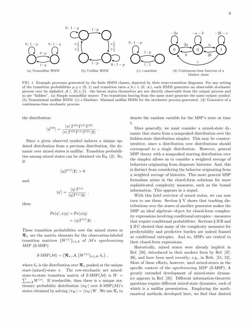
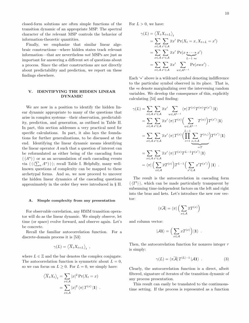
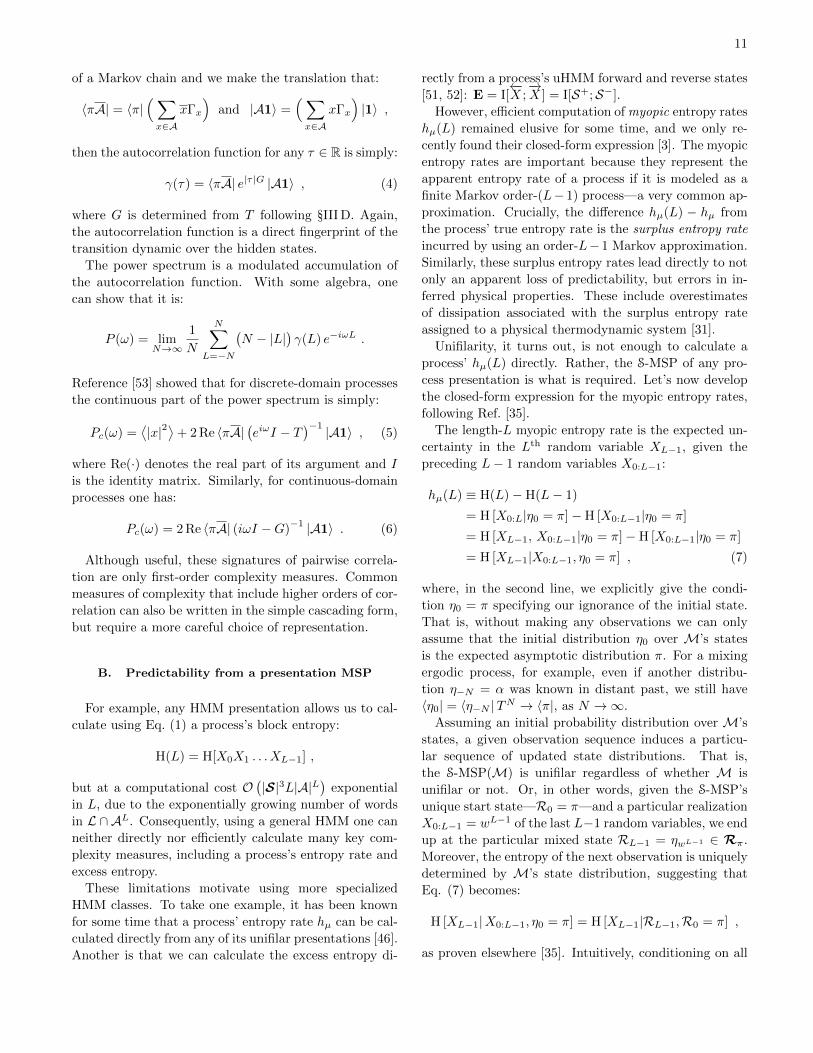
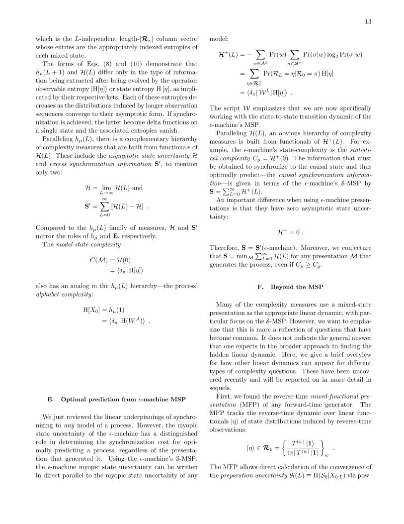
FIG. 1. Example processes generated by the finite HMM classes, depicted by their state-transition diagrams: For any settingof the transition probabilities p, q ∈ (0, 1) and transition rates a, b, c ∈ (0, ∞), each HMM generates an observable stochasticprocess over its alphabet A ⊂ {0, 1, 2}—the latent states themselves are not directly observable from the output process andso are “hidden”. (a) Simple nonunifilar source: Two transitions leaving from the same state generate the same output symbol.(b) Nonminimal unifilar HMM. (c) ε-Machine: Minimal unifilar HMM for the stochastic process generated. (d) Generator of acontinuous-time stochastic process.
the distribution:
〈η010| = 〈π|T (0)T (1)T (0)
〈π|T (0)T (1)T (0) |1〉 .
Since a given observed symbol induces a unique up-
dated distribution from a previous distribution, the dy-
namic over mixed states is unifilar. Transition probabili-
ties among mixed states can be obtained via Eq. (2). So,
if:
〈η|T (x)|1〉 > 0
and:
〈η′| = 〈η|T (x)
〈η|T (x)|1〉 ,
then:
Pr(η′, x|η) = Pr(x|η)
= 〈η|T (x)|1〉 .
These transition probabilities over the mixed states in
Rπ are the matrix elements for the observation-labeled
transition matrices {W (x)}x∈A of M’s synchronizing
MSP (S-MSP):
S-MSP(M) =(Rπ,A, {W (x)}x∈A, δπ
),
where δπ is the distribution over Rπ peaked at the unique
start-(mixed)-state π. The row-stochastic net mixed-
state-to-state transition matrix of S-MSP(M) is W =∑x∈AW
(x). If irreducible, then there is a unique sta-
tionary probability distribution 〈πW | over S-MSP(M)’s
states obtained by solving 〈πW | = 〈πW |W . We useRt to
denote the random variable for the MSP’s state at time
t.
More generally, we must consider a mixed-state dy-
namic that starts from a nonpeaked distribution over the
hidden-state distribution simplex. This may be counter-
intuitive, since a distribution over distributions should
correspond to a single distribution. However, general
MSP theory with a nonpeaked starting distribution over
the simplex allows us to consider a weighted average of
behaviors originating from disparate histories. And, this
is distinct from considering the behavior originating from
a weighted average of histories. This more general MSP
formalism arises in the closed-form solutions for more
sophisticated complexity measures, such as the bound
information. This appears in a sequel.
With this brief overview of mixed states, we can now
turn to use them. Section § V shows that tracking dis-
tributions over the states of another generator makes the
MSP an ideal algebraic object for closed-form complex-
ity expressions involving conditional entropies—measures
that require conditional probabilities. Sections § II B and
§ II C showed that many of the complexity measures for
predictability and predictive burden are indeed framed
as conditional entropies. And so, MSPs are central to
their closed-form expressions.
Historically, mixed states were already implicit in
Ref. [50], introduced in their modern form by Ref. [37,
38], and have been used recently; e.g., in Refs. [51, 52].
Most of these efforts, however, used mixed-states in the
specific context of the synchronizing MSP (S-MSP). A
greatly extended development of mixed-state dynam-
ics appears in Ref. [35]. Different information-theoretic
questions require different mixed-state dynamics, each of
which is a unifilar presentation. Employing the math-
ematical methods developed here, we find that desired
10
closed-form solutions are often simple functions of the
transition dynamic of an appropriate MSP. The spectral
character of the relevant MSP controls the behavior of
information-theoretic quantities.
Finally, we emphasize that similar linear alge-
braic constructions—where hidden states track relevant
information—that are nevertheless not MSPs are just as
important for answering a different set of questions about
a process. Since the other constructions are not directly
about predictability and prediction, we report on these
findings elsewhere.
V. IDENTIFYING THE HIDDEN LINEAR
DYNAMIC
We are now in a position to identify the hidden lin-
ear dynamic appropriate to many of the questions that
arise in complex systems—their observation, predictabil-
ity, prediction, and generation, as outlined in Table II.
In part, this section addresses a very practical need for
specific calculations. In part, it also lays the founda-
tions for further generalizations, to be discussed at the
end. Identifying the linear dynamic means identifying
the linear operator A such that a question of interest can
be reformulated as either being of the cascading form
〈·|An|·〉 or as an accumulation of such cascading events
via 〈·| (∑nAn) |·〉; recall Table I. Helpfully, many well-
known questions of complexity can be mapped to these
archetypal forms. And so, we now proceed to uncover
the hidden linear dynamics of the cascading questions
approximately in the order they were introduced in § II.
A. Simple complexity from any presentation
For observable correlation, any HMM transition opera-
tor will do as the linear dynamic. We simply observe, let
time (or space) evolve forward, and observe again. Let’s
be concrete.
Recall the familiar autocorrelation function. For a
discrete-domain process it is [53]:
γ(L) =⟨XtXt+L
⟩t,
where L ∈ Z and the bar denotes the complex conjugate.
The autocorrelation function is symmetric about L = 0,
so we can focus on L ≥ 0. For L = 0, we simply have:
⟨XtXt
⟩t
=∑
x∈A|x|2 Pr(Xt = x)
=∑
x∈A|x|2 〈π|T (x) |1〉 .
For L > 0, we have:
γ(L) =⟨XtXt+L
⟩t
=∑
x∈A
∑
x′∈Axx′ Pr(Xt = x,Xt+L = x′)
=∑
x∈A
∑
x′∈Axx′ Pr(x ∗ · · · ∗︸ ︷︷ ︸
L−1 ∗sx′)
=∑
x∈A
∑
x′∈Axx′
∑
w∈AL−1
Pr(xwx′) .
Each ‘∗’ above is a wildcard symbol denoting indifference
to the particular symbol observed in its place. That is,
the ∗s denote marginalizing over the intervening random
variables. We develop the consequence of this, explicitly
calculating [54] and finding:
γ(L) =∑
x∈A
∑
x′∈Axx′
∑
w∈AL−1
〈π|T (x)T (w)T (x′) |1〉
=∑
x∈A
∑
x′∈Axx′ 〈π|T (x)
( ∑
w∈AL−1
T (w))T (x′) |1〉
=∑
x∈A
∑
x′∈Axx′ 〈π|T (x)
(L−1∏
i=1
∑
xi∈AT (xi)
︸ ︷︷ ︸=T
)T (x′) |1〉
=∑
x∈A
∑
x′∈Axx′ 〈π|T (x)TL−1T (x′) |1〉
= 〈π|(∑
x∈AxT (x)
)TL−1
( ∑
x′∈Ax′T (x′)
)|1〉 .
The result is the autocorrelation in cascading form
〈·|T t|·〉, which can be made particularly transparent by
subsuming time-independent factors on the left and right
into the bras and kets. Let’s introduce the new row vec-
tor:
〈πA| = 〈π|(∑
x∈AxT (x)
)
and column vector:
|A1〉 =(∑
x∈AxT (x)
)|1〉 .
Then, the autocorrelation function for nonzero integer τ
is simply:
γ(L) = 〈πA|T |L|−1 |A1〉 . (3)
Clearly, the autocorrelation function is a direct, albeit
filtered, signature of iterates of the transition dynamic of
any process presentation.
This result can easily be translated to the continuous-
time setting. If the process is represented as a function
11
of a Markov chain and we make the translation that:
〈πA| = 〈π|(∑
x∈AxΓx
)and |A1〉 =
(∑
x∈AxΓx
)|1〉 ,
then the autocorrelation function for any τ ∈ R is simply:
γ(τ) = 〈πA| e|τ |G |A1〉 , (4)
where G is determined from T following §III D. Again,
the autocorrelation function is a direct fingerprint of the
transition dynamic over the hidden states.
The power spectrum is a modulated accumulation of
the autocorrelation function. With some algebra, one
can show that it is:
P (ω) = limN→∞
1
N
N∑
L=−N
(N − |L|
)γ(L) e−iωL .
Reference [53] showed that for discrete-domain processes
the continuous part of the power spectrum is simply:
Pc(ω) =⟨|x|2⟩
+ 2 Re 〈πA|(eiωI − T
)−1 |A1〉 , (5)
where Re(·) denotes the real part of its argument and I
is the identity matrix. Similarly, for continuous-domain
processes one has:
Pc(ω) = 2 Re 〈πA| (iωI −G)−1 |A1〉 . (6)
Although useful, these signatures of pairwise correla-
tion are only first-order complexity measures. Common
measures of complexity that include higher orders of cor-
relation can also be written in the simple cascading form,
but require a more careful choice of representation.
B. Predictability from a presentation MSP
For example, any HMM presentation allows us to cal-
culate using Eq. (1) a process’s block entropy:
H(L) = H[X0X1 . . . XL−1] ,
but at a computational cost O(|S|3L|A|L
)exponential
in L, due to the exponentially growing number of words
in L ∩AL. Consequently, using a general HMM one can
neither directly nor efficiently calculate many key com-
plexity measures, including a process’s entropy rate and
excess entropy.
These limitations motivate using more specialized
HMM classes. To take one example, it has been known
for some time that a process’ entropy rate hµ can be cal-
culated directly from any of its unifilar presentations [46].
Another is that we can calculate the excess entropy di-
rectly from a process’s uHMM forward and reverse states
[51, 52]: E = I[←−X ;−→X ] = I[S+;S−].
However, efficient computation of myopic entropy rates
hµ(L) remained elusive for some time, and we only re-
cently found their closed-form expression [3]. The myopic
entropy rates are important because they represent the
apparent entropy rate of a process if it is modeled as a
finite Markov order-(L− 1) process—a very common ap-
proximation. Crucially, the difference hµ(L) − hµ from
the process’ true entropy rate is the surplus entropy rate
incurred by using an order-L− 1 Markov approximation.
Similarly, these surplus entropy rates lead directly to not
only an apparent loss of predictability, but errors in in-
ferred physical properties. These include overestimates
of dissipation associated with the surplus entropy rate
assigned to a physical thermodynamic system [31].
Unifilarity, it turns out, is not enough to calculate a
process’ hµ(L) directly. Rather, the S-MSP of any pro-
cess presentation is what is required. Let’s now develop
the closed-form expression for the myopic entropy rates,
following Ref. [35].
The length-L myopic entropy rate is the expected un-
certainty in the Lth random variable XL−1, given the
preceding L− 1 random variables X0:L−1:
hµ(L) ≡ H(L)−H(L− 1)
= H [X0:L|η0 = π]−H [X0:L−1|η0 = π]
= H [XL−1, X0:L−1|η0 = π]−H [X0:L−1|η0 = π]
= H [XL−1|X0:L−1, η0 = π] , (7)
where, in the second line, we explicitly give the condi-
tion η0 = π specifying our ignorance of the initial state.
That is, without making any observations we can only
assume that the initial distribution η0 over M’s states
is the expected asymptotic distribution π. For a mixing
ergodic process, for example, even if another distribu-
tion η−N = α was known in distant past, we still have
〈η0| = 〈η−N |TN → 〈π|, as N →∞.
Assuming an initial probability distribution over M’s
states, a given observation sequence induces a particu-
lar sequence of updated state distributions. That is,
the S-MSP(M) is unifilar regardless of whether M is
unifilar or not. Or, in other words, given the S-MSP’s
unique start state—R0 = π—and a particular realization
X0:L−1 = wL−1 of the last L−1 random variables, we end
up at the particular mixed state RL−1 = ηwL−1 ∈ Rπ.
Moreover, the entropy of the next observation is uniquely
determined by M’s state distribution, suggesting that
Eq. (7) becomes:
H [XL−1|X0:L−1, η0 = π] = H [XL−1|RL−1,R0 = π] ,
as proven elsewhere [35]. Intuitively, conditioning on all

12
of the past observation random variables is equivalent to
conditioning on the random variable for the state distri-
bution induced by particular observation sequences.
We can now recast Eq. (7) in terms of the S-MSP,
finding:
hµ(L) = H [XL−1|RL−1,R0 = π]
=∑
η∈Rπ
Pr(RL−1 = η|R0 = π) H [XL−1|RL−1 = η]
=∑
η∈Rπ
〈δπ|WL−1 |δη〉
× −∑
x∈A〈δη|W (x) |1〉 log2 〈δη|W (x) |1〉
= 〈δπ|WL−1 |H(WA)〉 .
Here:
|H(WA)〉 ≡ −∑
η∈Rπ
|δη〉∑
x∈A〈δη|W (x) |1〉 log2〈δη|W (x) |1〉
is simply the column vector whose ith entry is the entropy
of transitioning from the ith state of S-MSP. Critically,
|H(WA)〉 is independent of L.
Notice that taking the logarithm of the sum of the
entries of the row vector 〈δη|W (x) via 〈δη|W (x) |1〉 is
only permissible since S-MSP’s unifilarity guarantees
that W (x) has at most one nonzero entry per row. (We
also use the familiar convention that 0 log2 0 = 0 [13].)
The result is a particularly compact and efficient ex-
pression for the length-L myopic entropy rates:
hµ(L) = 〈δπ|WL−1 |H(WA)〉 . (8)
Thus, all that is required is computing powers of the MSP
transition dynamic. The computational cost O(L|Rπ|3)
is now only linear in L. Moreover, W is very sparse,
especially so with a small alphabet A. And, this means
that the computational cost can be reduced even further
via numerical optimization.
With hµ(L) in hand, the hierarchy of complexity mea-
sures that derive from it immediately follow, including
the entropy rate hµ, the excess entropy E, and the tran-
sient information T [1]. Specifically, we have:
hµ = limL→∞
hµ(L) ,
E =
∞∑
L=1
[hµ(L)− hµ] , and
T =
∞∑
L=1
L [hµ(L)− hµ] .
The sequel, Part II, discusses these in more detail, intro-
ducing their closed-form expressions. To prepare for this,
we must first review the meromorphic functional calculus,
which is needed for working with the above operators.
C. Continuous time?
We saw that correlation measures are easily ex-
tended to the continuous-time domain via continuous-
time HMMs. Information measures, though, are awk-
ward in continuous time, although progress has been
made recently towards understanding their structure [55,
56].
D. Synchronization from generator MSP
If a process’ state-space is known, then the S-MSP of
the generating model allows one to track the observation-
induced distributions over its states. This naturally leads
to closed-form solutions to informational questions about
how an observer comes to know, or how it synchronizes
to, the system’s states.
To monitor how an observer’s knowledge of a process’
internal state changes with increasing measurements we
use the myopic state uncertainty H(L) = H[S0|X−L:0]
[1]. Expressing it in terms of the S-MSP, one finds [35]:
H(L) = −∑
w∈ALPr(w)
∑
s∈SPr(s|w) log2 Pr(s|w)
=∑
η∈Rπ
Pr(RL = η|R0 = π) H[η] .
Here, H[η] is the presentation-state uncertainty specified
by the mixed state η:
H[η] ≡ −∑
s∈S〈η|δs〉 log2 〈η|δs〉 , (9)
where |δs〉 is the length-|S| column vector of all zeros ex-
cept for a 1 at the appropriate index of the presentation-
state s.
Continuing, we re-express H(L) in terms of powers of
the S-MSP transition dynamic:
H(L) =∑
η∈Rπ
〈δπ|WL |δη〉H [η]
= 〈δπ|WL |H[η]〉 . (10)
Here, we defined:
|H[η]〉 ≡∑
η∈Rπ
|δη〉 H[η] ,
13
which is the L-independent length-|Rπ| column vector
whose entries are the appropriately indexed entropies of
each mixed state.
The forms of Eqs. (8) and (10) demonstrate that
hµ(L + 1) and H(L) differ only in the type of informa-
tion being extracted after being evolved by the operator:
observable entropy |H[η]〉 or state entropy H [η], as impli-
cated by their respective kets. Each of these entropies de-
creases as the distributions induced by longer observation
sequences converge to their asymptotic form. If synchro-
nization is achieved, the latter become delta functions on
a single state and the associated entropies vanish.
Paralleling hµ(L), there is a complementary hierarchy
of complexity measures that are built from functionals of
H(L). These include the asymptotic state uncertainty Hand excess synchronization information S′, to mention
only two:
H = limL→∞
H(L) and
S′ =
∞∑
L=0
[H(L)−H] .
Compared to the hµ(L) family of measures, H and S′
mirror the roles of hµ and E, respectively.
The model state-complexity :
C(M) = H(0)
= 〈δπ |H[η]〉
also has an analog in the hµ(L) hierarchy—the process’
alphabet complexity :
H[X0] = hµ(1)
= 〈δπ |H(WA)〉 .
E. Optimal prediction from ε-machine MSP
We just reviewed the linear underpinnings of synchro-
nizing to any model of a process. However, the myopic
state uncertainty of the ε-machine has a distinguished
role in determining the synchronization cost for opti-
mally predicting a process, regardless of the presenta-
tion that generated it. Using the ε-machine’s S-MSP,
the ε-machine myopic state uncertainty can be written
in direct parallel to the myopic state uncertainty of any
model:
H+(L) = −∑
w∈ALPr(w)
∑
σ∈S+
Pr(σ|w) log2 Pr(σ|w)
=∑
η∈R+π
Pr(RL = η|R0 = π) H[η]
= 〈δπ|WL |H[η]〉 .
The script W emphasizes that we are now specifically
working with the state-to-state transition dynamic of the
ε-machine’s MSP.
Paralleling H(L), an obvious hierarchy of complexity
measures is built from functionals of H+(L). For ex-
ample, the ε-machine’s state-complexity is the statisti-
cal complexity Cµ = H+(0). The information that must
be obtained to synchronize to the causal state and thus
optimally predict—the causal synchronization informa-
tion—is given in terms of the ε-machine’s S-MSP by
S =∑∞L=0H+(L).
An important difference when using ε-machine presen-
tations is that they have zero asymptotic state uncer-
tainty:
H+ = 0 .
Therefore, S = S′(ε-machine). Moreover, we conjecture
that S = minM∑∞L=0H(L) for any presentationM that
generates the process, even if Cµ ≥ Cg.
F. Beyond the MSP
Many of the complexity measures use a mixed-state
presentation as the appropriate linear dynamic, with par-
ticular focus on the S-MSP. However, we want to empha-
size that this is more a reflection of questions that have
become common. It does not indicate the general answer
that one expects in the broader approach to finding the
hidden linear dynamic. Here, we give a brief overview
for how other linear dynamics can appear for different
types of complexity questions. These have been uncov-
ered recently and will be reported on in more detail in
sequels.
First, we found the reverse-time mixed-functional pre-
sentation (MFP) of any forward-time generator. The
MFP tracks the reverse-time dynamic over linear func-
tionals |η〉 of state distributions induced by reverse-time
observations:
|η〉 ∈R1 =
{T (w) |1〉〈π|T (w) |1〉
}
w
.
The MFP allows direct calculation of the convergence of
the preparation uncertainty H(L) ≡ H(S0|X0:L) via pow-

14
ers of the linear MFP transition dynamic. The prepara-
tion uncertainty in turn gives a new perspective on the
transient information since:
T =
∞∑
L=0
(H(S+
0 |X0:L)− χ)
can be interpreted as the predictive advantage of hind-
sight. Related, the myopic process crypticity χ(L) =
H+(L) − H+(L) had been previously introduced [36].
Since limL→∞H+(L) = H+ = 0, the asymptotic cryp-
ticity is χ = H+ +H+ = H+. And, this reveals a refined
partitioning underlying the sum:
∞∑
L=0
(χ− χ(L)
)= S−T ≥ 0 .
Crypticity χ = H(S+0 |X0:∞) itself is positive only if
the process’ cryptic order :
k = min{` ∈ {0, 1, . . . } : H(S+
0 |X−`:∞) = 0},
is positive. The cryptic order is always less than or equal
to its better known cousin, the Markov order R:
R = min{` ∈ {0, 1, . . . } : H(S+
0 |X−`:0) = 0},
since conditioning can never increase entropy. In the
case of cryptic order, we condition on future observations
X0:∞.
The forward-time cryptic operator presentation gives
the forward-time observation-induced dynamic over the
operators:
O ∈{ |s−〉 〈ηw|〈ηw|s−〉 : s− ∈ S−, 〈ηw| ∈Rπ, 〈ηw|s−〉 > 0
}.
Since the reverse causal state S−0 at time 0 is a linear
combination of forward causal states [57, 58], this pre-
sentation allows new calculations of the convergence to
crypticity that implicate Pr(S+0 |X−L:∞).
In fact, the cryptic operator presentation is a special
case of the more general myopic bidirectional dynamic
over operators :
O ∈{|ηw′〉 〈ηw|〈ηw|ηw′〉 : 〈ηw| ∈Rπ, |ηw
′〉 ∈R1, 〈ηw|ηw′〉 > 0
}
induced by new observations of either the future or the
past. This is key to understanding the interplay between
forgetfulness and shortsightedness: Pr(S0|X−M :0, X0:N ).
The list of these extensions continues. Detailed bounds
on entropy-rate convergence are obtained from the transi-
tion dynamic of the so-called possibility machine, beyond
the asymptotic result obtained in Ref. [42]. And, the im-
portance of post-synchronized monitoring, as quantified
by the information lost due to negligence over a duration
`:
bµ(`) = I(X0:`;X`:∞|X−∞:0) ,
can be determined using yet another type of modified
MSP.
These examples all find an exact solution via a the-
ory parallel to that outlined in the following, but applied
to the linear dynamic appropriate for the correspond-
ing complexity question. Furthermore, they highlight the
opportunity, enabled by the full meromorphic functional
calculus [4], to ask and answer more nuanced and, thus,
more probing questions about structure, predictability,
and prediction.
G. The end?
It would seem that we achieved our goal. We identified
the appropriate transition dynamic for common complex-
ity questions and, by some standard, gave formulae for
their exact solution. In point of fact, the effort so far has
all been in preparation. Although we set the framework
up appropriately for linear analysis, closed-form expres-
sions for the complexity measures still await the math-
ematical developments of the following sections. At the
same time, at the level of qualitative understanding and
scientific interpretation, so far we failed to answer the
simple question:
• What range of possible behaviors do these complexity
measures exhibit?
and the natural follow-up question:
• What mechanisms produce qualitatively different in-
formational signatures?
The following section reviews the recently developed
functional calculus that allows us to actually decompose
arbitrary functions of the nondiagonalizable hidden dy-
namic to give conclusive answers to these fundamental
questions [4]. We then analyze the range of possible be-
haviors and identify the internal mechanisms that give
rise to qualitatively different contributions to complex-
ity.
The investment in this and the succeeding sections
allow Part II to express new closed-form solutions for
many complexity measures beyond what those achieved
to date. In addition to obvious calculational advantages,
this also gives new insights into possible behaviors of the
complexity measures and, moreover, their unexpected

15
similarities with each other. In many ways, the results
shed new light on what we were (implicitly) probing with
already-familiar complexity measures. Constructively,
this suggests extending complexity magnitudes to com-
plexity functions that succinctly capture the organization
to all orders of correlation. Just as our intuition for pair-
wise correlation grows out of power spectra, so too these
extensions unveil the workings of both a process’ pre-
dictability and the burden of prediction for an observer.
VI. SPECTRAL THEORY BEYOND THE
SPECTRAL THEOREM
Here, we briefly review the spectral decomposition the-
ory from Ref. [4] needed for working with linear opera-
tors. As will become clear, it goes significantly beyond
the spectral theorem for normal operators.
A. Spectral primer
We restrict our attention to operators that have at
most a countably infinite spectrum. Such operators share
many features with finite-dimensional square matrices.
And so, we review several elementary but essential facts
that are used extensively in the following.
Recall that if A is a finite-dimensional square matrix,
then A’s spectrum is simply its set of eigenvalues:
ΛA ={λ ∈ C : det(λI −A) = 0
},
where det(·) is the determinant of its argument.
For reference later, recall that the algebraic multiplicity
aλ of eigenvalue λ is the power of the term (z−λ) in the
characteristic polynomial det(zI − A). In contrast, the
geometric multiplicity gλ is the dimension of the kernel
of the transformation A − λI or the number of linearly
independent eigenvectors for the eigenvalue. The alge-
braic and geometric multiplicities are all equal when the
matrix is diagonalizable.
Since there can be multiple subspaces associated with
a single eigenvalue, corresponding to different Jordan
blocks in the Jordan canonical form, it is structurally
important to introduce the index of the eigenvalue to
describe the size of its largest-dimension associated sub-
space.
Definition 4. The index νλ of eigenvalue λ is the size
of the largest Jordan block associated with λ.
The index gives information beyond what the algebraic
and geometric multiplicities themselves reveal. Neverthe-
less, for λ ∈ ΛA, it is always true that νλ−1 ≤ aλ−gλ ≤
aλ − 1. In the diagonalizable case, aλ = gλ and νλ = 1
for all λ ∈ ΛA.
The resolvent :
R(z;A) ≡ (zI −A)−1 ,
defined with the help of the continuous complex variable
z ∈ C, captures all of the spectral information about A
through the poles of the resolvent’s matrix elements. In
fact, the resolvent contains more than just the spectrum:
the order of each pole gives the index of the corresponding
eigenvalue.
Each eigenvalue λ of A has an associated projection
operator Aλ, which is the residue of the resolvent as z →λ:
Aλ ≡1
2πi
∮
Cλ
R(z;A)dz . (11)
The residue of the matrix can be calculated elementwise.
The projection operators are orthonormal:
AλAζ = δλ,ζAλ , (12)
and sum to the identity:
I =∑
λ∈ΛA
Aλ . (13)
For cases where νλ = 1, we found that the projection
operator associated with λ can be calculated as [4]:
Aλ =∏
ζ∈ΛAζ 6=λ
(A− ζIλ− ζ
)νζ. (14)
Not all projection operators of a nondiagonalizable op-
erator can be found directly from Eq. (14), since some
have index larger than one. However, if there is only one
eigenvalue that has index larger than one—the almost
diagonalizable case treated in Part II—then Eq. (14), to-
gether with the fact that the projection operators must
sum to the identity, does give a full solution to the set of
projection operators. Next, we consider the general case,
with no restriction on νλ.
B. Eigenprojectors: Left, right, generalized
In general, as we now discuss, an operator’s eigen-
projectors can be obtained from all left and right eigen-
vectors and generalized eigenvectors associated with the
eigenvalue. Given the n-tuple of possibly-degenerate
eigenvalues (ΛA) = (λ1, λ2, . . . , λn), there is a corre-
sponding n-tuple of mk-tuples of linearly-independent
16
generalized right-eigenvectors:
((|λ(m)
1 〉)m1m=1, (|λ(m)
2 〉)m2m=1, . . . , (|λ(m)
n 〉)mnm=1
),
where:
(|λ(m)k 〉)mkm=1 ≡
(|λ(1)k 〉 , |λ
(2)k 〉 , . . . , |λ
(mk)k 〉
)
and a corresponding n-tuple of mk-tuples of linearly-
independent generalized left-eigenvectors:
((〈λ(m)
1 |)m1m=1, (〈λ(m)
2 |)m2m=1, . . . , (〈λ(m)
n |)mnm=1
),
where:
(〈λ(m)k |)mkm=1 ≡
(〈λ(1)k | , 〈λ
(2)k | , . . . , 〈λ
(mk)k |
)
such that:
(A− λkI) |λ(m+1)k 〉 = |λ(m)
k 〉 (15)
and:
〈λ(m+1)k | (A− λkI) = 〈λ(m)
k | , (16)
for 0 ≤ m ≤ mk − 1, where |λ(0)j 〉 = ~0 and 〈λ(0)
j | = ~0.
Specifically, |λ(1)k 〉 and 〈λ(1)
k | are conventional right and
left eigenvectors, respectively.
Recall that eigenvalue λ ∈ ΛA corresponds to gλ differ-
ent Jordan blocks, where gλ is λ’s geometric multiplicity.
In fact:
n =∑
λ∈ΛA
gλ .
Moreover, λ’s index νλ is the size of the largest Jordan
block corresponding to λ:
νλ = max{δλ,λkmk}nk=1 .
Most directly, the generalized right and left eigenvec-
tors can be found as the nontrivial solutions to:
(A− λkI)m |λ(m)k 〉 = |0〉
and:
〈λ(m)k | (A− λkI)m = 〈0| ,
respectively. Imposing appropriate normalization, we
find that:
〈λ(m)j |λ(n)
k 〉 = δj,kδm+n,mk+1 . (17)
Crucially, right and left eigenvectors are no longer
simply related by complex-conjugate transposition and
right eigenvectors are not necessarily orthogonal to each
other. Rather, left eigenvectors and generalized eigenvec-
tors form a dual basis to the right eigenvectors and gen-
eralized eigenvectors. Somewhat surprisingly, the most
generalized left eigenvector 〈λ(mk)k | associated with λk is
dual to the least generalized right eigenvector |λ(1)k 〉 as-
sociated with λk:
〈λ(mk)k |λ(1)
k 〉 = 1 .
Explicitly, we find that the projection operators for a
nondiagonalizable matrix can be written as:
Aλ =
n∑
k=1
mk∑
m=1
δλ,λk |λ(m)k 〉 〈λ(mk+1−m)
k | . (18)
C. Companion operators and resolvent
decomposition
It is useful to introduce the generalized set of compan-
ion operators:
Aλ,m = Aλ(A− λI
)m, (19)
for λ ∈ ΛA and m ∈ {0, 1, 2, . . . }. These operators satisfy
the following semigroup relation:
Aλ,mAζ,n = δλ,ζAλ,m+n . (20)
Aλ,m reduces to the eigenprojector for m = 0:
Aλ,0 = Aλ , (21)
and it exactly reduces to the zero-matrix for m ≥ νλ:
Aλ,m = 0 . (22)
Crucially, we can rewrite the resolvent as a weighted sum
of the companion matrices {Aλ,m}, with complex coef-
ficients that have poles at each eigenvalue λ up to the
eigenvalue’s index νλ:
R(z;A) =∑
λ∈ΛA
νλ−1∑
m=0
1
(z − λ)m+1Aλ,m . (23)
Ultimately these results allow us to evaluate arbitrary
functions of nondiagonalizable operators, to which we
now turn. (Reference [4] gives more background.)
17
D. Functions of nondiagonalizable operators
The meromorphic functional calculus [4] gives meaning
to arbitrary functions f(·) of any linear operator A. Its
starting point is the Cauchy-integral-like formula:
f(A) =∑
λ∈ΛA
1
2πi
∮
Cλ
f(z)R(z;A)dz , (24)
where Cλ denotes a sufficiently small counterclockwise
contour around λ in the complex plane such that no
singularity of the integrand besides the possible pole at
z = λ is enclosed by the contour.
Invoking Eq. (23) yields the desired formulation:
f(A) =∑
λ∈ΛA
νλ−1∑
m=0
Aλ,m1
2πi
∮
Cλ
f(z)
(z − λ)m+1dz . (25)
Hence, with the eigenprojectors {Aλ}λ∈ΛA in hand, eval-
uating an arbitrary function of the nondiagonalizable op-
erator A comes down to the evaluation of several residues.
Typically, evaluating Eq. (25) requires less work than
one might expect when looking at the equation in its full
generality. For example, whenever f(z) is holomorphic
(i.e., well behaved) at z = λ, the residue simplifies to:
1
2πi
∮
Cλ
f(z)
(z − λ)m+1dz =
1
m!f (m)(λ) ,
where f (m)(λ) is the mth derivative of f(z) evaluated at
z = λ. However, if f(z) has a pole or zero at z = λ, then
it substantially changes the complex contour integration.
In the simplest case, when A is diagonalizable and f(z) is
holomorphic at ΛA, the matrix-valued function reduces
to the simple form:
f(A) =∑
λ∈ΛA
f(λ)Aλ .
Moreover, if λ is nondegenerate, then:
Aλ =|λ〉 〈λ|〈λ|λ〉 ,
although 〈λ| here should be interpreted as the solution
to the left eigenequation 〈λ|A = λ 〈λ| and, in general,
〈λ| 6= (|λ〉)†.The meromorphic functional calculus agrees with the
Taylor-series approach whenever the series converges
and agrees with the holomorphic functional calculus of
Ref. [59] whenever f(z) is holomorphic at ΛA. However,
when both these functional calculi fail, the meromorphic
functional calculus extends the domain of f(A) in a way
that is key to the following analysis. We show, for exam-
ple, that within the meromorphic functional calculus, the
negative-one power of a singular operator is the Drazin
inverse. The Drazin inverse effectively inverts everything
that is invertible. Notably, it appears ubiquitously in the
new-found solutions to many complexity measures.
E. Evaluating residues
How does one use Eq. (25)? It says that the spec-
tral decomposition of f(A) reduces to the evaluation of
several residues, where:
Res(g(z), z → λ
)=
1
2πi
∮
Cλ
g(z) dz .
So, to make progress with Eq. (25), we must
evaluate functional-dependent residues of the form
Res(f(z)/(z − λ)m+1, z → λ
). This is basic complex
analysis. Recall that the residue of a complex-valued
function g(z) around its isolated pole λ of order n + 1
can be calculated from:
Res(g(z), z → λ
)=
1
n!limz→λ
dn
dzn[(z − λ)n+1g(z)
].
F. Decomposing AL
Equation (25) allows us to explicitly derive the spectral
decomposition of powers of an operator. For f(A) =
AL → f(z) = zL, z = 0 can be either a zero or a pole
of f(z), depending on the value of L. In either case, an
eigenvalue of λ = 0 will distinguish itself in the residue
calculation of AL via its unique ability to change the
order of the pole (or zero) at z = 0.
For example, at this special value of λ and for integer
L > 0, λ = 0 induces poles that cancel with the zeros of
f(z) = zL, since zL has a zero at z = 0 of order L. For
integer L < 0, an eigenvalue of λ = 0 increases the order
of the z = 0 pole of f(z) = zL. For all other eigenvalues,
the residues will be as expected.
Hence, for any L ∈ C:
AL =
[ ∑
λ∈ΛAλ6=0
νλ−1∑
m=0
(L
m
)λL−mAλ,m
]
+ [0 ∈ ΛA]
ν0−1∑
m=0
δL,mA0Am , (26)

18
where(Lm
)is the generalized binomial coefficient:
(L
m
)=
1
m!
m∏
n=1
(L− n+ 1) , (27)
with(L0
)= 1 and where [0 ∈ ΛA] is the Iverson bracket.
The latter takes value 1 if 0 is an eigenvalue of A and
value 0 if not. Equation (26) applies to any linear oper-
ator with only isolated singularities in its resolvent.
If L is a nonnegative integer such that L ≥ νλ − 1 for
all λ ∈ ΛA, then:
AL =∑
λ∈ΛAλ 6=0
νλ−1∑
m=0
(L
m
)λL−mAλ,m , (28)
where(Lm
)is now reduced to the traditional binomial
coefficient L!/m!(L−m)!.
G. Drazin inverse
The negative-one power of a linear operator is in gen-
eral not the same as the inverse inv(·), since inv(A) need
not exist. However, the negative-one power of a linear
operator is always defined via Eq. (26):
A−1 =∑
λ∈ΛA\{0}
νλ−1∑
m=0
(−1)mλ−1−mAλ,m . (29)
Notably, when the operator is singular, we find that:
AA−1 = I −A0 .
This is the Drazin inverse AD of A, also known as
the {1ν0 , 2, 5}-inverse [60]. (Note that it is not the same
as the Moore–Penrose pseudo-inverse.) Although the
Drazin inverse is usually defined axiomatically to satisfy
certain criteria, here it naturally derived as the nega-
tive one power of a singular operator in the meromorphic
functional calculus.
Whenever A is invertible, however, A−1 = inv(A).
That said, we should not confuse this coincidence with
equivalence. More to the point, there is no reason other
than accidents of historic notation that the negative-one
power should in general be equivalent to the inverse—
especially if an operator is not invertible. To avoid con-
fusing A−1 with inv(A), we use the notation AD for
the Drazin inverse of A. Still, AD = inv(A) whenever
0 /∈ ΛA.
Although Eq. (29) is a constructive way to build the
Drazin inverse, it suggests more work than is actu-
ally necessary. We derived several simple constructions
for it that require only the original operator and the
eigenvalue-0 projector. For example, Ref. [4] found that,
for any c ∈ C \ {0}:
AD = (I −A0)(A+ cA0)−1 . (30)
Later, we will also need the decomposition of (I−W )D,
as it enters into many closed-form complexity expres-
sions. Reference [4] showed that:
(I − T )D = [I − (T − T1)]−1 − T1 (31)
for any stochastic matrix T . If T is the state-transition
matrix of an ergodic process, then the RHS of Eq. (31)
becomes especially simple to evaluate since then T1 =
|1〉 〈π|.Somewhat tangentially, this connects to the fundamen-
tal matrix Z = (I − T + T1)−1 used by Kemeny and
Snell [61] in their analysis of Markovian dynamics. More
immediately, Eq. (31) plays a prominent role when deriv-
ing excess entropy and synchronization information. The
explicit spectral decomposition is also useful:
(I − T )D =∑
λ∈ΛT \{1}
νλ−1∑
m=0
1
(1− λ)m+1Tλ,m . (32)
VII. PROJECTION OPERATORS FOR
STOCHASTIC DYNAMICS
The preceding employed the notation that A is a gen-
eral linear operator. In the following, we reserve T
for the operator of a stochastic transition dynamic, as
in the state-to-state transition dynamic of an HMM:
T =∑x∈A T
(x). If the state space is finite and has a
stationary distribution, then T has a representation that
is a nonnegative row-stochastic—all rows sum to unity—
transition matrix.
We are now in a position to summarize several use-
ful properties for the projection operators of any row-
stochastic matrix T . Naturally, if one uses column-
stochastic instead of row-stochastic matrices, all results
can be translated by simply taking the transpose of ev-
ery line in the derivations. (Recall that (ABC)> =
C>B>A>.)
The transition matrix’s nonnegativity guarantees that
for each λ ∈ ΛT its complex conjugate λ is also in ΛT .
Moreover, the projection operator associated with the
complex conjugate of λ is the complex conjugate of Tλ:
Tλ = Tλ .
If the dynamic induced by T has a stationary distri-
bution over the state space, then T ’s spectral radius is
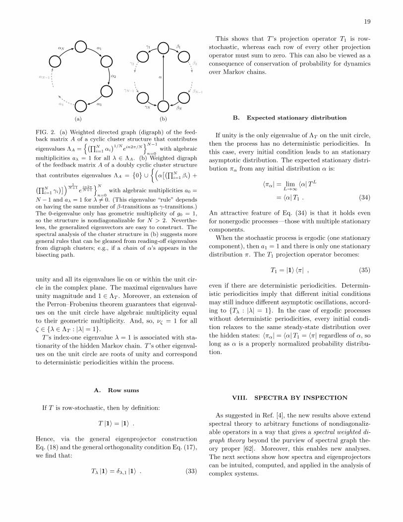
19
↵N ↵1
↵2
↵3↵4
↵N�1
.
↵
�1 �1
�2
�N�1
�N
�N�1
�2
�N
6
(a)
↵N ↵1
↵2
↵3↵4
↵N�1
.
↵
�1 �1
�2
�N�1
�N
�N�1
�2
�N
6
(b)
FIG. 2. (a) Weighted directed graph (digraph) of the feed-back matrix A of a cyclic cluster structure that contributes
eigenvalues ΛA ={(∏N
i=1 αi)1/N
ein2π/N}N−1
n=0with algebraic
multiplicities aλ = 1 for all λ ∈ ΛA. (b) Weighted digraphof the feedback matrix A of a doubly cyclic cluster structure
that contributes eigenvalues ΛA ={
0}∪{(
α[(∏N
i=1 βi)
+
(∏Ni=1 γi
)]) 1N+1
ein2πN+1
}Nn=0
with algebraic multiplicities a0 =
N − 1 and aλ = 1 for λ 6= 0. (This eigenvalue “rule” dependson having the same number of β-transitions as γ-transitions.)The 0-eigenvalue only has geometric multiplicity of g0 = 1,so the structure is nondiagonalizable for N > 2. Neverthe-less, the generalized eigenvectors are easy to construct. Thespectral analysis of the cluster structure in (b) suggests moregeneral rules that can be gleaned from reading-off eigenvaluesfrom digraph clusters; e.g., if a chain of α’s appears in thebisecting path.
unity and all its eigenvalues lie on or within the unit cir-
cle in the complex plane. The maximal eigenvalues have
unity magnitude and 1 ∈ ΛT . Moreover, an extension of
the Perron–Frobenius theorem guarantees that eigenval-
ues on the unit circle have algebraic multiplicity equal
to their geometric multiplicity. And, so, νζ = 1 for all
ζ ∈ {λ ∈ ΛT : |λ| = 1}.T ’s index-one eigenvalue λ = 1 is associated with sta-
tionarity of the hidden Markov chain. T ’s other eigenval-
ues on the unit circle are roots of unity and correspond
to deterministic periodicities within the process.
A. Row sums
If T is row-stochastic, then by definition:
T |1〉 = |1〉 .
Hence, via the general eigenprojector construction
Eq. (18) and the general orthogonality condition Eq. (17),
we find that:
Tλ |1〉 = δλ,1 |1〉 . (33)
This shows that T ’s projection operator T1 is row-
stochastic, whereas each row of every other projection
operator must sum to zero. This can also be viewed as a
consequence of conservation of probability for dynamics
over Markov chains.
B. Expected stationary distribution
If unity is the only eigenvalue of ΛT on the unit circle,
then the process has no deterministic periodicities. In
this case, every initial condition leads to an stationary
asymptotic distribution. The expected stationary distri-
bution πα from any initial distribution α is:
〈πα| = limL→∞
〈α|TL
= 〈α|T1 . (34)
An attractive feature of Eq. (34) is that it holds even
for nonergodic processes—those with multiple stationary
components.
When the stochastic process is ergodic (one stationary
component), then a1 = 1 and there is only one stationary
distribution π. The T1 projection operator becomes:
T1 = |1〉 〈π| , (35)
even if there are deterministic periodicities. Determin-
istic periodicities imply that different initial conditions
may still induce different asymptotic oscillations, accord-
ing to {Tλ : |λ| = 1}. In the case of ergodic processes
without deterministic periodicities, every initial condi-
tion relaxes to the same steady-state distribution over
the hidden states: 〈πα| = 〈α|T1 = 〈π| regardless of α, so
long as α is a properly normalized probability distribu-
tion.
VIII. SPECTRA BY INSPECTION
As suggested in Ref. [4], the new results above extend
spectral theory to arbitrary functions of nondiagonaliz-
able operators in a way that gives a spectral weighted di-
graph theory beyond the purview of spectral graph the-
ory proper [62]. Moreover, this enables new analyses.
The next sections show how spectra and eigenprojectors
can be intuited, computed, and applied in the analysis of
complex systems.
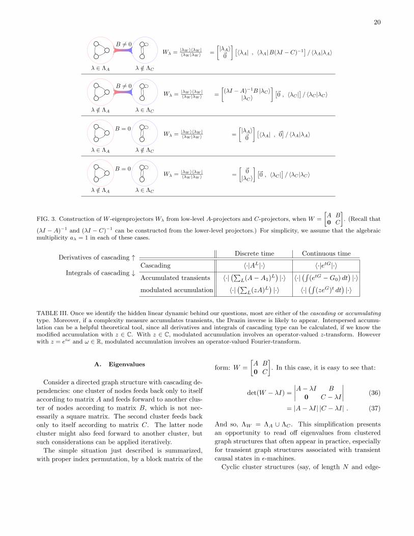
2022
.
.
.
5
� 2 ⇤A � /2 ⇤C
B 6= 0
W� = |�W ih�W |h�W |�W i =
|�Ai~0
� ⇥h�A| , h�A| B(�I � C)�1
⇤/ h�A|�Ai
.
.
.
5
� /2 ⇤A � 2 ⇤C
B 6= 0
W� = |�W ih�W |h�W |�W i =
(�I �A)�1B |�Ci
|�Ci
� ⇥~0 , h�C |
⇤/ h�C |�Ci
.
.
.
5
� 2 ⇤A � /2 ⇤C
B = 0W� = |�W ih�W |
h�W |�W i =
|�Ai~0
� ⇥h�A| , ~0
⇤/ h�A|�Ai
.
.
.
5
� /2 ⇤A � 2 ⇤C
B = 0W� = |�W ih�W |
h�W |�W i =
~0
|�Ci
� ⇥~0 , h�C |
⇤/ h�C |�Ci
FIG. 1: Construction of W -eigenprojectors from ‘lower-level’ A-projectors and C-projectors, when W =
A B0 C
�.
(Recall that (�I �A)�1 and (�I � C)�1 can be constructed from the lower-level projectors.) For simplicity, weassume that the algebraic multiplicity a� = 1 in each of these cases.
necessarily cooperative. XI. SPECTRA BY INSPECTION: USEFUL
RULES FOR WEIGHTED DIGRAPHS
A. Eigenvalues by inspection
B. Eigenprojectors from graph structure
XII. PROJECTION OPERATORS FOR
STOCHASTIC TRANSITION DYNAMICS
Restricting our attention to stochastic state-transition
operators, we are now in a position to elaborate on § VI A
and will derive several useful properties for the projec-
tion operators of any row-stochastic matrix T . Naturally,
if one uses column-stochastic instead of row-stochastic
matrices, all results can be translated by simply taking
the transpose of every line in the derivations—recall that
(ABC)> = C>B>A>.
A. Row Sums: T� |1i = ��,1 |1i
If T is row-stochastic, then by definition:
T |1i = |1i .
Furthermore, clearly the identity matrix is row-
stochastic:
I |1i = |1i .
By the Perron-Frobenius theorem, a row-stochastic tran-
sition matrix always has the eigenvalue of unity with
FIG. 3. Construction of W -eigenprojectors Wλ from low-level A-projectors and C-projectors, when W =
[A B0 C
]. (Recall that
(λI − A)−1 and (λI − C)−1 can be constructed from the lower-level projectors.) For simplicity, we assume that the algebraicmultiplicity aλ = 1 in each of these cases.
Derivatives of cascading ↑
Integrals of cascading ↓
Discrete time Continuous time
Cascading 〈·|AL|·〉 〈·|etG|·〉Accumulated transients 〈·|
(∑L(A−A1)L
)|·〉 〈·|
(∫(etG −G0) dt
)|·〉
modulated accumulation 〈·|(∑
L(zA)L)|·〉 〈·|
(∫(zeG)t dt
)|·〉
TABLE III. Once we identify the hidden linear dynamic behind our questions, most are either of the cascading or accumulatingtype. Moreover, if a complexity measure accumulates transients, the Drazin inverse is likely to appear. Interspersed accumu-lation can be a helpful theoretical tool, since all derivatives and integrals of cascading type can be calculated, if we know themodified accumulation with z ∈ C. With z ∈ C, modulated accumulation involves an operator-valued z-transform. Howeverwith z = eiω and ω ∈ R, modulated accumulation involves an operator-valued Fourier-transform.
A. Eigenvalues
Consider a directed graph structure with cascading de-
pendencies: one cluster of nodes feeds back only to itself
according to matrix A and feeds forward to another clus-
ter of nodes according to matrix B, which is not nec-
essarily a square matrix. The second cluster feeds back
only to itself according to matrix C. The latter node
cluster might also feed forward to another cluster, but
such considerations can be applied iteratively.
The simple situation just described is summarized,
with proper index permutation, by a block matrix of the
form: W =
[A B
0 C
]. In this case, it is easy to see that:
det(W − λI) =
∣∣∣∣A− λI B
0 C − λI
∣∣∣∣ (36)
= |A− λI| |C − λI| . (37)
And so, ΛW = ΛA ∪ ΛC . This simplification presents
an opportunity to read off eigenvalues from clustered
graph structures that often appear in practice, especially
for transient graph structures associated with transient
causal states in ε-machines.
Cyclic cluster structures (say, of length N and edge-
21
weights α1 through αN ) yield especially simple spectra:
ΛA ={( N∏
i=1
αi)1/N
ein2π/N}N−1
n=0. (38)
That is, the eigenvalues are simply the N th roots of the
product of all of the edge-weights. See Fig. 2a.
Similar rules for reading off spectra from other clus-
ter structures exist. Although we cannot list them ex-
haustively here, we give another simple but useful rule in
Fig. 2b. It also indicates the ubiquity of nondiagonaliz-
ability in weighted digraph structures. This second rule
is suggestive of further generalizations where spectra can
be read off from common digraph motifs.
B. Eigenprojectors from graph structure
We just outlined how clustered directed graph struc-
tures yield simplified joint spectra. Is there a corre-
sponding simplification of the projection operators? In
fact, there is and it leads to an iterative construction
of “higher-level” projectors from “lower-level” clustered
components. In contrast to the joint spectrum though,
that completely ignores the feedforward matrix B, the
emergent projectors do require B to pull the associated
eigencontributions into the generalized setting. Figure 3
summarizes the results for the simple case of nondegener-
ate eigenvalues. The general case is constructed similarly.
The preceding results imply a number of algorithms,
both for analytic and numerical calculations. Most di-
rectly, this points to the fact that eigenanalysis can be
partitioned into a series of simpler problems that are
later combined to a final solution. However, in addition
to more efficient serial computation, there are opportu-
nities for numerical parallelization of the algorithms to
compute the eigenprojectors, whether they are computed
directly, say from Eq. (14), or from right and left eigen-
vectors and generalized eigenvectors. Such automation is
useful for applying our analysis to real systems with im-
mense data produced from very high-dimensional state
spaces.
IX. CONCLUSION
Surprisingly, many questions we ask about a structured
stochastic nonlinear process imply a linear dynamic over
a preferred hidden state space. These questions often
concern predictability and prediction. To make predic-
tions about the real world, though, it is not sufficient
to have a model of the world. Additionally, the predic-
tor must synchronize their model to the real-world datathat has been observed up to the present time. This
metadynamic of synchronization—the transition struc-
ture among belief states—is intrinsically linear, but is
typically nondiagonalizable.
Recall the organizational tables from the Introduc-
tion. After all of the intervening detail, let’s consider
a more nuanced formulation. We saw that once we
frame our questions in terms of the hidden linear transi-
tion dynamic, complexity measures are usually either of
the cascading or accumulation type. Scalar complexity
measures often accumulate only the interesting transient
structure that rides on top of the asymptotics. Skimming
off the asymptotics led to a Drazin inverse. Modified
accumulation turns complexity scalars into complexity
functions. This is summarized in Table III and Table IV.
It is notable that Table IV gives closed-form formulae
for many complexity measures that previously were only
expressed as infinite sums over functions of probabilities.
Let us remind ourselves: Why, in this analysis, were
nondiagonalizable dynamics noteworthy? They are note-
worthy since the metadynamics of diagonalizable dynam-
ics are generically nondiagonalizable—typically due to
the zero-eigenvalue subspace that is responsible for the
initial, ephemeral epoch of symmetry collapse. We saw
this explicitly with the metadynamics of transitioning be-
tween belief states. However, other metadynamics be-
yond that focused on prediction are also generically non-
diagonalizable. For example, in the analysis of quan-
tum compression, crypticity, and other aspects of hidden
structure, the relevant linear dynamic is not the MSP,
but is nevertheless a nondiagonalizable structure that is
fruitfully analyzed with the recently generalized spectral
theory of nonnormal operators [4].
Using the appropriate dynamic for common complex-
ity questions and the meromorphic functional calculus
to overcome nondiagonalizability, the sequel (Part II)
goes on to develop closed-form expressions for complexity
measures as simple functions of the corresponding tran-
sition dynamic of the implied HMM.
ACKNOWLEDGMENTS
JPC thanks the Santa Fe Institute for its hospitality.
The authors thank Chris Ellison, Ryan James, John Ma-
honey, Alec Boyd, and Dowman Varn for helpful discus-
sions. This material is based upon work supported by,
or in part by, the U. S. Army Research Laboratory and
the U. S. Army Research Office under contract numbers
W911NF-12-1-0234, W911NF-13-1-0340, and W911NF-
13-1-0390.

22
22
Derivatives of cascading "
Integrals of cascading #
Discrete time Continuous time
Cascading h·|AL|·i h·|etG|·iAccumulated transients h·|
�PL(A�A1)
L�|·i h·|
�R(etG �G0) dt
�|·i
modulated accumulation h·|�P
L(zA)L�|·i h·|
�R(zeG)t dt
�|·i
TABLE III. Once we identify the hidden linear dynamic behind our questions, most questions we tend to ask are either ofthe cascading or accumulating type. If a complexity measure accumulates transients, the Drazin inverse is likely to appear.Interspersed accumulation can be a nice theoretical tool, since all derivatives and integrals of cascading can be calculated if weknow the modified accumulation with z 2 C. With z 2 C, modulated accumulation involves an operator-valued z-transform.With z = ei! and ! 2 R, modulated accumulation involves an operator-valued Fourier-transform.
GenreImplied linear
transition dynamic
Example QuestionsCascading Accumulated transients Modulated accumulation
Overt
Observational
Transition matrix T
of any HMM
Correlations, �(L):
h⇡A| T |L|�1 |A1iGreen–Kubo
transport coe�cients
Power spectra, P (!):
2R h⇡A|�ei!I � T
��1 |A1i
PredictabilityTransition matrix W
of MSP of any HMM
Myopic entropy rate, hµ(L):
h�⇡| W L�1 |H(W A)iExcess entropy, E:
h�⇡| (I � W )D |H(W A)iE(z):
h�⇡| (zI � W )�1 |H(W A)iOptimal
Prediction
Transition matrix Wof MSP of ✏-machine
Causal state uncertainty, H+(L):
h�⇡| WL |H[⌘]iSynchronization info, S:
h�⇡| (I � W)D |H[⌘]iS(z):
h�⇡| (zI � W)�1 |H[⌘]i...
......
......
TABLE IV. Several genres of questions about the complexity of a process are given in the left column of the table in order ofincreasing sophistication. Each genre implies a di↵erent linear transition dynamic. Closed-form formulae are given for examplecomplexity measures, showing the deep similarity among formulae of the same column, while formulae in the same row havematching bra-ket pairs. The similarity within the column corresponds to similarity in the type of time-evolution implied bythe question type. The similarity within the row corresponds to similarity in the genre of the question.
ACKNOWLEDGMENTS
JPC thanks the Santa Fe Institute for its hospital-
ity. The authors thank Chris Ellison, Ryan James, and
Dowman Varn for helpful discussions. This material is
based upon work supported by, or in part by, the U. S.
Army Research Laboratory and the U. S. Army Research
O�ce under contract numbers W911NF-12-1-0234 and
W911NF-13-1-0390.
[1] J. P. Crutchfield, P. M. Riechers, and C. J. Ellison. Exact
complexity: Spectral decomposition of intrinsic compu-
tation. submitted. Santa Fe Institute Working Paper
13-09-028; arXiv:1309.3792 [cond-mat.stat-mech]. 2
[2] P. M. Riechers, J. R. Mahoney, C. Aghamohammadi,
and J. P. Crutchfield. A closed-form shave from occam’s
quantum razor: Exact results for quantum compression.
submitted. arXiv:1510.08186 [quant-ph]. 2
[3] P. M. Riechers and J. P. Crutchfield. Broken reversibility:
Fluctuation theorems and exact results for the thermo-
dynamics of complex nonequilibrium systems. in prepa-
ration. 2
[4] J. P. Crutchfield. Between order and chaos. Nature
Physics, 8(January):17–24, 2012. 3, 4, 6
[5] J. J. Binney, N. J. Dowrick, A. J. Fisher, and M. E. J.
Newman. The Theory of Critical Phenomena. Oxford
University Press, Oxford, 1992. 3
[6] J. P. Crutchfield and D. P. Feldman. Regularities un-
seen, randomness observed: Levels of entropy conver-
gence. CHAOS, 13(1):25–54, 2003. 3, 4, 9
[7] T. M. Cover and J. A. Thomas. Elements of Information
Theory. Wiley-Interscience, New York, second edition,
2006. 3, 9
[8] A. N. Kolmogorov. Entropy per unit time as a metric
invariant of automorphisms. Dokl. Akad. Nauk. SSSR,
124:754, 1959. (Russian) Math. Rev. vol. 21, no. 2035b.
4
[9] J. P. Crutchfield and D. P. Feldman. Synchronizing to
the environment: Information theoretic limits on agent
learning. Adv. in Complex Systems, 4(2):251–264, 2001.
4
TABLE IV. Genres of complexity questions given in order of increasing sophistication; summary of Part I and a preview of PartII. Each implies a different linear transition dynamic. Closed-form formulae are given for several complexity measures, showingthe similarity among them down the same column. Formulae in the same row have matching bra-ket pairs. The similaritywithin the column corresponds to similarity in the time-evolution implied by the question type. The similarity within the rowcorresponds to similarity in question genre.
[1] J. P. Crutchfield and D. P. Feldman. Regularities un-
seen, randomness observed: Levels of entropy conver-
gence. CHAOS, 13(1):25–54, 2003. 2, 4, 5, 6, 12
[2] S. E. Marzen and J. P. Crutchfield. Nearly maximally
predictive features and their dimensions. Phys. Rev. E,
in press, 2017. arxiv.org:1702.08565]. 2, 5
[3] J. P. Crutchfield, C. J. Ellison, and P. M. Riechers. Ex-
act complexity: The spectral decomposition of intrinsic
computation. Phys. Lett. A, 380(9):998–1002, 2016. 2, 3,
11
[4] P. M. Riechers and J. P. Crutchfield. Beyond the spectral
theorem: Decomposing arbitrary functions of nondiago-
nalizable operators. arxiv.org:1607.06526. 2, 3, 14, 15,
16, 17, 18, 19, 21
[5] While we follow Shannon [12] in this, it differs from the
more widely used state-labeled HMMs. 2
[6] C. Moore and J. P. Crutchfield. Quantum automata and
quantum grammars. Theoret. Comp. Sci., 237:1-2:275–
306, 2000. 2
[7] L. A. Clark, W. Huang, T. M. Barlow, and A. Beige. Hid-
den quantum markov models and open quantum systems
with instantaneous feedback. New. J. Phys., 14:143–151,
2015. 2
[8] O. Penrose. Foundations of statistical mechanics; a de-
ductive treatment. Pergamon Press, Oxford, 1970. 2
[9] U. Seifert. Stochastic thermodynamics, fluctuation the-
orems and molecular machines. Rep. Prog. Phys.,
75:126001, 2012. 2
[10] R. Klages, W. Just, and C. Jarzynski, editors. Nonequi-
librium Statistical Physics of Small Systems: Fluctuation
Relations and Beyond. Wiley, New York, 2013.
[11] J. Bechhoefer. Hidden Markov models for stochastic ther-
modynamics. New. J. Phys., 17:075003, 2015. 2
[12] C. E. Shannon. A mathematical theory of communica-
tion. Bell Sys. Tech. J., 27:379–423, 623–656, 1948. 2,
22
[13] T. M. Cover and J. A. Thomas. Elements of Information
Theory. Wiley-Interscience, New York, second edition,
2006. 2, 4, 7, 12, 23
[14] L. R. Rabiner and B. H. Juang. An introduction to hid-
den Markov models. IEEE ASSP Magazine, January,
1986. 2
[15] R. A. Roberts and C. T. Mullis. Digital Signal Processing.
Addison-Wesley, Reading, Massachusetts, 1987.
[16] L. R. Rabiner. A tutorial on hidden Markov models and
selected applications. IEEE Proc., 77:257, 1989. 2
[17] M. O. Rabin. Probabilistic automata. Info. Control,
6:230–245, 1963. 2
[18] W. J. Ewens. Mathematical Population Genetics.
Springer, New York, second edition, 2004. 2
[19] M. Nowak. Evolutionary Dynamics: Exploring the Equa-
tions of Life. Belnap Press, New York, 2006. 2
[20] J. P. Crutchfield. Between order and chaos. Nature
Physics, 8(January):17–24, 2012. 3, 5, 7
[21] P. Stoica and R. L. Moses. Spectral Analysis of Signals.
Pearson Prentice Hall, Upper Saddle River, New Jersey,
2005. 4
[22] R. W. Hamming. Digital Filterns. Dover Publications,
New York, third edition, 1997. 4
[23] M M. Woolfson. An Introduction to X-ray Crystallog-
raphy. Cambridge University Press, Cambridge, United
Kingdom, 1997. 4
[24] M. S. Green. Markoff random processes and the statis-
tical mechanics of time-dependent phenomena. II. Irre-
versible processes in fluids. J. Chem. Physics, 22(3):398–
413, 1954. 4
[25] R. Zwanzig. Time-correlation functions and transport co-
efficients in statistical mechanics. Ann. Rev. Phys. Chem-
istry, 16(1):67–102, 1965. 4
[26] J. J. Binney, N. J. Dowrick, A. J. Fisher, and M. E. J.
Newman. The Theory of Critical Phenomena. Oxford
University Press, Oxford, 1992. 4
23
[27] A. N. Kolmogorov. Entropy per unit time as a metric
invariant of automorphisms. Dokl. Akad. Nauk. SSSR,
124:754, 1959. (Russian) Math. Rev. vol. 21, no. 2035b.
4
[28] R. G. James, C. J. Ellison, and J. P. Crutchfield.
Anatomy of a bit: Information in a time series obser-
vation. CHAOS, 21(3):037109, 2011. 5
[29] P. M. Ara, R. G. James, and J. P. Crutchfield. The
elusive present: Hidden past and future dependence and
why we build models. Phys. Rev. E, 93(2):022143, 2016.
5
[30] J. P. Crutchfield and K. Young. Inferring statistical com-
plexity. Phys. Rev. Let., 63:105–108, 1989. 5
[31] A. B. Boyd, D. Mandal, and J. P. Crutchfield. Leverag-
ing environmental correlations: The thermodynamics of
requisite variety. J. Stat. Phys., 167(6):1555–1585, 2016.
5, 11
[32] S. Still, J. P. Crutchfield, and C. J. Ellison. Optimal
causal inference: Estimating stored information and ap-
proximating causal architecture. CHAOS, 20(3):037111,
2010. 5
[33] F. Creutzig, A. Globerson, and N. Tishby. Past-future
information bottleneck in dynamical systems. Phys. Rev.
E, 79(4):041925, 2009.
[34] S. E. Marzen and J. P. Crutchfield. Predictive rate-
distortion for infinite-order Markov processes. J. Stat.
Phys., 163(6):1312–1338, 2016. 5
[35] C. J. Ellison and J. P. Crutchfield. States of states of
uncertainty. in preparation. 5, 9, 11, 12
[36] J. R. Mahoney, C. J. Ellison, R. G. James, and J. P.
Crutchfield. How hidden are hidden processes? a
primer on crypticity and entropy convergence. CHAOS,
21(3):037112, 2011. 6, 14
[37] J. P. Crutchfield. The calculi of emergence: Compu-
tation, dynamics, and induction. Physica D, 75:11–54,
1994. 6, 8, 9
[38] D. R. Upper. Theory and Algorithms for Hidden Markov
Models and Generalized Hidden Markov Models. PhD
thesis, University of California, Berkeley, 1997. Published
by University Microfilms Intl, Ann Arbor, Michigan. 9,
23
[39] W. Lohr and N. Ay. Non-sufficient memories that are
sufficient for prediction. In Complex Sciences, volume 4
of Lecture Notes of the Institute for Computer Sciences,
Social Informatics and Telecommunications Engineering,
pages 265–276. 2009. 6
[40] J. P. Crutchfield, C. J. Ellison, J. R. Mahoney, and R. G.
James. Synchronization and control in intrinsic and de-
signed computation: An information-theoretic analysis
of competing models of stochastic computation. CHAOS,
20(3):037105, 2010. 6
[41] N. Travers and J. P. Crutchfield. Exact synchronization
for finite-state sources. J. Stat. Phys., 145(5):1181–1201,
2011. 6, 7
[42] N. Travers and J. P. Crutchfield. Asymptotic syn-
chronization for finite-state sources. J. Stat. Phys.,
145(5):1202–1223, 2011. 6, 7, 14
[43] J. R. Mahoney, C. Aghamohammadi, and J. P. Crutch-
field. Occam’s quantum strop: Synchronizing and com-
pressing classical cryptic processes via a quantum chan-
nel. Scientific Reports, 6:20495, 2016. 6
[44] Contrast this with the class-equivalent state-labeled
HMMs, also known as Moore HMMs [38, 63, 64]. In au-
tomata theory, a finite-state HMM is called a probabilistic
nondeterministic finite automaton [65]. Information the-
ory [13] refers to them as finite-state information sources.
And, stochastic process theory defines them as functions
of a Markov chain [46, 50, 66, 67]. 6
[45] P. A. M. Dirac. A new notation for quantum mechanics.
Math. Proc. Cambridge Phil. Soc., 35(3):416–418, 1939.
6
[46] R. B. Ash. Information Theory. Dover Books on Ad-
vanced Mathematics. Dover Publications, 1965. 7, 11,
23
[47] C. R. Shalizi and J. P. Crutchfield. Computational me-
chanics: Pattern and prediction, structure and simplicity.
J. Stat. Phys., 104:817–879, 2001. 7
[48] Automata theory would refer to a uHMM as a proba-
bilistic deterministic finite automaton [65]. The awkward
terminology does not recommend itself. 7
[49] J. E. Hopcroft and J. D. Ullman. Introduction to Au-
tomata Theory, Languages, and Computation. Addison-
Wesley, Reading, 1979. 7
[50] D. Blackwell. The entropy of functions of finite-state
Markov chains. volume 28, pages 13–20, Publishing
House of the Czechoslovak Academy of Sciences, Prague,
1957. 9, 23
[51] J. P. Crutchfield, C. J. Ellison, and J. R. Mahoney.
Time’s barbed arrow: Irreversibility, crypticity, and
stored information. Phys. Rev. Lett., 103(9):094101,
2009. 9, 11
[52] C. J. Ellison, J. R. Mahoney, and J. P. Crutchfield.
Prediction, retrodiction, and the amount of information
stored in the present. J. Stat. Phys., 136(6):1005–1034,
2009. 9, 11
[53] P. M. Riechers and J. P. Crutchfield. Power spectra of
stochastic processes from transition matrices of hidden
Markov models. in preparation. 10, 11
[54] Averaging over t invokes unconditioned word probabili-
ties that must be calculated using the stationary proba-
bility π over the recurrent states. Effectively this ignores
any transient nonstationarity that may exist in a process,
since only the recurrent part of the HMM presentation
plays a role in the autocorrelation function. One practi-
cal lesson is that if T has transient states, they might as
well be trimmed prior to such a calculation. 10
[55] S. Marzen, M. R. DeWeese, and J. P. Crutchfield. Time
resolution dependence of information measures for spik-
ing neurons: Scaling and universality. Front. Comput.
Neurosci., 9:109, 2015. 12
[56] S. Marzen and J. P. Crutchfield. Informational and causal
architecture of continuous-time renewal processes. J.
Stat. Phys., in press, 2017. arxiv.org:1611.01099. 12
[57] J. R. Mahoney, C. J. Ellison, and J. P. Crutchfield. In-
formation accessibility and cryptic processes. J. Phys. A:

24
Math. Theo., 42:362002, 2009. 14
[58] J. R. Mahoney, C. J. Ellison, and J. P. Crutchfield. Infor-
mation accessibility and cryptic processes: Linear combi-
nations of causal states. arxiv.org:0906.5099 [cond-mat].
14
[59] N. Dunford. Spectral theory I. Convergence to projec-
tions. Trans. Am. Math. Soc., 54(2):pp. 185–217, 1943.
17
[60] A. Ben-Israel and T.N.E. Greville. Generalized Inverses:
Theory and Applications. CMS Books in Mathematics.
Springer, 2003. 18
[61] J. G. Kemeny and J. L. Snell. Finite Markov chains,
volume 356. Springer, New York, 1960. 18
[62] D. M. Cvetkovic, M. Doob, and H. Sachs. Spectra of
Graphs: Theory and Applications. Wiley, New York, New
York, third edition, 1998. 19
[63] V. Balasubramanian. Equivalence and reduction of hid-
den Markov models. Technical Report AITR-1370, 1993.
23
[64] B. Vanluyten, J. C. Willems, and B. De Moor. Equiva-
lence of state representations for hidden Markov models.
Systems & Control Letters, 57(5):410 – 419, 2008. 23
[65] M. Sipser. Introduction to the Theory of Computation.
Cengage Learning, 2012. 23
[66] J. J. Birch. Approximations for the entropy for functions
of Markov chains. Ann. Math. Statist., 33(2):930–938,
1962. 23
[67] N. F. Travers. Exponential bounds for convergence of
entropy rate approximations in hidden markov models
satisfying a path-mergeability condition. Stochastic Pro-
cesses and their Applications, 124(12):4149–4170, 2014.
23