spectral analysis with the dft - university of california ...ee123/fa12/notes/lecture07.pdf · key...

Fall 2011, EE123 Digital Signal Processing

Lecture 7 (chap 10.1-10.2)

Miki Lustig, UCB

September 13, 2012

Miki Lustig, UCB Fall 2011, EE123 Digital Signal Processing

Spectral Analysis with the DFT

The DFT can be used to analyze the spectrum of a signal.

It would seem that this should be simple, take a block of the signaland compute the spectrum with the DFT.

However, there are many important issues and tradeo↵s:

Signal duration vs spectral resolutionSignal sampling rate vs spectral rangeSpectral sampling rateSpectral artifacts

Miki Lustig UCB. Based on Course Notes by J.M Kahn Fall 2011, EE123 Digital Signal Processing


Consider these steps of processing continuous-time signals:



Two important tools:

Applying a window to the input signal – reduces spectralartifactsPadding input signal with zeros – increases the spectralsampling

Key Parameters:

Parameter Symbol Units

Sampling interval T sSampling frequency !

s

= 2⇡T

rad/sWindow length L unitlessWindow duration L · T sDFT length N � L unitlessDFT duration N · T sSpectral resolution !

s

L

= 2⇡L·T rad/s

Spectral sampling interval !s

N

= 2⇡N·T rad/s


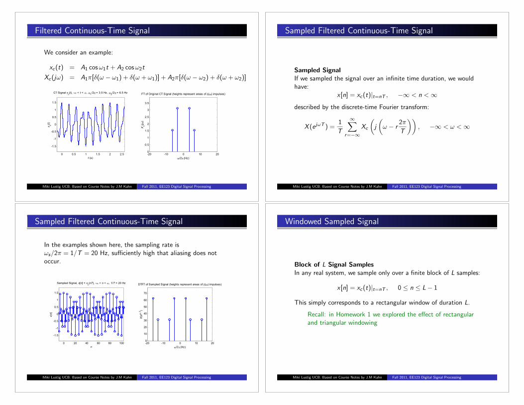
Filtered Continuous-Time Signal

We consider an example:

x

c

(t) = A

1

cos!1

t + A

2

cos!2

t

X

c

(j!) = A

1

⇡[�(! � !1

) + �(! + !1

)] + A

2

⇡[�(! � !2

) + �(! + !2

)]

0 0.5 1 1.5 2 2.5

-1.5

-1

-0.5

0

0.5

1

1.5

t (s)

x c(t

)

CT Signal xc(t), - < t < ,

1/2 = 3.5 Hz,

2/2 = 6.5 Hz

-20 -10 0 10 200

0.5

1

1.5

2

2.5

3

3.5

/2 (Hz)

Xc(j

)

FT of Original CT Signal (heights represent areas of ( ) impulses)


Sampled Filtered Continuous-Time Signal

Sampled SignalIf we sampled the signal over an infinite time duration, we wouldhave:

x [n] = x

c

(t)|t=nT

, �1 < n < 1

described by the discrete-time Fourier transform:

X (e j!T ) =1

T

1X

r=�1X

c

✓j

✓! � r

2⇡

T

◆◆, �1 < ! < 1


Sampled Filtered Continuous-Time Signal

In the examples shown here, the sampling rate is!s

/2⇡ = 1/T = 20 Hz, su�ciently high that aliasing does notoccur.

0 20 40 60 80 100

-1.5

-1

-0.5

0

0.5

1

1.5

n

x[n

]

Sampled Signal, x[n] = xc(nT), - < n < , 1/T = 20 Hz

-20 -10 0 10 200

10

20

30

40

50

60

70

/2 (Hz)

X(ejT)

DTFT of Sampled Signal (heights represent areas of ( ) impulses)


Windowed Sampled Signal

Block of L Signal SamplesIn any real system, we sample only over a finite block of L samples:

x [n] = x

c

(t)|t=nT

, 0 n L� 1

This simply corresponds to a rectangular window of duration L.

Recall: in Homework 1 we explored the e↵ect of rectangularand triangular windowing



Windowed Block of L Signal SamplesWe take the block of signal samples and multiply by a window ofduration L, obtaining:

v [n] = x [n] · w [n], 0 n L� 1

Suppose the window w [n] has DTFT W (e j!T ).

Then the windowed block of signal samples has a DTFT given bythe periodic convolution between X (e j!T ) and W (e j!T ):

V (e j!T ) =1

2⇡

Z ⇡

�⇡X (e j✓)W (e j(!T�✓))d✓



Convolution with W (e j!T ) has two e↵ects in the spectrum:

1 It limits the spectral resolution. – Main lobes of the DTFT ofthe window

2 The window can produce spectral leakage. – Side lobes of theDTFT of the window

* These two are always a tradeo↵ - time-frequency uncertaintyprinciple


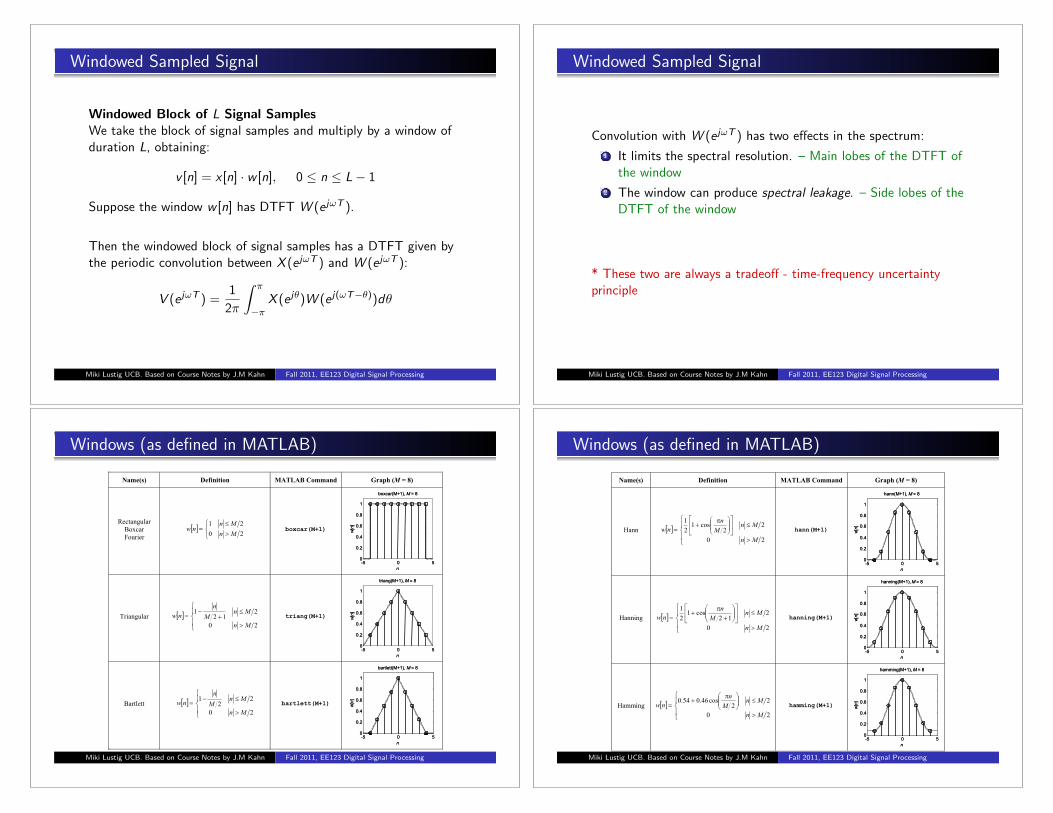
Windows (as defined in MATLAB)

-5 0 50

0.2

0.4

0.6

0.8

1

n

w[n

]

boxcar(M+1), M = 8

-5 0 50

0.2

0.4

0.6

0.8

1

n

w[n

]

boxcar(M+1), M = 8

-5 0 50

0.2

0.4

0.6

0.8

1

n

w[n

]

triang(M+1), M = 8

-5 0 50

0.2

0.4

0.6

0.8

1

n

w[n

]

triang(M+1), M = 8

-5 0 50

0.2

0.4

0.6

0.8

1

n

w[n

]

bartlett(M+1), M = 8

-5 0 50

0.2

0.4

0.6

0.8

1

n

w[n

]

bartlett(M+1), M = 8

Name(s) Definition MATLAB Command Graph (M = 8)

Rectangular

Boxcar

Fourier

nw20

21

Mn

Mnboxcar(M+1)

Triangular nw

20

212

1

Mn

MnM

n

triang(M+1)

Bartlett nw

20

22

1

Mn

MnM

n

bartlett(M+1)


Windows (as defined in MATLAB)

-5 0 50

0.2

0.4

0.6

0.8

1

n

w[n

]

hann(M+1), M = 8

-5 0 50

0.2

0.4

0.6

0.8

1

n

w[n

]

hann(M+1), M = 8

-5 0 50

0.2

0.4

0.6

0.8

1

n

w[n

]

hanning(M+1), M = 8

-5 0 50

0.2

0.4

0.6

0.8

1

n

w[n

]

hanning(M+1), M = 8

-5 0 50

0.2

0.4

0.6

0.8

1

n

w[n

]

hamming(M+1), M = 8

-5 0 50

0.2

0.4

0.6

0.8

1

n

w[n

]

hamming(M+1), M = 8

Name(s) Definition MATLAB Command Graph (M = 8)

Hann nw

20

22

cos12

1

Mn

MnM

n

hann(M+1)

Hanning nw

20

212

cos12

1

Mn

MnM

n

hanning(M+1)

Hamming nw

20

22

cos46.054.0

Mn

MnM

n

hamming(M+1)


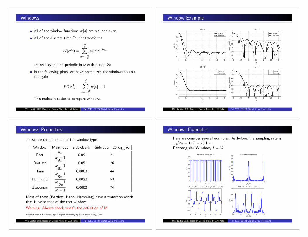
Windows

All of the window functions w [n] are real and even.

All of the discrete-time Fourier transforms

W (e j!) =

M

2X

n=�M

2

w [n]e�jn!

are real, even, and periodic in ! with period 2⇡.

In the following plots, we have normalized the windows to unitd.c. gain:

W (e j0) =

M

2X

n=�M

2

w [n] = 1

This makes it easier to compare windows.


Window Example

0 0.5 1 1.5 2 2.5 3

-0.2

0

0.2

0.4

0.6

0.8

1

W(ej

)

M = 16

Boxcar

Triangular

0 0.5 1 1.5 2 2.5 3

-0.2

0

0.2

0.4

0.6

0.8

1

W(ej

)

M = 16

Hanning

Hamming

0 0.5 1 1.5 2 2.5 3-70

-60

-50

-40

-30

-20

-10

0

20

lo

g1

0|W

(ej

)|

M = 16

Boxcar

Triangular

0 0.5 1 1.5 2 2.5 3-70

-60

-50

-40

-30

-20

-10

0

20

lo

g1

0|W

(ej

)|

M = 16

Hanning

Hamming


Windows Properties

These are characteristic of the window type

Window Main-lobe Sidelobe �s

Sidelobe �20 log10

�s

Rect4⇡

M + 10.09 21

Bartlett8⇡

M + 10.05 26

Hann8⇡

M + 10.0063 44

Hamming8⇡

M + 10.0022 53

Blackman12⇡

M + 10.0002 74

Most of these (Bartlett, Hann, Hamming) have a transition widththat is twice that of the rect window.

Warning: Always check what’s the definition of M

Adapted from A Course In Digital Signal Processing by Boaz Porat, Wiley, 1997


Windows Examples

Here we consider several examples. As before, the sampling rate is!s

/2⇡ = 1/T = 20 Hz.Rectangular Window, L = 32

0 5 10 15 20 25 300

0.2

0.4

0.6

0.8

1

1.2

n

w[n

]

Rectangular Window, L = 32

-20 -10 0 10 200

5

10

15

20

25

30

35

40

/2 (Hz)

|W(ejT)|

DTFT of Rectangular Window

0 5 10 15 20 25 30

-1.5

-1

-0.5

0

0.5

1

1.5

n

v[n

]Sampled, Windowed Signal, Rectangular Window, L = 32

-20 -10 0 10 200

5

10

15

20

/2 (Hz)

|V(ejT)|

DTFT of Sampled, Windowed Signal


Windows Examples

Triangular Window, L = 32

0 5 10 15 20 25 300

0.2

0.4

0.6

0.8

1

1.2

n

w[n

]Triangular Window, L = 32

-20 -10 0 10 200

5

10

15

20

/2 (Hz)

|W(ejT)|

DTFT of Triangular Window

0 5 10 15 20 25 30

-1.5

-1

-0.5

0

0.5

1

1.5

n

v[n

]

Sampled, Windowed Signal, Triangular Window, L = 32

-20 -10 0 10 200

2

4

6

8

/2 (Hz)

|V(ejT)|



Windows Examples

Hamming Window, L = 32

0 5 10 15 20 25 300

0.2

0.4

0.6

0.8

1

1.2

n

w[n

]


-20 -10 0 10 200

5

10

15

20

/2 (Hz)

|W(ejT)|

DTFT of Hamming Window

0 5 10 15 20 25 30

-1.5

-1

-0.5

0

0.5

1

1.5

n

v[n

]

Sampled, Windowed Signal, Hamming Window, L = 32

-20 -10 0 10 200

2

4

6

8

10

/2 (Hz)

|V(ejT)|



Windows Examples


0 10 20 30 40 50 600

0.2

0.4

0.6

0.8

1

1.2

n

w[n

]


-20 -10 0 10 200

5

10

15

20

25

30

35

40

/2 (Hz)

|W(ejT)|

DTFT of Hamming Window

0 10 20 30 40 50 60

-1.5

-1

-0.5

0

0.5

1

1.5

n

v[n

]

Sampled, Windowed Signal, Hamming Window, L = 64

-20 -10 0 10 200

5

10

15

20

/2 (Hz)

|V(ejT)|



Zero-Padding

In preparation for taking an N-point DFT, we may zero-padthe windowed block of signal samples to a block length N � L:

(v [n] 0 n L� 1

0 L n N � 1

This zero-padding has no e↵ect on the DTFT of v [n], sincethe DTFT is computed by summing over �1 < n < 1.

E↵ect of Zero Padding

We take the N-point DFT of the zero-padded v [n], to obtainthe block of N spectral samples:

V [k], 0 k N � 1


Zero-Padding

Consider the DTFT of the zero-padded v [n]. Since thezero-padded v [n] is of length N, its DTFT can be written:

V (e j!T ) =N�1X

n=0

v [n]e�jn!T , �1 < ! < 1

The N-point DFT of v [n] is given by:

V [k] =N�1X

n=0

v [n]W kn

N

=N�1X

n=0

v [n]e�j(2⇡/N)nk , 0 k N � 1

We see that V [k] corresponds to the samples of V (e j!T ):

V [k] = V (e j!T )��!=k

2⇡NT

, 0 k N � 1

To obtain samples at more closely spaced frequencies, wezero-pad v [n] to longer block length N. The spectrum is thesame, we just have more samples.


Frequency Analysis with DFT

Note that the ordering of the DFT samples is unusual.

V [k] =N�1X

n=0

v [n]W nk

N

The DC sample of the DFT is k = 0

V [0] =N�1X

n=0

v [n]W 0n

N

=N�1X

n=0

v [n]

The positive frequencies are the first N/2 samplesThe first N/2 negative frequencies are circularly shifted

((�k))N

= N � k

so they are the last N/2 samples. (Use fftshift to reorder)


Frequency Analysis with DFT Examples:

Hamming Window, L = 32, N = 32

0 5 10 15 20 25 30

-1.5

-1

-0.5

0

0.5

1

1.5

n

Zero

-Padded v

[n]

Sampled, Windowed Signal, Hamming Window, L = 32, Zero-Padded to N = 32

0 5 10 15 20 25 300

2

4

6

8

10

k

|V[k

]|

N-Point DFT of Sampled, Windowed, Zero-Padded Signal

0 5 10 15 200

2

4

6

8

10

/2 (Hz)

|V[k

]|,

|V(ejT)|

Spectrum of Sampled, Windowed, Zero-Padded Signal

|V(ej T)||V[k ]|,

k = k2 /NT


Frequency Analysis with DFT Examples:

Hamming Window, L = 32, Zero-Padded to N = 64

0 10 20 30 40 50 60

-1.5

-1

-0.5

0

0.5

1

1.5

n

Zero

-Padded v

[n]

Sampled, Windowed Signal, Hamming Window, L = 32, Zero-Padded to N = 64

0 10 20 30 40 50 600

2

4

6

8

10

k

|V[k

]|

N-Point DFT of Sampled, Windowed, Zero-Padded Signal

0 5 10 15 200

2

4

6

8

10

/2 (Hz)

|V[k

]|,

|V(ejT)|

Spectrum of Sampled, Windowed, Zero-Padded Signal

|V(ej T)||V[k ]|,

k = k2 /NT


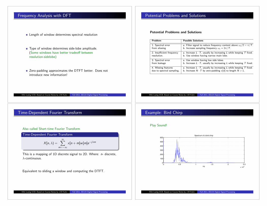
Frequency Analysis with DFT

Length of window determines spectral resolution

Type of window determines side-lobe amplitude.(Some windows have better tradeo↵ betweenresolution-sidelobe)

Zero-padding approximates the DTFT better. Does notintroduce new information!


Potential Problems and Solutions

Potential Problems and Solutions

Problem Possible Solutions

1. Spectral error a. Filter signal to reduce frequency content above !s

/2 = ⇡/T .

from aliasing b. Increase sampling frequency !s

= 2⇡/T .

2. Insu�cient frequency a. Increase L · T , usually by increasing L while keeping T fixed.

resolution. b. Use window having narrow main lobe.

3. Spectral error a. Use window having low side lobes.

from leakage b. Increase L · T , usually by increasing L while keeping T fixed.

4. Missing features a. Increase L · T , usually by increasing L while keeping T fixed.

due to spectral sampling. b. Increase N · T by zero-padding v [n] to length N > L.


Time-Dependent Fourier Transform

Also called Short-time Fourier Transform

Time-Dependent Fourier Transform

X [n,�) =1X

m=�1x [n +m]w [m]e�j�m

This is a mapping of 1D discrete signal to 2D. Where: n- discrete,�-continuous.

Equivalent to sliding a window and computing the DTFT.


Example: Bird Chirp

Play Sound!

0 0.5 1 1.5 2 2.5

x 104

0

100

200

300

400

500

600

Hz

Spectrum of a bird chirp

No temporal information!


Example: Bird Chirp

Play Sound!

0 0.5 1 1.5 2 2.5

x 104

0

100

200

300

400

500

600

Hz

Spectrum of a bird chirp

No temporal information!


Example: Bird Chirp

Instead, use Time-Dependent Fourier Transform. Plot as aspectrogram.

Time, s

Fre

qu

en

cy,

Hz

0.5 1 1.5 2 2.5 30

0.5

1

1.5

2

x 104

Trade-o↵ between temporal and spectral resolution.


Example: Bird Chirp

Instead, use Time-Dependent Fourier Transform. Plot as aspectrogram.

Time, s

Fre

qu

en

cy,

Hz

0.5 1 1.5 2 2.5 30

0.5

1

1.5

2

x 104

Trade-o↵ between temporal and spectral resolution.


Sampling the Time-Dependent Fourier Transform using

DFT

Sampling the TD-DTFT

X

r

[k] =L�1X

m=0

x [rR +m]w [m]e�j(2⇡N)km

L - is the window lengthR - jumps of samples in timeN - number of DFT samples


Miki Lustig UCB. Based on Course Notes by J.M Kahn Fall 2011, EE123 Digital Signal Processing Miki Lustig UCB. Based on Course Notes by J.M Kahn Fall 2011, EE123 Digital Signal Processing

Miki Lustig UCB. Based on Course Notes by J.M Kahn Fall 2011, EE123 Digital Signal Processing Miki Lustig UCB. Based on Course Notes by J.M Kahn Fall 2011, EE123 Digital Signal Processing

spectral analysis with the dft - university of california ...ee123/fa12/notes/lecture07.pdf · key...

Documents