spect/ct instrumentation and clinical applications spect/ct

1

William Erwin, M.S.The University of Texas

M. D. Anderson Cancer CenterHouston, TX

William Erwin, M.S.William Erwin, M.S.The University of TexasThe University of Texas

M. D. Anderson Cancer CenterM. D. Anderson Cancer CenterHouston, TXHouston, TX

SPECT/CT Instrumentation SPECT/CT Instrumentation and Clinical Applicationsand Clinical Applications


Educational Objectives:

1. Understand the underlying physical principles of SPECT/CT image acquisition, processing and reconstruction

2. Understand current and future clinical applications of SPECT/CT imaging

3. Familiarization with commercially-available SPECT/CT systems

Educational Objectives:

1. Understand the underlying physical principles of SPECT/CT image acquisition, processing and reconstruction

2. Understand current and future clinical applications of SPECT/CT imaging

3. Familiarization with commercially-available SPECT/CT systems

2


•• Brief review of SPECT principlesBrief review of SPECT principles

•• Iterative SPECT reconstructionIterative SPECT reconstruction

•• Advent of SPECTAdvent of SPECT--CT hybrid imagingCT hybrid imaging

•• Current clinical applications of SPECTCurrent clinical applications of SPECT

•• 99m99mTcTc TT1/21/2 = 6 hr, = 6 hr, γγ = 140 = 140 keVkeV

•• 111111InIn TT1/21/2 = 67 hr; = 67 hr; γγ’’s = 172, 245 s = 172, 245 keVkeV

•• 123123II TT1/21/2 = 13 hr, = 13 hr, γγ = 159 = 159 keVkeV

•• 6767GaGa TT1/21/2 = 78 hr; = 78 hr; γγ’’s = 93, 184, 296 s = 93, 184, 296 keVkeV

•• 201201TlTl TT1/21/2 = 73 hr, 70 = 73 hr, 70 keVkeV XX--rays, rays, γγ = 167 = 167 keVkeV

•• 131131II TT1/21/2 = 193 hr, = 193 hr, γγ = 364 = 364 keVkeV**

•• 153153SmSm TT1/21/2 = 46 hr, = 46 hr, γγ = 103 = 103 keVkeV**

* employed for internal therapy (* employed for internal therapy (ββ--) as well!!!) as well!!!

SPECT SPECT RadionuclidesRadionuclides

3

SPECT Imaging: Inherently 3SPECT Imaging: Inherently 3--DDAcquisition: 2Acquisition: 2--D projections of a 3D projections of a 3--D volumeD volume

Reconstruction: Reconstruction: contiguouscontiguous stack of 2stack of 2--D slicesD slices

Radon transform angular symmetry violatedRadon transform angular symmetry violated

P(θ) ≠ P(θ+π) horizontally flipped Posterior0° TDC Anterior View

SPECT ImagingSPECT Imaging

4

SPECT ImagingSPECT ImagingViolates Radon transform symmetry principle:Violates Radon transform symmetry principle:

Differential AttenuationDifferential Attenuation

b

I0

bI(θi) = I0 e-a∫ μ(L)dL

cI(θi+π) = I0 e-a∫ μ(L)dL

L

θi

I(θi)

I(θi+π)

ac

Other FactorsOther Factors•• differential, sourcedifferential, source--toto--detector distancedetector distance--dependent resolutiondependent resolution•• depthdepth--dependent scatterdependent scatter

Projections Projections over 360over 360°°instead of instead of

180180°°(exc. cardiac)(exc. cardiac)

00°°

360360°°--ΔθΔθ

θ 0°


5


Cardiac Cardiac SPECT: SPECT:

projections projections over 180over 180°°

θθ11

θθ11+180+180°°--ΔθΔθ

θθ11

00°°

Isotropic Pixels and Isotropic Pixels and VoxelsVoxels

zz

ΔΔzz = = ΔΔrr

22--D ProjectionD Projection Reconstructed SliceReconstructed Sliceyy

xx

ΔΔzz = = ΔΔyy = = ΔΔxx

rr


6


22--D Butterworth Filter (0.6 Nyquist, 10D Butterworth Filter (0.6 Nyquist, 10thth order)order)

Isotropic Isotropic Volume SmoothingVolume Smoothing↓↓ noise amplified by inverse Radon transform ramp filternoise amplified by inverse Radon transform ramp filter

22--D filtering of projections D filtering of projections ≡≡ 33--D postD post--recon filteringrecon filteringoriginaloriginal

No volume No volume smoothingsmoothing

Butterworth Butterworth 0.6 Nyquist, 0.6 Nyquist, 1010thth orderorder

7

θi

L(x,y,θi)

I0(x,y)

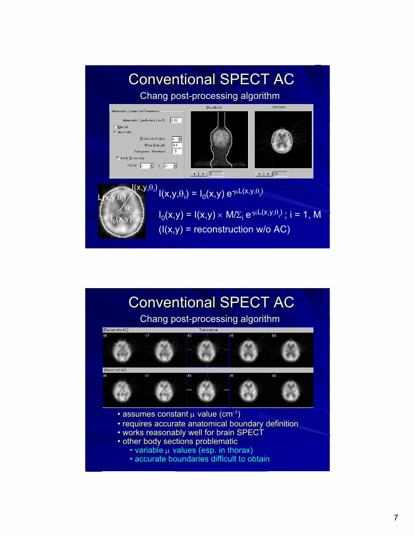
I(x,y,θi) I(x,y,θi) = I0(x,y) e-μL(x,y,θi)

I0(x,y) = I(x,y) × M/Σi e-μL(x,y,θi) ; i = 1, M(I(x,y) = reconstruction w/o AC)

Conventional SPECT ACConventional SPECT ACChang postChang post--processing algorithmprocessing algorithm

•• assumes constant assumes constant μμ value (cmvalue (cm--11))•• requires accurate anatomical boundary definitionrequires accurate anatomical boundary definition•• works reasonably well for brain SPECTworks reasonably well for brain SPECT•• other body sections problematicother body sections problematic

•• variable variable μμ values (esp. in thorax)values (esp. in thorax)•• accurate boundaries difficult to obtainaccurate boundaries difficult to obtain

Conventional SPECT ACConventional SPECT ACChang postChang post--processing algorithmprocessing algorithm

8

• Based on ideal Radon inversion formula, which:Based on ideal Radon inversion formula, which:•• assumes linear, shiftassumes linear, shift--invariant systeminvariant system•• assumes angular symmetry of projections:assumes angular symmetry of projections:

p(r,p(r,θθ) = p() = p(--r,r,θθ++ππ))•• SPECT imaging system is NOT angularly symmetric SPECT imaging system is NOT angularly symmetric nor shiftnor shift--invariant, with depthinvariant, with depth--dependent:dependent:

•• spatial resolutionspatial resolution•• attenuationattenuation•• scatterscatter(spatial and energy resolution both play a role)(spatial and energy resolution both play a role)

Conventional SPECTConventional SPECTFiltered Filtered BackprojectionBackprojection (FBP) Reconstruction(FBP) Reconstruction

• Backprojection smears information along the entire line of projection (ramp × window filter)

• Doesn’t handle source depth and scatter from it• (projections sometimes scatter corrected as a crude

“guesstimate”)• Doesn’t handle variable attenuation (μ(x,y))

• (sometimes approx. w/ constant μ and, e.g., Chang)• Doesn’t handle depth-dependent resolution

• (frequency-distance principle has been attempted)

Conventional SPECTConventional SPECTFBP ReconstructionFBP Reconstruction

9

p(r,θ)

Conventional SPECTConventional SPECTFBP Reconstruction ModelFBP Reconstruction Model

p(r,θ) = Σf(x,y)along an in-plane line integral f(x,y)

x

y

θ

SPECT ImagingSPECT Imaging•• The intensity in a voxel The intensity in a voxel b (b (n(bn(b)))), is Poisson:, is Poisson:

•• as is that in detector as is that in detector d (d (y(dy(d))))::

•• The probability that a photon emitted from voxel The probability that a photon emitted from voxel bb is detected by detector is detected by detector dd is is p(b,d)p(b,d)

( ) ( )( ( )) ( | ( ))!

nb bP n b P n b e

nλ λλ −= =

( ) ( )( ( )) ( | ( ))!

yd dP y d P y d e

yλ λλ −= =

10

SPECT ImagingSPECT ImagingTrue detector intensity = sum of true True detector intensity = sum of true voxelvoxelintensities weighted by detection probabilitiesintensities weighted by detection probabilities

Let Let x(b,d)x(b,d) = # of emissions from = # of emissions from bb measured in measured in ddMany possible sets Many possible sets x(b,d)x(b,d) →→ the measured the measured y(dy(d))x(b,d)x(b,d) is Poisson with intensityis Poisson with intensity

∑=

=B

bdbpbd

1),()()( λλ

),()(),( dbpbdb λλ =


voxel b,λb

detector d,λd

p(b,d)

11

SPECT ImagingSPECT ImagingIterative ReconstructionIterative Reconstruction

• Reconstruction based upon the Poisson statistical nature of SPECT imaging (measurement of radioactive decay)

• Can incorporate modeling of the physics of SPECT imaging• System (intrinsic + collimator) spatial resolution• Attenuation by the patient• Compton Scatter (in patient, collimator, crystal)• Collimator septal penetration• Energy resolution (future)

SPECT ImagingSPECT ImagingIterative Reconstruction MethodsIterative Reconstruction Methods

• ART (algebraic reconstruction technique)• MART (multiplicative ART)• WLS-CG (weighted least-squares conjugate gradient)

• EM (expectation maximization)!!!• ML (maximum likelihood)• MAP (maximum a posteriori)

• OS (ordered subset)!!!

12

SPECT ImagingSPECT ImagingOSOS--EM ReconstructionEM Reconstruction

•• >> >> ↑↑ rate of convergence using an ordered rate of convergence using an ordered subset of all projections at a timesubset of all projections at a time

•• A series of A series of ““minimini--EMsEMs”” performed until all performed until all projections have been cycled through per projections have been cycled through per iterationiteration

•• m OSm OS--EM iterations with n subsets EM iterations with n subsets ≅≅ m m ×× n n MLML--EM iterationsEM iterations

•• OSOS--EM parameters specified:EM parameters specified:•• # of subsets (n) and # of iterations (m)# of subsets (n) and # of iterations (m)

Expectation MaximizationExpectation Maximization

•• Estimates parameters of the statistical Estimates parameters of the statistical distributions underlying the measured data distributions underlying the measured data

•• In the case of SPECTIn the case of SPECT•• λλ of the Poisson distribution for each voxelof the Poisson distribution for each voxel•• given the measured projection datagiven the measured projection data

•• λλ represents the true count rate in each voxelrepresents the true count rate in each voxel

13

Conditional ExpectationConditional Expectation

[ 1] [ ] [ ]

[ ][ 1]

[ ]' 1

[ ][ 1]

[ ]' 1

( , ) [ ( , ) | , ] [ ( , ) | ( ), ]( ) ( , )( , )

( ', )

( ) ( ) ( , )( , )( ') ( ', )

k k k

kk

B kb

kk

B kb

x b d E x b d y E x b d y dy d b dx b d

b d

y d b p b dx b db p b d

λ λ

λλ

λλ

+

+

=

+

=

= =

=

=

∑

∑

kk+1+1thth estimate of estimate of x(b,d)x(b,d)

Maximum LikelihoodMaximum Likelihood

•• Find the parameter Find the parameter λλ that makes the that makes the measured outcome most likely.measured outcome most likely.

•• The maximum likelihood estimator of The maximum likelihood estimator of λλ is the is the measured quantity measured quantity xx..

!)|(max

xexp

x λ

λ

λλ−

=

14

1,...,

( )

( , )1,...,

1,...,

1,..., 1,..., 1,...,

( , )( ) ( | )

( )!

( ) ln ( ) ( ) ( , ) ( ) ln ( ) ( , ) ln ( , )!

To maximize with respect to (b),

0(

b B

y d

b db B

xd D

y yd D b B b B

b dl f y e

y d

L l b p b d y d b p b d x b d

b

λ λλ λ

λ λ λ λ

λ

λ

=

−=

=

= = =

∑= =

⎡ ⎤⎛ ⎞= = − + −⎢ ⎥⎜ ⎟

⎝ ⎠⎣ ⎦

∂=

∂

∑∏

∑ ∑ ∑

1,..., 1,...,' 1,...,

1,..., 1,...,' 1,...,

[ 1]

[ 1] 1

1

( ) ( , )( ) ( , )) ( ') ( ', )

( ) ( , )( ) ( , )( ', )

( , )( )

( , )

yd D d D

b B

d D d Db B

Dk

k dD

d

y d p b dL p b db p b d

y d b db p b db d

x b db

p b d

λλ

λλλ

λ

= ==

= ==

+

+ =

=

→ − +

=

=

∑ ∑ ∑

∑ ∑ ∑

∑

∑

Maximum (Log) LikelihoodMaximum (Log) Likelihood

MLML--EMEMChoose an initial parameter

λ[0]. Set k=0.

EM-step: Estimate unobserved data using λ[k] and the measurements y(d).

ML-step: Compute maximum likelihood estimate of parameter λ[k]

using estimated data.

k=k+1. Converged?

Done

1st estimate = uniform cylinder or FBP

Estimate the number of counts in each pixel of the projections that came from each voxel of the volume.

∑=+

'

][

][]1[

),'(),()(),(

b

k

kk

dbdbdydbx

λλ

Choose the next estimate of λso that it makes the estimated data above most likely.

[ 1]

[ 1] 1

1

( , )( )

( , )

Dk

k dD

d

x b db

p b dλ

+

+ =

=

=∑

∑

λ[k](b,d) = λ[k](b) p(b,d)

15

MLML--EM: One IterationEM: One Iteration

[ ][ ]

1[ 1] ' 1

1

( ) ( , )( )( ') ( ', )

( )( , )

Dk

B kdk b

D

d

y d p b dbb p b d

bp b d

λλ

λ=+ =

=

=∑

∑∑

The Key to MLThe Key to ML--EMEM

•• The probability (or system) matrix inThe probability (or system) matrix in

•• p(b,d)p(b,d) captures the probability that a count in captures the probability that a count in a particular voxel of the volume will wind up a particular voxel of the volume will wind up in a particular pixel in a particular projection.in a particular pixel in a particular projection.

[ 1]

[ 1] 1

1

( , )( )

( , )

Dk

k dD

d

x b db

p b dλ

+

+ =

=

=∑

∑

16

p(b,dp(b,d) Can Capture:) Can Capture:

1. Depth1. Depth--dependent resolutiondependent resolution2. Position2. Position--dependent scatter in the patientdependent scatter in the patient3. Depth3. Depth--dependent attenuationdependent attenuation

We can thus use a measured attenuation map We can thus use a measured attenuation map along with models of scatter and camera along with models of scatter and camera resolution to perform a far more accurate resolution to perform a far more accurate reconstruction.reconstruction.

Warning, though: GIGO principle applies!!!Warning, though: GIGO principle applies!!!

SPECT MLSPECT ML--EM Flow DiagramEM Flow Diagram

Fest = recon est.PDM = p(b,d)Pest = proj. est.P = measured proj.errest = proj. est. errorr = damping factor (0<r≤1)

Note: In practice (i.e., in the clinic), the stopping criteria is number of iterations (time constraint) instead of a convergence criteria.

P ÷ Pest

×

17

1.1. PrePre--filtering of original projectionsfiltering of original projections

2.2. Regularization: Maximum ARegularization: Maximum A--Priori Priori (MAP) EM algorithms(MAP) EM algorithms•• prior knowledge (e.g., anatomical)prior knowledge (e.g., anatomical)•• smoothness criteriasmoothness criteria

3.3. PostPost--filtering of reconstructed volume, filtering of reconstructed volume, e.g., Gaussian (filter FWHM specified)e.g., Gaussian (filter FWHM specified)

SPECT Iterative ReconstructionSPECT Iterative ReconstructionNoise Reduction (Smoothing)Noise Reduction (Smoothing)

Median Root Prior (MRP) PenalizedMedian Root Prior (MRP) Penalized--LikelihoodLikelihood

M(bM(b)) obtained from median filter of image of obtained from median filter of image of λλ[k][k](b(b))

ββ = unit= unit--less control parameterless control parameter

SPECT Iterative ReconstructionSPECT Iterative ReconstructionMAPMAP--EM ExampleEM Example

[ ][ ]

[ ]1' 1

[ 1]

1

( ) ( , )( )( ) ( )( ') ( ', ) [ ]

( )( )( , )

Dk

kB kdb

kD

d

y d p b dbb M bb p b dM bb

p b d

λλλ β

λ

==

+

=

−+

=

∑∑

∑

18

p(r,θ) = Σf(x,y)×pattn(x,y,r,θ)along a line integral

pattn(x,y,r,θ) = probability due to attenuation

pattn(x,y,r,θ) = exp(-Σabμ(x’,y’)Δ(x’,y’))

p(r,θ)

f(x,y)

x

y

θ

SPECT Iterative ReconstructionSPECT Iterative ReconstructionAttenuation ModelingAttenuation Modeling

a

b


CTCT--Based Based Attenuation Attenuation

MapMap(μ(μ map)map)

Can account for Can account for variably attenuating variably attenuating

mediamedia

19


99m99mTc Tc SestaMIBISestaMIBI

(Parathyroid (Parathyroid adenoma)adenoma)

w/ AMw/ AM w/o AMw/o AM

SPECT Iterative ReconstructionSPECT Iterative ReconstructionSystem Resolution (System Resolution (RRss) Modeling) Modeling

DistanceDistance--dependent collimator beam dependent collimator beam

________________RRss = = √√ RRii

22 + R+ Rcc22

Pencil Beam (FBP)

Fan Beam (2D iterative)-

Cone Beam (3D iterative)

IntrinsicDetector

ResolutionRi

r Collimator ResolutionRc a linear function vs r

20

p(r,θ)

f(x,y)

x

y

θ

SPECT Iterative ReconstructionSPECT Iterative ReconstructionSystem Resolution ModelingSystem Resolution Modeling

2D: p(r,θ) = Σf(x,y)×pres(x,y,r,θ)3D: p(r,θ) = Σf(x,y,z)×pres(x,y,z,r,θ)pres = probability due to resolution

“fan of acceptance” (2D fan beam model)“cone of acceptance” (3D cone beam model)


CollimatorCollimator--Detector Response Function (CDRF) Detector Response Function (CDRF)

Intrinsic Response (IRF)Intrinsic Response (IRF)++

Geometric Response (GRF)Geometric Response (GRF)

SeptalSeptal Penetration Response (SPRF)Penetration Response (SPRF)

SeptalSeptal Scatter Response (SSRF)Scatter Response (SSRF)

21


CollimatorCollimator--Detector Response Function (CDRF) Detector Response Function (CDRF)

Depends upon:Depends upon:

•• Radionuclide Gamma Emissions/Energies, e.g.,Radionuclide Gamma Emissions/Energies, e.g.,•• TcTc--99m (140 99m (140 keVkeV))•• II--131 (364 131 (364 keVkeV + 637, 723 + 637, 723 keVkeV))

•• Energy Energy Window(sWindow(s), e.g.,), e.g.,•• II--131 (364 keV/15%)131 (364 keV/15%)•• InIn--111 (174 keV/15%, 245/15%)111 (174 keV/15%, 245/15%)

•• Collimator ParametersCollimator Parameters•• hole shape/diameter/length (geometric response)hole shape/diameter/length (geometric response)•• septalseptal thickness (thickness (septalseptal penetration/penetration/septalseptal scatter)scatter)


Standard Standard Filtered Filtered

BackprojectionBackprojection

22--D OSEMD OSEMw/ fan beam w/ fan beam

modeling modeling (m=12,n=10)(m=12,n=10)

99m99mTc Bone Scan, LowTc Bone Scan, Low--Energy HighEnergy High--Resolution CollimatorResolution Collimator

22--D preD pre--filter: Butterworth, filter: Butterworth, fcfc = 0.6 Nyquist, order = 10= 0.6 Nyquist, order = 10

33--D Gaussian PostD Gaussian Post--Filter (7.8 mm FWHM)Filter (7.8 mm FWHM)

33--D OSEMD OSEMw/ cone beam w/ cone beam


22


6767Ga Citrate, MediumGa Citrate, Medium--Energy LowEnergy Low--Penetration CollimatorPenetration Collimator

33--D Gaussian PostD Gaussian Post--Filter (9.6 mm FWHM)Filter (9.6 mm FWHM)

22--D preD pre--filter: Butterworth, filter: Butterworth, fcfc = 0.65 Nyquist, order = 7= 0.65 Nyquist, order = 7

FBPFBP

22--D OSEMD OSEMw/ fan beam w/ fan beam


33--D OSEMD OSEMw/ cone w/ cone beam beam


p(r,θ)

f(x,y)

x

y

θ

SPECT Iterative ReconstructionSPECT Iterative ReconstructionAttenuation and Resolution ModelingAttenuation and Resolution Modeling

2D: p(r,θ) = Σf(x,y)×pres(x,y,r,θ)×pattn(x,y,r,θ) 3D: p(r,θ) = Σf(x,y,z)×pres(x,y,z,r,θ)×pattn(x,y,z,r,θ)

23

•• Reduces contrastReduces contrast•• low frequency blur to the imagelow frequency blur to the image

•• Depends onDepends on•• photon energyphoton energy•• camera energy resolution, window settingcamera energy resolution, window setting•• object shapes, object shapes, ρρ‘‘s, radionuclide distributionss, radionuclide distributions

•• Compensation must occur before attenuationCompensation must occur before attenuation•• attenuation assumes complete removal of attenuation assumes complete removal of

attenuated photons from the attenuated photons from the ““beambeam““•• in SPECT imaging, in SPECT imaging, ““beambeam““ contains scattercontains scatter

SPECT Imaging: Compton ScatterSPECT Imaging: Compton Scatter

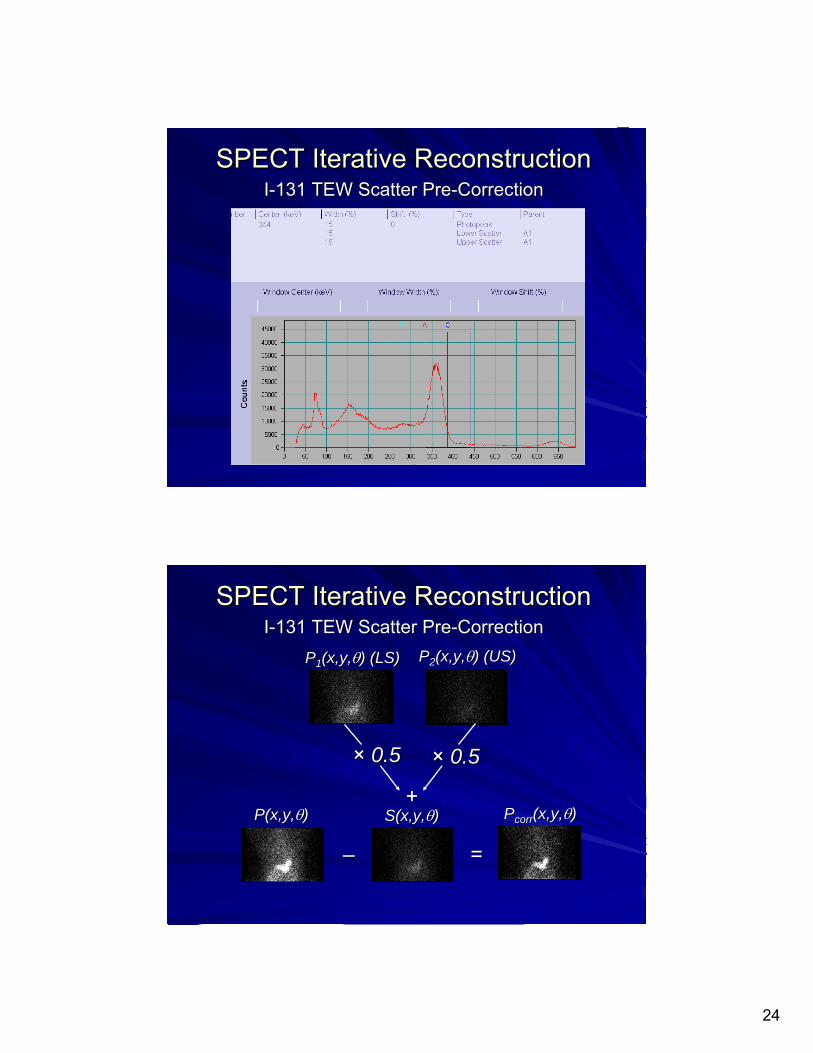
•• For each For each photopeakphotopeak projection image, projection image, P(x,y,P(x,y,θθ)), , estimate scatter as a weighted sum of one (dualestimate scatter as a weighted sum of one (dual--energyenergy--window) or two (triplewindow) or two (triple--energyenergy--window) window) adjacent scatter window images, adjacent scatter window images, CCii(x,y,(x,y,θθ))..

•• Subtract scatter prior to reconstruction:Subtract scatter prior to reconstruction:

S(x,y,S(x,y,θθ) = ) = ΣΣii kkii ×× CCii(x,y,(x,y,θθ))

PPcorrcorr(x,y,(x,y,θθ)) →→ P(x,y,P(x,y,θθ)) –– S(x,y,S(x,y,θθ))

kkii = scatter window image i weighting factor= scatter window image i weighting factor

SPECT Iterative ReconstructionSPECT Iterative ReconstructionDEW/TEW Scatter PreDEW/TEW Scatter Pre--CorrectionCorrection

24

SPECT Iterative ReconstructionSPECT Iterative ReconstructionII--131 TEW Scatter Pre131 TEW Scatter Pre--CorrectionCorrection

SPECT Iterative ReconstructionSPECT Iterative ReconstructionII--131 TEW Scatter Pre131 TEW Scatter Pre--CorrectionCorrection

×× 0.50.5 ×× 0.50.5

++

––

P(x,y,P(x,y,θθ))

==

PP11(x,y,(x,y,θθ) (LS)) (LS) PP22(x,y,(x,y,θθ) (US)) (US)

S(x,y,S(x,y,θθ)) PPcorrcorr(x,y,(x,y,θθ))

25

•• Estimate scatter contribution to each Estimate scatter contribution to each photopeak projection pixel d, photopeak projection pixel d, S(dS(d)), as a , as a weighted sum of counts, weighted sum of counts, CCii(d(d)), from one , from one (DEW) or two (TEW) adjacent scatter (DEW) or two (TEW) adjacent scatter windowswindows

•• Incorporate into the forward projection step:Incorporate into the forward projection step:

PP''estest(d(d)) →→ PPestest(d(d)) + + S(dS(d))

S(dS(d) = ) = ΣΣii kkii ×× CCii(d(d))

SPECT Iterative ReconstructionSPECT Iterative ReconstructionDEW/TEW Iterative Scatter ModelingDEW/TEW Iterative Scatter Modeling


×× 0.50.5 ×× 0.50.5

++

PP11(d) (LS)(d) (LS) PP22(d) (US)(d) (US)

S(dS(d))

26


scatter contribution to detector scatter contribution to detector y(d)y(d) incorporated into forward projectorincorporated into forward projector

[ ][ ]

1[ 1] ' 1

1

( ) ( , )( )[ ( ') ( ', ) ( )]

( )( , )

Dk

B kdk b

D

d

y d p b dbb p b d S d

bp b d

λλ

λ=+ =

=

+=

∑∑

∑

CurrentRecon

Estimate⊗ Scatter

Kernel ×

ρ Map

ESS

ForwardProject

w/ Attenuation

μ Map

Next ProjectionScatter Estimate

S(d)

Effective Scatter Source EstimationEffective Scatter Source Estimation

27

SPECT Iterative ReconstructionSPECT Iterative ReconstructionScatter Modeling in the System Matrix Scatter Modeling in the System Matrix p(b,dp(b,d))

d

b

p(b,d) = pS(b)×pS(b,d)×pA(b,d)×pD×pE

pS(b) = prob. of scatterpS(b,d) = prob. of scatter into det. dpA(b,d) = prob. due to attenuationpD = prob. due to det. efficiencypE = prob. due to energy resolution

•• SPECT Attenuation CorrectionSPECT Attenuation Correction•• Quantitative SPECT Quantitative SPECT ≡≡ NMNM’’s s ““holy grailholy grail””

•• requires attenuation artifact removal forrequires attenuation artifact removal for•• absolute quantification of uptake in 3absolute quantification of uptake in 3--D (like PET)D (like PET)(accurate scatter correction also needed)(accurate scatter correction also needed)

•• Previous AC methods have not worked wellPrevious AC methods have not worked well•• constant constant μμ prepre--/post/post--processing (e.g., Sorenson, Chang)processing (e.g., Sorenson, Chang)•• radioactive sourceradioactive source--based transmission CT attachmentsbased transmission CT attachments

•• Improved LocalizationImproved Localization•• FunctionalFunctional--anatomical overlay (image fusion)anatomical overlay (image fusion)

•• requires registered dualrequires registered dual--modality datamodality data

(Future: CT = scatter modeling media)(Future: CT = scatter modeling media)

SPECT/CT Imaging: Why?SPECT/CT Imaging: Why?

28

SPECT/CT Image RegistrationSPECT/CT Image Registration

Methods:- Manual

w/o or w/ fiducials- Semi-automated

- fiducials- anat. landmarks

- Automated- AIR- Mutual Info.

SPECT/CT Imaging: SoftwareSPECT/CT Imaging: Software

Registered CT ImageRegistered CT Image--Based SPECT Based SPECT μμ MapMap

Parameters:- HU-to-cm-1 function

- piece-wise bilinear (most common)

Effective keV- CT (~ 70 – 80)- SPECT (nuclide dep.)

- Attenuation beam model- narrow- broad(w/o scatter correction)

- μ map image smoothing

But what if CT and SPECT beds are not identical? UhBut what if CT and SPECT beds are not identical? Uh--oh! GIGO!oh! GIGO!


29

0

0.1

0.2

0.3

0 100 200 300 400 500

Energy (keV)

μ/ρ(cm/g)

Air Muscle Bone

CT

Material attenuation versus EnergyMaterial attenuation versus EnergyCT-Based SPECT μ ValuesCTCT--Based SPECT Based SPECT μμ ValuesValues

keVCT: 75 (effective)SPECT: 140 (99mTc)

Transform[HU+1000]×μ75(H2O)

μ140(m) = ----------------------------1000×[μ75(m)/μ140(m)]μ75(H2O)0.188 cm-1

material m [μ75(m)/μ140(m)]1.22 (HU ≤ 0)1.43 (HU > 0)

Example CT HUExample CT HU--toto--SPECT cmSPECT cm--11 transformtransform(standard: piece(standard: piece--wise bilinear function)wise bilinear function)

CT Number-to-Tc-99m μ value Function

0

0.05

0.1

0.15

0.2

0.25

0.3

-100

0 0

1000

CT Number (HU)

μ v

alue

(cm

-1)

CT-Based SPECT μ ValuesCTCT--Based SPECT Based SPECT μμ ValuesValues

Air/water mixture

water/bone mixture

30

Iterative ReconstructionIterative Reconstruction

FBP w/FBP w/Butterworth 0.4/5Butterworth 0.4/5

99m99mTc ECTc EC--DG (NSCLC)DG (NSCLC)

33--D OSEM w/ D OSEM w/ resolution modelingresolution modeling

33--D OSEM w/ D OSEM w/ resolution and resolution and

attenuation attenuation modelingmodeling


Original Original ““SPECT/CTSPECT/CT”” scannersscannersGdGd--153 (100 153 (100 keVkeV γγ) source ) source ““transmission CTtransmission CT””

Scanning Lines Stationary Lines LimitationsLimitations

1.1. Poor resolution/partial Poor resolution/partial volume (esp. air, lung, soft volume (esp. air, lung, soft tissue, bone interfaces)tissue, bone interfaces)

2.2. Poor statistics (noisy Poor statistics (noisy images, heavy smoothing)images, heavy smoothing)

3.3. DeadDead--time (imaged with time (imaged with gamma camera detector)gamma camera detector)

4.4. Emission Contamination Emission Contamination (e.g., Tc(e.g., Tc--99m 99m downscatterdownscatter))

5.5. Designed for cardiacDesigned for cardiac

Supplanted by SPECT/XSupplanted by SPECT/X--ray CTray CT

31

HawkeyeHawkeye®®(Original 1(Original 1--slice CT)slice CT)

InfiniaInfinia / / VCVC HawkeyeHawkeye--4 4 (Current 4(Current 4--slice CT)slice CT)

Slide courtesy of Slide courtesy of OsnatOsnat Zak, GE HealthcareZak, GE Healthcare

SPECT/CT Imaging: HardwareSPECT/CT Imaging: HardwareHawkeyeHawkeye®® (GE Healthcare)(GE Healthcare)

SPECT/CT Imaging: HardwareSPECT/CT Imaging: Hardware

Slide Courtesy of Slide Courtesy of OsnatOsnat Zak, GE HealthcareZak, GE Healthcare

32

• mA: 1.0 – 2.5• kVp: 140 (default), 120• Collimation: 4 × 5 mm• Slice Thickness: 5 mm (axial)• Acq. Time (axial): 15 sec/20 mm (180º + fan)

or 5 min/40 cm• FOV: 45 cm (512 × 512 = 0.88 × 0.88 pixels)• Patient Port: 60 cm

SPECT/CT Imaging: HardwareSPECT/CT Imaging: HardwareHawkeyeHawkeye--4 CT (GE Healthcare)4 CT (GE Healthcare)

Dose Comparison (40 cm)

>6.5 mSv1.8 mSv0.72 mSvPatient Patient dosedose

20-80 mA2.5mA1mATube Tube currentcurrent

120-140 kVp140 kVp140 kVpXX--ray tube ray tube voltagevoltage

Conventional CTHawkeye4Hawkeye4

Design Considerations• Low radiation dose• Time Averaged CT• Accurate SPECT-CT alignment • Integration & Workflow• Same gantry and footprint


SPECT/CT Imaging: HardwareSPECT/CT Imaging: Hardware


20 min 10 minGE HawkeyeBone WB 40cm CT AC + Anatomy

15 min 45 Minutesx 1 SPECT View

Bone WB

10 min 5 minGE Hawkeye-4Evolution for Bone 15 min 30 Minutes

x 1 SPECT Views

10 min30 min

80 cm CT AC + Anatomy x 3 SPECT Views

40 MinutesGE Hawkeye-4Evolution for Bone

40cm CT AC + Anatomy

EvolutionIterative Recon

includesCollimator-Detector

Response

33

SPECT/CT Imaging: HardwareSPECT/CT Imaging: HardwarePhilips HealthcarePhilips Healthcare

Precedence 6 & 16 BrightView XCT(New)

Slide Courtesy of Ling Slide Courtesy of Ling ShaoShao, Philips Healthcare, Philips Healthcare

SPECT/CT Imaging: HardwareSPECT/CT Imaging: HardwarePrecedence (Philips Healthcare)Precedence (Philips Healthcare)

•• kVpkVp: 90, 120 or 140: 90, 120 or 140•• mAmA: 20 : 20 –– 500500•• FOV: 50 cm (512 FOV: 50 cm (512 ×× 512 = 0.98 512 = 0.98 ×× 0.98 pixels) up to 150 cm (axial)0.98 pixels) up to 150 cm (axial)•• Collimation:Collimation:

•• 66--slice: 2 slice: 2 ×× 0.6, 6 0.6, 6 ×× 0.75, 6 0.75, 6 ×× 1.5, 6 1.5, 6 ×× 3, 4 3, 4 ×× 4.5, 4 4.5, 4 ×× 6.0 mm6.0 mm•• 1616--slice: 2 slice: 2 ×× 0.6, 16 0.6, 16 ×× 0.75, 16 0.75, 16 ×× 1.5, 8 1.5, 8 ×× 3, 4 3, 4 ×× 4.5 mm4.5 mm

Slice Thickness: 0.65 Slice Thickness: 0.65 -- 7.5 mm (spiral), 0.6 7.5 mm (spiral), 0.6 -- 12 mm (axial)12 mm (axial)Scan Speed (spiral)Scan Speed (spiral)

•• 0.4, 0.5, 0.75, 1, 1.5, 2 sec/3600.4, 0.5, 0.75, 1, 1.5, 2 sec/360°°; 0.28, 0.33 sec/240; 0.28, 0.33 sec/240°°•• Patient Port: 70 cmPatient Port: 70 cm•• Resolution: 24 Resolution: 24 lplp/cm/cm•• Dose (CTDI): 12.85 mGy/100 Dose (CTDI): 12.85 mGy/100 mAsmAs (head), 6.5 mGy/100 (head), 6.5 mGy/100 mAsmAs (body)(body)•• Registration error Registration error ≤≤ 4mm (one pixel)4mm (one pixel)


34

SPECT/CT Imaging: HardwareSPECT/CT Imaging: HardwareBrightViewBrightView XCT (Philips Healthcare)XCT (Philips Healthcare)


•• Flat Panel Volume CT technologyFlat Panel Volume CT technology•• Coplanar with SPECT ImagingCoplanar with SPECT Imaging

(cardiac (cardiac --14 cm)14 cm)•• Localization, CTLocalization, CT--AC, Bone ImagingAC, Bone Imaging•• Max. Rotation SpeedMax. Rotation Speed

12 sec for 36012 sec for 360ºº (14 cm axial FOV)(14 cm axial FOV)Slice thicknessSlice thickness

0.33 0.33 –– 2.0+ mm (isotropic 2.0+ mm (isotropic voxelvoxel))Resolution: >15 Resolution: >15 lplp/cm/cmDose (CTDI) Dose (CTDI) -- Typical:Typical:

•• ~6 ~6 mGymGy (body localization)(body localization)•• ~1 ~1 mGymGy (AC)(AC)

Registration errorRegistration error≤≤ 4mm (one pixel)4mm (one pixel)

•• Volumetric CT components Volumetric CT components •• Rotating anode XRotating anode X--ray tube ray tube •• 120 120 kVpkVp XX--ray generatorray generator

pulsed or continuouspulsed or continuous•• 4030CB flat panel detector4030CB flat panel detector

10, 30, 60 fps, dynamic gain10, 30, 60 fps, dynamic gain•• XX--ray collimator and beam shaperray collimator and beam shaper•• CBCT image recons using GPUCBCT image recons using GPU

Volumetric CT system goalsVolumetric CT system goals•• XX--ray coneray cone--beam overlaps SPECT beam overlaps SPECT

FOVFOV•• 360360oo Gantry rotation within a Gantry rotation within a

breathbreath--holdhold•• LowLow--dose CT dose CT acqacq. parameters. parameters•• Integrated hybrid software solutionIntegrated hybrid software solution

35

SPECT/CT Imaging: ReconstructionSPECT/CT Imaging: ReconstructionAstonish (Philips Healthcare)Astonish (Philips Healthcare)

•• 3D Astonish OSEM Reconstruction3D Astonish OSEM Reconstruction•• Resolution, attenuation and scatter correctionsResolution, attenuation and scatter corrections•• MultipleMultiple--peak isotopepeak isotope•• > 5 mm SPECT reconstruction resolution > 5 mm SPECT reconstruction resolution

•• HalfHalf--time Acquisitiontime Acquisition•• Equal or better image quality with AstonishEqual or better image quality with Astonish

•• Typical SPECT/CT acquisitionTypical SPECT/CT acquisition•• Bone scanBone scan

15 min SPECT + 2 min CT 15 min SPECT + 2 min CT 7 min + 2 min7 min + 2 min•• Cardiac scanCardiac scan

•• 15 min SPECT + 2 min CT 15 min SPECT + 2 min CT 7 min + 2 min7 min + 2 min

FBP

Astonish


11--, 2, 2--, 6, 6-- or 16or 16--slice CTslice CT

CT

SPECT/CT Imaging: HardwareSPECT/CT Imaging: HardwareSymbiaSymbia®® T (Siemens Medical Solutions USA)T (Siemens Medical Solutions USA)

36

Scalable/Scalable/UgradeableUgradeable


S(SPECT only)

T

T2

T6

T16

___T T2 T6 T16_____

Collimation (mm) 2×1.0 to 2×5 6×0.5 to 6×3 16×0.6 to 16×1.2

Max. speed (360º) 0.8 s 0.6 s 0.5 s

Slices/rotation 2 6 16

kVp 80, 110, 130

mA* 30 – 240 20 - 345

Slice width (mm) 3, 5, 8 1 - 10 0.63 - 10 0.6 - 10

FOV (cm) 50 (512 × 512 = 0.98 × 0.98 pixels) up to 200 (axial)

Patient Port 70 cm

*CARE Dose 4D AEC+DOM dynamic dose reduction algorithm(~8 – 12 mGy CTDIvol @ 130 kVp/90 ref. mA)


37

SPECT/CT Imaging: ReconstructionSPECT/CT Imaging: ReconstructionFlash3D (Siemens Medical Solutions USA)Flash3D (Siemens Medical Solutions USA)

•• Flash3D OSEM ReconstructionFlash3D OSEM Reconstruction•• 3D collimator resolution compensation3D collimator resolution compensation

in both forward and backin both forward and back--projection directionsprojection directions3D Gaussian PSF v. distance from collimator3D Gaussian PSF v. distance from collimator

•• Attenuation compensation (CTAttenuation compensation (CT--based AC maps)based AC maps)•• Scatter compensationScatter compensation

DEW/TEWDEW/TEW--based scatter projection imagesbased scatter projection imagesAdditive in forward projectionAdditive in forward projection

•• MultipleMultiple--peak isotopespeak isotopes•• Each Each photopeakphotopeak reconstructed separatelyreconstructed separately•• AC maps and scatter images for each peakAC maps and scatter images for each peak•• PostPost--summation of peak reconstructionssummation of peak reconstructions

SPECT/CT Imaging: ReconstructionSPECT/CT Imaging: ReconstructionFlash3D (Siemens Medical Solutions USA)Flash3D (Siemens Medical Solutions USA)

FBP

Flash3D

38

μμ(material(x,y,z), (material(x,y,z), γγhighhigh) computed () computed (6767Ga Ga γγhighhigh = 296 = 296 keVkeV))

μμ((γγlowlow) = ) = μμ((γγhighhigh) ) ×× ααlowlow

ααlowlow = = μ(μ(HH22O,low) / O,low) / μ(μ(HH22O,high)O,high)

6767Ga: Ga: αα93keV93keV = 1.476, = 1.476, αα184keV184keV = 1.197= 1.197

AF=AF=ee--∫∫μμ(L(Lθθ)dL)dLθθ))AF(x,y,AF(x,y,θθ))multimultiγγ = = ΣΣ WWγγii ×× AFAFγγii ((WWγγii = = relrel. Wt. of . Wt. of γγii))

((6767Ga: WGa: W9393 = .54, W= .54, W184184 = .295, W= .295, W296296 = .165 [measured])= .165 [measured])

(Note: bone attenuation will be underestimated)(Note: bone attenuation will be underestimated)

SPECT/CT Imaging: AC MapSPECT/CT Imaging: AC MapMultiMulti--γγ Radionuclide (GE Hawkeye 1Radionuclide (GE Hawkeye 1--Slice)Slice)

172 172 keVkeV photopeakphotopeak

247 247 keVkeV photopeakphotopeak

172 172 keVkeV lower scatterlower scatter

111111InIn

172 172 keVkeV upper scatterupper scatter

247 247 keVkeV lower scatterlower scatter

SPECT/CT Imaging: AC MapSPECT/CT Imaging: AC MapMultiMulti--γγ Radionuclide (Siemens Radionuclide (Siemens SymbiaSymbia T)T)

39

111111In 172 In 172 keVkeV photopeakphotopeak 111111In 247 In 247 keVkeV photopeakphotopeak

SPECT/CT Imaging: AC MapSPECT/CT Imaging: AC MapMultiMulti--γγ Radionuclide (Siemens Radionuclide (Siemens SymbiaSymbia T)T)

SPECT/CT Imaging: HardwareSPECT/CT Imaging: HardwareNMNM--CT FOV CalibrationCT FOV Calibration

1.1. SPECT/CT = SPECT and CT scanning with a SPECT/CT = SPECT and CT scanning with a common patient handling system (bed)common patient handling system (bed)

2.2. Scanners are mechanically aligned (Scanners are mechanically aligned (±± tolerance)tolerance)3.3. Same anatomical slice must be aligned SPECTSame anatomical slice must be aligned SPECT↔↔CTCT4.4. Minor adjustment needed to correct for residual Minor adjustment needed to correct for residual

alignment errors between the two alignment errors between the two FOVsFOVs•• Transformation: Transformation: ΔΔxx, , ΔΔyy, , ΔΔzz, , ΔαΔα, , ΔβΔβ, , ΔγΔγ

5.5. Calibration for each set of collimators and detector Calibration for each set of collimators and detector configuration (180configuration (180ºº and 90and 90ºº) may be required) may be required

40

SPECT/CT Imaging: HardwareSPECT/CT Imaging: HardwareNMNM--CT FOV Calibration: GE HawkeyeCT FOV Calibration: GE Hawkeye

Alignment Phantom containing 6 landmarks (m99Tc solution in standard syringes) is scanned by both SPECT and CT

• Automatically Detects the landmarks• Calculates the offsets in X, Y, Z and θ• Applies the offsets to SPECT-CT scans


SPECT/CT Imaging: HardwareSPECT/CT Imaging: HardwareNMNM--CT FOV Calibration: Siemens CT FOV Calibration: Siemens SymbiaSymbia

• 10 point sources• Spiked with:

• CT contrast material• Tc-99m activity

SPECT-CT acquisiton/reconstruction of sources placed in plastic holders

performed

Cotton swab tip in plastic vial

41



Iteratively solve for

transformation matrix

42

SPECT/CT Imaging: HardwareSPECT/CT Imaging: HardwareExample NMExample NM--CT FOV Registration TestCT FOV Registration Test

ACR SPECT phantom

50 μCi Co-57button sources

(~10 μCi eff. in Tc-99menergy window)


43


CT μ map artifacts:CT CT μμ map artifacts:map artifacts:everything BUT contrast and motioneverything BUT contrast and motion

FOV FOV truncationtruncation

Detector Detector ProblemsProblems

Metal Object in Metal Object in PocketPocket

ZipperZipper

44

CT μ map artifactsCT CT μμ map artifactsmap artifactsCT contrast materialCT contrast material

4 hr 4 hr 111111In In OctreoOctreo μμ mapmap 24 hr 24 hr 111111In In OctreoOctreo μμ mapmap

CT μ map artifactsCT CT μμ map artifactsmap artifactsCT contrast materialCT contrast material

4 hr 4 hr 111111In OctreotideIn Octreotide 24 hr 24 hr 111111In OctreotideIn OctreotideActivity Activity created!!!created!!!

45

Contemporaneous, NOT

simultaneous, SPECT and CT

scans!!!

Thus, there can be patient motion

between the two scans!!!

adenoma

SPECT/CT: MotionSPECT/CT: MotionSPECT/CT: MotionSestaMIBI Parathyroid

SPECT/CT: Motion CorrectionSPECT/CT: Motion CorrectionSPECT/CT: Motion CorrectionSestaMIBI Parathyroid

adenoma

46

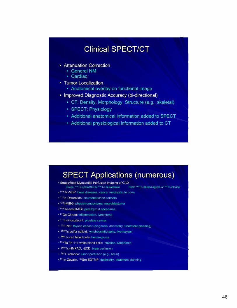
Clinical SPECT/CTClinical SPECT/CT

•• Attenuation CorrectionAttenuation Correction•• General NMGeneral NM•• CardiacCardiac

•• Tumor LocalizationTumor Localization•• Anatomical overlay on functional imageAnatomical overlay on functional image

•• Improved Diagnostic Accuracy (biImproved Diagnostic Accuracy (bi--directional)directional)•• CT: Density, Morphology, Structure (e.g., skeletal)CT: Density, Morphology, Structure (e.g., skeletal)•• SPECT: PhysiologySPECT: Physiology•• Additional anatomical information added to SPECTAdditional anatomical information added to SPECT•• Additional physiological information added to CTAdditional physiological information added to CT

•• Stress/Rest Myocardial Perfusion Imaging of CADStress/Rest Myocardial Perfusion Imaging of CADStress: Stress: 99m99mTcTc--sestaMIBI or sestaMIBI or 99m99mTcTc--TetrafosminTetrafosmin Rest: Rest: 99m99mTcTc--labeled agents or labeled agents or 201201Tl chlorideTl chloride

•• 99m99mTcTc--MDP: MDP: bone diseases, cancer metastatic to bonebone diseases, cancer metastatic to bone

• 111111InIn--Octreotide: Octreotide: neuroendocrine cancersneuroendocrine cancers

•• 123123II--MIBG: MIBG: pheochromocytomapheochromocytoma, , neuroblastomaneuroblastoma

•• 99m99mTcTc--sestaMIBI: sestaMIBI: parathyroid adenomasparathyroid adenomas

• 6767GaGa--Citrate: Citrate: inflammation, lymphomainflammation, lymphoma

•• 111111InIn--ProstaScint: ProstaScint: prostate cancerprostate cancer

•• 131131II--NaI: NaI: thyroid cancer (diagnosis, thyroid cancer (diagnosis, dosimetrydosimetry, treatment planning), treatment planning)

•• 99m99mTcTc--sulfur colloid: sulfur colloid: lymphoscintigraphylymphoscintigraphy, liver/spleen, liver/spleen

•• 99m99mTcTc--red blood cells: red blood cells: hemangiomahemangioma

•• 99m99mTcTc--/In/In--111 white blood cells: 111 white blood cells: infection, lymphomainfection, lymphoma

•• 99m99mTcTc--HMPAO, HMPAO, --ECD: ECD: brain perfusionbrain perfusion

•• 201201Tl chloride: Tl chloride: tumor perfusion (e.g., brain)tumor perfusion (e.g., brain)

•• 111111InIn--Zevalin,Zevalin, 153153SmSm--EDTMP: EDTMP: dosimetrydosimetry, treatment planning, treatment planning

SPECT Applications (numerous)SPECT Applications (numerous)

47

Images Courtesy of Tel-Aviv Sourasky Medical Center

Hawkeye-4 with Evolution for Bone Advanced Reconstruction

Tc-99m Bone Study

88 YOM, referred for a bone scintigraphydue to severe back pain. On a regular X-ray, a fracture was detected at T11, raising the differential diagnosis between an old and a recent fracture.

On SPECT-CT bone scintigraphy, increased uptake was detected at T11 including the anterior and posterior vertebral elements compatible with a recent fracture.


TcTc--99m Bone SPECT/CT (Hawkeye)99m Bone SPECT/CT (Hawkeye)

•• 202 lbs (92 kg), Male, 25 yrs, 202 lbs (92 kg), Male, 25 yrs, DxDx: Right knee sarcoma, One 24: Right knee sarcoma, One 24--s CTs CTCT parametersCT parameters:: SPECT parametersSPECT parameters::120 kVp/80 120 kVp/80 mAmA 25.3 25.3 mCimCi TcTc--99m MDP, 3 hrs 99m MDP, 3 hrs p.ip.i..10 ms pulse, 14.9 10 ms pulse, 14.9 mGymGy CTDICTDIVOLVOL 128 x 128 , 128 views, 20 s, 1.4 zoom128 x 128 , 128 views, 20 s, 1.4 zoomCT CT resamplingresampling::

0.64 mm 0.64 mm voxelsvoxels

TcTc--99m MDP Bone (99m MDP Bone (BrightViewBrightView))


Images courtesy of Radiological Associates of Sacramento

48

WB Bone SPECT/CT: CT First (Symbia)WB Bone SPECT/CT: CT First (WB Bone SPECT/CT: CT First (SymbiaSymbia))

•• Top of headTop of head--toto--mid thighmid thigh

•• 36.4 cm axial FOV per bed36.4 cm axial FOV per bed

•• CT scan length set to 109.2 cm CT scan length set to 109.2 cm (36.4 cm (36.4 cm ×× 3)3)

•• CT scan FOV adjusted axiallyCT scan FOV adjusted axially

•• Max. CT recon FOV (50 cm)Max. CT recon FOV (50 cm)

•• 2.5 mm thick/2 mm increment2.5 mm thick/2 mm increment

•• Followed by 3Followed by 3--bed SPECT over bed SPECT over same axial FOVsame axial FOV

•• NCO Continuous AcquisitionNCO Continuous Acquisition

•• 180 views x 5 sec/view180 views x 5 sec/view

•• 7.5 min total acquisition time/bed7.5 min total acquisition time/bed

•• 3 beds: 25 min3 beds: 25 min

•• 4 beds: 34 min4 beds: 34 min

•• Recon: 15 ss/8 iters 8 mm filterRecon: 15 ss/8 iters 8 mm filter

Whole Body Bone SPECT AcquisitionWhole Body Bone SPECT AcquisitionWhole Body Bone SPECT Acquisition

49

Whole Body Bone SPECT/CTWhole Body Bone SPECT/CTWhole Body Bone SPECT/CT

4-Bed Bone SPECT/CT (Symbia)44--Bed Bone SPECT/CT (Bed Bone SPECT/CT (SymbiaSymbia))

50

Parathyroid adenoma localized with SPECT/CT

1.25 mm thick/1.0 mm increment 25 cm FOV CT recon for improved pre-surgical localization

TcTc--99m 99m SestaMIBISestaMIBI ((SymbiaSymbia))Parathyroid Adenoma Parathyroid Adenoma –– Surgery PlanningSurgery Planning

InIn--111 111 OctreotideOctreotide (Hawkeye)(Hawkeye)

Images Courtesy of Mark Madsen, Dept of Radiology, U. of Iowa MCImages Courtesy of Mark Madsen, Dept of Radiology, U. of Iowa MC

Neuroendocrinetumor

localization

51

Sentinel Node

Melanoma in the left upper backMelanoma in the left upper back

TcTc--99m SC 99m SC LymphoscintigraphyLymphoscintigraphySentinel Lymph Node Sentinel Lymph Node –– PrePre--Surgical LocalizationSurgical Localization


TcTc--99m WBC (Hawkeye)99m WBC (Hawkeye)

Malignant lymphoma••Clinical History:Clinical History:••Man aged 22. Lower back pain and Man aged 22. Lower back pain and decreased general condition.decreased general condition.

••Findings: Findings: ••White White bloodcellbloodcell scintigraphyscintigraphy. SPECT . SPECT shows shows medullarymedullary destruction at level of destruction at level of D12, L2, S1 and the left D12, L2, S1 and the left iliacailiaca bone. bone. Hawkeye CT shows heterogeneous Hawkeye CT shows heterogeneous bone structure, Pagetbone structure, Paget--like, in the like, in the concerned area's although malignant concerned area's although malignant bone formation can't be excluded. FDGbone formation can't be excluded. FDG--PET and bone PET and bone scintigraphyscintigraphy are positive.are positive.

••Diagnosis: Diagnosis: ••Aggressive Non Hodgkin Lymphoma.Aggressive Non Hodgkin Lymphoma.

Images Courtesy of Clinic St Jean, Brussels, Belgium

52

Suspicious finding on SPECT = metastatic node on SPECT/CTSuspicious finding on SPECT = metastatic node on SPECT/CT

InIn--111 111 ProstaScintProstaScint ((SymbiaSymbia))9696--hour SPECT/CThour SPECT/CT

96 hours post96 hours post--therapytherapy

II--131 131 NaINaI (Hawkeye)(Hawkeye)Skeletal Mets

53

•• 194 lbs (88 kg) , Male, 49 yrs, 194 lbs (88 kg) , Male, 49 yrs, DxDx: Pre: Pre--op clearance, Abnormal EKGop clearance, Abnormal EKG•• 6060--second CT, tidal breathing and 12second CT, tidal breathing and 12--second CT, end expiration BHsecond CT, end expiration BH

CT parametersCT parameters:: SPECT parametersSPECT parameters::60 second60 second 12 second12 second PersantinePersantine stress, 2.5 hrs stress, 2.5 hrs p.ip.i..120 kVp/5 Ma120 kVp/5 Ma 120 kVp/2.5 120 kVp/2.5 mAmA 35 35 mCimCi TcTc--99m MIBI99m MIBI10 10 msecmsec pulse widthpulse width continuouscontinuous 64 x 64, 64 azimuths64 x 64, 64 azimuths1.2 1.2 mGymGy CTDICTDIVOLVOL 0.79 0.79 mGymGy CTDICTDIVOLVOL 20 sec/azimuth, 1.46 zoom20 sec/azimuth, 1.46 zoom

Cardiac SPECT/CT (Cardiac SPECT/CT (BrightViewBrightView))

12 s

60 s

no AC


Images courtesy of Radiological Associates of Sacramento

Cardiac SPECT/CT (Cardiac SPECT/CT (SymbiaSymbia))

Tc-99m FBP

Tl-201 FBP

Tc-99m SPECT/CT

Tl-201 SPECT/CT

Tc-99m 3DOSEM

Tl-201 3DOSEM

54

TcTc--99m MAA Liver99m MAA LiverCatheter PlacementCatheter Placement(Future: Dosimetry)(Future: Dosimetry)

YY--90 SIR90 SIR--Spheres LiverSpheres Liver2424--h Bremsstrahlung (80 keV/30%)h Bremsstrahlung (80 keV/30%)

(Post(Post--Therapy Confirmation)Therapy Confirmation)

YY--90 90 MicrospheresMicrospheres SIRT (SIRT (SymbiaSymbia))

Perfusion SPECT

= 50th percentile contour(top 50% of pixels)

= 90th percentile contour(top 10% of pixels)

Percentile Perfusion Image

TcTc--99m MAA Perfusion (99m MAA Perfusion (SymbiaSymbia))Lung FunctionLung Function--Based IMRT Treatment PlanningBased IMRT Treatment Planning

55

Anatomical-Plan Functional-Plan

TcTc--99m MAA Perfusion (99m MAA Perfusion (SymbiaSymbia))Lung FunctionLung Function--Based IMRT Treatment PlanningBased IMRT Treatment Planning

Shioyama, et al, Int J Radiation Oncology Biol Phys 2007, 1249 - 1258Shioyama, et al, Int J Radiation Oncology Biol Phys 2007, 1249 - 1258

•• HighHigh--Dose SmDose Sm--153 EDTMP Skeletal Targeted Therapy153 EDTMP Skeletal Targeted Therapy•• 30 mCi/kg (1935 mCi total)30 mCi/kg (1935 mCi total)•• Target absorbed dose in L shoulder tumor Target absorbed dose in L shoulder tumor ≥≥ 40 Gy40 Gy•• Dose to bladder and kidneys < 20 Gy (planar estimates)Dose to bladder and kidneys < 20 Gy (planar estimates)•• Dosimetric imaging (30 mCi SmDosimetric imaging (30 mCi Sm--153 tracer dose)153 tracer dose)

•• Whole body planar images (0, 2, 4, 23, 28, 47, 51 h)Whole body planar images (0, 2, 4, 23, 28, 47, 51 h)•• SPECT/CT of L shoulder tumor at 24 hSPECT/CT of L shoulder tumor at 24 h

•• Volume and activity @ 24 h in, tumor estimated by Volume and activity @ 24 h in, tumor estimated by quantitative SPECTquantitative SPECT

SmSm--153 EDTMP (153 EDTMP (SymbiaSymbia))Skeletal Tumor Skeletal Tumor DosimetryDosimetry

56

1.01.0××

0.50.5××

++

SmSm--153 SPECT Scatter Modeling153 SPECT Scatter Modeling

TEWScatter

Est.

Sm-153 EDTMP Planar ImagingL Shoulder Tumor Activity (cts) vs. Time

SmSm--153 EDTMP Planar Imaging153 EDTMP Planar ImagingL Shoulder Tumor Activity (L Shoulder Tumor Activity (ctscts) vs. Time) vs. Time

tumortumorGeometric Geometric

Mean Mean of Net of Net CountsCounts

____________________√√ CCAntAnt ×× CCPostPost

57

SPECT TumorEstimates

(6% threshold)Volume (683 cc)Counts @ 24 h

SmSm--153 Quantitative SPECT153 Quantitative SPECTTumor Volumetric AnalysisTumor Volumetric Analysis

Sm-153 SPECT/CTSensitivity Calibration (Cts/uCi)SmSm--153 SPECT/CT153 SPECT/CT

Sensitivity Calibration (Sensitivity Calibration (Cts/uCiCts/uCi))

Standard: ~1 mCi in 10 ml(in abdominal scatter phantom)

Cts/uCiCstd = SPECT Cts in std VOI

(30% threshold)Astd = uCi in stdS = Cstd / Astd

58

scaled to SPECT uCi @ 24 h

uCi @ 24 huCi @ 24 hCCtumortumor = SPECT Cts = SPECT Cts

in VOIin VOICCstdstd = SPECT Cts = SPECT Cts

in std VOIin std VOIAAstdstd = uCi in std= uCi in std

AAtumortumor ==CCtumortumor××AAstdstd----------------------------

CCstdstd

Effective FIA(t) = FIAbio(t) e-0.693t/46.3h, T = AUC (integral)

FIAbio(t) = 0.15 (1 – e-0.693t/0.5h)

Sm-153 EDTMP SPECT/CTTumor absolute activity (FIA) versus TimeSmSm--153 EDTMP SPECT/CT153 EDTMP SPECT/CT

Tumor absolute activity (FIA) versus TimeTumor absolute activity (FIA) versus Time

Tumor (Electron) Dose EstimateMass (M) = 0.683 kg (1 g/cc)

Mean e- energy per decay (E) = 0.153 Gy-kg/GBq-hA (GBq) = 71.6

Residence Time (T) = 10.7 hDose (E × A × T / M)= 172 Gy

Sm-153 EDTMP SPECT/CTSkeletal Tumor Dose Estimate

SmSm--153 EDTMP SPECT/CT153 EDTMP SPECT/CTSkeletal Tumor Dose EstimateSkeletal Tumor Dose Estimate

59

Bruyant PP. Analytic and iterative reconstruction algorithms in SPECT. J Nucl Med 2002; 43:1343.

Madsen MT. Recent advances in SPECT Imaging. J Nucl Med 2007; 48: 661.

Zaidi H, ed. Quantitative analysis in nuclear medicine imaging. New York: Springer 2006.

Song X, et al. Fast modelling of the collimator–detector response in Monte Carlo simulation of SPECT imaging using the angular response function. Phys Med Biol 2005; 50:1791.

Blankespoor S, et al. Attenuation correction of SPECT using X-ray CT on an emission-transmission CT system: myocardial perfusion assessment. IEEE Trans Nucl Sci 1996; 43:2263.

Brown S, et al. Investigation of the relationship between linear attenuation coefficients and CT Hounsfield units using radionuclides for SPECT. Applied Radiation and Isotopes 2008; In Press (available online).

Farncombe TH, et al. Assessment of Scatter Compensation Strategies for 67Ga SPECT Using Numerical Observers and Human LROC Studies. J Nucl Med 2004; 45:802.

ReferencesReferencesReferences

spect/ct instrumentation and clinical applications spect/ct

Documents