1

Special Focus Session SF 4a

OBJECTIVE STRUCTURE ANALYSIS Lead: John Knaff NOAA Center for Satellite Applications and Research Colorado State University, Campus Delivery 1375 Fort Collins, CO 80526-1375 USA Email: John.Knaff@noaa.gov Phone: +1+970+491+8881 Working group: Michael Bell (U. Hawaii) – USA), Johnny C. L. Chan (City Univ. of Hong Kong), Kelvin T. F. Chan (City Univ. of Hong Kong - Hong Kong), Hung-Chi Kuo (Nat. Taiwan Univ. - Taiwan), Cheng-Shang Lee (Nat. Taiwan Univ – Taiwan), Wen-Chau Lee (NCAR-USA), Christopher M. Rozoff (CIMSS/U. Wisc – USA), Kim Wood (U. Arizona – USA), Buck Sampson (NRLMRY-USA) Abstract: A great deal of effort has been spent on objective methods to assess tropical cyclone structure, defined here as the size, intensity, and distribution of the cloud, precipitation, and wind fields, during the last four years. These efforts have been aided by improved observation quality and availability. As the initial assessments and forecasts of tropical cyclone track and intensity improve, it is natural for research efforts to shift focus to the quantitative diagnosis of tropical cyclone structure as the variations of areal coverage and intensity of the wind and precipitation often determine the impacts on society. However, it is well recognized that historical and operational records of tropical cyclone structure are typically subjective, generally of low quality, and are inhomogeneously analyzed both in time and by geographical region. As a result, methods to objectively estimate tropical cyclone structure from historical and operational information form the basis for all research efforts to understand variations in tropical cyclone structure and structure variability. This special focus highlights efforts in the past four years to improve our objective analysis of tropical cyclone structure. SF 4a.1.0 Introduction Variations in tropical cyclone structure, defined here as the size, intensity, and distribution of the cloud, precipitation, and wind fields for the purposes of this special focus report, are important factors for determining the societal impacts of tropical cyclones. For instance, the size of the wind field is an important factor in determining the area of damaging winds, the TC-generated waves, and the height of storm surge while the onset of gale-force winds (34-knot/17 ms-1 ) is an important for having pre-TC preparations/mitigation complete. Since 1987, when the first IWTC was held, our field has seen a shift in research focus from track forecasting and position and intensity diagnosis toward intensity forecasts and structure diagnosis. In the coming years it is likely that the TC research focus will again shift toward structure forecasting and storm impact diagnostics. Our knowledge of TC structure and structure changes is based on basin-specific studies that rely on historical structure information. These historical data sets are primarily based on subjectively determined estimates of operationally important size metrics like the radius and pressure of outermost closed isobar, and the radius of gale-force wind. To further complicate matters, these metrics were not always measured in a homogeneous manner. The use and development of more robust and objective methods to estimate TC structure are therefore critical in order to further our understanding of the processes that control TC structure and its variability. This special focus report reviews the methods developed in the past

2

four years to estimate various measures of TC structure. To this end, this manuscript will discuss objective methods that assess 1) improving the use (consistency and utility) of TC structure from best track/advisory information, 2) TC structure from model output, 3) TC structure parameters via objective passive microwave data, 4) TC structure from coastal radar, 5) TC size and wind structure from scatterometer and 6) TC size and wind field from infrared satellite-based techniques. That discussion will be followed by specific recommendations to the WMO in this focus area. SF 4a1.1 Objective TC Structure Methods SF 4a1.1.1 Improving use of operational/best track observations a) Recent progress Research and operational meteorologists and modelling centres are dependent on the structure observations made during the forecasting process. These typically include pressure and radius of the outermost closed isobar (POCI, ROCI), central pressure (CP), maximum wind speed (Vm), radii of 34-, 50-, and 64-knot winds (R34, R50, R64), and the radius of maximum wind (RMW). These are sometimes referred to collectively as the TC Vitals from which the environmental pressure Penv=POCI + (1 or 2 hPa) and the pressure deficit DP=(CP-POCI) can be estimated. While estimates of many of the structure measures are required as part of the operational forecast process, the quality of these observations is variable. For instance, the intensity estimate might be very good, the wind field may have only partially been observed by scatterometry, and there may be one buoy within 600 km providing a pressure measurement. In that case the Vm observation would have a higher quality compared to R34, which would have higher quality than CP, POCI, or ROCI. In this section we will discuss methods that improve the inter-consistency of the information contained in the TC Vitals when only a few of the structural observations have a trustworthy quality. The need for inter-consistency of TC Vitals for model initialization led to an axisymmetric vortex specification technique described detail in Davidson et al. (2014). The method is formulated using a modified Chan and Williams (1987) tangential wind profile on an f-plane. This method allows for interpretation of TC-Vital information that is considered higher quality to provide the additional or missing structure parameters in a consistent manner. There are six possibilities whereby missing or inaccurate structure parameters can be updated as follows: 1. When storm latitude (φ), DP, and ROCI/POCI/Penv are known, Vm, R34, and RMW are estimated. 2. When φ, DP, R34, POCI/Penv are known, Vm, RMW, and ROCI are estimated. 3. Given φ, DP, RMW, POCI/Penv, the Vm, R34, and ROCI are calculated. 4. Given φ, Vm, ROCI, and POCI/Penv, estimates for RMW, R34, and DP can be created 5. For known φ, Vm, and R34, estimates of RMW, ROCI, and DP are calculated. 6. Finally for φ, Vm, and RMW, the values of R34, ROCI and DP can be estimated. It is noteworthy that both situation 4 and 5 are a commonly found in operations, where the quantities φ, Vm, and some size observation (ROCI/POCI or R34) have been estimated using information at hand, but RMW and CP are unknown. However techniques that provide TC-Vital inter-consistency are not currently available in TC forecast centres. One of the key physical constraints in the Davidson et al. (2014) method is that the integrated wind field provides an estimate of DP. In their method the modified Chan and Williams vortex model is used. This constraint can be applied to different parametric vortex models. If the parametric model is that of Holland (1980), RMW does not affect the result.

3

A Simplified Holland B (SHB) parameter was introduced as a TC structure diagnostic by Knaff et al. (2011) and described in equation 1.

(1)

It is noteworthy that, like Davidson et al. (2014), Penv is calculated from POCI, but for this application CP is calculated via the method described in Courtney and Knaff (2009). While the SHB parameter is not the consummate TC structure diagnostic, it has several desirable qualities including its relative insensitivity to the RMW, its easy calculation from routinely available information contained in model output and historical datasets, and its straightforward representation of many aspects of TC structure as a single parameter. These qualities make the SHB parameter useful for a number of diagnostic applications. The SHB can be used: 1. In operations, as such diagnostics can help forecasters to quality control wind radii for the forecast advisory and the TC Vitals, 2. For quick and easy diagnoses of model TC structure, 3. As an aid in development of satellite-based pressure and related wind estimates where the horizontal instrument resolution is limited and/or variable, 4. For historical data comparisons and climatological studies focused on tropical cyclone size, structure, and intensity, and 5. For providing value in comparing basin-to-basin and interagency best-track information. A couple (one large and one small TC) examples of how the operational TC Vitals can be used to create time series of SHB with climatological ranges are shown in Figure 1.

Figure 1. Example of time series of SHB for (left top) Hurricane Henriette and (right top) Typhoon Soulik. The red line and points indicate the SHB values and are calculated from operational structure observations, and the grey lines are the climatological limits as a function of intensity. Larger values of SHB are indicative of smaller TCs and smaller values

indicative of large cyclones. Enhanced infrared images of the storm are provided in the bottom frame, and the arrows indicate the times of the images on the upper panels.

4

b) Recommendations The vortex specification method described by Davidson et al. (2014) appears to be potentially useful for operational forecast centres to help improve consistency in TC-Vitals as well as an aid to estimating the typically more difficult to estimate parameters in the TC Vitals (like RMW). It is therefore recommended that the Davidson et al. algorithm be shared and tested for these purposes and, if successful, moved to operational TC warning centres. Similarly, the SHB method is already available to forecasters at JTWC, NHC, and CPHC on the Automated Tropical Cyclone Forecasts (ATCF; Sampson and Schrader 2000). We recommend that this method be used in operational systems in hopes that it would improve the consistency in inter-agency best tracks. SF 4a 1.1.2 Assessing TC structure from model output As grid resolution of numerical weather prediction models continues to become finer, TC structures are better resolved. This has encouraged the development of methods within TC vortex trackers to produce not only track and intensity estimates, but also TC structure estimates. One such vortex tracker that has gained wide use and is publicly available1 is the GFDL tracker (Marchok 2002, Tallapragada et al., 2014). As indicated in the previous section, some of the wind structure parameters that are of the most interest to operational meteorologists include the values of R34, R50 and R64, as well as RMW. For the wind radii, the GFDL tracker finds these parameters in each quadrant using an iterative search technique and reports the values without regard for the azimuthal direction from the centre within each quadrant, consistent with the method used by NHC for providing observational estimates of these parameters in real time (Richard Pasch, personal communication). The RMW is reported at the location at which the tracker finds the maximum near-surface wind speed. One limitation of the use of wind radii as a forecast metric is that the radii can often be a discontinuous metric. This is especially true for weaker storms. For example, if the intensity of a storm is fluctuating near 50 knots throughout a forecast, there may be an R50 value reported by the tracker at some lead times and in some quadrants but not others. For this reason, it is useful to supplement the reporting of the wind radii with metrics that can provide a more continuous profile of the evolution of the structure of the near-surface wind field. The GFDL tracker provides earth- and storm-motion-relative radial profiles of the near-surface wind in quadrants around the tracked vortex. The algorithm will search out at specified distances from the storm centre along 45-degree radials and bi-linearly interpolate the winds to points along those radials. This will be done twice -- First, for an earth-relative coordinate system, and second, for a storm-relative coordinate system. For the earth-relative estimates, we will always have 4 radials: NE, SE, SW and NW, centred at 45o,135o, 225o, 315o (following the meteorological direction convention). For the storm-motion-relative estimates, these radials will be computed at the same relative angles (i.e., 45 o, 135 o, 225o, 315 o), but with respect (positive clockwise) to the direction of storm motion. For example, for a storm moving with a heading of 280, the wind structure is evaluated at these radials: 325o (front-right; rotated 45o clockwise from heading), 55 (back-right; 135o CW from heading), 145o (back-left; rotated 225o clockwise from heading), 235 (front-left; rotated 315o clockwise from heading). The algorithm for generating these wind profiles can be run not only on the model forecast data, but also on observational datasets in order to perform direct comparisons, as shown in Figure 2 for the GFDL and HWRF models and the H*Wind data set (Powell et al., 1998).

1 GFDL tracker code is available from NCAR’s Development Testbed Service (http://www.dtcenter.org/HurrWRF/users/docs/index.php).

5

Figure 2. Mean 48-h forecast radial profiles of 10-m wind speed (knots) in each earth-relative storm quadrant (NE at top right, continuing clockwise), averaged over 97 cases from the 2008 Atlantic season. Profiles for forecasts from the GFDL

(red) and HWRF (blue) models are compared with profiles derived from H*Wind analyses (black). Using the same interpolated information, the GFDL vortex tracker provides these additional estimates related to structure: 1. Overall and quadrant-based areal coverage of winds exceeding the same 34-, 50-, and 64-kt wind thresholds 2. The Integrated Kinetic Energy (IKE) for TS threshold (17.5 m/s) and above. 3. Parameters related to extra-tropical transition including mean and maximum values of vorticity at 850 hPa & 700 hPa centred on the TC, storm translation speed/direction and Hart (2003) cyclone phase space parameters. Such output is useful for issuing other forecast products such as coastal watches/warning, assessing storm surge potential, and other wind risk assessments. There are many vortex trackers used in operations, but not all of them provide the additional information about TC structure. We recommend that modelling centres be encouraged to either modify existing trackers to provide wind structure information, or that those same centres run the GFDL track in addition to their in-house tracking software. This will provide structure forecast information to forecasters and offer yet another metric for model verification. This will also more easily enable future model inter-comparison efforts. SF 4a 1.1.3 Estimating TC structure parameters via passive microwave imagery a) Recent Progress Geostationary satellite imagery, especially infrared (IR) imagery, is an essential data source in the observational analysis of TC structure. Indeed, many diagnostic and forecasting

6

techniques incorporate IR data with success. Nonetheless, in a TC’s inner core, overlying cirrus clouds often obscure IR views of the more detailed TC microphysical structure beneath. On the other hand, while limited in its temporal resolution, passive microwave imagery (MI) observed by low-Earth orbiting satellites does not suffer from this limitation. MI shows microwave frequency emissions from larger liquid and ice hydrometeors and can therefore more effectively capture the TC precipitation structure than IR imagery (Hawkins and Velden 2011). Below, recent research is highlighted to show how TC structure as seen in MI has been a significant boon to forecasting rapid intensity change, observing concentric eyewalls, and estimating the wind structure of the TC inner-core.

I. Rapid Intensification Considerable effort has been devoted to the analysis of TC structure and the role TC structure plays in the challenging forecast problem of TC rapid intensification (RI). An RI event is relatively rare; RI is typically defined for a 24-h period as an event in which a TC’s 1-min maximum sustained surface wind speed increases beyond some threshold representing the 90th-95th percentiles of 24-h intensity change, which falls in the range of 25-35 kt per 24-h period (e.g., Kaplan et al. 2010). The rare nature of RI events is the crux of the challenge for both numerical weather prediction and empirical models. An RI event typically requires a variety of certain favourable environmental conditions, but many favourable environments do not guarantee RI. TC internal dynamics likely play a decisive role in RI (Hendricks et al. 2010). The nuances of latent heating are undoubtedly essential. One of the most important dynamical factors for RI regards the proximity of enhanced latent heating and high inertial stability (Vigh and Schubert 2009; Pendergrass and Willoughby 2009; Molinari and Vollaro 2010; Nguyen and Molinari 2012; Rogers et al. 2013). When latent heating occurs within a region of high inertial stability in the TC inner core, RI is more likely. Satellite data provide a key way to quantify internal TC latent heating structure. In particular, MI takes a central role in contemporary research empirically relating latent heating structure and RI. Using 85-GHz MI, Harnos and Nesbitt (2011) showed that the azimuthal symmetry of convection about a TC’s centre, including the development of a convective ring, often accompanies RI. The 85-GHz channel is useful for detecting cloud ice scattering and therefore does well in detecting deep, convective activity (Spencer et al. 1989; McGaughey et al. 1996). Unlike 85-GHz MI, the 19- and 37-GHz microwave channels indicate microwave emissions from liquid hydrometeors, although 37-GHz imagery can signal the scattering of microwave radiation from cloud ice as well (Weng and Grody 1994). Kieper and Jiang (2012) found that a ring pattern observed in the 37-GHz composite colour product provided in the Naval Research Laboratory TC MI dataset occurs around the centre of a TC during many RI events, and using this structure in combination with the Statistical Hurricane Prediction Scheme (SHIPS)-RI Index (Kaplan et al. 2010), they showed there is potential to improve probabilistic forecasts of RI. Similar to the convective structure described in Harnos and Nesbitt (2011), azimuthal symmetry in the 37-GHz ‘warm-rain’ precipitation is characteristic of RI in Kieper and Jiang’s findings as well. The result from Kieper and Jiang is further supported by the studies of Jiang and Ramirez (2013) and Zagrodnik and Jiang (2014), which show RI is accompanied by a greater spatial coverage and symmetry of warm-rain in the inner core. The use of these MI structural parameters have led to significant improvements of probabilistic RI forecasting (e.g., Rozoff et al. 2014a) II. Concentric eyewalls

In characterizing TC structure, another area where MI has proven essential is in the research of concentric eyewalls (CEs). The formation of CEs often arrests the intensification of a TC, but also yields a more expansive wind field (e.g., Sitkowski et al. 2011). The observational studies of Kuo et al. (2009), Yang et al. (2013), and Yang et al. (2014) provide in-depth

7

documentation of CE characteristics over many years of TCs observed by passive microwave satellites. Each of these studies use the horizontal polarization of the 85-GHz brightness temperatures (TB) from both the Special Sensor Microwave/Imager (SSM/I) and Tropical Rainfall Measuring Mission (TRMM) Microwave Imager (TMI) sensors (Kummerow et al. 1998). The 85-GHz channel is used to identify CEs because, as noted earlier, it is a good indicator for ice above the freezing level in deep tropical convection. These data are available from the Naval Research Laboratory (NRL) Marine Meteorology Division in Monterey, California (Hawkins et al. 2001). Using the antenna gain function associated with the sampled radiometer data, the NRL MI are reprocessed to create high-resolution (1-2 km) products that can aid in defining inner-storm structural details (Hawkins and Helveston 2004; Hawkins et al. 2006).

Figure 3. Three types of typhoon concentric eyewalls (CEs): the eyewall replacement cycle (ERC) type, the no replacement cycle (NRC) type, and the concentric eyewall maintained (CEM) type. The imagery sequences and half plane averaged

brightness temperature (TB) radial profile for the three types of CE typhoons: Typhoons Saomai 2000 (ERC), Haitang 2005 (NRC), and Chaba 2004 (CEM). The CE structure of Chaba was maintained for at least 34 h.

By carefully examining the characteristics of the CE typhoons in Kuo et al. (2009), an objective method is developed using MI to identify CEs in western North Pacific Ocean typhoons (Yang et al. 2013). The objective method of Yang et al. yields a consistent fifteen-year (1997-2011) climatology of CEs. In essence, their method uses the mean and standard deviation of the blackbody TB from eight radial profiles extending outward from the TC centre. To identify CEs, criteria are specified to not only ensure that the CE structure exists, but to also guarantee that the moat between inner and outer eyewalls is significant, the outer eyewall has strong deep convection, and that the outer eyewall is not a spiral band.

8

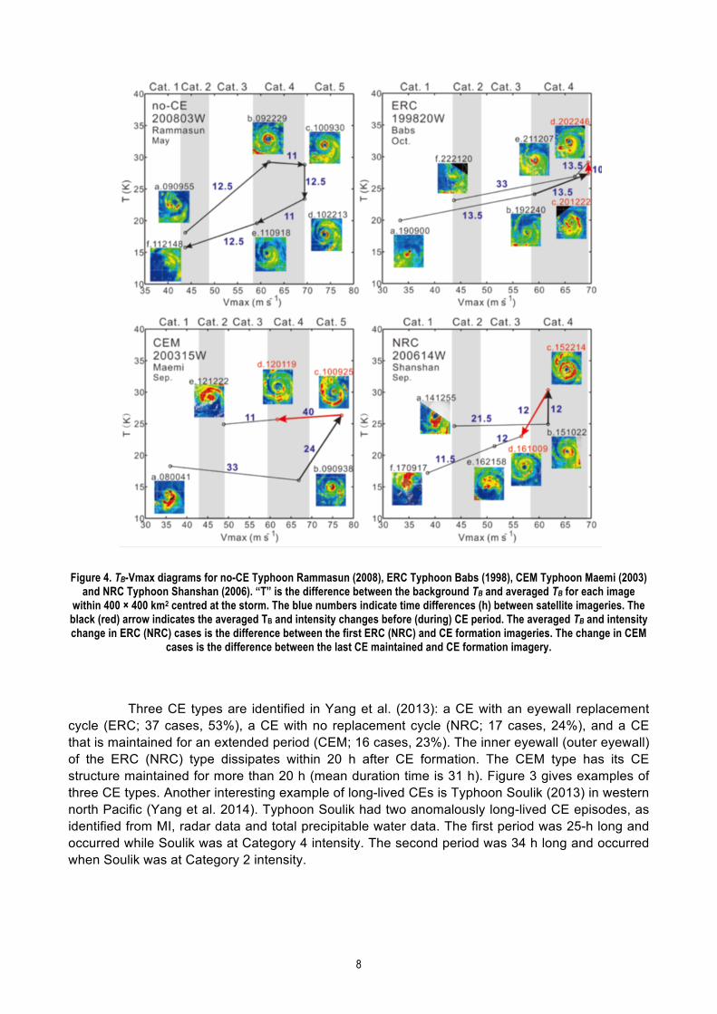
Figure 4. TB-Vmax diagrams for no-CE Typhoon Rammasun (2008), ERC Typhoon Babs (1998), CEM Typhoon Maemi (2003)

and NRC Typhoon Shanshan (2006). “T” is the difference between the background TB and averaged TB for each image within 400 × 400 km2 centred at the storm. The blue numbers indicate time differences (h) between satellite imageries. The black (red) arrow indicates the averaged TB and intensity changes before (during) CE period. The averaged TB and intensity change in ERC (NRC) cases is the difference between the first ERC (NRC) and CE formation imageries. The change in CEM

cases is the difference between the last CE maintained and CE formation imagery.

Three CE types are identified in Yang et al. (2013): a CE with an eyewall replacement cycle (ERC; 37 cases, 53%), a CE with no replacement cycle (NRC; 17 cases, 24%), and a CE that is maintained for an extended period (CEM; 16 cases, 23%). The inner eyewall (outer eyewall) of the ERC (NRC) type dissipates within 20 h after CE formation. The CEM type has its CE structure maintained for more than 20 h (mean duration time is 31 h). Figure 3 gives examples of three CE types. Another interesting example of long-lived CEs is Typhoon Soulik (2013) in western north Pacific (Yang et al. 2014). Typhoon Soulik had two anomalously long-lived CE episodes, as identified from MI, radar data and total precipitable water data. The first period was 25-h long and occurred while Soulik was at Category 4 intensity. The second period was 34 h long and occurred when Soulik was at Category 2 intensity.

9

Figure 5. The CE duration time in the western North Pacific and Atlantic

Structural and intensity changes of CE typhoons can be demonstrated using a TB-Vmax diagram (where Vm is the best track estimated intensity) for a time sequence of the intensity and convective activity (CA) relationship (e.g., Figure 4). The CA is indicated by the areal average TB contrast to the background TB in the 400-km square area of MI centered at the eye (CA≡−TBi−TB0). The background TB0 is calculated as the highest 5% of TB in the 400-km square area. The no-CE case is with an increase of intensity and CA before the peak and a decrease of intensity and CA afterward. On the other hand, the intensity of typhoons in the ERC and CEM cases weakens after CE formation, the CA is maintained or increases. In contrast, the CA weakens in the NRC cases. The NRC (CEM) cases typically have fast (slow) northward translational speeds and encounter large (small) vertical shear and low (high) sea surface temperatures. The CEM cases generally have a relatively high intensity (63 m s-1), and the moat size (61 km) and outer eyewall width (70 km) are approximately 50% larger than the other two categories. It appears that both the internal dynamics and environmental conditions are important in the CEM cases, while the NRC cases are heavily influenced by the environment. The ERC cases may be dominated by the internal dynamics due to more uniform environmental conditions. Finally, we note that the western North Pacific basin produces more cases of long duration CE TCs than the Atlantic basin (Figure 5). The CE duration time is the time period CE structure maintained as identified in MI by the objective method of Yang et al. (2013). Due to inadequate temporal resolution of MI, the duration of an entire ERC event (i.e., the time from the formation to the demise of CE structure) is not estimated. The long duration CEs in TCs deserve special attention for their structure and intensity change. III. Diagnosis of TC inner-core wind structure Another useful application for MI is in the diagnosis of TC wind structure. Rozoff et al. (2014b) present a method to estimate the inner-core wind structure from a variety of large retrospective developmental datasets. One dataset is a calibrated, developmental dataset of storm-centered passive MI (19, 37, and 85 GHz) data interpolated to standard cylindrical grids for Atlantic and Eastern Pacific TCs from 1995-2012. The other developmental datasets include a two-dimensional (2D) aircraft reconnaissance wind field analysis dataset described in Knaff et al. (2014) and the National Hurricane Center’s North Atlantic Hurricane Database (HURDAT; Jarvinen et al. 1984). A multiple linear regression model is designed to relate the azimuthal wavenumber 0-2 amplitudes and phases of the 2D wind fields to a variety of parameters, including the storm’s current intensity, position, and motion and the principle components of the 2D empirical orthogonal functions (EOFs) describing the structures in the MI dataset. This model thereby estimates the inner-core wind structure from MI imagery. The methodology is similar to the technique described

10

in Knaff et al. (2014), which uses IR data to estimate the wind field. An example of the MI-based method is provided in Figure 6.

Figure 6. (left) TMI polarization corrected temperatures (K) (37 GHz) of Hurricane Katrina (2005) at 0400 UTC 27

August. Missing data are seen in this image where there is land and in the northeast due to the region falling outside of the satellite swath. (right) Model diagnosed flight-level tangential winds (kt) associated with the 37-GHz MI at left.

b) Recommendations Given the many recent discoveries illustrating the significant benefits of using microwave imagery (MI) to identify important structural details of tropical cyclone (TC) inner-cores, research studies dedicated to using MI to diagnose and predict TC intensity and structure should continue to be supported. Moreover, research to operations should be facilitated in a timely manner to fully exploit current state-of-the-art forecasting techniques that benefit from the usage of MI. In the coming years, maintenance of a robust fleet of low-earth orbiting satellites with passive microwave sensors is essential for forecast operations to fully realize the benefits of including detailed TC structure information in analysis and forecast products. Many TCs across the globe are not routinely monitored by aircraft reconnaissance. Satellite data such as passive MI greatly ameliorate this limitation. SF 4a1.1.4 Estimating TC structure from coastal radar a) Recent progress Obtaining accurate TC structures before landfall is critical for forecasters and emergency managers. While convective structures of landfalling TCs can be obtained using radar reflectivity from a single radar, three-dimensional kinematic structures are best deduced from dual-Doppler analysis requiring two coastal radars. Typically, only a portion of a TC (e.g., a portion of inner core or rainband) can be deduced due to limited overlap of the Doppler domains (Yu and Cheng 2014). Taking advantage of the circular nature of the TC wind field, researchers have developed single-Doppler wind retrieval algorithms to derive the TC primary circulation and are able to estimate central pressure and the radial distribution of axisymmetric tangential winds from a single coastal radar (e.g., Lee et al. 1999; 2000; Harasti 2014). TC circulation centres can be determined within several kilometres accuracy by several different approaches using reflectivity (e.g., Chang et al. 2009) and Doppler velocity (e.g., Wood and Brown 1992; Lee and Marks 2000; Harasti and List 2005). A collection of these algorithms formed the basis of the VORTRAC (Vortex Objective Radar Tracking and Circulation) package that has been implemented at the NHC since 2008. Similar approaches have also been implemented in China and Taiwan.

11

The focus of research in recent years has been on improving individual algorithms in VORTRAC to obtain more accurate TC structure, and automating/streamlining procedures in VORTRAC for operational use. Recent progress has been made in the following three areas.

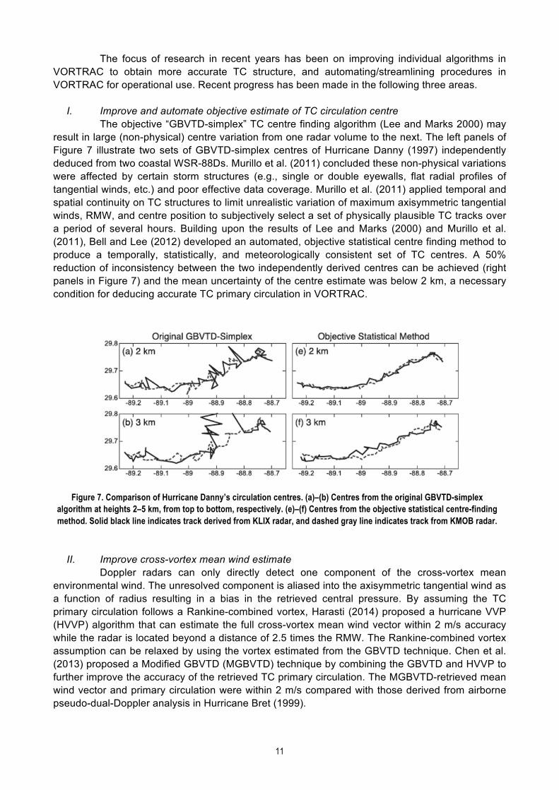
I. Improve and automate objective estimate of TC circulation centre The objective “GBVTD-simplex” TC centre finding algorithm (Lee and Marks 2000) may result in large (non-physical) centre variation from one radar volume to the next. The left panels of Figure 7 illustrate two sets of GBVTD-simplex centres of Hurricane Danny (1997) independently deduced from two coastal WSR-88Ds. Murillo et al. (2011) concluded these non-physical variations were affected by certain storm structures (e.g., single or double eyewalls, flat radial profiles of tangential winds, etc.) and poor effective data coverage. Murillo et al. (2011) applied temporal and spatial continuity on TC structures to limit unrealistic variation of maximum axisymmetric tangential winds, RMW, and centre position to subjectively select a set of physically plausible TC tracks over a period of several hours. Building upon the results of Lee and Marks (2000) and Murillo et al. (2011), Bell and Lee (2012) developed an automated, objective statistical centre finding method to produce a temporally, statistically, and meteorologically consistent set of TC centres. A 50% reduction of inconsistency between the two independently derived centres can be achieved (right panels in Figure 7) and the mean uncertainty of the centre estimate was below 2 km, a necessary condition for deducing accurate TC primary circulation in VORTRAC.

Figure 7. Comparison of Hurricane Danny’s circulation centres. (a)–(b) Centres from the original GBVTD-simplex

algorithm at heights 2–5 km, from top to bottom, respectively. (e)–(f) Centres from the objective statistical centre-finding method. Solid black line indicates track derived from KLIX radar, and dashed gray line indicates track from KMOB radar.

II. Improve cross-vortex mean wind estimate Doppler radars can only directly detect one component of the cross-vortex mean environmental wind. The unresolved component is aliased into the axisymmetric tangential wind as a function of radius resulting in a bias in the retrieved central pressure. By assuming the TC primary circulation follows a Rankine-combined vortex, Harasti (2014) proposed a hurricane VVP (HVVP) algorithm that can estimate the full cross-vortex mean wind vector within 2 m/s accuracy while the radar is located beyond a distance of 2.5 times the RMW. The Rankine-combined vortex assumption can be relaxed by using the vortex estimated from the GBVTD technique. Chen et al. (2013) proposed a Modified GBVTD (MGBVTD) technique by combining the GBVTD and HVVP to further improve the accuracy of the retrieved TC primary circulation. The MGBVTD-retrieved mean wind vector and primary circulation were within 2 m/s compared with those derived from airborne pseudo-dual-Doppler analysis in Hurricane Bret (1999).

12

III. Improve primary circulation estimate One of the major artifacts in Doppler radar observation in TC is velocity folding that needs to be de-aliased before use in the aforementioned algorithms. Wang et al. (2012) proposed the Gradient Velocity Track Display (GrVTD) technique that reformulates the GBVTD algorithm to directly ingest the aliased Doppler velocity field. By dealing with Doppler velocity gradient, GrVTD is more sensitive to the other data artifacts and data voids than the GBVTD technique, but can produce good results with adequate data coverage containing multiple velocity folds. b) Recommendation These recent research results provide great potential to further improve the performance of the VORTRAC package for future operational use in diagnosing the structures of landfalling TCs. Two fundamental limitations remain in the GBVTD techniques that need to be addressed in future research. First, the geometric distortion inherited in the GBVTD technique limits the analysis domain and phase aliasing of asymmetric structure beyond wavenumber one. Research is underway to formulate a Generalized VTD (GVTD) technique (Jou et al. 2008) that has a potential to alleviate the geometric distortion and solve for the cross-vortex mean wind vector. Second, these aforementioned algorithms still cannot resolve the asymmetric radial circulation. An improved physically based closure assumption will need to be developed in order to retrieve more complete TC circulation from coastal radars. On smaller spatial scales, the coastal WSR-88D radars were upgraded to dual polarization from 2011 – 2013, which will allow for improved diagnosis of the microphysical structure of TCs. The polarimetric upgrade should contribute to an improved understanding of the eyewall and rainband convective structure through a better characterization of hydrometeor types, particle size distributions, and identification of clutter and biological targets over the use of radar reflectivity products alone. These new WSR-88D products have only recently become available but are beginning to be explored (Van Den Broeke, 2013). Assimilating coastal radar data into numerical models has also been explored in recent years. Assimilating GBVTD-derived TC circulation into numerical models has been tested and shows encouraging results (e.g., Zhao et al. 2012a, b). This may be an area requires further research. SF4a1.1.5 Size and wind structure assessment from scatterometer data Scatterometry is an important tool for assessing TC structure, and these observations have been around since the mid-1990s. One of the truly successful scatterometers was the QuikSCAT instrument, which was launched on the QuikBird satellite in June 1999 and provided observations until its mission ended in November 2009. Hereafter, this entire set of instrument is referred to as QuikSCAT. QuikSCAT transmitted microwave pulses (in a continuous swath of 1800 km) down to the Earth's surface and then received the backscattered power that is related to surface roughness, which is highly correlated with the near-surface wind speed and direction on water surfaces. Hence, both wind speed and direction at the height of 10 m over the ocean surface can be estimated. It is noteworthy that QuikSCAT has a much larger swath of data than the currently operational Advanced Scatterometer (A-SCAT) that is on the MetOp –A and –B satellites and that this wider data swath is more conducive to TC structure studies. The post-processed 0.25° latitude by longitude gridded QuikSCAT data from the Remote Sensing Systems (RSS) database is used. These data are produced by RSS and sponsored by the National Aeronautics and Space Administration Ocean Vector Winds Science Team. Data are available at www.remss.com. RSS post-processed the QuikSCAT L2A data from the Jet Propulsion Laboratory, which was reprocessed in 2006 using Ku-2001 geophysical model function and passed through quality checks by comparing with the first-guess field of a numerical weather

13

prediction model so that the data are largely acceptable. Rain-free QuikSCAT winds below 20 m s-1 agree extremely well with buoys (Ebuchi et al. 2002). Using extremely limited validation data, those from 20 to 40 m s-1 are roughly verified to be within 10 m s-1 under rain-free conditions. It is well known that rain affects QuikSCAT and results in overestimated low winds or underestimated high winds when heavy rain is present. In TCs with winds weaker than 15 m s-1, the QuikSCAT winds in the presence of rain are often overestimated due to surface roughening and signal scattering. QuikSCAT winds within TCs above 20–30 m s-1 are often lower than actual storm speeds as the rain attenuates the radar signal (Atlas et al. 2001; Stiles and Yueh 2002; Brennan et al. 2009). Data selection is therefore important. In the past four years these data have been used to estimate TC size and to further our knowledge about how TC structure varies. Results of this work can be found in Lee et al. (2010), Chan and Chan (2012, 2013), and Chen et al. (2011). A well-documented method (Chan and Chan 2012) of how these data are used to create a TC size estimate is now described. a) Criteria for the selection of QuikSCAT data As QuikSCAT is a polar-orbiting satellite, its swath might not cover the entire circulation of a particular TC at a particular time. However, partial coverage still contains vital and unique information. To make the best use (i.e., minimizing noise and uncertainty while maximizing information content) of QuikSCAT data, the following criteria are used:

I. TC must be at tropical storm intensity or above (maximum sustained wind ≥ 17 m s-1)

II. The TC centre must be covered by the swath III. The distance between the TC centre and the edge of the swaths must be > 1° latitude IV. More than 50% of the TC circulation is covered by the swath V. The TC circulation should have no extensive wind-discontinuity problem

VI. Azimuthally-averaged wind speed profile must reach 17 m s-1 or above after filtering all rain- flagged data

VII. R17 is not close to any landmass VIII. Rain-flagged data are excluded While some of these criteria might seem somewhat subjective, such an approach minimizes the potential for large errors in TC size estimation. b) Estimation of TC size The size of a TC is defined as the average radial extent of gale-force surface winds (17 m s-1), R17 (i.e., also R34 elsewhere in this document). Azimuthally-averaged winds between 0.25° and 6.25° latitude from the centre are obtained by averaging the winds within each 0.25° latitude wide ring belt (0.125° ≤ r < 0.375° latitude radial area for the first ring belt). An azimuthal average is used in order to remove most of the asymmetry associated with TC motion (Shea and Gray 1973). To make sure that a reasonable value of the azimuthally-averaged wind in each ring belt can be obtained, the following criteria are also set. A missing value is set for any case failing either of these criteria.

I. The number of available (not rain-flagged) data points in each ring belt must be > 5 without considering the wind directions.

II. The fraction of available data points to total data points in each ring belt must be ≥ 0.5. It is assumed that a TC behaves like a Rankine vortex outside the radius of maximum winds, that is,

14

€

νθ r) = C( r−b (2)

where vθ is the tangential wind speed, r is the radial distance from the TC centre, and C and b are constants for a given profile. As the values of tangential winds and total winds are similar, especially at radii far away from the radius of maximum winds (Shea and Gray 1973), the total winds are assumed to be the same as the tangential winds. Six valid azimuthally-averaged winds with wind speeds closest to 17 m s-1 are then used to fit the vortex profile in (1) after taking the logarithm. The choice of 6 values (~ 1.5˚ latitude) is considered to be enough and reasonable to estimate R17. It should also be noted that the value of R17 from (1) is only considered to be acceptable if the innermost valid azimuthally-averaged wind is ≥ 17 m s-1. In other words, no extrapolation of TC size is allowed. c) Key results The mean TC size is found to be 2.13° latitude in the western North Pacific (WNP) and 1.83° latitude in the North Atlantic (NA). The correlation between size and intensity is weak. Seasonally, midsummer (July) and late-season (October) TCs are significantly larger in the WNP (Figure 8a) while the mean size is largest in September in the NA. The percentage frequencies of large TCs is also found to vary spatially and seasonally (Chan and Chan 2013) and were often determined by initial synoptic origin (e.g., wave vs. monsoon) (Lee et al. 2010). The latter finding suggests TCs deviate from a size that is determined during formation and has been confirmed by Knaff et al. (2014). In addition, the interannual variation of TC size in the WNP correlates significantly with the effect of El Niño over the WNP (Figure 8b) and TC lifetime (Figs. 8c, d). TC lifetime and seasonal subtropical ridge activity are shown to be potential factors that affect TC size. R17 values were also compared to JTWC estimates and generally showed a reluctance of JTWC (and likely other agencies) to estimate very large size TCs (Lee et al. 2010). Chen (2011) found that the early intensification stage is favourable for the occurrence of small (compact, lowest terrible) tropical cyclones, which also have a higher percentage of rapid intensification than larger TCs. Composite IR brightness temperature shows that compact tropical cyclones have highly axisymmetric convective structures with strong convection concentrated in a small region near the center. Changes in angular momentum (AM) transport in the upper and lower troposphere appear to be important factors that affect TC intensity and size, respectively. The change in TC intensity is positively related to the change in the upper-troposphere AM export, while the change in TC size is positively proportional to the change in the lower-troposphere AM import. An examination of the synoptic flow patterns associated with WNP TCs suggests that changes in the synoptic flow near the TC are important in determining the change in TC size, with developments of the lower-troposphere anticyclones flow (one to the east and one to the west) bordering the TC being favourable for TC growth (Figure 9a) and a weakening of the subtropical high to the southeast for TC size reduction (Figure 9b). A recurving TC tends to grow if the lower-tropospheric westerlies to its west increase (Figs. 9c,d). Moreover, northward TC movement is related to the change in TC size. For example, a higher northward-moving speed is found for a larger TC, which also agrees well with the AM transport concept (Chan and Chan 2013).

15

(a)

(b)

(c)

(d)

Figure 8. (a) Monthly means of TC size, (b) annual means of TC size and Niño 3.4 index, (c) monthly means of TC lifetime, and (d) annual means of TC lifetime over the WNP. Vertical bars represent the 95% confidence intervals of TC lifetime in the

t-distribution. Numbers above the x-axis indicate the number of cases and number of TCs (with parentheses).

16

(a) (b)

(c) (d)

Figure 9. (a) Composite of the changes in lower-tropospheric (850-hPa) synoptic flow of the growing TCs within 24 hours. (b) As in (a) but for the shrinking TCs. (c) As in (a) but for the recurving and growing TCs. (d) As in (a) but for the recurving

and shrinking TCs. Regions with dots denote that the changes in tangential or radial wind different from 0 have a confidence level higher than 90%.

More details can be found in Chan and Chan (2012, 2013), Lee et al. (2010) and Chen et al (2011). SF4a1.1.6 Size and wind field inferred from infrared satellite-based observations Much progress was made in the early 1970s to mid1990s with intensity estimation via the Dvorak Technique. While that work has led to the development of objective versions of the Dvorak technique (Olander and Velden 2007) that are being widely used to estimate TC intensity, few other infrared (IR)-based intensity methods have been attempted. In the last four years there have been renewed efforts to make improved use of routine IR satellite imagery. New techniques have been developed that estimate intensity, wind structure, and size.

17

One such method, the deviation angle variance technique (DAV-T,Piñeros et al. 2011; Ritchie et al. 2012), has been tested and has produced different error characteristics, but its overall performance is similar to subjective and objective Dvorak Techniques. The DAV-T quantifies the axisymmetric organization of cloud clusters via statistical analysis of the direction of the IR brightness temperature gradient. The gradient vectors are more aligned along radials pointing directly into or out from the center of a well-organized, developing cloud cluster compared with a weaker, more diffuse system, and thus greater cloud organization corresponds with lower DAV values. Observed DAV values for historical systems are used in conjunction with best track data to generate a sigmoid curve that correlates DAV with TC intensity, with successful application in the North Atlantic, western North Pacific, and eastern North Pacific basins (e.g., Ritchie et al. 2012; 2014). With respect to TC wind structure, new IR-based estimation methods come in two forms. The first method described here is a regression-based algorithm that uses DAV information contained in each IR image along with environmental information (such as SST) derived from the Statistical Hurricane Intensity Prediction Scheme (SHIPS) model (Dolling et al. 2014). Because the cloud structure provides an indicator for the low-level wind forcing of these clouds, the spatiotemporal information found in the corresponding DAV-T maps is compared with best track data within 3 hours of aircraft reconnaissance to create a multiple linear regression model. This model produces symmetric and asymmetric estimates of R34, R50, and R64. The errors associated with this method are shown in Figure 10.

Figure 10. Mean absolute error (MAE, nm) for: (a) northeast; (b) southeast; (c) southwest; and (d) northwest quadrants of the R34, R50, and R64 kt wind radii. Also included is the average testing (AT) of the 5 bins from the cross-validation

analysis.

In a similar vein, Knaff et al. (2014) present a method that relates TC-Vitals (intensity, latitude, motion) and principal components of direction-relative IR images to the azimuthal wavenumber 0 and 1 components of the direction-relative aircraft reconnaissance–based flight-level wind field. The Fourier components of the wind field are then used to reconstruct the winds at flight-level (e.g., Figure 11).

18

Figure 11. An illustration of the steps taken to estimate the wind field. The progression is from left to right and then top to

bottom. Imagery are mapped to a polar grid (1) and then rotated with respect to direction (2). Rotated imagery (via principle components), translation speed, latitude and intensity are then used to estimate the normalized wind field (3). The observed intensity is then applied to create a wind speed field (4). Finally the wind field is rotated back to its earth

relative directional component (5). This case is from Hurricane Ike (2008) on September 12 at 1145 UTC. The diagnosis of TC size can also be accomplished using IR information. A climatological study was undertaken to enable comparison of TC size among the different basins (Knaff et al. 2014). Here size is defined is the radius at which the TC wind field is indistinguishable from the background flow in a climatological environment (R5). R5 is calculated from the azimuthal mean brightness temperatures centered on the TC and the climatological decay rate beyond 500 km. Thirty years of R5 provided a clear picture of inter/intra-basin size changes and pointed to several possible causes for TC growth. R5 is also related to traditional TC size metrics including the radius of 34-, 50-, and 64-knot winds. About 40% of the variance of these parameters can be explained by R5 and current intensity. The relative ease of calculation of these IR measures of TC size, whether parametric or non-parametric, the objective nature of the methods, and a long history of IR imagery over TCs is likely to lead to statistical forecast tools in the near future. For example, because the DAV-T method utilizes geostationary satellite data, approximations of the wind radii can be produced on a half-hourly time scale with potential applications to data-sparse ocean regions and NWP model initialization.

19

A few recommendations come from this section. The first is that research efforts to use routine IR imagery to diagnose TC structure be supported by member countries. Similarly, research and operational communities should be encouraged to validate these methods. If validation proves that these methods are useful, research/operational funding should be encouraged to transition these methods to operational platforms where forecasters can have ready access to the information. SF4a1.2 Discussion and Recommendations In the last four years there have been a number of new methods and improvements to existing methods to diagnose elements of TC structure and to make those estimates inter-consistent. Some of these have been discussed in the previous sections. These techniques become more important as the forecast problems associated with track and intensity become more skillful. It is likely that in the coming years, that a greater emphasis on forecasting variations of TC structure will develop. At present the TC community is just beginning to study the physics of TC structure variation and these objective methods will provide the information need to develop this understanding and verify forecasts. With that need in mind we make the following recommendations.

I. Research emphasis should support the development a new physically-based closure assumption needed to retrieve more complete TC circulation from coastal radars, the examination of new dual-polarization radar to track eyewall features, and the regular assimilation of radar data in NWP.

II. Simple parametric-based vortex schemes should be transitioned to operations to help in TC-Vitals estimation and inter-consistency between routinely estimated parameters (e.g., ROCI, POCI, CP, Vm, RMW, etc.)

III. Structure parameters should routinely be extracted from NWP output, provided to the forecasters, and routinely verified. WMO should strive to ensure that methods of how this information is extracted should be standardized among TC forecast centres.

IV. WMO should encourage the development and deployment of scatterometers on future operational satellite platforms, possibly dual-frequency, to monitor marine winds and winds associated with TCs and complement other satellite information.

V. WMO should encourage the development and deployment of passive microwave radiometers and sounders on future operational satellite platforms.

VI. In the next four years, effort should be made to combine structure information derived from IR information along with traditional intensity and position fixes (e.g., Dvorak, DAV-T, etc.) when the same data is used for the intensity/position estimate. This will require including that information in the operational messages and database formats (ATCF, CXML etc…)

VII. Satellite-based methods that provide TC wind field structure estimates should be tested as an alternative approach for TC vortex initialization in regional hurricane and global models. This effort would offer the advantages of continuous reconnaissance and estimate of state variables without the difficulty of assimilation of cloudy/rainy radiances.

Acknowledgements The authors would like to thank their home institutions (U. of Hawaii, City Univ. of Hong Kong, Nat. Taiwan Univ., NCAR, U. Wisc., U. of Arizona, and NOAA) for the opportunity and time to work on this report.

20

Acronyms used in the report ATCF Automated Tropical Cyclone Forecast A-SCAT CE CEM

Advanced Scatterometer Concentric Eyewall CE Maintained

CP Central Pressure CXML Cyclone XML format DAV-T Deviation Angle Variance Technique DP ERC

Pressure Deficit Eyewall Replacement Cycle

GrVTD IR MI NRC NRL

Gradient Velocity Track Display Infrared Microwave Imagery No (Eyewall) Replacement Cycle Naval Research Laboratory

Penv Pressure of the environment POCI Pressure of the Outermost Closed Isobar QuikSCAT Scatterometer on the QuikBird Satellite R34/R17 in section SF4a1.1.5 Radius of 34 knot winds (Gale) R5 Radius of 5 knot wind at 850 hPa R50 Radius of 50 knot winds (Damaging) R64 RI

Radius of 64 knot winds (Hurricane) Rapid Intensification

RMW Radius of Maximum Winds SHB SHIPS SSM/I

Simplified Holland B Parameter Statistical Hurricane Intensity Prediction System Special Sensor Microwave/Imager

TC TMI TRMM

Tropical Cyclone TRMM Microwave Imager Tropical Rainfall Measuring Mission

Vm Maximum Wind of a TC VORTRAC Vortex Objective Radar Tracking and

Circulation References Atlas, R., and Coauthors, 2001: The effects of marine winds from scatterometer data on weather

analysis and forecasting. Bull. Amer. Meteor. Soc., 82, 1965–1990. Bell, M. M., and W.-C. Lee, 2012: Objective tropical cyclone center tracking using single Doppler

radar. J. Appl. Meteor., 51, 878-896. Brennan, M. J., C. C. Hennon, and R. D. Knabb, 2009: The operational use of QuikSCAT ocean

surface vector winds at the National Hurricane Center. Wea. Forecasting, 24, 621–645.

21

Chan, K. T. F., and J. C. L. Chan, 2012: Size and strength of tropical cyclones as inferred from QuikSCAT data. Mon. Wea. Rev., 140, 811–824.

Chan, K. T. F., and J. C. L. Chan, 2013: Angular momentum transports and synoptic flow patterns associated with tropical cyclone size change. Mon. Wea. Rev., 141, 3985–4007.

Chen D. Y-C, K.K.W. Cheung, and C-S Lee, 2011: Some implications of core regime wind structures in western North Pacific tropical cyclones. Wea. Forecasting, 26, 61-75.

Chen, X., K. Zhao, W.-C. Lee, B. J.-D. Jou, M. Xue, and P. R. Harasti, 2013: The improvement to the environmental wind and tropical cyclone circulation retrievals with Modified GBVTD (MGBVTD) technique. J. Appl. Meteor. Climatology, 52, 2493-2508.

Courtney, J., and J. A. Knaff, 2009: Adapting the Knaff and Zehr Wind-Pressure Relationship for operational use in Tropical Cyclone Warning Centres. Australian Meteorological and Oceanographic Journal, 58, 3, 167-179.

Davidson, N. E., Y. Xiao, Y. Ma, H. C. Weber, X. Sun, L. J. Rikus, J. D. Kepert, P. X. Steinle, G. S. Dietachmayer, C. C. F. Lok, J. Fraser, J. Fernon, and H. Shaik, 2014: ACCESS-TC: Vortex specification, 4DVAR initialization, verification, and structure diagnostics. Mon. Wea. Rev., 142, 1265–1289.

Dolling, K., E. A. Ritchie, and J. S. Tyo, 2014: A geostationary satellite technique to estimate tropical cyclone size. 31st Conference on Hurricanes and Tropical Meteorology. [ available on-line at https://ams.confex.com/ams/31Hurr/webprogram/Paper243452.html]

Ebuchi, N., H. C. Graber, and M. J. Caruso, 2002: Evaluation of wind vectors observed by QuikSCAT/SeaWinds using ocean buoy data. J. Atmos. Oceanic Technol., 19, 2049–2062.

Harasti, P. R. and R. List, 2005: Principal Component Analysis of Doppler Radar Data. Part I: Geometric Connections between Eigenvectors and the Core Region of Atmospheric Vortices. J. Atmos. Sci., 62, 4027–4042.

Harasti, P. R., 2014: An expanded VVP technique to resolve primary and environmental circulations in hurricanes. J. Atmos. Oceanic Technol., 31, 249-271.

Harnos, D. S., and S. W. Nesbitt, 2011: Convective structure in rapidly intensifying tropical cyclones as depicted by passive microwave measurements. Geophys. Res. Letts., 38, L07805, doi:10.1029/2011GL04010.

Hart R.E., 2003: A cyclone phase space derived from thermal wind and thermal asymmetry. Mon. Wea. Rev., 131, 585–616.

doi: http://dx.doi.org/10.1175/1520-0493(2003)131<0585:ACPSDF>2.0.CO;2 Hawkins, J. D., T. F. Lee, F. J. Turk, C. Sampson, J. Kent, and K. Richardson, 2001: Real-time

Internet distribution of satellite products for tropical cyclone reconnaissance. Bull. Amer. Meteor. Soc., 82, 567–578.

Hawkins, J. D., and M. Helveston, 2004: Tropical cyclone multiple eyewall characteristics. Preprints, 26th Conf. on Hurricane and Tropical Meteorology, Miami, FL, Amer. Meteor. Soc., P1.7.

Hawkins, J. D., M. Helveston, T. F. Lee, F. J. Turk, K. Richardson, C. Sampson, J. Kent, and R. Wade, 2006: Tropical cyclone multiple eyewall characteristics. Preprints, 27th Conf. on Hurricane and Tropical Meteorology, Monterey, CA, Amer. Meteor. Soc., 6B.1.

Hawkins, J., and C. Velden, 2011: Supporting meteorological field experiment missions and postmission analysis with satellite digital data and products. Bull. Amer. Meteor. Soc., 92, 1009-1022.

Hendricks, E. A., M. S. Peng, B. Fu, and T. Li, 2010: Quantifying environmental control on tropical cyclone intensity change. Mon. Wea. Rev., 138, 3243-3271.

Holland, Greg J., 1980: An analytic model of the wind and pressure profiles in hurricanes. Mon. Wea. Rev., 108, 1212–1218.

22

Jarvinen, B. R., C. J. Neumann, and M. A. S. Davis, 1984: A tropical cyclone data tape for the North Atlantic basin, 1886-1983: Contents, limitations, and uses. NOAA Tech. Memo. NWS NHC 22, 21 pp.

Jiang, H., and E. M. Ramirez, 2013: Necessary conditions for tropical cyclone rapid intensification as derived from 11 years of TRMM data. J. Climate, 26, 6459-6470.

Kaplan, J., M. DeMaria, and J. A. Knaff, 2010: A revised tropical cyclone rapid intensification index for the Atlantic and eastern North Pacific basins. Wea. Forecasting, 25, 220-241.

Kieper, M. E., and H. Jiang, 2012: Predicting tropical cyclone rapid intensification using the 37 GHz ring pattern identified from passive microwave measurements. Geophys. Res. Letts., 39, L13804, doi:10.1029/2012GL052115.

Knaff, J.A., S.P. Longmore, R.T DeMaria, D.A. Molenar, 2014: Improved Tropical Cyclone Flight-Level Wind Estimates Using Routine Infrared Satellite Reconnaissance. J. App. Meteor. Climate. (in press).

Knaff, J. A., P. J. Fitzpatrick, C. R. Sampson, Y. Jin, and C.M. Hill, 2011: Simple diagnosis of tropical cyclone structure via pressure gradients. Wea. Forecasting. 26, 1020-1031.

Kummerow, C., W. Barnes, T. Kozu, J. Shiue, and J. Simpson, 1989: The Tropical Rainfall Measuring Mission (TRMM) sensor package. J. Atmos. Oceanic Technol., 15, 809–817.

Kuo, H.-C., C.-P. Chang, Y.-T. Yang, and H.-J. Jiang, 2009: Western North Pacific typhoons with concentric eyewalls. Mon. Wea. Rev., 137, 3758-3770.

Lee C-S, K.K.W. Cheung, W-T. Fang, and R. L. Elsberry, 2010: Initial maintenance of tropical cyclone size in the western North Pacific. Mon. Wea. Rev., 138, 3207-3223.

Lee, W.-C., and M. M. Bell, A. M. Forester, X. Tang, and P. R. Harasti, 2014: Intensity guidance and center tracking for landfalling tropical cyclones by VORTRAC. 31st Conference on Hurricanes and Tropical Meteorology, San Diego, CA, 30 March – 4 April.

Marchok, T.P., 2002: How the NCEP tropical cyclone tracker works. Preprints, 25th Conf. on Hurricanes and Tropical Meteorology, San Diego, CA, Amer. Meteor. Soc., 21-22.

McGuaghey, G., E. J. Zipser, R. W. Spencer, and R. E. Hood, 1996: High-resolution passive microwave observations of convective systems over the tropical Pacific Ocean. J. Appl. Meteorol., 35, 1921-1947.

Molinari, J., and D. Vollaro, 2010: Rapid intensification of a sheared tropical storm. Mon. Wea. Rev., 138, 3869-3885.

Murillo, S. T., W.-C. Lee, M. M. Bell, F. D. Marks, P. P. Dodge, G. M. Barnes, 2011: Intercomparison of GBVTD-retrieved circulation centers and structures of Hurricane Danny (1997) from two coastal WSR-88Ds. Mon. Wea. Rev., 139, 153-174.

Nguyen, L., and J. Molinari, 2012: Rapid intensification of a sheared, fast-moving hurricane over the Gulf Stream. Mon. Wea. Rev., 140, 3361-3378.

Pendergrass, A. G., and H. E. Willoughby, 2009: Diabatically induced secondary flows in tropical cyclones. Part I: Quasi-steady forcing. Mon. Wea. Rev., 137, 805-821.

Piñeros, M.F., E. A. Ritchie, and J. S. Tyo, 2011: Estimating Tropical Cyclone Intensity from Infrared Image Data. Wea. Forecasting,26, 690–698. doi: http://dx.doi.org/10.1175/WAF-D-10-05062.1

Powell, M. D., S. H. Houston, L. R. Amat, and N Morisseau-Leroy, 1998: The HRD real-time hurricane wind analysis system. J. Wind Engineer. and Indust. Aerodyn. 77&78, 53-64

Ritchie E. A., G. Valliere-Kelley, M. F. Piñeros, and J. S. Tyo, 2012: Tropical Cyclone Intensity Estimation in the North Atlantic Basin Using an Improved Deviation Angle Variance Technique. Wea. Forecasting, 27, 1264–1277.

23

Ritchie, E. A., K. M. Wood, O. G. Rodríguez-Herrera, M. F. Piñeros, and J. S. Tyo, 2014: Satellite-derived tropical cyclone intensity in the North Pacific Ocean using the deviation-angle variance technique. Wea. Forecasting, 29, 505-516.

Rogers, R., P. Reasor, and S. Lorsolo, 2013: Airborne Doppler observations of the inner-core structural differences between intensifying and steady-state tropical cyclones. Mon. Wea. Rev., 141, 2970-2991.

Rozoff, C. M., C. S. Velden, J. Kaplan, J. P. Kossin, and A. J. Wimmers, 2014a: Improvements in the probabilistic prediction of tropical cyclone rapid intensification with passive microwave observations. Wea. Forecasting, submitted.

Rozoff, C. M., J. A. Knaff, and M. Amin, 2014b: Estimating tropical cyclone wind structure from passive microwave imagery. Manuscript in preparation.

Sampson, C. R., and A. J. Schrader, 2000: The automated tropical cyclone forecasting system (version 3.2). Bull. Amer. Meteor. Soc., 81, 1231–1240.

Shea, D. J., and W. M. Gray, 1973: The hurricane's inner core region. I. Symmetric and asymmetric structure. J. Atmos. Sci., 30, 1544–1564.

Sitkowski, M., J. Kossin, and C. M. Rozoff, 2011: Intensity and structure changes during hurricane eyewall replacement cycles. Mon. Wea. Rev., 139, 3829-3847.

Spencer, R. W., H. M. Goodman, and R. E. Hood, 1989: Precipitation retrieval over land and ocean with the SSM/I: Identification and characteristics of the scattering signal. J. Atmos. Oceanic Technol., 6, 254-273.

Stiles, B. W., and S. Yueh, 2002: Impact of rain on spaceborne Ku-band scatterometer data. IEEE Trans. Geosci. Remote Sens., 40, 1973–1983.Tallapragada, V., and Co-authors, 2014: Hurricane Weather Research and Forecasting (HWRF) Model: 2014 Scientific Documentation. pp 76-94. [ available online at:

http://www.dtcenter.org/HurrWRF/users/docs/scientific_documents/HWRFv3.6a_ScientificDoc.pdf ]

Van Den Broeke, M. S., 2013: Polarimetric Radar Observations of Biological Scatterers in Hurricanes Irene (2011) and Sandy (2012). J. Atmos. Oceanic Technol., 30, 2754–2767.

Vigh, J. L., and W. H. Schubert, 2009: Rapid development of the tropical cyclone warm core. J. Atmos. Sci., 66, 3335-3350.

Wang, M., K. Zhao, W.-C. Lee, B. J.-D. Jou, and M. Xue, 2012: The Gradient Velocity Track Display (GrVTD) Technique for Retrieving Tropical Cyclone Primary Circulation from Aliased Velocities Measured by Single Doppler Radar. J. Atmos. Oceanic Technol., 29, 1026-1041.

Weng, F., and N. C. Grody, 1994: Retrieval of cloud liquid water using the special sensor microwave imager (SSM/I). J. Geophys. Res., 99, 25535-25551.

Yang, Y.-T., H.-C. Kuo, E. A. Hendricks, M. S. Peng, 2013: Structural and Intensity Changes of Concentric Eyewall Typhoons in the Western North Pacific Basin. Mon. Wea. Rev., 141, 2632-2648.

Yang, Y. T., E. Hendrick, H. C. Kuo, and M. Peng, 2014: Long-lived Concentric Eyewalls in Typhoon Soulik (2013). Mon. Wea. Rev., 142, 3365-3371.

Zagrodnik, J., and H. Jiang, 2014: Rainfall, convection, and latent heating distributions in rapidly intensifying tropical cyclones. J. Atmos. Sci., 71, 2789-2809.

Zhao, K., M. Xue, and W.-C. Lee, 2012: Assimilation of GBVTD-Retrieved winds from single-Doppler radar for short-term forecasting of super Typhoon Saomai (0608) at landfall. Quar. J. Royal Meteor. Soc. 138, 1055-1071.

Zhao, K., X. Li, M. Xue, B. J.-D. Jou, and W.-C. Lee, 2012: Short-term forecasting through intermittent assimilation of data from Taiwan and mainland China coastal radars for Typhoon Meranti (2010) at landfall. J. Geophys. Res., 117, D6, doi:10.1029/2011JD017109.