spe 98012 reservoir characterization using intelligent ... · 2 reservoir characterization using...

Copyright 2005, Society of Petroleum Engineers This paper was prepared for presentation at the 2005 SPE Eastern Regional Meeting held in Morgantown, W.V., 14–16 September 2005. This paper was selected for presentation by an SPE Program Committee following review of information contained in a proposal submitted by the author(s). Contents of the paper, as presented, have not been reviewed by the Society of Petroleum Engineers and are subject to correction by the author(s). The material, as presented, does not necessarily reflect any position of the Society of Petroleum Engineers, its officers, or members. Papers presented at SPE meetings are subject to publication review by Editorial Committees of the Society of Petroleum Engineers. Electronic reproduction, distribution, or storage of any part of this paper for commercial purposes without the written consent of the Society of Petroleum Engineers is prohibited. Permission to reproduce in print is restricted to a proposal of not more than 300 words; illustrations may not be copied. The proposal must contain conspicuous acknowledgment of where and by whom the paper was presented. Write Librarian, SPE, P.O. Box 833836, Richardson, TX 75083-3836, U.S.A., fax 01-972-952-9435.

Abstract Today, the major challenge in reservoir characterization is integrating data coming from different sources in varying scales, in order to obtain an accurate and high-resolution reservoir model. The role of seismic data in this integration is often limited to providing a structural model for the reservoir. Its relatively low resolution usually limits its further use. However, its areal coverage and availability suggest that it has the potential of providing valuable data for more detailed reservoir characterization studies through the process of seismic inversion. In this paper, a novel intelligent seismic inversion methodology is presented to achieve a desirable correlation between relatively low-frequency seismic signals, and the much higher frequency wireline-log data. Vertical seismic profile (VSP) is used as an intermediate step between the well logs and the surface seismic. A synthetic seismic model is developed by using real data and seismic interpretation. In the example presented here, the model represents the Atoka and Morrow formations, and the overlying Pennsylvanian sequence of the Buffalo Valley Field in New Mexico. Generalized regression neural network (GRNN) is used to build two independent correlation models between; 1) Surface seismic and VSP, 2) VSP and well logs. After generating virtual VSP’s from the surface seismic, well logs are predicted by using the correlation between VSP and well logs. The values of the density log, which is a surrogate for reservoir porosity, are predicted for each seismic trace through the seismic line with a classification approach having a correlation coefficient of 0.81. The same methodology is then applied to real data taken from the Buffalo Valley Field, to predict interwell gamma ray and neutron porosity logs through the seismic line of interest. The same procedure can be applied to a complete 3D seismic block to obtain 3D distributions of reservoir properties with less uncertainty than the geostatistical estimation methods. The intelligent seismic inversion method should help to increase the success of

drilling new wells during field development. Introduction Reservoir characterization requires building a spatial model of the reservoir by using appropriate data gathered from previous studies. This spatial model is then used in flow simulators, which can predict reservoir performance. An accurate and reliable reservoir characterization study is indispensable in reservoir management. The major challenge in today’s reservoir characterization is to integrate all different kinds of data to obtain an accurate and high-resolution reservoir model. The concept of data analysis forms the basis of reservoir characterization. Uncertainty, unreliability, and large variety of scales due to the different origins of the data must be taken into consideration. Together with the immense size of the data sets that must be dealt with, these issues bring complex problems, which are hard to address with conventional tools. That’s why unconventional computation tools have gained much interest in data analysis in recent years. Among those modern tools; intelligent systems, which mimic the mechanism of the human mind, are a way of dealing with imprecision and partial truth1. It should not surprise us that using intelligent systems in reservoir characterization studies has become a widely-used method in the petroleum engineering literature. Some previous intelligent reservoir characterization applications include, but are not limited to, synthetic log generation2,3,4, permeability estimation from logs5,6, and predicting bulk volume of oil7.

Let us consider different types of data used in reservoir characterization: core samples provide very high resolution information about the reservoir (fraction of inches), while seismic data have a resolution in tens of feet, and well logs have in one of inches. Because of its low resolution, seismic data is routinely used only to attain a structural view of the reservoir. On the other hand, unlike core samples or well logs, which are only available at isolated localities of a reservoir, seismic data frequently provides 3D coverage over a large area. Because of this areal coverage, researchers have always aimed to use seismic data in reservoir description. Inverse modeling of reservoir properties from the seismic data is known as seismic inversion in the literature. The process presented in this paper includes modeling of the well logs from seismic data, which is also an inverse modeling process (Figure 1). This approach attracts a lot of interest and is very important because of the necessary shift from exploration to development of existing fields8. Seismic inversion has been applied by several authors with different approaches. Hampson et al.8 and Leiphart and Hart9

SPE 98012

Reservoir Characterization Using Intelligent Seismic Inversion Emre Artun, SPE, West Virginia University; Shahab D. Mohaghegh, SPE, West Virginia University; Jaime Toro, West Virginia University; Tom Wilson, West Virginia University; Alejandro Sanchez, Anadarko Petroleum Corporation

2 Reservoir Characterization Using Intelligent Seismic Inversion SPE 98012

have compared different techniques such as multiple linear regression, backpropagation and probabilistic neural networks. They have predicted porosity logs from seismic attributes and both have suggested using probabilistic neural networks in this type of problems considering its mathematical simplicity and success.

Balch et al.10 have used fuzzy ranking to see which type of seismic attribute is related to the target reservoir property. They have modeled correlations between those selected attributes and porosity, water saturation and net pay thickness by using a backpropagation neural network. Chawathe et al.11 used neural networks to predict gamma ray log from seismic attributes; amplitude, phase, frequency, reflection strength, and quadrature. However, they have used higher-resolution crosswell seismic data instead of surface seismic as a new approach. Soto and Holditch12 have used the same types of attributes from surface seismic to predict the gamma ray log with neural networks.

Reeves et al.13 introduced a new methodology, which divides the whole seismic inversion problem into two parts. They have considered cross-well tomography as an intermediate step in their procedure, after finding a correlation between surface seismic and cross-well seismic. They have suggested producing virtual cross-well seismic data, before dealing with logs. Giving Chawathe et al.’s11 work as an example, they stated that well logs can easily be predicted from virtual cross-well seismic data. According to the authors, using crosswell seismic as an intermediate scale data can provide improved vertical resolution, increase constraints and reduce the uncertainty of reservoir description.

In this study, a similar methodology is followed. Instead of cross-well seismic which is rather hard to obtain, vertical seismic profile (VSP) is incorporated into the study as the intermediate scale data. This is due to the fact that VSP is available more frequently, and is less expensive to obtain than cross-well tomography. It is a common type of data that can be found in many fields.

Together with the integration of a third type of data, another unique feature of this study was developing and integrating a synthetic model to the research, before dealing with real data. Having a synthetic model that we had full control of gave us the opportunity to develop and test the proposed methodology better before applying it to real data. Our synthetic model represents the gas-producing Atoka and Morrow formations and the overlying Pennsylvanian sequence in the Buffalo Valley Field in New Mexico. Surface seismic and VSP responses of this model are computed. Artificial neural networks are used to develop two independent correlation models between; 1) Surface seismic and VSP, 2) VSP and well logs. Density log has been selected as the target log, and is predicted from the seismic line. In the second case, seismic field data have been used to predict gamma ray and neutron porosity distributions through a seismic section.

In the following sections a theoretical background, which includes brief explanations of seismic surveys and artificial neural networks -under the light of the methodology of this study- are included. Then, the methodologies followed in the synthetic and the field cases are presented. After that, the results and their discussions are followed by conclusions.

Theoretical Background Seismic Surveys. The seismic method is the most widely used tool in the exploration of hydrocarbon reservoirs. It is useful for obtaining a structural view of the subsurface geology. The basic theory of the seismic method is based on the movements of signals through the subsurface. Reflection method is the most widely used seismic method, which is useful in identifying formation tops. A seismic trace is the response of a single seismic detector to the seismic energy propagation through the earth. If these traces are displayed side-by-side, then it is called a seismic record. A processing stage comes after obtaining a seismic record, to enhance the signal, to minimize the noise and increase the resolution. These processed images are than compiled together to produce the final output of the seismic survey: a seismic section14. Vertical seismic profiling (VSP) differs from conventional seismic surveys in the location of signal receivers. In VSP surveys, the receivers are located in the borehole instead of at the earth’s surface. Because the earth acts as a low-pass filter, placing of the receivers at depth reduces the distance that the signal has to travel through the earth, thus yielding higher frequency (higher resolution) data. VSP surveys are very similar to velocity surveys in terms of where the sources and receivers are located. However, they differ from each other with two issues14: 1) The distance between geophone recording depths (smaller in VSP, every 15-40 meters) 2) Collection of information (Only first break times are collected in velocity surveys. In VSP, upgoing and downgoing events are also collected for several seconds.) Seismic attributes are all the information obtained from seismic data, either by direct measurements or by logical or experience-based reasoning15. The attributes used in this study can be briefly defined as; Amplitude: Measure of the strength of the reflected signal. Indicates changes in physical properties of various lithological entities. It can sometimes be used to detect gas presence11. Hilbert Transform: This amounts to a 90-degree phase rotation. Amplitude and Hilbert transform are combined as Cartesian components of a trace signal16. Instantaneous Phase: Phase angles range from -180 degrees to +180 degrees. Envelope and phase are combined as polar components of a trace signal16. Average Energy: This attribute integrates the envelope between paraphase events. It highlights stratigraphic detail through energy fluctuations across traces. Values are in degrees16. Envelope: Represents the reflection strength. The envelope is independent of the phase and it relates directly to the acoustic impedance contrasts16. Frequency: This attribute describes how long it takes the phase to complete 360 degrees of rotation16. Paraphase: This attribute is the instantaneous phase with the predictable trend removed. As such, it assists visualizing the structural picture because phase tracks geologic boundaries16. Artificial Neural Networks. Artificial neural networks (ANN) can be broadly defined as information processing systems that mimic the human mind as a mathematical model

SPE 98012 Artun, Mohaghegh, Toro, Wilson & Sanchez 3

representation of the biological neural networks. ANN have gained an increasing popularity in different fields of engineering in the past few decades, because of their capability of extracting complex and non-linear relationships. Their mechanism is based on the following assumptions17: 1) Information processing occurs in many simple elements that are called neurons (processing elements). 2) Signals are passed between neurons over connection links. 3) Each connection link has an associated weight, which, in a typical neural network, multiplies the signal being transmitted. 4) Each neuron applies an activation function (usually non-linear) to its net input to determine its output signal. Figure 2 shows a typical neuron (processing element). Outputs (In) coming from another neuron are multiplied by their corresponding weights (Wn), and summed up. An activation function is then applied to the summation, and the output of that neuron is now calculated and ready to be transferred to another neuron18. There are many different types of neural network architectures and algorithms available. In this study, a generalized regression neural network (GRNN) is used. GRNN is a modification to probabilistic neural network that has been suggested by authors, who have studied seismic inversion8,9. GRNN has also been successfully used in geological pattern recognition applications such as synthetic log generation10 and total organic carbon content prediction from logs19. Besides, GRNN has been used in finding a correlation between cross-well seismic and surface seismic13,20. Huang et al.19 described GRNN as an easy-to-implement tool, which has efficient training capabilities, and the ability to handle incomplete patterns. Generalized Regression Neural Network. Introduced by Specht21 in 1991, GRNN is a one-pass learning algorithm with a highly parallel structure. It is a memory-based network, which provides estimates of continuous variables, and converges to the underlying regression surface. This approach is freed from the necessity of assuming a specific functional form. Instead, the appropriate form is expressed as a probability density function (pdf), which can be determined from the observed data. General regression uses y (a scalar random variable), the X (a particular measured value of a vector random variable x), and the non-parametric estimator of the joint probability density function f(x, y). After defining the scalar Euclidian distance function, Di

2; )()(2 iTi

i XXXXD −−= (1) performing the integrations results with the following:

∑

∑

=

=

⎟⎟⎠

⎞⎜⎜⎝

⎛−

⎟⎟⎠

⎞⎜⎜⎝

⎛−

=n

i

i

n

i

ii

D

DY

XY

1

2

1

2

2exp

2exp

)(ˆ

σ

σ (2)

In order to define it in a simpler mathematical form, (4) is

proposed instead of (2), which has given similar results. Instead of the Euclidian distance, it uses the city block distance, Ci;

∑=

−=p

j

ijji XXC

1

(3)

∑

∑

=

=

⎟⎟⎠

⎞⎜⎜⎝

⎛−

⎟⎟⎠

⎞⎜⎜⎝

⎛−

=n

i

i

n

i

ii

C

CY

XY

1

1

exp

exp)(ˆ

σ

σ (4)

The estimate Y(X) is defined as a weighted average of the observed values, Yi, where each observed value is weighted exponentially according to its Euclidian or city block distance21. σ is the smoothing factor, and optimum smoothing factor is determined after several runs according to the mean-squared error of the estimate, which must be kept at minimum. This process is referred to as the training of the network. If a number of iterations pass with no improvement in the mean-squared error, that smoothing factor is determined as the optimum one for that data set. In the production phase, that smoothing factor is applied to data sets that the network has not seen before. While applying the network to a new set of data, increasing the smoothing factor would result in decreasing the range of output values. GRNN is known to be particularly useful in approximating continuous functions, such as logs, or other types of geological patterns. It may have multidimensional input, and it will fit multidimensional surfaces through data22. It is a three-layer network. In the hidden layer, there must be one hidden neuron for each training pattern. Case 1: Synthetic Model Study Description of the model. The model was developed using Struct, a modeling package in the Geographix DiscoveryTM Suite of Landmark Graphics®. It is a comparative example of the stratigraphic section of the Buffalo Valley Field, which includes Atoka and Morrow formations together with the overlying Pennsylvanian sequence, where stratigraphic complexity increases with depth. It is developed by using a forward modeling process, which has simulated straight rays traveling from the surface and avoiding diffraction at interfering events. The model has been defined with properties like thickness, geometry, lateral distribution, density and interval velocity of the rocks, which were gathered from the actual data set23: Horizontal dimension - 4.9 mi (7.9 km), equivalent to the dimension of the 3D seismic survey. Vertical dimension - Real depth - approximately 7000 ft; and thickness of the sequence – approximately 2000 ft. This data was measured from well logs. Geometry of the sand channels and sand/limestone layers - After considering the well log interpretation and seismic visualization, channels and layers were defined as having thicknesses between 10 and 80 ft. Density and interval velocity of shales and sand bodies - The average density and velocity values were derived from well logs are shown in Table 1.


Surface Seismic and VSP-Derived Models. Two separate models were obtained by extracting wavelets from actual surface seismic and VSP for the time window of the Atoka and Morrow formations. The synthetic surface seismic response was computed by using a wavelet derived from the zone of interest in line 1034 of the 3D surface seismic data, and the synthetic VSP response (Figure 3) was computed by using a Butterworth wavelet derived from line 2064 of the 3D VSP with a larger bandwidth. The properties of the wavelets used for each case are shown in Table 2. The tuning thickness provides a measure of the vertical resolution limit of the seismic data, which can be calculated with the relationship; VR = v/4f (5) where; VR is the vertical resolution in ft/(sec × Hz), v is the interval velocity in ft/sec and f is the dominant frequency in Hz. 1% noise were introduced to the model during the computations23. In the model, the geological complexity increases with depth. The positive amplitudes (blue in Figure 3) are produced at the top of the carbonates, reflecting the interface between an overlying weak acoustic impadance rock (shales, layers in white) and an underlying high acoustic impadance (carbonates). Negative amplitude is produced due to the interface between the strong acoustic impedance carbonate, and the underlying weak impedance shale23. Model Output. The model is basically a seismic line of 100 traces, which includes three wells at traces 20, 50 and 80 with the well at trace 50 having a VSP survey. These wells had well logs of density and acoustic velocity. The available data after developing the model were; 1) Surface seismic and vertical seismic profile responses in

the form of the following seismic attributes: − Trace amplitude − Average energy − Trace envelope − Instantaneous frequency − Hilbert transform − Paraphase − Instantaneous phase

2) Density and acoustic velocity distributions.

Methodology. The methodology in this study includes two major steps of correlation as proposed (Figure 1); 1) Correlation of surface seismic with VSP; 2) Correlation of VSP with well logs.

The data used is within the interval 0.8-1.124 seconds (6600-9000 ft.), as it represents a major exploration target in the area. Above this interval, there is seismic noise that was ignored as input data. In the following section, these two steps of correlation will be explained in details.

Step 1: Correlation of Surface Seismic with VSP: An effort was made to find a correlation between surface seismic attributes and VSP attributes. First, the model was visualized:

cross-sectional distributions of density, acoustic velocity and seismic attributes for both surface seismic and VSP were plotted. The main aim was to determine the most appropriate portion of the synthetic data set that should be used in training of the network. The success of a neural network model depends strongly on the way it is trained. Thus, the training data set must be representative of the geological complexity of the area being modeled. Only then, one can obtain successful results in the prediction phase. For this purpose, an effort was made to identify special geological features that can be useful in training the neural network. These include: edges of sand channels, extreme value points, and unique geological structures. In this particular case, those kinds of features could be found mostly in the central part of the synthetic seismic section. After several tests, we decided to use data of traces 32 and 57 (Figure 4). Because of the limitation in optimum number of data rows, only two traces were used for training. The network structure used in training is shown in Figure 5-a. As shown, data of traces 32 and 57 were used to predict a VSP attribute from time and seven available surface seismic attributes. At the end, seven separate prediction models have been developed for seven attributes. After having confidence of the prediction abilities of these models, they were applied to the whole seismic line to obtain network-predicted distributions of all the available seismic attributes. These attributes were then plotted in order to compare them with the actual ones. Step 2: Correlation of VSP with Well Logs: The second step of the correlation was deriving log properties from the neural network-derived VSP data. Since trace 50 is the trace which includes all of the data that we are dealing with (i.e. surface seismic, VSP and well logs), this trace was used to develop the model for this part of the correlation. The density log was selected as the target log. When one looks at the density log of trace 50, one can clearly see that there are a few different averaged values of density (Figure 6), which have been later defined as classes. Each of these classes actually represents a different type of rock layer defined in the model. Finally, instead of using actual values of density, it was decided to use these classes as the target values. By doing this, we have changed the nature of the neural modeling to one of classification. Classification networks are sometimes simpler than networks that are built to predict continuous values. In the initial trial; classes were defined as (Figure 6);

- Class 1: ρ ≈ 1.9 g/cc - Class 2: ρ ≈ 2.3 g/cc - Class 3: ρ ≈ 2.65 g/cc

Thus, the network structure was like the one in Figure 5-b.

All of the VSP attributes and time were used as inputs to predict one of the density classes. Case 2: Field Study (B. Valley Field, New Mexico) Available data. The following data were used in this study23: 1) A 3D seismic survey, loaned by WesternGeco for this

study, covering an area of 24 mi2 with a vibroseis source,


sweep frequencies ranging from 8 to 98 Hz, and a sweep length of 17 seconds.

2) A vertical seismic profile volume, with a two-LRS-315 vibrators source, covering an area of approximately 3.5 mi2 in the southeast corner of the area.

3) Logs from around 40 wells were available as either paper or electronic copies. Available types of logs included gamma ray, neutron, density, sonic, spontaneous potential, and resistivity. Paper copies have been scanned, and then digitized together with other available electronic copies. Average total depth of those wells were ranging from 8000 to 9000 ft, intersecting the Atoka and Morrow formations.

Unfortunately, not all of the available well logs were of high visual quality. That made them hard to accurately digitize. It is a proven fact that quality of the data has an important role in building reliable neural network models. Reasonable amount of noise in the data is acceptable, and even useful for a more realistic model. However, it is impossible to rely on a model, which has been built with unreliable data. Rolon’s study4 clearly states this fact, by comparing two similar studies with well log data having different levels of quality. Given these issues, the digitized log files were evaluated and selected for neural network design based on overall quality, to avoid building poor prediction models. Only good quality logs were used. Within the context of log quality and distribution, and the location of the VSP well, a seismic line (Figure 7) was extracted from the 3D survey area for use in the neural network design and evaluation. The line trends SE-NW through the survey area, and passes through five wells including the VSP well. The line included 173 seismic traces; the VSP well, well-1, located on trace 16 (Figure 7). Other wells are located on traces 55, 90, 123, and 153, respectively. The data shown in Figure 7 are seismic amplitudes. VSP data were available only for well-1. Surface seismic data used in the analysis extended from 0.92-1.1 seconds (two-way time). This interval includes reflection events associated with the Atoka-Morrow target interval A total of 27 seismic attributes were available. Eleven of these attributes were provided by the Kingdom Suite, and other 16 attributes were calculated using theoretical relationships. Additional attributes included a variety of derivatives, instantaneous energy, power and acceleration, quality factor, acoustic impedance inversions, and various residuals and smoothed outputs of other attributes. Methodology. The methodology as the one employed in the synthetic case study was followed in this case. Since there was only one available VSP survey (Well-1), the required correlation models for VSP prediction were restricted to data from that well. The seismic and attribute data were resampled to 0.0005 seconds (half-millisecond). Well log responses in depth were converted to time using modified well and surface seismic velocity functions. The log responses were also resampled to half-millisecond intervals. In the log prediction stage, the approach that has been carried out was to use all the available well data for training, and to apply the model to other parts of the seismic line to obtain the distributions. The main idea is to have a more

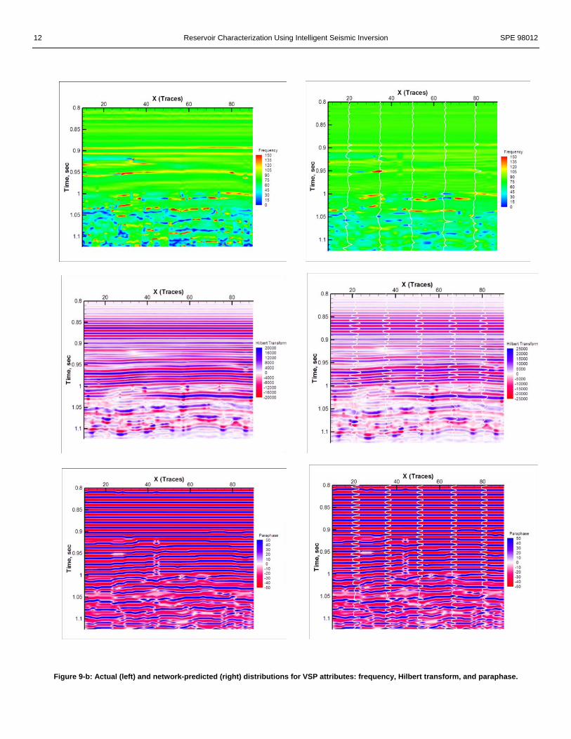
reliable training model by using all the available data. In this case, 90% of the total of 871 rows of data from five wells was used for training, while 10% was used for testing during training. Two types of logs: gamma ray and neutron porosity were selected as target logs. Because of the large number of available attributes a Key Performance Indicator (KPI) study was carried out, to determine the most influential attributes24. As a result of this study each attribute had a coefficient between 0 and 1, which basically shows the influence of that attribute on the selected output (i.e. logs). The attributes (including the time) were ranked based on their KPI coefficients and the ones having a coefficient larger than 0.5 were used as inputs. Those rankings for gamma ray and neutron porosity are shown in Table 3. The best thirteen attributes for the gamma ray, and the best eight attributes for the neutron porosity had coefficients higher than 0.5, and they were used as the input attributes. Training results were analyzed for each well separately, and upon applying those models to the other traces on the seismic line, distributions of gamma ray logs and neutron porosity logs were produced. Results and Discussions Case 1. Table 4 shows the correlation statistics of the training models developed for this step of the study. Correlation coefficient, r, and r-squared values are included as accuracy indicators of the match. Results for pattern (overall), training, calibration, and verification sets are included. Figure 8 shows the results of the training as actual vs. network-predicted plots for training, calibration, and verification sets of seven attributes. Each set of data is shown with a different symbol and color. Statistical and visual results indicate that reliable models have been developed. These models have been applied to the whole line (i.e. other traces of the synthetic model). The seismic attribute distributions have been re-produced. They have been re-plotted to be able to compare with the actual distributions. Figure 9-a shows the comparison plots for three attributes: amplitude, average energy, and envelope; and Figure 9-b shows the plots for three other attributes: frequency, Hilbert transform, and paraphase, which are obtained after applying the models for these attributes to the entire line. These plots also include the actual log lines of each attribute at traces 20, 35, 50, 65, and, 80, which makes it easier to assess the quality of the produced distributions. For the second step, where the density has been predicted; actual vs. network plot of the training model is shown in Figure 10-a. Although the network seemed to be successful in most parts, it has missed some points in the middle-valued region which was assumed to belong to Class 2: 2.3 g/cc. In order to overcome this problem, it has been decided to introduce another class to our model. Class 4 was assigned to density values around 2.09 g/cc (Figure 10-b). That has helped the network to be successful in that region (Figure 10-b), and this network model was chosen to be used in further studies. The correlation statistics of this model are shown in Table 5 together with the results for the velocity log. Actual VSP attributes were applied to this model, and density has been predicted along the seismic line with a correlation coefficient of 0.82. This has been repeated with the predicted VSP attributes coming from the first correlation step. The density has again been predicted through the seismic line with a


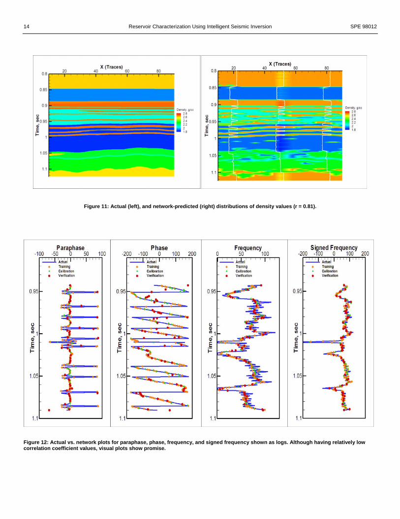
correlation coefficient value of 0.81. Figure 11 shows the final actual vs. network-predicted density distributions. It is seen that, the lithological units as well as the sand channels have been successfully predicted by the neural network. With this final result, the goal of predicting density log through the two-step intelligent seismic inversion methodology has been accomplished. The same procedure has also been applied to velocity and acoustic impedance. Case 2. As in the synthetic case, surface seismic – VSP correlation models have been developed, by using time and eleven surface seismic attributes to predict the single VSP attribute. The attributes used in this study were the ones which have been generated from the Kingdom Suite as the other attributes can be derived by using those ones. Table 6 shows the correlation statistics for these models for each attribute. Results for pattern, training, calibration, and verification sets are included. Verification results for phase, paraphase, frequency, and signed frequency seemed to be low. However, when plotted it seemed that they were not as bad as their correlation coefficients would suggest. Their actual vs. network graphs are shown in Figure 12. Actual vs. network plots for other attributes are shown in Figure 13. These models were then applied to other traces on the seismic line, with the available surface seismic data. VSP distributions were produced through the entire seismic line. In the log prediction stage, gamma ray and neutron porosity were selected as the target logs. The results for these two types of logs are presented below separately. Gamma Ray: Correlation statistics are shown in Table 7 for pattern, training, and testing sets, respectively. Results are showing both overall statistics, and separate well statistics. Graphs that show actual and network-predicted log lines are shown in Figure 14 for all wells. Figure 15 shows the predicted gamma ray distribution of the seismic line using these models. Actual log lines of five wells are also shown in the plot which may give a better perspective of comparisons. Neutron Porosity: Neutron porosity logs were available in only two wells; well-1 and well-2. Thus, these two wells were used in training. Correlation statistics of these models are shown in Table 8. Figure 16 shows the actual and network-predicted logs for two wells. Predicted distribution of neutron porosity is shown in Figure 17.

Conclusions In this study, a novel approach to the seismic inversion problem is introduced. A two-scale-step, intelligent seismic inversion methodology is successfully implemented on a synthetic model, and real data of the Buffalo Valley Field, New Mexico. The main conclusions of this study can be summarized as follows: 1) Even being in a complex and non-linear manner, it was shown that a relationship does exist between various seismic attributes and reservoir properties. Such a relationship can be extracted by using artificial neural networks, one of the major soft computing tools. Generalized regression neural network (GRNN), which is a useful algorithm for approximating continuous functions, was applied successfully in this study.

2) Benefits of using a synthetic seismic model were clearly seen in developing the appropriate methodology by identifying the most appropriate neural network algorithm and testing to use other tools. The synthetic model not only made it easy to be familiar with the type of data that is dealt with, but also provided the opportunity of comparing results for the whole seismic section. Although it was not applicable for the field study, the synthetic model was used for a classification (lithology identification) approach. 3) Although there are several examples of using artificial neural networks to correlate seismic attributes to reservoir properties, or well logs, this study is first of its kind simply because of integrating three types and scales of data (surface seismic, VSP, and well logs). 4) To determine the data that should be used for training, model visualization can be helpful. It was seen in the first correlation step of the synthetic model study that; including diverse geological characteristics in the training set can increase the prediction abilities of the neural network models. Acknowledgements This research was supported by a grant from the U.S. Department of Energy (DE-FC26-03NT41629). Authors would like to express their appreciation and gratitude to the project manager Mr. Thomas Mroz, for his help throughout the life of this project. Seismic and VSP data of the Buffalo Valley Field, used in this study were provided courtesy of WesternGeco. Authors also would like to acknowledge Janaina Pereira, for her help in digitizing well logs for the field study. Nomenclature C = City block distance V = Interval velocity D = Euclidian distance VR = Vertical resolution f = Dominant frequency W = Weight of a link I = Input of a neuron Y = Dependent variable i, j = Random numbers X = Independent variable n = No. of sample observations σ = Smoothing factor References

1. Nikravesh. M. and Aminzadeh, F.: ‘Past, present and future intelligent reservoir characterization trends’, Journal of Petroleum Science and Engineering, Vol. 31, pp.67-79, 2001.

2. Mohaghegh, S.D., Richardson, M., Ameri, S.: ‘Virtual Magnetic Imaging Logs: Generation of Synthetic MRI Logs from Conventional Well Logs’, paper SPE 51075, 1998 SPE Eastern Regional Meeting Proceedings, Nov. 9-11, Pittsburgh, Pennsylvania.

3. Mohaghegh, S.D., Goddard, C., Popa, A., Ameri, S., and Bhuiyan, M.: ‘Reservoir Characterization through Synthetic Logs’, paper SPE 65675, 2000 SPE Eastern Regional Meeting Proceedings, Oct. 17-19, Morgantown, West Virginia.

4. Rolon, L.: ‘Developing Intelligent Synthetic Logs: Application to Upper Devonian Units in PA’, M.Sc. thesis, West Virginia University, Morgantown, West Virginia, 2004.

5. Mohaghegh, S.D., Arefi, R., Ameri, S., and Rose, D.: ‘Design and Development of an Artificial Neural Network for Estimation of Formation Permeability’, SPE 28237, 1994 SPE Petroleum Computer Conference Proceedings, Jul. 31 - Aug. 3, Dallas, Texas.


6. Arpat, G.B., Gumrah, F., Yeten, B.: ‘The neighborhood approach to prediction of permeability from wireline logs and limited core plug analysis data using backpropagation artificial neural networks’, Journal of Petroleum Science and Engineering, Vol. 20, pp.1-8, 1998.

7. Weiss, W.W., Balch, R.S., Stubbs, B.S.: ‘How Artificial Intelligence Methods Can Forecast Oil Production’, paper SPE 75143, 2002 SPE/DOE Improved Oil Recovery Symposium Proceedings, April 13-17, Tulsa, Oklahoma.

8. Hampson, D.P., Schuelke, J.S., and J.A. Quirein: ‘Use of multiattribute transforms to predict log properties from seismic data’, Geophysics, Vol. 66, No. 1, pp. 220-236, 2001.

9. Leiphart, D.J., Hart, B.S.: ‘Comparison of linear regression and a probabilistic neural network to predict porosity from 3D seismic attributes in Lower Brushy Canyon channeled sandstones, southeast New Mexico’, Geophysics, Vol. 66, No. 5, pp. 1349-1358, 2001

10. Balch, R.S., Stubbs, B.S., Weiss, W.W., Wo, S.: ‘Using Artificial Intelligence to Correlate Multiple Seismic Attributes to Reservoir Properties’, paper SPE 56733, 1999 SPE Annual Technical Conference and Exhibition Proceedings, Oct. 3-6, Houston, Texas.

11. Chawathe, A., Ouenes, A., Weiss, W.W.: ‘Interwell property mapping using crosswell seismic attributes’, paper SPE 38747, 1997 SPE Annual Technical Conference and Exhibition Proceedings, Oct. 5-8, San Antonio, Texas.

12. Soto B. R., and Holditch, S.A.: ‘Development of reservoir characterization models using core, well log, and 3D seismic data and intelligent software’, paper SPE 57457, 1999 SPE Eastern Regional Conference and Exhibition Proceedings, Oct. 21-22, Charleston, West Virginia.

13. Reeves, S., Mohaghegh, S.D., Fairborn, J., and Luca, G.: ‘Feasibility Assessment of a New Approach for Integrating Multi-Scale Data for High-Resolution Reservoir Characterization’, paper SPE 77759, 2002 SPE Annual Technical Conference and Exhibition Proceedings, Sep. 29 - Oct. 2, San Antonio, Texas.

14. Gadallah, M.R.: Reservoir Seismology: Geophysics in Non-technical Language, PennWell Books, Tulsa, Oklahoma, 1994.

15. Taner, M.T.: ‘Seismic Attributes’, CSEG Recorder, pp. 48-56, September, 2001.

16. Kingdom Suite software tutorial, Seismic Micro-Technology, Inc., Houston, Texas.

17. Fausett, L.: Fundamentals of Neural Networks: Architectures, Algorithms, and Applications, Prentice-Hall, Englewood Cliffs, New Jersey, 1994.

18. Mohaghegh, S.D.: ‘Virtual Intelligence Applications in Petroleum Engineering - Part 1: Artificial Neural Networks.’ Journal of Petroleum Technology, Distinguished Author Series September 2000, pp 64-73.

19. Huang, Z., Williamson, M.A.: ‘Geological pattern recognition and modeling with a General Regression Neural Network’, Canadian Journal of Exploration Geophysics, Vol. 30, No. 1, pp. 60-66, 1994.

20. Luca, G.: ‘Towards High Resolution Reservoir Characterization’, M.Sc. Thesis, West Virginia University, Morgantown, West Virginia, 2001.

21. Specht, D.: ‘A General Regression Neural Network’, Vol. 2, No. 6, IEEE Transactions on Neural Networks, November, 1991.

22. NeuroShell 2, release 4.0 tutorial, Ward Systems Group, Inc., Frederick, Maryland, 1993-1998.

23. Sanchez, A.A.: ‘3D seismic interpretation and synthetic modeling of the Atoka and Morrow formations, in the Buffalo Valley Field (Delaware Basin, New Mexico, Chaves County) for reservoir characterization using neural networks’, M.Sc. thesis, West Virginia University, Morgantown, West Virginia, 2004.

24. KPI module of Intelligent Reservoir Characterization & Analysis, IRCA. http://www.intelligentsolutionsinc.com/irca.htm

Table 1: Density and interval velocity values for different types layers.

Lithology Density, g/cc Velocity, ft/s Sandstone Shale Limestone

2.3-2.6 1.9-2.1

2.5-2.71

12,500-16,000 9,000-11,000

14,000-17,000 Table 2: Properties of wavelets used to compute seismic responses.

Property 3D Seismic VSP Bandwidth, Hz Dominant Frequency, Hz Dominant Period, sec Interval Velocity, ft/sec Tuning Thickness, ft

11-95 45

0.022 15,000-16,000

83-88

20-110 65

0.0154 15,000-16,000

57-61 Table 3: Results of the Key Permormance Indicators for gamma ray and neutron porosity. Shaded ones were used as inputs.

Rank Gamma Ray Neutron Porosity 1 Peak-to-Trough Amp Weighted Phase 2 Smoothed Envelope Time 3 Finite Difference Peak-to-Trough 4 Average Frequency Instant Energy 5 Instant Energy Smoothed Envelope 6 Envelope Envelope 7 Time Amplitude 8 Amp Weighted Phase HF Inversion 9 Amplitude Finite Difference

10 Phase Average Energy 11 Hilbert Average Frequency 12 Smoothed Inversion Paraphase 13 HF Inversion Hilbert 14 1st D Amp Smoothed Inversion 15 Average Energy Decay Rate 16 Inst. Accel Phase 17 Inst. Q Fac Signed Freq 18 Decay Rate Frequency 19 2nd D Amp 1st D Amp 20 Res Env Inst Res Env 21 Frequency Inst Abs Amp 22 Inst Abs Amp Inst. Q Fac 23 Inst Res Env 1st D Env 24 1st D Env Res Env 25 Inst Power Inst. Accel 26 Signed Freq 2nd D Amp 27 Paraphase 2nd D Env 28 2nd D Env Inst Power

Table 4: Correlation statistics for seven VSP attributes, for the first correlation step of the synthetic model study.

Amplitude A. Energy Envelope Frequency r2 r r2 r r2 r r2 r

Pattern 1.00 1.00 0.83 0.91 0.97 0.98 0.76 0.87 Training 1.00 1.00 0.84 0.92 0.98 0.99 0.76 0.87 Calibration 1.00 1.00 0.79 0.89 0.90 0.95 0.81 0.90 Verification 1.00 1.00 0.75 0.86 0.92 0.95 0.73 0.86

Hilbert Trans. Paraphase Phase

r2 r r2 r r2 r Pattern 0.92 0.96 0.88 0.94 0.93 0.96 Training 0.93 0.96 0.89 0.94 0.97 0.99 Calibration 0.90 0.95 0.85 0.92 1.00 1.00 Verification 0.96 0.98 0.85 0.92 0.52 0.72


Table 5: Correlation statistics for density and velocity, for the second correlation step of the synthetic model study.

Density Aco. Velocity r2 r r2 r

Pattern 0.82 0.91 0.90 0.95 Training 0.94 0.97 0.93 0.96 Calibration 0.54 0.73 0.97 0.99 Verification 0.54 0.73 0.49 0.70

Table 6: Correlation statistics for eleven VSP attributes, for the first correlation step of the real case study.

Amplitude A. Energy Envelope Frequency r2 r r2 r r2 r r2 r

Pattern 0.97 0.98 0.96 0.98 0.98 0.99 0.34 0.58 Training 1.00 1.00 0.98 0.99 0.98 0.99 0.92 0.96 Calibration 0.91 0.95 0.98 0.99 0.98 0.99 0.83 0.91 Verification 0.90 0.95 0.85 0.92 0.85 0.92 0.21 0.46

Hilbert Trans. Paraphase Phase

r2 r r2 r r2 r Pattern 0.98 0.99 0.79 0.89 0.64 0.80 Training 0.98 0.99 0.98 0.89 0.96 0.98 Calibration 0.98 0.99 0.90 0.95 0.74 0.86 Verification 0.92 0.96 0.29 0.54 0.41 0.64

Finite Difference

Peak-to-Trough

Signed Frequency

Inversion

r2 r r2 r r2 r r2 r Pattern 0.92 0.96 0.93 0.96 0.46 0.96 0.98 0.99 Training 0.98 0.99 0.98 0.99 0.98 0.99 0.98 0.99 Calibration 0.98 0.99 0.90 0.95 0.86 0.93 0.98 0.99 Verification 0.83 0.91 0.79 0.89 0.09 0.30 0.98 0.99 Table 7: Correlation statistics for the pattern, training, and calibration sets of the training model for gamma ray log prediction.

Pattern Training Calibration r2 r r2 r r2 r

All 0.77 0.88 0.79 0.89 0.60 0.77 Well-1 0.58 0.76 0.57 0.75 0.73 0.85 Well-2 0.75 0.86 0.76 0.87 0.67 0.82 Well-3 0.66 0.81 0.72 0.85 0.27 0.52 Well-4 0.76 0.90 0.77 0.88 0.27 0.52 Well-5 0.81 0.90 0.82 0.91 0.69 0.83 Table 8: Correlation statistics for the pattern, training, and calibration sets of the training model for neutron porosity log prediction.

Pattern Training Calibration r2 r r2 r r2 r

All 0.95 0.97 0.96 0.98 0.82 0.91 Well-1 0.95 0.98 0.97 0.98 0.77 0.88 Well-2 0.94 0.97 0.95 0.97 0.89 0.94

Figure 1: Modeling high-frequency logs from low-frequency seismic signals. Schematic view of seismic inversion process with the proposed correlation map. Two major steps of correlation: 1)Surface Seismic – VSP, 2) VSP – Well logs. (Top portion: taken from Hampson et al.2)

Figure 2: Schematic diagram of an artificial neuron or a processing element. (Taken from Mohaghegh18)

Figure 3: VSP amplitude response of the synthetic model.


Figure 4: Cross-sectional envelope distribution, which was used to determine special features that can be useful in the network training. Finally, traces 32 and 57 were decided upon to be used in training.

Figure 5: Network structures used for training. a) Data of traces 32 and 57 have been used, to predict a VSP attribute from time and surface seismic attributes. b) Data of Trace - 50 have been used, to predict one of the density classes from time and VSP attributes.

Figure 6: Density log of Trace - 50. First classification proposed: Three classes at density values 1.9, 2.3, and 2.65

Figure 7: Amplitude distribution of the seismic line. Red dashed lines are the five wells that the line is passing through. Well-1 is the well with the VSP survey.

b)

a)


Figure 8: Actual vs. network results for each attribute after training the network for surface seismic - VSP correlation. Results for training, calibration, and verification sets are included with different symbols.


Figure 9-a: Actual (left) and network-predicted (right) distributions for VSP attributes: amplitude, average energy, and envelope.


Figure 9-b: Actual (left) and network-predicted (right) distributions for VSP attributes: frequency, Hilbert transform, and paraphase.


Figure 10: Defining density classes, and the corresponding training results. a) Three classes (1.9, 2.3, 2.65). r = 0.82 for training set, b) Four classes (1.9, 2.09, 2.3, 2.65). r = 0.94 for training set.

a)

b)


Figure 11: Actual (left), and network-predicted (right) distributions of density values (r = 0.81).

Figure 12: Actual vs. network plots for paraphase, phase, frequency, and signed frequency shown as logs. Although having relatively low correlation coefficient values, visual plots show promise.


Figure 13: Actual vs. network plots for seven of the attributes, that had satisfactory correlation statistics. Training, calibration, and verification sets are included with different symbols and colors.


Figure 14: Actual and network-predicted gamma ray logs for wells 1, 2, 3, 4, and 5. Values for training, and calibration sets are included. VSP attributes were used as inputs.


Figure 15: Network-predicted gamma ray distribution through the seismic line of interest. Actual log lines are also shown for five wells on the line. VSP attributes were used as inputs.

Figure 16: Actual and network-predicted neutron porosity logs for wells 1, and 2. Values for training, and calibration sets are included. VSP attributes were used as inputs.


Figure 17: Network-predicted gamma ray distribution through the seismic line of interest. Actual log lines are also shown for two wells on the line. VSP attributes were used as inputs.

spe 98012 reservoir characterization using intelligent ... · 2 reservoir characterization using...

Documents