spe 144376 production analysis in unconventional
TRANSCRIPT

SPE 144376
Production Analysis in Unconventional Reservoirs — Diagnostics, Challenges, and Methodologies D. Ilk, DeGolyer and MacNaughton, C.D. Jenkins, DeGolyer and MacNaughton,T.A. Blasingame, Texas A&M University Copyright 2011, Society of Petroleum Engineers This paper was prepared for presentation at the SPE North American Unconventional Gas Conference and Exhibition held in The Woodlands, Texas, USA, 14–16 June 2011. This paper was selected for presentation by an SPE program committee following review of information contained in an abstract submitted by the author(s). Contents of the paper have not been reviewed by the Society of Petroleum Engineers and are subject to correction by the author(s). The material does not necessarily reflect any position of the Society of Petroleum Engineers, its officers, or members. Electronic reproduction, distribution, or storage of any part of this paper without the written consent of the Society of Petroleum Engineers is prohibited. Permission to reproduce in print is restricted to an abstract of not more than 300 words; illustrations may not be copied. The abstract must contain conspicuous acknowledgment of SPE copyright.
Abstract
The analysis of production data in unconventional reservoirs to determine well/reservoir properties, completion effectiveness, and estimate future production has become popular in recent years. However, production analysis in unconventional reservoirs is a challenging task because of the non-uniqueness associated with estimating well/reservoir properties. Various analysis methodologies exist in the literature, but no single methodology is robust enough to characterize the production data and forecast production. Therefore, from a conceptual standpoint, we believe that production analysis in unconventional reservoirs should not be a "single-method based" application. Instead, multiple analysis techniques combined with diagnostic tools have to be utilized, and challenges associated with the analysis have to be recognized.
This work attempts to provide a review of the existing production analysis and diagnostic techniques as well as to identify the challenges associated with production analysis in unconventional reservoirs. We present an extensive evaluation of the diagnostic tools for assessing data viability, checking data correlation along with flow regime identification. Based on diagnostics and analysis results, we demonstrate the use of forward modeling (simulation) to predict future performance of single/multiple well(s) for various production/completion and field development scenarios. Field examples from a wide range of unconventional reservoirs are used to describe the application of the methodology. Introduction
Unconventional reservoir systems such as tight gas sands, shale gas, tight/shale oil, and coalbed methane reservoirs have currently become a significant source of hydrocarbon production and offer remarkable potential for reserves growth and future production. Unconventional reservoir systems can be described as hydrocarbon accumulations which are difficult to be characterized and produced by conventional exploration and production technologies. Complex geological and petrophysical systems describe unconventional reservoirs in addition to heterogeneities at all scales similar to conventional reservoir systems. Because of the low to ultra-low permeability of these reservoir systems, well stimulation operations (e.g., single or multi-stage hydraulic fracturing, etc.) are required to establish production from the formations at commercial rates.
For a long time unconventional reservoirs have been thought too complicated to produce because of the complexity and very low permeability of these reservoir systems. However, recent advances in the technology at lower costs lead the way for the exploitation of these reservoir systems. In particular, production from the unconventional reservoirs such as tight gas sands, coalbed gas, shale gas, and tight oil, has increased drastically in the recent years. According to the IEA (IEA 2009) proven reserves of unconventional gas have grown at a fast pace and now account for 4% of the worldwide total natural gas reserves. Production from unconventional gas reservoirs has become a major source of the United States natural gas supply and accounts for 47% of natural gas production (EIA 2009). Specifically, natural gas production from shale gas reservoirs is increasing rapidly and expected to account for 24% of US natural gas production in 2030 from 6% in 2008 (EIA 2010).
The advances in technology to produce and develop ultra-low permeability reservoirs such as shale gas reservoirs bring the difficulties and uncertainty associated with well performance. The uncertainty is mainly due to the lack of our fundamental understanding of the production mechanisms and behavior of these reservoirs. Currently a handful of diagnostic methods, which are based on linear/compound linear flow concepts exist to diagnose the flow behavior of this type of wells.

2 SPE 144376
The solutions based on the "linear flow" concept (Wattenbarger et al. 1998; El-Banbi and Wattenbarger 1998) are frequently used with the inclusion of effective fracture network length accounting for a single vertical fracture. Bello and Wattenbarger (2010) extend the previously mentioned linear flow solutions to account for the natural fracture network in shale gas reservoirs by proposing a linear dual porosity solution. Bello and Wattenbarger state that transient linear flow regime (drainage from matrix to fracture system) should generally be the case for field data in shale gas reservoirs. Consequently, slope of the straight line exhibited by the data, in the rate versus square root of time plot yields the matrix drainage area provided that the matrix permeability is known during transient linear flow regime. The deviations from linear flow can be attributed to skin factor effects. We note that establishing the linear flow trend could often be subjective and the conductivity of fractures might affect the production behavior.
Regardless of diagnostics, for horizontal wells completed with multiple fractures in ultra-low permeability reservoirs, we suggest that multiple-fractured horizontal well model should be used for analysis. The references on this particular well model in fact extend to late 1980s. van Kruysdijk and Dullaert (1989) provide an analytical solution based on "boundary-element method". van Kruysdijk and Dullaert show that at early time dominant flow is linear, perpendicular to the fracture face until pressure transients of the individual fractures begin to interfere leading to a compound linear flow regime at late times (linear flow is seen towards the collections of fractures during compound linear flow regime). Eventually, pseudoradial flow should occur, however we must note that the occurrence of pseudoradial flow regime should not be expected in ultra-low permeability shale gas reservoirs. Other analytical solutions for horizontal wells with multiple fractures include the works by Soliman, Hunt, and El Rabaa (1990), Larsen and Hegre (1991), Guo and Evans (1993), Larsen and Hegre (1994), Horne and Temeng (1995), Chen and Raghavan (1997), and Raghavan, Chen, and Agarwal (1997).
Ozkan et al. (2009) and Brown et al. (2009) present an analytical trilinear flow solution including dual porosity idealization to simulate the pressure transient and production behavior of horizontal wells with multiple fractures. The trilinear solution given by Ozkan et al. (2009) and Brown et al. (2009) is based on coupling of individual "outer reservoir, inner reservoir, and fracture" solutions using the pressure and flux continuity conditions on the interfaces between the regions. We note that dual porosity idealization is used to account for natural fracture network. Meyer et al. (2010) provide an approximate analytical solution for horizontal wells with multiple finite-conductivity transverse fractures. The solution by Meyer et al. is based on a trilinear flow solution (Lee and Brockenbrough 1986) and includes fracture interference.
Medeiros, Ozkan, and Kazemi (2006) present a semi-analytical approach to obtain pressure-transient solutions for heterogeneous systems — this approach gives the ability to model various kinds of well responses in many types of heterogeneous reservoirs including shale gas reservoirs. Amini and Valkó (2010) use a semi-analytical solution, namely the method of "distributed volumetric sources", to predict the performance of a horizontal well with multiple transverse fractures in a bounded reservoir. Amini and Valkó solution includes non-Darcy flow effect in fracture.
The use of only production data (i.e., rate-time data) to estimate future production has been an industry practice since the introduction of the Manual for the Oil and Gas Industry under the Revenue Act of 1918 by the United States Internal Revenue Service (1919). Lewis and Beal (1918) provides initial guidance on the extrapolation of future production of oil wells. Cutler (1924) presents a detailed review of the oil reserves estimation procedures in 1920's. Johnson and Bollens (1927) introduce the loss ratio and the loss ratio derivative definitions which lay the basis for the exponential and the hyperbolic rate decline relations. Arps (1945) presents the derivation of empirical exponential and hyperbolic rate decline relations, which are still the widely used relations for production extrapolations of oil and gas wells, and can be assumed as valid for a variety of producing conditions for practical purposes. We note that the exponential and hyperbolic relations are only applicable for the boundary-dominated flow regime and the improper use of Arps' equations can yield inconsistent results and erroneous future production values. The common industry practice for production extrapolation in unconventional reservoirs is to use the hyperbolic relation, but as mentioned before the hyperbolic relation is strictly applicable during boundary-dominated flow. Application of the hyperbolic relation to transient flow often results in significant overestimation of future production. For reference the hyperbolic rate decline and cumulative production relations are given as:
bi
i
tbD
qtq
/1)1()(
+= ............................................................................................................................................................. (1)
])1(1[ )1(
)( )/1(1 bi
i
ip tbD
DbqtG −+−−
= .............................................................................................................................. (2)

SPE 144376 3
According to Arps' definition, the value of the b-parameter is constant and should lie between 0 and 1. If the b-parameter value is higher than 1, the extrapolation of Eq. 2 to infinity yields infinite cumulative production. When hyperbolic rate decline relation is applied to rate-time data in unconventional reservoirs, we usually observe b-parameter values higher than 1 which might lead to overestimation of future production. To prevent overestimation of future production, production forecast with hyperbolic rate decline relation can be switched to exponential rate decline relation at a specified time (based on the knowledge of a constant percentage decline value). This procedure (or the so called "modified hyperbolic relation") is a practical way to constrain future production. However, rate-time data characteristics indicate that the nature of rate-time data is in fact not hyperbolic when the hyperbolic rate decline model parameters are computed continuously using data. In particular, the computed b-parameter data trend indicates that the value of b-parameter would not be constant throughout the producing life of the well.
The issues related to the use of "conventional" rate decline relations to estimate future production in "unconventional" reservoirs, have led us to focus on the character of the rate-time data. Our primary objective is to understand the characteristic behavior of rate-time data in unconventional reservoirs, and to develop appropriate rate decline relation(s) based on the characteristic behavior. For these purposes, we recall the original definitions of the "loss-ratio" and the "loss-ratio derivative", which were previously introduced by Johnson and Bollens (1927). These definitions are given as:
dttdqtq
D /)()(1
−≡ (Definition of the loss-ratio) ...................................................................................... (3)
⎥⎦
⎤⎢⎣
⎡−≡⎥⎦
⎤⎢⎣⎡≡
dttdqtq
dtd
Ddtdb
/)()(1 (Derivative of the loss-ratio) ..................................................................................... (4)
Continuous evaluation of Eqs. 3 and 4 requires numerical differentiation, which might be problematic if the data quality is poor. Usually the data quality is significantly affected by non-reservoir affects (e.g., well clean-up, liquid loading, etc.) and operational changes (e.g., choke changes, refracturing, etc.). Therefore, vigilant editing is warranted and redundant/erroneous data points have to be removed prior to differentiation. We use the derivative algorithm, proposed by Bourdet, Ayoub, and Pirard (1989) for numerical differentiation to provide desired smoothness on the derivatives. It is also worth to mention that the "loss-ratio" and "loss-ratio derivative" can be calculated alternatively using rate and cumulative production data. Using the rate-cumulative production data to calculate loss-ratio and loss-ratio derivative provides more resolution as rate-cumulative production data is smoother than rate-time data. The alternate formulations for the loss-ratio and loss-ratio derivative are given as:
dqdG
Dp−≡
1 (Definition of the loss-ratio) .......................................................................................................... (5)
⎥⎦⎤
⎢⎣⎡≡
DdGdqb
p
1 (Derivative of the loss-ratio) .......................................................................................................... (6)
Based on the loss-ratio and the derivative of the loss-ratio definitions, the D- and b-parameters are computed continuously and the character of the computed trends is evaluated. It is observed that the computed D-parameter trend exhibits power-law behavior (i.e., straight line on log-log scale) as a function of time and the computed b-parameter data trend is not constant contrary to the hyperbolic rate decline relation (Ilk et al. 2008, Mattar et al. 2008). Therefore, it can be stated that "power-law" behavior of the loss-ratio can be considered as a general characteristic of rate-time data in unconventional reservoirs, and we observe this behavior in almost all the cases in unconventional reservoirs (Ilk 2010). Power-law exponential rate-decline relation is derived from this observation (Ilk et al. 2008).
]ˆexp[ˆ)( tDtDqtq nii ∞−−= ................................................................................................................................................. (7)
Valko (2009) presents another form of Eq. 7 (namely the "stretched exponential function"), which is given as:
])/(exp[ˆ)( ni tqtq τ−= ........................................................................................................................................................ (8)
4 SPE 144376
Recent developments in well completion technology have transformed the unconventional reservoir systems into economically feasible reservoirs. However, the uncertainty associated with future production and non-uniqueness related with well/reservoir parameter estimation are the main issues in future development of these reservoirs. The primary goal of this study is to reduce the uncertainty and non-uniqueness to a certain extent by developing a systematic procedure, which makes use of physical models and rate-time relations along with data diagnostics, to properly characterize the flow behavior/well performance and extrapolate production of the wells in unconventional reservoirs into future. Production Data Diagnostics
We believe that one of the most important tasks in well performance evaluation of unconventional reservoirs is production data diagnostics. Integrating production data diagnostics with production analysis methodologies should reduce the uncertainty in determining reservoir characteristics, completion effectiveness, and future production to a considerable extent. In simple terms, production data diagnostics is crucial in verifying data consistency/viability and identifying flow regimes exhibited by the well production data. In addition, wells producing in a similar manner can be identified and confirmed using diagnostic methods before any analysis tasks are performed.
Ilk et al. (2010) present detailed review of production data diagnostics and analysis methodologies along with the challenges and pitfalls of production analysis in order to provide guidance towards best practices and best tools. In this work our main objective is to extend the scope of previous work to unconventional reservoirs. In particular, we attempt to distinguish characteristic features exhibited by data in order to develop a diagnostic understanding of the production sequence, and to develop a characteristic understanding of the reservoir model.
As mentioned earlier, production data diagnostics is mainly utilized for two purposes. First, measured data are reviewed to check for correlation between pressure and rate data. This is very important because data having no correlation will not provide any diagnostic value. Also, this way we can detect the features or events which should be filtered or discarded prior to analysis. Next, characteristic features, which are exhibited by production data, are identified with the use of diagnostic plots. Diagnostic plots help to identify flow regimes (e.g., bi-linear/linear flow, compound linear flow, etc.) and compare data to a well/reservoir model. Although the complexity of unconventional reservoirs prevents the establishment of a rigorous analytical solution (at present) to account for the actual well/reservoir model that is applicable for unconventional reservoirs, we can at least observe the characteristic behavior(s) of the wells producing in unconventional reservoirs using diagnostic plots. For example, plot of the computed D-parameter (see "loss-ratio" definition Johnson and Bollens (1927) and Arps (1945)) versus production time exhibits power-law behavior which can be translated into a rate-time relation known as the "power-law exponential" relation (Ilk et al. 2008). Once the characteristic features of well performance data are identified, we can make use of semi-analytical and/or numerical solutions for tuning to the data and estimating the flow efficiency, completion effectiveness, reservoir properties, and consequently future production. If we identify similarly producing wells from diagnostics, we can also group the wells accordingly and generate the characteristic performance trend for the selected wells producing in a particular field.
Challenges/Pitfalls: There are certain challenges/pitfalls that one may encounter when analyzing/interpreting production data from unconventional reservoirs. It is imperative that these issues need to be recognized, if not addressed. Failure to address these issues will almost certainly affect the outcome of production analysis from unconventional reservoirs in the form of analyzing artifacts (i.e., an artifact is a feature in the data which is not related to the reservoir behavior, but may be interpreted as reservoir behavior if not properly recognized). These common challenges/pitfalls can be listed in Table 1 as:
SPE 144376 5
Table 1 — Common challenges/pitfalls in production data analysis in unconventional reservoirs.
Issue
Influence/Severity
Pressure: — No pressure measurement(s) — Incorrect initial pressure estimate — Poor ptf → pwf conversion (models) — Liquid loading — effect on ptf → pwf conversion — Incorrect location of pressure measurement (at surface) — Drift/failure of a pressure gauge(s)
High High High to Very High Moderate to High High to Very High Very High
Flowrate: — Errors in rate allocations — Errors in metering (poor calibrations, multiphase flow, failures, etc.) — Effect of water rates on the ptf → pwf conversion —Total "single-phase" equivalent rate calculation (for condensate)
Moderate to High Moderate to High Very High (early) High
Well Completion: — Zone changes — new/old perforations — Changes in the wellbore tubulars — Changes in surface equipment — Offset fracture interference — Sand/shale production
High to Very High High Moderate to High Low to Very High High
General: — Pressure-dependent reservoir properties — Oil properties (Bo, Rso, μ o, co, etc.) — Gas properties (γg, T, z (or Bg), μg, cg, etc.) — Poor time-pressure-rate synchronization (in time) — Poor time-pressure-rate correlation (data events are uncorrelated) — Multiphase flow in the wellbore (flow slugging or loading) — Multiphase flow in the reservoir/fracture system (flow reduction)
High Moderate to High Low to Very High Very High Very High Moderate Moderate to High
Diagnostic Plots: The underlying idea of using diagnostic plots is to find out if certain feature(s) exist from a given data profile. If a certain character exists from the data profile then we can attribute this to the relevant reservoir signal. Also from a qualitative point of view, a diagnostic plot should highlight if there is something wrong with the data and identify the causes of (mis)behaviors from the data plot. We prefer to use diagnostic plots along these lines that is we initially seek to verify the correlation between a flowrate and flowing pressure data set, and if we establish that data can be analyzed then we proceed to reservoir diagnostics. We can either perform diagnostics on a single well to identify a certain character or perform diagnostics on multiple wells to compare flow efficiencies, completion effectiveness, and reservoir signal. If the wells are producing in the same area, diagnostics can significantly help in distinguishing the stimulation effectiveness so that the better performing wells are identified and the issues for poorly performing wells can be addressed.
In this work we propose to use the following diagnostic plots (Table 2) for our purposes:
These plots have been proposed historically as diagnostic plots for production data from theory and practice, and we believe that these plots would contribute to our better understanding of well performance.
We make use of production data of 9 wells, which are producing in the same area in a shale gas reservoir, to illustrate the use of diagnostic plots. We present the "history and data correlation" plots for each well separately (Figs. 1.x - 9.x) and "reservoir diagnostics" plots for all wells plotted in one plot. Again, our main objective is to review production data and establish the data correlation for each well individually using the history and data correlation plots and compare the performances of all wells using the reservoir diagnostics plots.
As mentioned earlier Figs 1.x - 9.x present the history and data correlation plots for each well. Although there are some minor issues with each well, these issues do not prevent the data to be analyzed since for most of the cases pressure and rate data seem to be correlated. We believe that these issues are more or less related to the challenges/pitfalls listed before. For example, the erratic behavior of pressure and flowrate data almost after 350 days on Fig. 6a and Fig. 6b is a result of offset fracture interference. For analysis purposes these data can be omitted prior to analysis.

6 SPE 144376
Table 2 — Proposed diagnostic plots for production data diagnostics.
Proposed Diagnostic Plots
History and Data Correlation: — log(qg) and pwf vs. t — log(qg) and pcf and ptf vs. t — log(qg) and Gp vs. t — qg vs. Gp — qg vs. pwf
Reservoir Diagnostics: — log(qg/Δp) vs. log(t) — log(qg/Δp) vs. log(G /q) p— log(qg/Δp) vs. log(t0.5)
— (qg/Δp) vs. Gp
— log(Gp/Δp) vs. log(t) — log(Gp/Δp) vs. log(Gp/q) — log(Gp/Δp) vs. log(t0.5)
— (Δp/qg) vs. t — (Δp/qg) vs. Gp/q —(Δp/qg) vs. t0.5
— log(D) vs. log(t) — log(b) vs. log(t) — log(βq-cp) vs. log(t)
For well performance considerations, we first plot the productivity index versus various time functions (i.e., production time, material balance time, and square root of production time). Plotting the productivity index versus various time functions provide more resolution, but one needs to be careful since the use of specific time functions implicitly imposes the solution on the plot — for example, straight line trends can be observed as evidence of linear flow in square root of time plots although linear flow is not existent. Nevertheless, Figs 10a. - 10c indicate that production performance of all the wells is similar leading us to the conclusion that completion effectiveness for these wells is relatively the same.
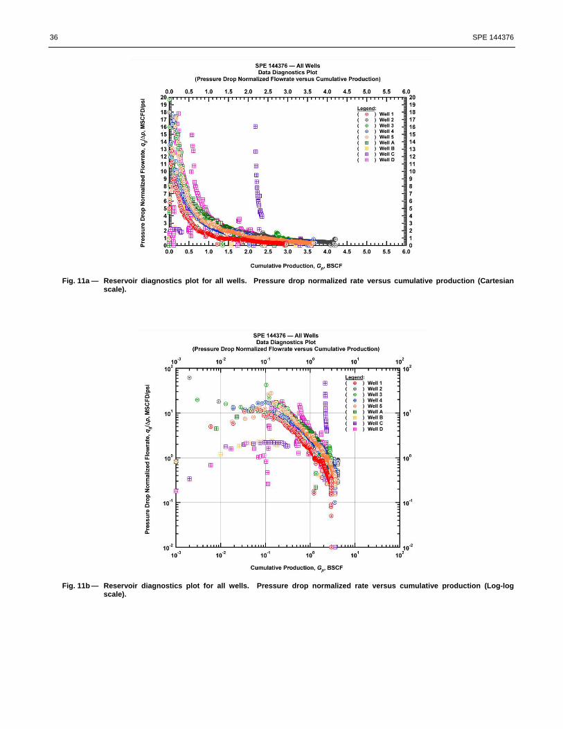
We present the productivity index versus cumulative production (flowing material balance type plot) in Fig. 11a (Cartesian scale) and Fig 11b (Log-log scale). Our observations are similar to the observations in Fig. 10.x. In addition we detect that Well 1 is performing worse than the other wells — this is most likely due to a completion issue. And, we observe in Fig. 11b that productivity index of these wells are decreasing higher than expected. The severe loss in the productivity over time might be due to factors causing additional pressure drop over time such as pressure-dependent permeability and fracture conductivity, proppant embedment, sand/shale production, non-Darcy skin, etc.
Figs. 12a - 12c present the productivity of these wells in terms of pressure drop normalized cumulative production. The faster stabilization of the pressure drop normalized cumulative production trends indicates decreasing productivity as well. In fact, plotting the pressure drop normalized cumulative production might be considered as a zero order attempt to approximate the cumulative production function if the well is produced at a constant bottomhole pressure. Although this is a very rough approximation, it can still give the analyst an idea about comparing the performances of the wells under consideration.
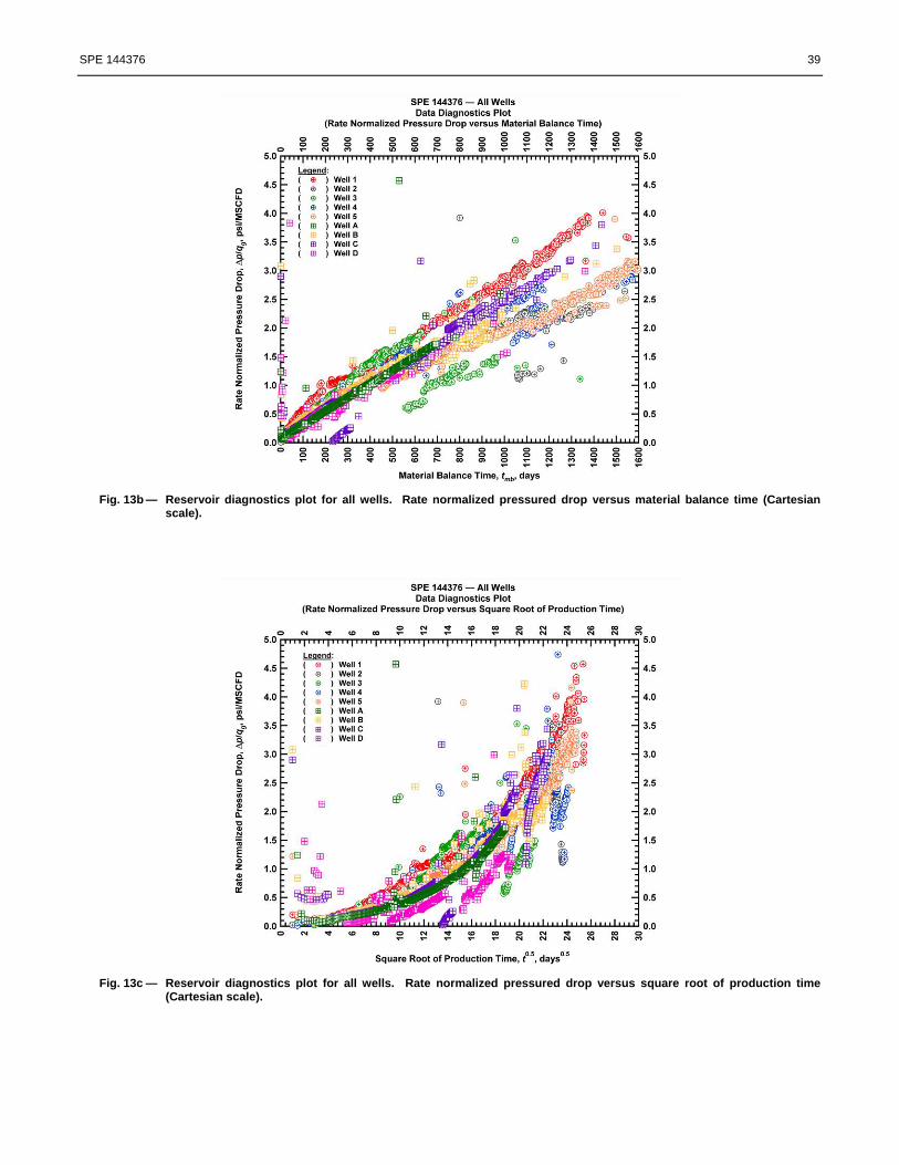
We plot the reciprocal of the productivity index versus various time functions in Figs. 13a - 13c. These plots are basically the reciprocal of Figs. 10a - 10c except that they are plotted in Cartesian scale. This view of the data functions may help to understand which well is exhibiting more pressure drop over time causing higher productivity loss. It can be derived from Figs. 13a - 13c that Well 1 exhibits more productivity loss over time. It is also observed almost all the wells have the same producing character. Again, the differences are attributed to well completion efficiencies. It is worth to note that the use of material balance time corrects the rate normalized pressure drop function for Well C and Well D (see Fig. 13b). Again according to Fig. 13b Well C and Well D are the wells showing more productivity loss over time.
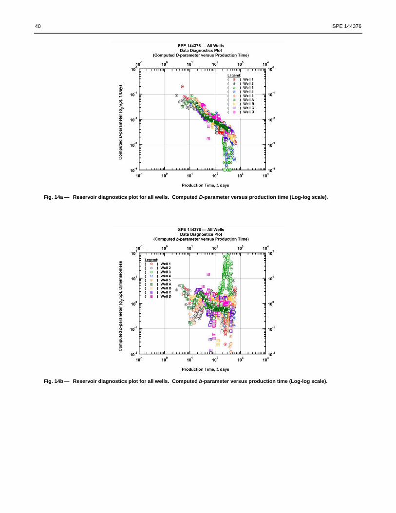
Finally, in Figs. 14a - 14c we present the characteristic behavior of these wells in terms of loss-ratio and βq-cp-derivative formulations. For our purposes instead of using only the rate data, we prefer to use pressure drop normalized rate data to account for the pressure variations throughout the production sequence. The definitions for the loss-ratio and its derivative were given earlier in Eqs. 3 and 4 (or Eqs. 5 and 6). On the other hand, βq-cp-derivative (Ilk et al. 2010) is formulated as:

SPE 144376 7
dttptqd
tptqt
tdtptqdtcpq
))()(()(/)(]ln[
)](/)(ln[)(,Δ
Δ−=
Δ−=β ................................................................................................. (9)
The advantage of the βq-cp-derivative is that βq-cp-derivative is dimensionless, which is in fact a very convenient to compare performance of the wells under investigation. Fig. 14a presents the computed D-parameter of the wells from pressure drop normalized rate data function. As seen, this result is in agreement with Ilk et al.'s observations (2008) on the characteristic behavior of rate data in unconventional reservoirs. The computed D-parameter data on Fig. 14a can be modeled with a single power-law function which would eventually yield the power-law exponential function to account for the characteristic performance of these wells. However, it is important to note that the obtained function for the characteristic behavior of the data is cast in terms of pressure drop normalized rate function.
Fig. 14b presents the computed b-parameter versus time plot. Since data is differentiated twice for continuous evaluation of b-parameter data, too much scatter is observed on Fig. 14b. However, this could still yield a range for the b-parameter if hyperbolic relation is used. For these cases the b-parameter range from 0.6 to 1.3 as observed from Fig. 14b. Again we note that the b-parameter is calculated using the pressure drop normalized rate function. In Fig. 14c the computed βq-cp-derivative function data is plotted against production time. From this plot it is possible to conclude that almost all wells are exhibiting similar production behavior as the computed βq-cp-derivative function data for each well follow relatively the same trend. Production Data Analysis — Characteristic Performance
Based on production data diagnostics, it is observed that these wells have very similar production behavior. Although we can go ahead and analyze each well individually to obtain well/reservoir properties and production forecast, we prefer to pick only two wells, which can be considered as representative of all the wells, and analyze only two wells to establish the characteristic performance with respect to the specific area in this shale gas reservoir of interest. Using diagnostics, we have already established that completion/stimulation effectiveness of these wells are similar (geology is more or less out of question as these wells are producing in the same area), and therefore the remaining task is to quantify the well/reservoir and completion parameters using production data analysis for production optimization and production forecast.
All these wells are horizontal wells with multiple transverse fractures. Therefore, we first attempt to use the semi-analytical solution developed by Larsen and Hegre (1994). This semi-analytical solution assumes horizontal well configuration intersected by vertical fractures, homogeneous or dual-porosity reservoir, and infinite or finite conductivity fractures. We note that since this is a semi-analytical solution, if non-linearities (such as pressure-dependent properties, non-Darcy skin, etc.) are present then this solution would not be able to handle all the issues. Nevertheless, it can serve as a good starting point to establish initial values for permeability, fracture half-length, fracture conductivity.
We pick the Well 5 and Well D for analysis purposes. Initially we use the semi-analytical solution to match the data with the solution; however our efforts are not successful for history matching purposes due to severe productivity loss exhibited by these wells. It can be stated that the productivity loss introduce non-linearities into the system. And thus the production data can only be analyzed with accounting for the non-linearities. At this point we attempt to use numerical solution which accounts for the severe productivity loss via pressure-dependent rock properties (i.e., k(p) and φ(p)). We have obtained very good matches of the data with the numerical solution when pressure-dependent rock properties are included in the solution. Fig. 15 and Fig. 16 present the history matches of the data with the numerical solution. Particularly, it is very interesting to observe the excellent match of the pressure buildup data with the model in Fig. 16. Although, these matches can be very satisfactory, we advise extreme caution with the use of numerical solution with pressure-dependent rock properties. We strongly suggest starting with the simpler semi-analytical solution, establishing the initial values for the well/reservoir properties and then proceeding to numerical solution for analysis and modeling purposes. For reference, we summarize the model-based analysis results in Table 3 below:
Table 3 — Model-based analysis results and model parameters for characteristic performance model.
Effective permeability, k = 530 nd Fracture half-length, xf = 350 ft Fracture conductivity, Fc = Infinite Number of fractures, nf = 48 Horizontal well length, Lw = 4786 ft Skin factor, s = 0.01 (dimensionless) k(p) and φ(p) = included

8 SPE 144376
Production Forecast
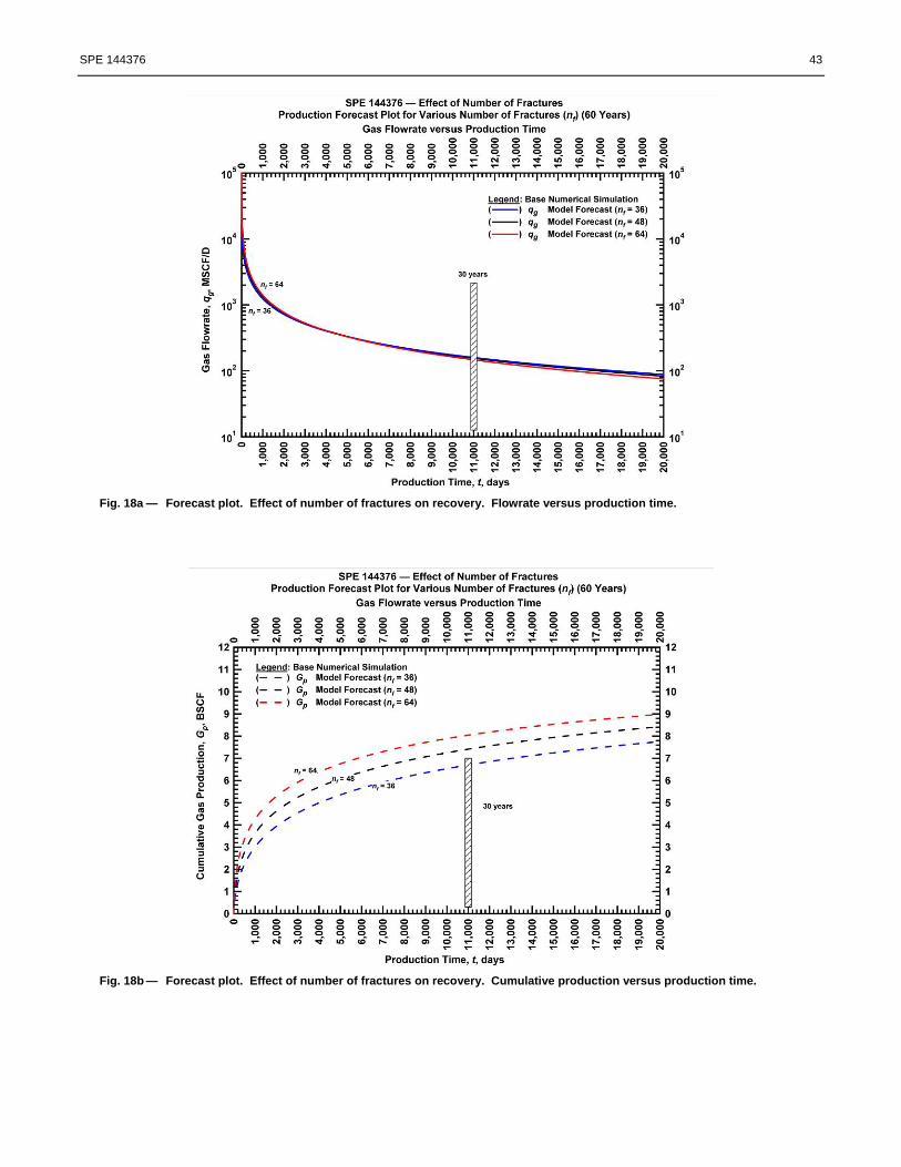
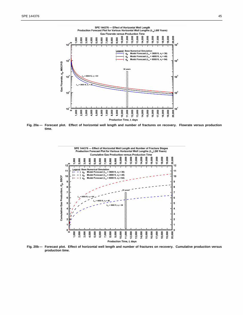
In this section we concentrate our efforts on production optimization and production forecast. First, we forecast production with the obtained characteristic performance from production data diagnostics and analysis of the wells producing in this specific area. Using the model parameters from Table 3 we generate a constant pressure simulation scenario (constant pressure is equal to the line pressure, pwf = 1500 psia) and estimate the cumulative production value at 30 years. The results of this simulation run (i.e., generated flowrate and cumulative production) are presented in Fig. 17. In this field characteristic performance indicates a cumulative production of almost 7.4 BSCF for a single well in this field. Next, we turn our attention to production optimization. We run sensitivities on the following parameters and investigate the effect on the ultimate recovery (at 30 years). The parameters, we run sensitivities on, include:
● Number of fractures. ● Horizontal well length. ● Number of fractures and horizontal well length. ● Drainage area.
The results of the sensitivity study are plotted on Fig. 18 - Fig. 21. From this study it is clear that with improved completion, the recovery increases. It is also worth to mention that there is 25% difference in recovery in 80 acres and 320 acres spacing cases. Summary and Conclusions
Summary: In this work we attempt to demonstrate a workflow to evaluate well performance data in unconventional reservoirs. The workflow has three major components: production data diagnostics, production data analyis, and production forecast. There are no strict rules for which methodologies to use for each component of the workflow, but we strongly suggest that the analyst has to pay particular attention for each component, especially for production data diagnostics. The workflow can be summarized as a stepwide procedure as follows:
1. Diagnosis of production data ■ Data correlation check ■ Data review/editing and filtering ■ Reservoir diagnostics/flow regime identification
2. Analysis of production data based on production data diagnostics ■ Simple analytical solution(s) (e.g., bilinear/linear flow solutions, etc.) ■ Semi-analytical solution(s) (horizontal well with multiple fractures solution(s)) ■ Numerical solution to account for non-linearities/decreasing well productivity (e.g., pressure-dependent properties,
decreasing fracture-conductivity, non-Darcy skin factor, etc.)
3. Production forecast based on reservoir model ■ Production extrapolation using the well/reservoir model ■ Comparison of well/reservoir model forecast with rate-time decline relations ■ Production optimization/sensitivity analysis using the well/reservoir model
In this work we apply the described workflow to a number of wells producing in the same field in a shale gas reservoir. Based on production data diagnostics we are able to produce a characteristic performance model which can be representative for these wells, and consequently we generate a characteristic production forecast for this field.
Conclusions: We state the following conclusions based on this work:
1. Production data diagnostics is crucial in the characteristic evaluation and analysis of production data. Also diagnostic plots assist in assessing the quality and character of the production data. Using production data diagnostics certain features/character exhibited by production data can be identified. The use of diagnostic plots for the evaluation of a number of wells, which are producing in the same area, can help to establish completion/stimulation effectiveness of these wells.
2. Model-based analysis should be considered as the most important task in production analysis rather than the use of simplified solutions. Model-based analysis should also be a product of a systematic diagnostic process. In this work we show that a characteristic performance model for the wells considered in this study can constructed using model-based analysis.

SPE 144376 9
3. It is not possible to analyze well performance data exhibiting severe productivity loss with analytical/semi-analytical solutions. In these cases, it is suggested that non-linearities should be taken into account using numerical solution. These non-linearities include but not limited to pressure-dependent rock/fluid properties, non-Darcy skin, proppant embedment, pressure-dependent fracture conductivity. It is also suggested that for these cases it would be better to start off with a semi-analytical/analytical solution and establish initial parameters then proceed to numerical simulation.
4. Sensitivity analysis for various parameters such as number of fractures, horizontal well length, and drainage area (based on the characteristic performance model for this field) indicates that better completion/stimulation would yield higher recovery for a single well in this field. Obviously this study does not consider any economic analysis on the cost and revenue; therefore we leave this evaluation to the reader's consideration.
Nomenclature
Variables:
A = Drainage area, ft2 b = Arps' decline exponent, dimensionless D = Reciprocal of loss ratio, D-1 Di = Initial decline constant for exponential and hyperbolic rate relation, D-1 D∞ = Power-law exponential model parameter, D-1
iD̂ = Power-law exponential model parameter, D-1 EUR = Estimate of ultimate recovery, BSCF Fc = Fracture conductivity, md-ft Gp = Cumulative gas production, MSCF or BSCF Gp,max = Maximum gas production (at a specified time limit), MSCF or BSCF k = Formation permeability, md Lw = Horizontal well length, ft n = Time exponent for power-law exponential model, dimensionless nf = Number of fractures, dimensionless pi = Initial reservoir pressure, psia pcf = Casing (surface) pressure, psig ptf = Tubing (surface) pressure, psig pwf = Flowing bottomhole pressure, psia q = Production rate, MSCF/D or STB/D qi = Initial production rate for exponential and hyperbolic relations, MSCF/D or STB/D
iq̂ = Power-law exponential model parameter, MSCF/D or STB/D xf = Fracture half-length, ft s = Skin factor, dimensionless t = Production time, days
Greek Symbols:
βq,cp = Beta-derivative function (constant-pressure), dimensionless φ = Porosity, fraction μ = Viscosity, cp τ = Dummy variable, dimensionless

10 SPE 144376
References
Amini, S. and Valkó, P.P. 2010. Using Distributed Volumetric Sources to Predict Production from Multiple-Fractured Horizontal Wells Under Non-Darcy-Flow Conditions. SPEJ 15 (1): 105-115.
Arps, J.J. 1945. Analysis of Decline Curves. Trans. AIME 160: 228-247.
Bello, R.O., and Wattenbarger, R.A. 2010. Multi-stage Hydraulically Fractured Shale Gas Rate Transient Analysis. Paper SPE 126754 presented at the SPE North Africa Technical Conference and Exhibition, Cairo, Egypt, 14-17 February.
Bourdet, D., Ayoub, J.A., and Pirard, Y.M. 1989. Use of Pressure Derivative in Well-Test Interpretation. SPEFE 4 (2): 293-302.
Brown, M., Ozkan, E., Raghavan, R., and Kazemi, H. 2009. Practical Solutions for Pressure Transient Responses of Fractured Horizontal Wells in Unconventional Reservoirs. Paper SPE 125043 presented at the SPE Annual Technical Conference and Exhbition, New Orleans, LA, 04-07 October.
Chen, C.C. and Raghavan, R. 1997. A Multiply-Fractured Horizontal Well in a Rectangular Drainage Region. SPEJ 2 (4): 455-465.
Cutler, W.W. 1924. Estimation of Underground Oil Reserves by Oil-Well Production Curves. Bull. U.S. Bureau of Mines 228.
El-Banbi, A.H. and Wattenbarger, R.A. 1998. Analysis of Linear Flow in Gas Flow Production. Paper SPE 39972 presented at the SPE Gas Technology Symposium, Calgary, AB, Canada, 15-18 March.
Energy Information Administration (EIA). 2009. Annual Energy Outlook Report 2009, http:// www.eia.doe.gov/oiaf/aeo/.
Energy Information Administration (EIA). 2010. Annual Energy Outlook Report 2010, http:// www.eia.doe.gov/oiaf/aeo/.
Guo, G. and Evans, R.D. 1993. Pressure-Transient Behavior and Inflow Performance of Horizontal Wells Intersecting Discrete Fractures. Paper SPE 26446 presented at the SPE Annual Technical Conference and Exhibition, Houston, TX, 3-6 October.
Horne, R.N. and Temeng, K.O. 1995. Relative Productivities and Pressure Transient Modeling of Horizontal Wells with Multiple Fractures. Paper SPE 29891 presented at the SPE Middle East Oil Show, Bahrain, 11-14 March.
Ilk, D., Perego, A.D., Rushing, J.A., and Blasingame, T.A. 2008. Exponential vs. Hyperbolic Decline in Tight Gas Sands — Understanding the Origin and Implications for Reserve Estimates Using Arps' Decline Curves. Paper SPE 116731 presented at the SPE Annual Technical Conference and Exhibition, Denver, CO, 21-24 September.
Ilk, D. 2010. Well Performance Analysis for Low to Ultra-low Permeability Reservoir Systems. Ph.D. dissertation, Texas A&M U., College Station, Texas.
Ilk, D., Currie, S.M., Symmons, D., Rushing, J.A., and Blasingame, T.A. 2010. Hybrid Rate-Decline Models for the Analysis of Production Performance in Unconventional Reservoirs. Paper SPE 135616 presented at the SPE Annual Technical Conference and Exhibition, Florence, Italy, 19-22 September.
International Energy Agency (IEA). 2009. World Energy Outlook 2009, http:// www.worldenergyoutlook.org/.
Johnson, R.H. and Bollens, A.L. 1927. The Loss Ratio Method of Extrapolating Oil Well Decline Curves. Trans. AIME 77: 771.
Lewis, J.O., and Beal, C.H. 1918. Some New Methods for Estimating the Future Production of Oil Wells. Trans. AIME 59: 492-525.
Larsen, L. and Hegre, T.M. 1991. Pressure Transient Behavior of Horizontal Wells with Finite-Conductivity Vertical Fractures. Paper SPE 22076 presented at the 1991 SPE International Arctic Technology Conference held in Anchorage, AK, 29–31 May.
Larsen, L. and Hegre, T.M. 1994. Pressure Transient Analysis of Multifractured Horizontal Wells. Paper SPE 28389 presented at the SPE Annual Technical Conference and Exhibition, New Orleans, LA., 25-28 September.
Lee, S., and Brockenbrough, J.R. 1986. A New Approximate Analytic Solution for Finite-Conductivity Vertical Fractures. SPEFE 1 (1): 75-88.
Mattar, L., Gault, B.W., Morad, K., Clarkson, C.R., Freeman, C.M., Ilk, D., and Blasingame, T.A. 2008. Production Analysis and Forecasting of Shale Gas Reservoirs: Case History-Based Approach. Paper SPE 119897 presented at the SPE Shale Gas Production Conference, Fort Worth, TX, 16-18 November.
Medeiros, F., Ozkan, E., and Kazemi, H. 2006. A Semi-Analytical, Pressure Transient Model for Horizontal and Multilateral Wells in Composite, Layered, and Compartmentalized Reservoirs. Paper SPE 102834 presented at the SPE Annual Technical Conference and Exhibition, San Antonio, TX., 24-27 September. Meyer, B.R., Bazan, L.W., Jacot, R.H., and Lattibeaudiere, M.G. 2010. Optimization of Multiple Transverse Hydraulic
SPE 144376 11
Fractures in Horizontal Wellbores. Paper SPE 131732 presented at the SPE Unconventional Gas Conference, Pittsburgh, PA., 23-25 February.
Ozkan, E., Brown, M., Raghavan, R., and Kazemi, H. 2009. Comparison of Fractured Horizontal-Well Performance in Conventional and Unconventional Reservoirs. Paper SPE 121290 presented at the SPE Western Regional Meeting, San Jose, CA, 24-26 March.
Raghavan, R.S., Chen C.C., and Agarwal, B. 1994. An Analysis of Horizontal Wells Intercepted by Multiple Fractures. SPEJ 2 (3): 235-245.
Manual for The Oil and Gas Industry Under The Revenue Act of 1918. 1919. Treasury Department — United States Internal Revenue Service, Washington, DC.
Soliman, M.Y., Hunt, J.L., and El Rabaa, W. 1990. Fracturing Aspects of Horizontal Wells. JPT 42 (8): 966-973.
Valkó, P.P. 2009. Assigning Value to Stimulation in the Barnett Shale: A Simultaneous Analysis of 7000 Plus Production Histories and Well Completion Records. Paper SPE 119369 presented at the SPE Hydraulic Fracturing Technology Conference, College Station, TX, 19-21 January.
van Kruysdijk, C.P.J.W. and Dullaert, G.M. 1989. A Boundary Element Solution of the Transient Pressure Response of Multiply Fractured Horizontal Wells. Paper presented at the 2nd European Conference on the Mathematics of Oil Recovery, Cambridge, England.
Wattenbarger, R.A., El-Banbi, A.H., Villegas, M.E, and Maggard, J.B. 1998. Production Analysis of Linear Flow into Fractured Tight Gas Wells. Paper SPE 39931 presented at the SPE Rocky Mountain Regional/Low-Permeability Reservoirs Symposium and Exhibition, Denver, CO, 5-8 April.
12 SPE 144376
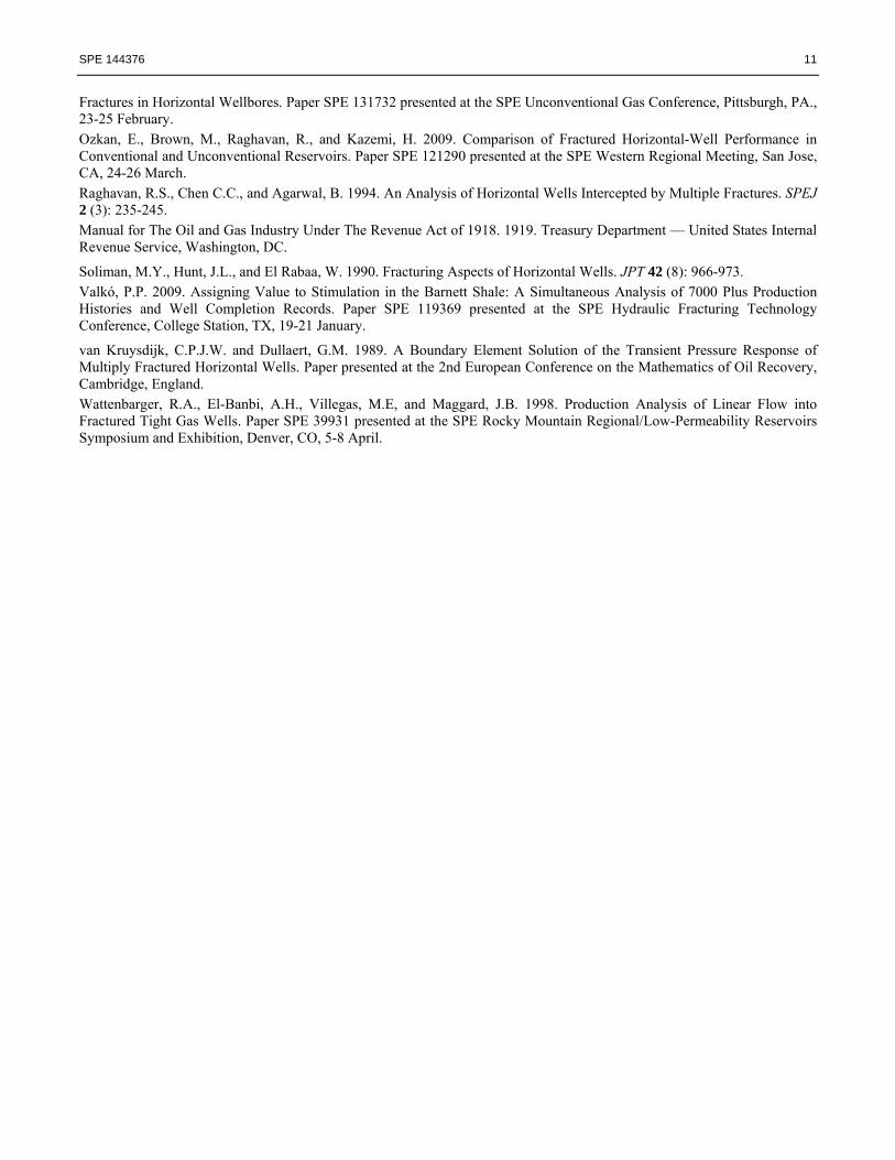
Fig. 1a — Production history plot for well 1. Flowrate and calculated bottomhole pressure versus time.
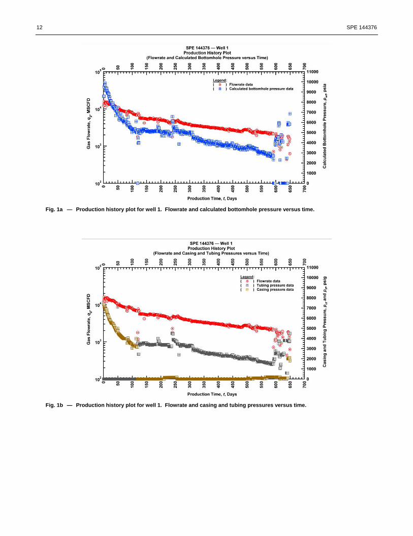
Fig. 1b — Production history plot for well 1. Flowrate and casing and tubing pressures versus time.
SPE 144376 13
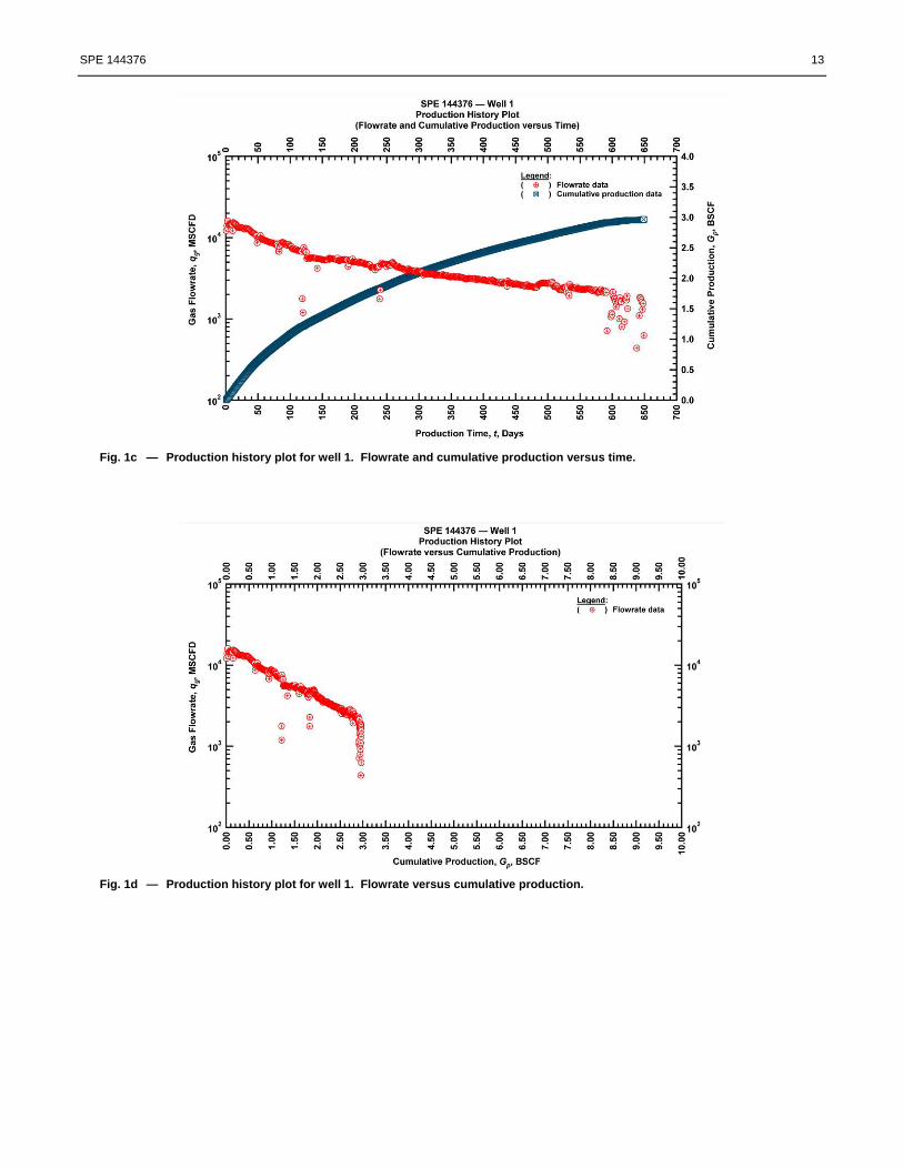
Fig. 1c — Production history plot for well 1. Flowrate and cumulative production versus time.
Fig. 1d — Production history plot for well 1. Flowrate versus cumulative production.

14 SPE 144376
Fig. 1e — Production history plot for well 1. Flowrate versus calculated bottomhole pressures.
Fig. 2a — Production history plot for well 2. Flowrate and calculated bottomhole pressure versus time.

SPE 144376 15
Fig. 2b — Production history plot for well 2. Flowrate and casing and tubing pressures versus time.
Fig. 2c — Production history plot for well 2. Flowrate and cumulative production versus time.

16 SPE 144376
Fig. 2d — Production history plot for well 2. Flowrate versus cumulative production.
Fig. 2e — Production history plot for well 2. Flowrate versus calculated bottomhole pressures.
SPE 144376 17
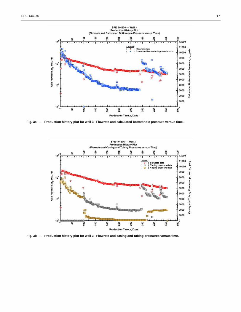
Fig. 3a — Production history plot for well 3. Flowrate and calculated bottomhole pressure versus time.
Fig. 3b — Production history plot for well 3. Flowrate and casing and tubing pressures versus time.

18 SPE 144376
Fig. 3c — Production history plot for well 3. Flowrate and cumulative production versus time.
Fig. 3d — Production history plot for well 3. Flowrate versus cumulative production.

SPE 144376 19
Fig. 3e — Production history plot for well 3. Flowrate versus calculated bottomhole pressures.
Fig. 4a — Production history plot for well 4. Flowrate and calculated bottomhole pressure versus time.

20 SPE 144376
Fig. 4b — Production history plot for well 4. Flowrate and casing and tubing pressures versus time.
Fig. 4c — Production history plot for well 4. Flowrate and cumulative production versus time.

SPE 144376 21
Fig. 4d — Production history plot for well 4. Flowrate versus cumulative production.
Fig. 4e — Production history plot for well 4. Flowrate versus calculated bottomhole pressures.

22 SPE 144376
Fig. 5a — Production history plot for well 5. Flowrate and calculated bottomhole pressure versus time.
Fig. 5b — Production history plot for well 5. Flowrate and casing and tubing pressures versus time.
SPE 144376 23
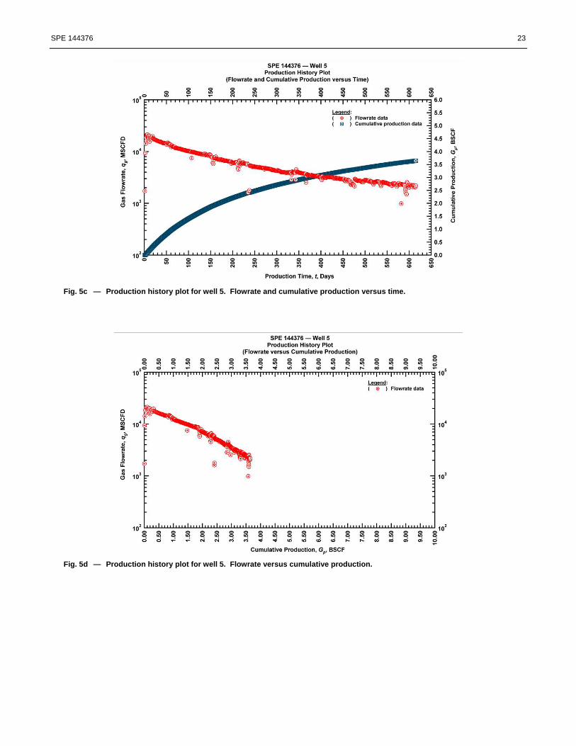
Fig. 5c — Production history plot for well 5. Flowrate and cumulative production versus time.
Fig. 5d — Production history plot for well 5. Flowrate versus cumulative production.

24 SPE 144376
Fig. 5e — Production history plot for well 5. Flowrate versus calculated bottomhole pressures.
Fig. 6a — Production history plot for well A. Flowrate and calculated bottomhole pressure versus time.

SPE 144376 25
Fig. 6b — Production history plot for well A. Flowrate and casing and tubing pressures versus time.
Fig. 6c — Production history plot for well A. Flowrate and cumulative production versus time.

26 SPE 144376
Fig. 6d — Production history plot for well A. Flowrate versus cumulative production.
Fig. 6e — Production history plot for well A. Flowrate versus calculated bottomhole pressures.

SPE 144376 27
Fig. 7a — Production history plot for well B. Flowrate and calculated bottomhole pressure versus time.
Fig. 7b — Production history plot for well B. Flowrate and casing and tubing pressures versus time.

28 SPE 144376
Fig. 7c — Production history plot for well B. Flowrate and cumulative production versus time.
Fig. 7d — Production history plot for well B. Flowrate versus cumulative production.

SPE 144376 29
Fig. 7e — Production history plot for well B. Flowrate versus calculated bottomhole pressures.
Fig. 8a — Production history plot for well C. Flowrate and calculated bottomhole pressure versus time.

30 SPE 144376
Fig. 8b — Production history plot for well C. Flowrate and casing and tubing pressures versus time.
Fig. 8c — Production history plot for well C. Flowrate and cumulative production versus time.
SPE 144376 31
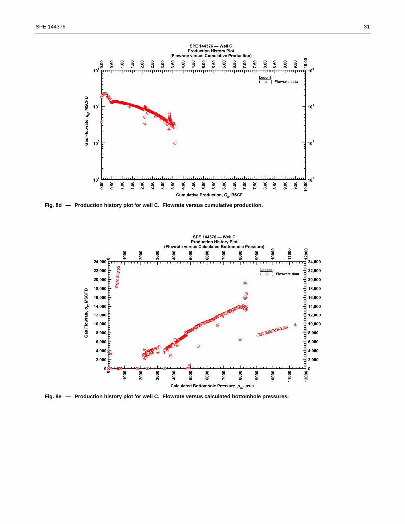
Fig. 8d — Production history plot for well C. Flowrate versus cumulative production.
Fig. 8e — Production history plot for well C. Flowrate versus calculated bottomhole pressures.

32 SPE 144376
Fig. 9a — Production history plot for well D. Flowrate and calculated bottomhole pressure versus time.
Fig. 9b — Production history plot for well D. Flowrate and casing and tubing pressures versus time.

SPE 144376 33
Fig. 9c — Production history plot for well D. Flowrate and cumulative production versus time.
Fig. 9d — Production history plot for well D. Flowrate versus cumulative production.

34 SPE 144376
Fig. 9e — Production history plot for well D. Flowrate versus calculated bottomhole pressures.
Fig. 10a — Reservoir diagnostics plot for all wells. Pressure drop normalized rate versus production time (log-log scale).

SPE 144376 35
Fig. 10b — Reservoir diagnostics plot for all wells. Pressure drop normalized rate versus material balance time (log-log scale).
Fig. 10c — Reservoir diagnostics plot for all wells. Pressure drop normalized rate versus square root of production time (log-log scale).
36 SPE 144376
Fig. 11a — Reservoir diagnostics plot for all wells. Pressure drop normalized rate versus cumulative production (Cartesian scale).
Fig. 11b — Reservoir diagnostics plot for all wells. Pressure drop normalized rate versus cumulative production (Log-log scale).

SPE 144376 37
Fig. 12a — Reservoir diagnostics plot for all wells. Pressure drop normalized cumulative production versus production time (log-log scale).
Fig. 12b — Reservoir diagnostics plot for all wells. Pressure drop normalized cumulative production versus material balance time (log-log scale).

38 SPE 144376
Fig. 12c — Reservoir diagnostics plot for all wells. Pressure drop normalized cumulative production versus square root of production time (log-log scale).
Fig. 13a — Reservoir diagnostics plot for all wells. Rate normalized pressured drop versus production time (Cartesian scale).
SPE 144376 39
Fig. 13b — Reservoir diagnostics plot for all wells. Rate normalized pressured drop versus material balance time (Cartesian scale).
Fig. 13c — Reservoir diagnostics plot for all wells. Rate normalized pressured drop versus square root of production time (Cartesian scale).
40 SPE 144376
Fig. 14a — Reservoir diagnostics plot for all wells. Computed D-parameter versus production time (Log-log scale).
Fig. 14b — Reservoir diagnostics plot for all wells. Computed b-parameter versus production time (Log-log scale).

SPE 144376 41
Fig. 14c — Reservoir diagnostics plot for all wells. βq-cp-derivative versus production time (Log-log scale).
Fig. 15 — History match plot for well 5. Flowrate and calculated bottomhole pressure data versus time with model functions.

42 SPE 144376
Fig. 16 — History match plot for well D. Flowrate and calculated bottomhole pressure data versus time with model functions.
Fig. 17 — Characteristic well performance model forecast plot. Flowrate and cumulative production models versus time.
SPE 144376 43
Fig. 18a — Forecast plot. Effect of number of fractures on recovery. Flowrate versus production time.
Fig. 18b — Forecast plot. Effect of number of fractures on recovery. Cumulative production versus production time.

44 SPE 144376
Fig. 19a — Forecast plot. Effect of horizontal well length on recovery. Flowrate versus production time.
Fig. 19b — Forecast plot. Effect of horizontal well length on recovery. Cumulative production versus production time.
SPE 144376 45
Fig. 20a — Forecast plot. Effect of horizontal well length and number of fractures on recovery. Flowrate versus production time.
Fig. 20b — Forecast plot. Effect of horizontal well length and number of fractures on recovery. Cumulative production versus production time.

46 SPE 144376
Fig. 21a — Forecast plot. Effect of well spacing on recovery. Flowrate versus production time.
Fig. 21b — Forecast plot. Effect of well spacing on recovery. Cumulative production versus production time.