Soil & Tillage Research 144 (2014) 174–183

Spatial variation of soil nutrients on sandy-loam soil

Igor Bogunovic *, Milan Mesic, Zeljka Zgorelec, Aleksandra Jurisic, Darija BilandzijaUniversity of Zagreb, Faculty of Agriculture, Department of General Agronomy, Svetošimunska cesta 25, 10000 Zagreb,Croatia

A R T I C L E I N F O

Article history:Received 15 April 2014Received in revised form 10 June 2014Accepted 29 July 2014

Keywords:GeostatisticsNutrient mapsInterpolation modelsSpatial variability

A B S T R A C T

The spatial variability of plant available phosphorus, plant available potassium, soil pH and soil organicmatter content in central Croatia was investigated using geostatistical tools and geographicalinformation system to create nutrient maps and provide useful information for the application ofinputs that will also be used for the design of an adequate soil sampling scheme. In a regular grid(50 m � 50 m), 330 samples were collected on sandy loam Stagnic Luvisol. Soil available phosphorus andplant available potassium showed relatively high spatial heterogeneity, ranging from 105 mg kg�1 to310 mg kg�1, and from 115 mg kg�1 to 462 mg kg�1, respectively. Content of soil organic matter and pHhad lower variability ranging from 1.26% to 2.66% and from 3.75 to 7.13, respectively. Investigated soilproperties did not follow normal distribution. Logarithm and Box–Cox transformation were applied toachieve normality. Directional exponential model for soil available phosphorus, potassium and pH andspherical model for soil organic matter was used to describe spatial autocorrelation. Fourteen differentinterpolation models for mapping soil properties were tested to compare the prediction accuracy. Allmodels gave similar root mean square error values. Available phosphorus, potassium and pH evaluated byradial basis function models (CRS, IMTQ and CRS, respectively) provide a more realistic picture of thestructures of analyzed spatial variables in contrast to kriging and inverse distance weighting models. Forsoil organic matter datasets the most favorable model was LP1. According to the best model soil nutrientmaps were created to provide guidance for site-specific fertilization and liming. Soil fertility mapsshowed sufficient concentrations of soil available phosphorus and available potassium. Acidity mapshowed that the largest part of the investigated area is very acid and acid. For future management it isnecessary to provide more liming materials while fertilization rate should be lower.

ã 2014 Elsevier B.V. All rights reserved.

Contents lists available at ScienceDirect

Soil & Tillage Research

journal homepage: www.else vie r .com/locate /s t i l l

1. Introduction

Nowadays, the vast majority of farmers in Croatia usefertilizers without analyzing the soil fertility. Just a minority offarmers use fertilizers according to soil analysis but withoutconsidering in-field spatial variability. In recent decades betterinvestigation methods resulted in higher awareness of crop andsoil science and soil properties variability within fields. Most ofthe yield variability studies have focused on soil nutrientavailability and less on soil physical property variability(Castrignano et al., 2002). In contrast to texture and soil organicmatter content, nutrients (e.g., potassium, phosphorus) havehigher temporal change in soils depending on soil or cropproperty (Heege, 2013). Therefore, it is necessary to monitor the

* Corresponding author. Tel.: +385 1 2393815.E-mail addresses: ibogunovic@agr.hr (I. Bogunovic), mmesic@agr.hr (M. Mesic),

zzgorelec@agr.hr (Z. Zgorelec), ajurisic@agr.hr (A. Jurisic), dbilandzija@agr.hr(D. Bilandzija).

http://dx.doi.org/10.1016/j.still.2014.07.0200167-1987/ã 2014 Elsevier B.V. All rights reserved.

condition of the soil in a shorter period of time which raises theoperating costs. Present technology allows us to improve theapplication of fertilizers and other inputs by varying rates andblends as needed within fields (Robert, 2002). Geostatisticalconcept with properly applied sampling trough interpolationtechnique allows us to assess the value of a soil property atunsampled locations within the area covered by observationpoints. Respecting the principles of regionalized variable theory(Clark, 1979; Journel and Huijbregts, 1978; Matheron, 1963) it ispossible to find the necessary dependence between two samplingpoints in space. But mapping the spatial distribution of nutrientsneeds better spatial interpolation methods and their compar-isons. Papers that compare different interpolations methods havealready been published (Pereira et al., 2013a,b; Robinson andMetternicht, 2006; Xie et al., 2011; Yang et al., 2004; Yasrebi et al.,2009) but the results are not clear. Studies reported differentdistances between dependent sampling points. Fu et al. (2010)found ranges of 264 m, 300 m and 290 m for phosphorus,potassium and pH on grassland. Robinson and Metternicht(2006) in topsoil of dryland paddock reported ranges of 2110 m

I. Bogunovic et al. / Soil & Tillage Research 144 (2014) 174–183 175

and 273 m for pH and organic matter, while Kravchenko andBullock (1999) recorded spatially dependent sampling pointsfrom 82 m to 608 m for phosphorus and 85 m to 532 m forpotassium in 30 different agricultural fields. Montanari et al.(2012) reported different spatially dependent ranges for phos-phorus depending of soil type. Two ranges were 1419 m onAlfisols and 689 m on Alfisols and Oxisols. On colluvial andalluvial soils in regular grid 500 m � 500 m Sa�glam et al. (2011)recorded spatial dependent ranges for soil organic matterbetween 809 and 1680 m depending on soil type. Someresearchers prefer ordinary kriging (Kravchenko and Bullock,1999; Laslett et al., 1987), others (Gotway et al., 1996; Weber andEnglund, 1992) inverse distance weighting (IDW) and splines(Robinson and Metternicht, 2006) depending on the investigatedparameters, distance between sampling points, dealing with datatransformation and the number of neighborhood data pointsused. Furthermore, interpolation is always associated with somedegree of uncertainty, because estimation of an unsampled pointproduces some error, independent of the method used (Ahmedet al., 2011). The purpose of this study was to investigatestatistical methods to describe the observed spatial patterns ofsoil available potassium (AK), available phosphorus (AP), soilacidity (pH) and soil organic matter (SOM). By comparing the

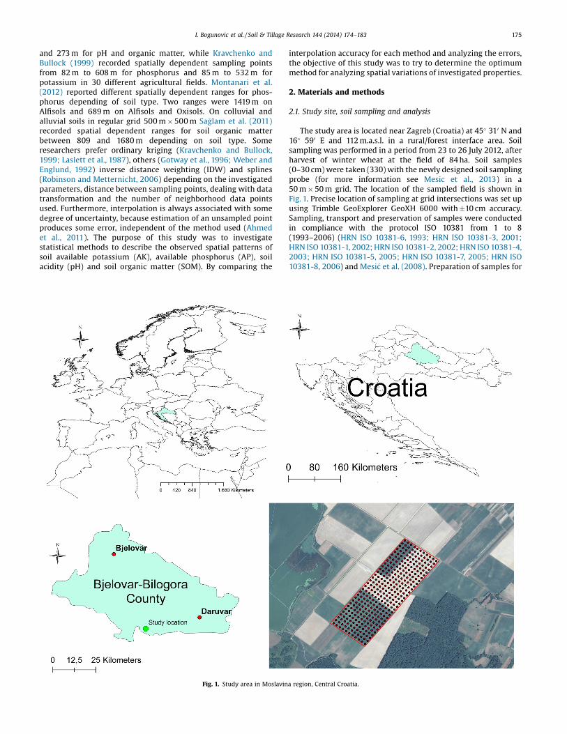
Fig. 1. Study area in Moslavin

interpolation accuracy for each method and analyzing the errors,the objective of this study was to try to determine the optimummethod for analyzing spatial variations of investigated properties.

2. Materials and methods

2.1. Study site, soil sampling and analysis

The study area is located near Zagreb (Croatia) at 45� 310 N and16� 590 E and 112 m.a.s.l. in a rural/forest interface area. Soilsampling was performed in a period from 23 to 26 July 2012, afterharvest of winter wheat at the field of 84 ha. Soil samples(0–30 cm) were taken (330) with the newly designed soil samplingprobe (for more information see Mesic et al., 2013) in a50 m � 50 m grid. The location of the sampled field is shown inFig. 1. Precise location of sampling at grid intersections was set upusing Trimble GeoExplorer GeoXH 6000 with �10 cm accuracy.Sampling, transport and preservation of samples were conductedin compliance with the protocol ISO 10381 from 1 to 8(1993–2006) (HRN ISO 10381-6, 1993; HRN ISO 10381-3, 2001;HRN ISO 10381-1, 2002; HRN ISO 10381-2, 2002; HRN ISO 10381-4,2003; HRN ISO 10381-5, 2005; HRN ISO 10381-7, 2005; HRN ISO10381-8, 2006) and Mesi�c et al. (2008). Preparation of samples for

a region, Central Croatia.

176 I. Bogunovic et al. / Soil & Tillage Research 144 (2014) 174–183

chemical analysis (drying, milling, sieving, homogenizing) wasconducted in compliance with protocol HRN ISO 11464 (2004). SoilpH was measured using the electrometric method in 1:5 (w/v)ratio with the Beckman pH-meter F72, in Kl suspension (HRN ISO10390, 2005). AP and AK were extracted by ammonium lactate (AL)solution (Egner et al., 1960) and detected by spectrophotometricand flame photometric, respectively. In all soil samples mass ratioof SOM was analyzed using dry combustion method (HRN ISO10694, 2004) with the vario MACRO CHNS analyzer in theAnalytical laboratory of the Department of General Agronomy,Faculty of Agriculture University of Zagreb.

The soil is classified as Pseudogley according to Croatianclassification (Škori�c et al., 1973) or Stagnic Luvisols according toWRB classification (FAO, 2006). By its texture the soil on theexperimental field belongs to sandy loam (Table 1). Climate is semihumid to humid with annual precipitation (in referent period1960–1991) of 863 mm and average annual temperature of 10.7 �C(Meteorological and hydrological Service of Croatia – meteorolog-ical station in Daruvar, 15 km away from investigated area).

Usual crop rotation in that area is winter wheat, maize, soybean,barley and oilseed rape. Soil sampling was performed after winterwheat harvest.

2.2. Statistical analyses and data transformation

Some basic statistics were analyzed, such as minimum (min),5th percentile (5%), 1st quantile (25%), median, 3rd quantile (75%),95th percentile (95%), maximum, mean values and the coefficientof variation (CV). The descriptive parameters were calculated usingMicrosoft Excel for Windows. The Kolmogorov–Smirnov (K–S) testand Q–Q plots were created to analyze the data distribution andpotential outliers using SAS software (Version 9.3). The K–Smethod, the skewness and kurtosis evaluate data normality andasymmetry that have important implications on interpolationmethods performance.

Data were subjected to quality control before modeling. In orderto achieve a correct interpretation of the spatial interpolation, it isdesirable to have data as close as possible to the normaldistribution (Clark and Harper, 2000; Goovaerts et al., 2005;McGrath et al., 2004). High skewness and the presence of outlierscan have negative consequences on the accuracy and semivario-gram interpretation. To avoid these problems raw data were testedand transformed when necessary. The most common methodswere logarithmic (log) and Box–Cox (BC) transformations used tonormalize data sets (Fu et al., 2010; Thayer et al., 2003). Logtransformations are commonly used to normalize positive skeweddata (McGrath et al., 2004) but this transformation was not enoughon some occasions. In order to improve data when log transfor-mation fails, BC transformation is more powerful and widely usedmethod (Box and Cox, 1964; Gallardo and Paramá, 2007).

2.3. Geostatistical analysis

In this study geostatistics was used to describe spatial variationof each investigated soil property. Spatial patterns of nutrientswere observed with the experimental semivariogram modelingusing the data developed to identify the spatial continuity of AP,

Table 1Particle size distribution on Stagnic Luvisols (from Kisi�c et al., 2002)

Soil depth (cm) Soil horizon Texture (g kg�1)

Coarse sand (2–0.2 mm) Fine sand (0.2–

0–24 Ap + Eg 18 586

24–35 Eg + Btg 21 571

35–95 Btg 5 545

AK, pH and SOM among sampling points. Semivariogram assistsdissimilarity between paired data values to the distance betweeneach sample pair (Goovaerts, 1997; Webster and Oliver, 2007) andgives the spatial structure of the variable and the correlation withthe closest points. There are some frequently used models todescribe experimental semivariograms: spherical, exponential,Gaussian and linear (Isaaks and Srivastava, 2011).

Semivariogram can be expressed as:

gðhÞ ¼ 12NðhÞ

XNðhÞi¼1

ZðxiÞ � Zðxi þ hÞ½ �2

where g(h) is the semivariance at a given distance h; Z(xi) is thevalue of the variable Z at the xi location and N(h) is the number ofpairs of sample points separated by the lag distance h.

For spatial data, semivariance increases with the distances thatare correlated and if the variogram stabilizes it reaches the sill(C + C0), showing that at distance x the samples are consideredspatially independent. The variance observed at a shorter scalethan the field sampling is identified at 0 lag distance, known as thenugget effect – C0. This nugget effect makes the short-scalevariability and/or sampling errors evident (Burgos et al., 2006;Cetin and Kirda, 2003; Fu et al., 2010). In this study the modeledsemi variograms are directional. According previous studies(Webster and Oliver, 2007; Robinson and Metternicht, 2006)number of required sampling points is higher than minimum (150)to reliably identify the presence of anisotropy which considers thatthe variability is not equal in all directions. In order to describe thedirectional semi variogram, direction were tested from 0 to 360 by5 to achieve highest range with applied angular tolerance of 45�.Variable spatial dependency was calculated by the nug/sill ratio. Ifthe ratio is lower than 25%, the variable has strong spatialdependence; if it is between 25% and 75%, the variable hasmoderate spatial dependence; and if it is higher than 75% thevariable shows only weak spatial dependence (Chien et al., 1997).Normally, strong spatial dependence is attributed to intrinsicfactors and weak spatial dependence is attributed to extrinsicfactors (Cambardella et al., 1994).

The interpolation method is recognized as a key factor forinterpolation accuracy. Comparison and accuracy of interpolationmethods has been investigated in several studies. The reliability ofthe interpolation gives a better assessment of the spatialdistribution of the variables (Robinson and Metternicht, 2006;Shi et al., 2009; Wu et al., 2011). Interpolation methods can bedivided in three categories: (1) statistics – with regression tree andmultiple regression; (2) geostatistics that include ordinary krigingand universal kriging, and (3) hybrid with co-kriging andregression kriging. Present study tested following interpolationmethods that are part of the ArcGIS software: inverse distance to aweight (IDW) with the power of 1–5, local polynomial, radial basisfunctions (RBF)—spline with tension, completely regularizedspline, multiquadratic, inverse multiquadratic and thin platespline (TPS)—and two geostatistical methods, ordinary kriging(OK) and simple kriging (SK). They are commonly used in theliterature (Erdogan, 2009; Pereira et al., 2013a,b; Xie et al., 2011). Ineach interpolation a total of fifteen neighbors were included and asmoothed value of 0.5 was applied.

Texture class

0.02 mm) Silt (0.02–0.002 mm) Clay (<0.002 mm)

242 154 Sandy loam260 148 Sandy loam254 196 Sandy loam

I. Bogunovic et al. / Soil & Tillage Research 144 (2014) 174–183 177

Accuracy assessment was carried out with cross-validationmethod previously used in papers Erxleben et al. (2002), Kerryet al. (2012), Robinson and Metternicht (2006). This methodcompares the observed values with the predicted ones. Cross-validation was obtained by taking each observation in turn out ofthe sample pool and estimating from the remaining ones. Theerrors produced, between observed and predicted values, are usedto evaluate the performance of each method. With these data, themean error (ME) and root mean square error (RMSE) werecalculated. The ME is calculated with the following formula:

ME ¼ 1NSn

i¼1ZðXiÞ �Z Xið Þ

n oRoot mean square error is calculated following this formula:

RMSE ¼ffiffiffiffiffiffiffiffiffiffiffiffiffiffiffiffiffiffiffiffiffiffiffiffiffiffiffiffiffiffiffiffiffiffiffiffiffiffiffiffiffiffiffiffiffiffi1NSn

i¼1ZðXiÞ �Z Xið Þ

n o2s

where Z(Xi) is the observed value, Z ðXiÞ is the predicted value andN is the number of samples.

The best method was the one which had the lowest RMSE.Differencesand correlationsbetweenobservedandestimatedvalueswere identified with the paired t-test and Pearson correlation andconsidered significant at p < 0.05. Statistical analyses were carriedout with SAS software (Version 9.3) and the semi-variogram andinterpolationmethodsanalysiswithArcGis10.0(ESRI)forWindows.

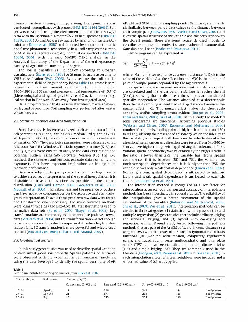
Fig. 2. Normal Q–Q plots for original data (n = 330). From

3. Results and discussion

3.1. Q–Q plots, descriptive parameters and normality test

In order to observe normality and analyze original datadistribution normal Q–Q plots were created (Fig. 2). All investigat-ed factors showed non-normal distribution. One abnormally highvalue was observed in AK (1090 mg kg�1) at a site located close tothe field entrance near channels. Apart from this extreme in AKpopulation, only few other samples deviated at both ends. Soil APand SOM lined up in a near straight line, but indicated some degreeof left skewed distribution. A certain pattern is visible in soil pH,but the skewness is more strongly expressed. AK and pH recordedsome changes in slope which are slightly more numerous thanwith the other factors.

Percentiles and classical descriptive parameters were calculat-ed and are shown in Table 2. The current average contents of AP, AK,pH and SOM at 0–30 cm depth in the Pseudogley soil area were189.1 mg kg�1, 216.7 (214.0) mg kg�1, 4.54 and 1.72%, respectively.Among the presented statistical data, CV value is the mostdiscriminating factor for describing variability. CV value which islower than 10% indicates low variability while CV value above 90%shows extensive variability (Zhang et al., 2007). All investigatedparameters recorded moderate variability, while the highestvariability was observed in AK with CV value of 32.64%. Theseresults contain an outlier, but after removing that extreme data

the upper left to lower right: AK, AP, SOM and pH.

Table 2Univariate statistics for AP (mg kg�1), AK (mg kg�1), pH and SOM (%).

Min 5% 25% Median 75% 95% Max Mean CV(%)

AP 105.8 132.3 158.2 182.3 210.7 278.1 310.3 189.1 22.06AK 115.9 139.9 176.6 206.6 249.0 294.2 1090.0 (462.7) 216.7 (214.0) 32.64 (24.21)pH 3.75 3.98 4.15 4.33 4.71 6.05 7.14 4.56 14.29SOM 1.26 1.43 1.57 1.69 1.83 2.10 2.66 1.72 12.82

Mean and CV values in brackets were calculated without AK outlier.

178 I. Bogunovic et al. / Soil & Tillage Research 144 (2014) 174–183

(1090 mg kg�1) from the statistical analysis, CV was 24.21%, whichis still higher than the CV value observed in other investigatedproperties.

After removing the outlier, AK skewness changed from 6.08 to0.98 and kurtosis reduced from 70.42 to 2.49. This great change inthe shape of the parameters is the reason for removing the outlierin order to obtain the characteristics of the majority of data.According to Barnett and Lewis (1994) outliers can cause distortionthat violates geostatistical theory. Their influence on statisticalanalysis should be limited and will be removed for variogramanalysis in this study. For kriging analysis outlier will be replacedwith the maximum value, because an outlier can make variogramerratic (Armstrong and Boufassa, 1988). Both investigated soilnutrients (AK and AP) showed higher spatial heterogeneity incontrast to pH and SOM, but these values are far from theheterogeneity presented in papers by Fu et al. (2010), Kravchhenko(2003), Liu et al. (2009) and Schloeder et al. (2001) with CV valueabove 35%. Other investigated soil properties have also recordedvariations. AP and AK heterogeneity could be attributed to unevenfertilizer usage or soil erosion. The CV value of SOM was only12.82%. SOM is usually considered a relatively stable variable, withminimum variation. The SOM content in the soil usually varies andis associated with the severity of pedogenesis process. pHvariations were relatively small with CV value of 14.29%. Otherresearchers (Castrignanò et al., 2000; Chung et al., 1995; Fu et al.,2010; McBratney and Webster, 1983; Parfitt et al., 2009) also reportrelatively small variations of pH of the surface layer with CV valuefrom 2.22% (Castrignanò et al., 2000) to 8.1% (Fu et al., 2010). Thisrelatively stabile and persistent distribution of SOM and pH ispreferred for the application of lime materials and organic mattermanagement.

The original data did not pass the K–S test for normality(p = 0.05). The data were highly skewed (Table 3), and this can beobserved in the shape of Q–Q plots (Fig. 2). After the logtransformations, data confirm the Gaussian distribution for APand AK, while pH and SOM did not follow normal distribution.After the Box–Cox transformation data were closer to the Gaussiandistribution, but still they did not follow the normality in pHcontent, while SOM content followed a normal distribution.However, values of pH data after Box–Cox transformation incontrast to previous transformations, were closer to the normaldistribution, and the skewness and kurtosis were closer to 0. Thissituation is not unheard of and is evidenced in McGrath and Zhang(2003) study. They observed that after log data transformation, pHvalues did not pass the K–S test, but authors modeled the variable

Table 3Shape parameters and K–S test for original and transformed data.

Original data Log-transformed data

Skewness Kurtosis K–S Skewness Kurtosp

AP 0.71 0.21 <0.01 0.18 �0.29AK 0.98 2.49 <0.01 0.14 �0.01pH 2.03 4.29 <0.01 1.64 2.66SOM 1.05 2.09 <0.01 0.55 0.90

Parameters for AK were calculated without the outlier.

with log transformed data. In this study, pH dataset showedsmaller skewness and kurtosis after Box–Cox transformation andthese data were used for modeling. If data cannot be modeled witha normal distribution, they should at least be as close to the normaldistribution as possible (Zhang, 2006). Pereira et al. (2013a,b)follow a similar procedure in studies with ash thickness modeling.Therefore, the log-transformed data sets of AP and AK, and theBox–Cox transformed data sets of SOM and pH were used for thefollowing multivariate analyses.

3.2. Spatial characteristics of investigated properties

The parameters for variogram models are listed in Table 4 andthe fitted variogram plots for AK, AP, SOM and pH are shown inFig. 3. All variogram models recorded directional differences whichindicate differently increased variogram values at differentdirections. The longest range spatial dependence for AP, AK,SOM and pH was found in directions 40, 25, 85 and 70, respectively.Among other models, the exponential model gave the best fit forthe experimental variograms calculated for AP, AK and pH (Fig. 3a,b and d). Nugget effect was not recorded for soil AP while therecorded nugget for AK and pH was 0.00427 and 0.00001,respectively. Compared to sill, small nugget values indicate thatsampling errors are negligible. Usually the nugget effect occurs as aconsequence of limited sample numbers, small-scale variance andthe existence of outliers (Gringarten and Deutsch, 2001; McGrathand Zhang, 2003). In present study, the number of samples wasrepresentative of the studied plot, and the outlier in AK wasreplaced with the maximum value. Thus, the nugget effect wasattributed to the small-scale variance observed in some areas ofthe plot in the current sampling density.

AP and pH variable with nugget/sill ratio of 0.00 and 19.54,respectively, showed strong spatial dependence, while AK with a36.33 nugget/sill ratio showed moderate spatial dependence. Thespherical model fitted to the experimental variogram calculatedfor SOM data (Fig. 3c) recorded a nugget effect of 0.00223 and a sillof 0.00320 along a range of 864.0 m. The nugget/sill ratio (69.56)showed that SOM had a moderate spatial dependence. Ranges of allinvestigated parameters were much wider than the samplinginterval of 50 m. According to the geostatistical theory, thissampling design is sufficient for the investigation of spatialdependence and distribution of investigated parameters in theinvestigated soil.

Kerry and Oliver (2004) indicated that a rough guide forchoosing future sampling interval should be less than half the

Box–Cox transformation

is K–S Lambda Skewness Kurtosis K–Sp p

>0.15 >0.15

<0.01 �2 0.98 0.55 <0.01 <0.01 �1.5 �0.13 0.51 >0.15

Table 4Best-fitted anisotropic variogram models of AP, AK, SOM and pH and corresponding parameters.

Model Nugget C0 Partial sill C Sill C0 + C Nugget/Sill Range (meters)

AP Exponential 0.00000 0.00718 0.00718 0.00 201.3AK Exponential 0.00427 0.00749 0.01177 36.33 1153.6SOM Spherical 0.00223 0.00097 0.00320 69.56 864.0pH Exponential 0.00001 0.00003 0.00004 19.45 1954.4

I. Bogunovic et al. / Soil & Tillage Research 144 (2014) 174–183 179

variogram range. According to the results of this study futuresampling grid should be at least 100 m for AP and 400 m formonitoring AK and SOM. Suitable sampling interval of 100 m for APis also suggested in papers by Mallarino et al. (2006) and Fu et al.(2010) in 30 m grid intervals and 150 m interval is suggested for AK(Fu et al., 2010). Soil pH shows incredible high range (1954.4 m)and significant spatial dependence (nugget/sill 19.45). Soil of theinvestigated area has naturally low pH regardless of theenvironmental and topographical factors. The results of this studyshowed that 90% of samples are very acid (pH < 4.5) and acid (pHfrom 4.5 to 5.5) and this is the reason for high spatial homogeneityof soil pH that resulted in high range in variogram. This pH value isa great warning and indicates the limitations of these soils foragricultural production. In future production period significantamount of liming materials will be needed to improve soil pH.

Current soil sampling strategy in Croatia is unclear, insufficientfor the continuous monitoring of soil and is performed by only asmall number of corporations. It is mostly done as onerepresentative sample made by 20 soil cores in a zigzag patternfrom a 5 ha field area. According to the results of this study thissampling method may not be adequate for proper agricultural soil

Fig. 3. Directional semi-variogram calculated for AP (a) and AK (b) with log-transformedbest fit model.

monitoring and does not provide enough accurate information forfertilizer and lime application. Taking into account the constantproblems with the cost of precise sampling, sampling scheme on100 m to a maximum of 150 m, depending of the soil type, past landuse and topographic factors, can be recommended. Althoughcorresponding parameters of variogram models suggests a greaterdistance for samples, these must be taken into consideration withcaution because some important soil attributes may be missingunder natural soil variability when the grid size is too large.

3.3. Interpolation methods assessment and spatial distribution

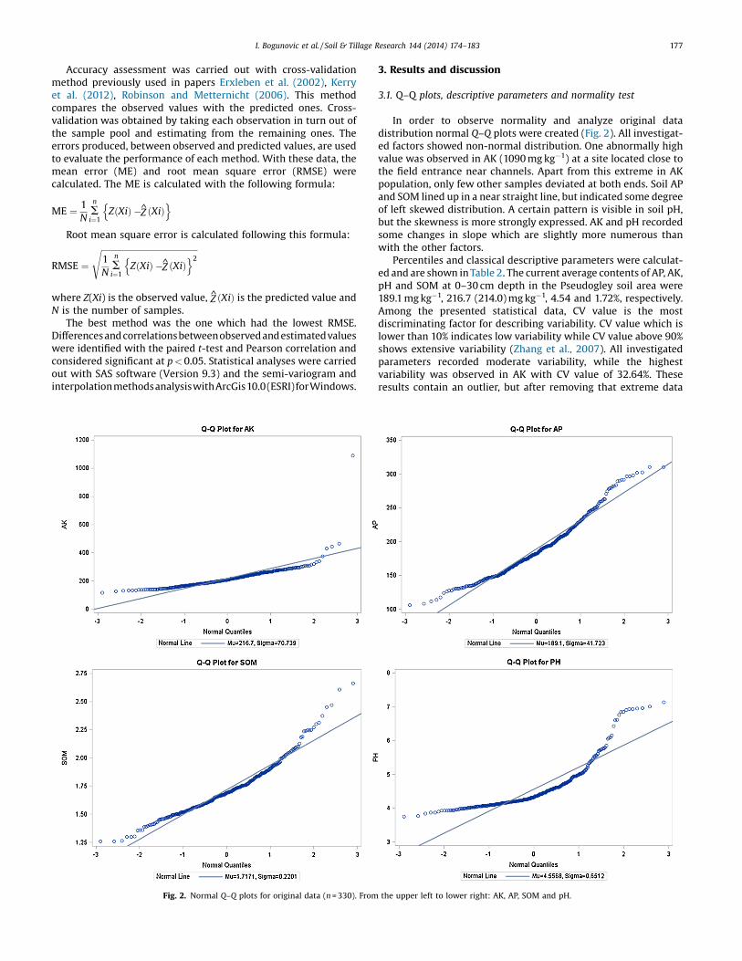
The results of the tested interpolation methods for allparameters are shown in Table 5. The test of the differentinterpolation methods provides an accurate insight in the spatialdistribution of AP, AK, SOM and pH on sandy loam soil. CRS methodwas the most accurate for interpolating the AP (RMSE, 0.0540) andthe least precise method was IDW1 (RMSE, 0.0812). The mostprecise method for AK was IMTQ (RMSE 0.0570) and the leastaccurate method was IDW1 (RMSE 0.0879). LP1 proved to be themost accurate method for SOM (RMSE 0.0473) and the least precise

data; SOM (c) and pH (d) with Box–Cox transformed data. Bold line represents the

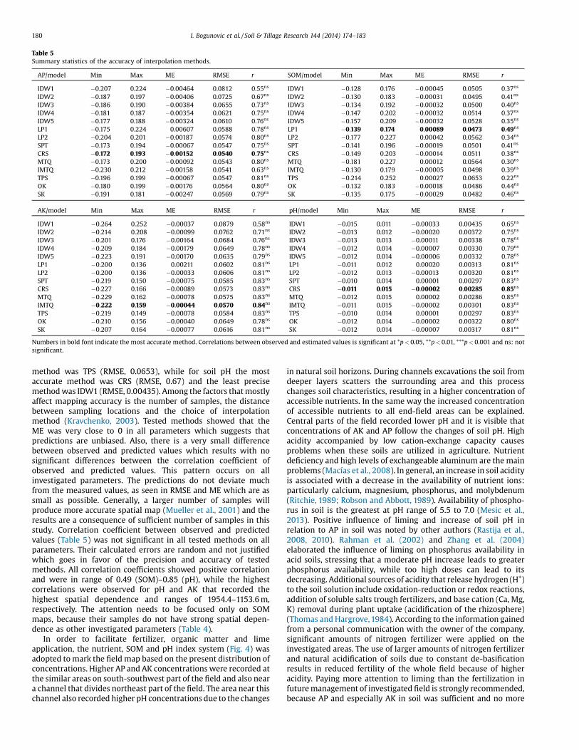
Table 5Summary statistics of the accuracy of interpolation methods.

AP/model Min Max ME RMSE r SOM/model Min Max ME RMSE r

IDW1 �0.207 0.224 �0.00464 0.0812 0.55ns IDW1 �0.128 0.176 �0.00045 0.0505 0.37ns

IDW2 �0.187 0.197 �0.00406 0.0725 0.67ns IDW2 �0.130 0.183 �0.00031 0.0495 0.41ns

IDW3 �0.186 0.190 �0.00384 0.0655 0.73ns IDW3 �0.134 0.192 �0.00032 0.0500 0.40ns

IDW4 �0.181 0.187 �0.00354 0.0621 0.75ns IDW4 �0.147 0.202 �0.00032 0.0514 0.37ns

IDW5 �0.177 0.188 �0.00324 0.0610 0.76ns IDW5 �0.157 0.209 �0.00032 0.0528 0.35ns

LP1 �0.175 0.224 0.00607 0.0588 0.78ns LP1 �0.139 0.174 0.00089 0.0473 0.49ns

LP2 �0.204 0.201 �0.00187 0.0574 0.80ns LP2 �0.177 0.227 0.00042 0.0562 0.34ns

SPT �0.173 0.194 �0.00067 0.0547 0.75ns SPT �0.141 0.196 �0.00019 0.0501 0.41ns

CRS �0.172 0.193 �0.00152 0.0540 0.75ns CRS �0.149 0.203 �0.00014 0.0511 0.38ns

MTQ �0.173 0.200 �0.00092 0.0543 0.80ns MTQ �0.181 0.227 0.00012 0.0564 0.30ns

IMTQ �0.230 0.212 �0.00158 0.0541 0.63ns IMTQ �0.130 0.179 �0.00005 0.0498 0.39ns

TPS �0.196 0.199 �0.00067 0.0547 0.81ns TPS �0.214 0.252 0.00027 0.0653 0.22ns

OK �0.180 0.199 �0.00176 0.0564 0.80ns OK �0.132 0.183 �0.00018 0.0486 0.44ns

SK �0.191 0.181 �0.00247 0.0569 0.79ns SK �0.135 0.175 �0.00029 0.0482 0.46ns

AK/model Min Max ME RMSE r pH/model Min Max ME RMSE r

IDW1 �0.264 0.252 �0.00037 0.0879 0.58ns IDW1 �0.015 0.011 �0.00033 0.00435 0.65ns

IDW2 �0.214 0.208 �0.00099 0.0762 0.71ns IDW2 �0.013 0.012 �0.00020 0.00372 0.75ns

IDW3 �0.201 0.176 �0.00164 0.0684 0.76ns IDW3 �0.013 0.013 �0.00011 0.00338 0.78ns

IDW4 �0.209 0.184 �0.00179 0.0649 0.78ns IDW4 �0.012 0.014 �0.00007 0.00330 0.79ns

IDW5 �0.223 0.191 �0.00170 0.0635 0.79ns IDW5 �0.012 0.014 �0.00006 0.00332 0.78ns

LP1 �0.200 0.136 0.00211 0.0602 0.81ns LP1 �0.011 0.012 0.00020 0.00313 0.81ns

LP2 �0.200 0.136 �0.00033 0.0606 0.81ns LP2 �0.012 0.013 �0.00013 0.00320 0.81ns

SPT �0.219 0.150 �0.00075 0.0585 0.83ns SPT �0.010 0.014 0.00001 0.00297 0.83ns

CRS �0.227 0.166 �0.00089 0.0573 0.83ns CRS �0.011 0.015 �0.00002 0.00285 0.85ns

MTQ �0.229 0.162 �0.00078 0.0575 0.83ns MTQ �0.012 0.015 0.00002 0.00286 0.85ns

IMTQ �0.222 0.159 �0.00044 0.0570 0.84ns IMTQ �0.011 0.015 �0.00002 0.00301 0.83ns

TPS �0.219 0.149 �0.00078 0.0584 0.83ns TPS �0.010 0.014 0.00001 0.00297 0.83ns

OK �0.210 0.156 �0.00040 0.0649 0.78ns OK �0.012 0.014 �0.00002 0.00322 0.80ns

SK �0.207 0.164 �0.00077 0.0616 0.81ns SK �0.012 0.014 �0.00007 0.00317 0.81ns

Numbers in bold font indicate the most accurate method. Correlations between observed and estimated values is significant at *p < 0.05, **p < 0.01, ***p < 0.001 and ns: notsignificant.

180 I. Bogunovic et al. / Soil & Tillage Research 144 (2014) 174–183

method was TPS (RMSE, 0.0653), while for soil pH the mostaccurate method was CRS (RMSE, 0.67) and the least precisemethod was IDW1 (RMSE, 0.00435). Among the factors that mostlyaffect mapping accuracy is the number of samples, the distancebetween sampling locations and the choice of interpolationmethod (Kravchenko, 2003). Tested methods showed that theME was very close to 0 in all parameters which suggests thatpredictions are unbiased. Also, there is a very small differencebetween observed and predicted values which results with nosignificant differences between the correlation coefficient ofobserved and predicted values. This pattern occurs on allinvestigated parameters. The predictions do not deviate muchfrom the measured values, as seen in RMSE and ME which are assmall as possible. Generally, a larger number of samples willproduce more accurate spatial map (Mueller et al., 2001) and theresults are a consequence of sufficient number of samples in thisstudy. Correlation coefficient between observed and predictedvalues (Table 5) was not significant in all tested methods on allparameters. Their calculated errors are random and not justifiedwhich goes in favor of the precision and accuracy of testedmethods. All correlation coefficients showed positive correlationand were in range of 0.49 (SOM)–0.85 (pH), while the highestcorrelations were observed for pH and AK that recorded thehighest spatial dependence and ranges of 1954.4–1153.6 m,respectively. The attention needs to be focused only on SOMmaps, because their samples do not have strong spatial depen-dence as other investigated parameters (Table 4).

In order to facilitate fertilizer, organic matter and limeapplication, the nutrient, SOM and pH index system (Fig. 4) wasadopted to mark the field map based on the present distribution ofconcentrations. Higher AP and AK concentrations were recorded atthe similar areas on south-southwest part of the field and also neara channel that divides northeast part of the field. The area near thischannel also recorded higher pH concentrations due to the changes

in natural soil horizons. During channels excavations the soil fromdeeper layers scatters the surrounding area and this processchanges soil characteristics, resulting in a higher concentration ofaccessible nutrients. In the same way the increased concentrationof accessible nutrients to all end-field areas can be explained.Central parts of the field recorded lower pH and it is visible thatconcentrations of AK and AP follow the changes of soil pH. Highacidity accompanied by low cation-exchange capacity causesproblems when these soils are utilized in agriculture. Nutrientdeficiency and high levels of exchangeable aluminum are the mainproblems (Macías et al., 2008). In general, an increase in soil acidityis associated with a decrease in the availability of nutrient ions:particularly calcium, magnesium, phosphorus, and molybdenum(Ritchie, 1989; Robson and Abbott, 1989). Availability of phospho-rus in soil is the greatest at pH range of 5.5 to 7.0 (Mesic et al.,2013). Positive influence of liming and increase of soil pH inrelation to AP in soil was noted by other authors (Rastija et al.,2008, 2010). Rahman et al. (2002) and Zhang et al. (2004)elaborated the influence of liming on phosphorus availability inacid soils, stressing that a moderate pH increase leads to greaterphosphorus availability, while too high doses can lead to itsdecreasing. Additional sources of acidity that release hydrogen (H+)to the soil solution include oxidation-reduction or redox reactions,addition of soluble salts trough fertilizers, and base cation (Ca, Mg,K) removal during plant uptake (acidification of the rhizosphere)(Thomas and Hargrove, 1984). According to the information gainedfrom a personal communication with the owner of the company,significant amounts of nitrogen fertilizer were applied on theinvestigated areas. The use of larger amounts of nitrogen fertilizerand natural acidification of soils due to constant de-basificationresults in reduced fertility of the whole field because of higheracidity. Paying more attention to liming than the fertilization infuture management of investigated field is strongly recommended,because AP and especially AK in soil was sufficient and no more

Fig. 4. Spatial distribution maps according to the most accurate technique. Left-to-right: first row: AP (CRS) and AK (IMTQ) with log-transformed data. Second row: SOM (LP1)and pH (CRS) with Cox–Box transformed data.

I. Bogunovic et al. / Soil & Tillage Research 144 (2014) 174–183 181

phosphorus and potassium fertilizer is needed. Concentrations ofSOM are the most favorable on the northern part of the field andnear the field edges, more or less following the spatial dispositionof pH. SOM concentration strongly depends on plant residuesmanagement, crop rotation, climate, nitrogen availability andmicrobiological activity in soil. Tillage operations and climate arethe same at the whole field and thus a conclusion can be drawnthat the pH, indirectly through soil conditions, directly affects themicrobial activity and regeneration of humic particles.

4. Conclusions

Investigated parameters do not follow normal distribution. Theapplication of log–and Cox–Box transformations was effective inshifting the data sets to normality with acceptable skewnessvalues. For AP, AK and pH best variogram fitted model was

exponential. The spatial structure of SOM was fitted by sphericalmodel. Practical application of research results comes from the factthat the inclusion of established models directional semivario-grams in interpolation analysis can improve the reliability of localassessments of the analyzed soil properties at unsampledlocations, thus reducing the cost of the production cycle. Allinvestigated parameters (AP, AK, SOM and pH) recorded higherrange than sampling interval with 201.3, 1153.6, 864.0 and1954.4 m, respectively. In order to reduce production costs asampling interval of 100 to 150 m is recommend, depending on theparameter. However, since all of the parameters are measured fromthe same soil samples, the recommended interval is 100 m. Alltested interpolation methods have high prediction accuracy of themean content. Models of spatial distribution of AP, AK and pHdatasets evaluated by RBF (CRS, IMTQ and CRS) models provide amore realistic picture of the structures of analyzed spatial variables

182 I. Bogunovic et al. / Soil & Tillage Research 144 (2014) 174–183

in contrast to kriging and IDW models. For SOM datasets the mostfavorable model was LP1. This indicates that prior to theimplementation of the development of distribution maps,parameters of semivariograms need to be computed. These resultslead to a conclusion that non interpolator can produce results forcontinuous monitoring of certain soil property. All investigatedmodels provide small RMSE and ME but it is necessary to achievethe smallest error in prediction to avoid economic cost. The use ofinterpolation methods and geostatistics proved a possibility toachieved enough accurate fertility maps to provide correctinformation for site specific fertilization and liming application.This will in turn result in reduced use of fertilizers, favorable soilreaction, increased soil microbial activity and will reduce potentialenvironmental problems.

Appendix A. Supplementary data

Supplementary data associated with this article can be found, inthe online version, at http://dx.doi.org/10.1016/j.still.2014.07.020.

References

Ahmed, Z.U., Panaullah, G.M., DeGloria, S.D., Duxbury, J.M., 2011. Factors affectingpaddy soil arsenic concentration in Bangladesh: prediction and uncertainty ofgeostatistical risk mapping. Sci. Total Environ. 412, 324–335.

Armstrong, M., Boufassa, A.,1988. Comparing the robustness of ordinary kriging andlognormal kriging: outlier resistance. Math. Geol. 20 (4), 447–457.

Barnett, V., Lewis, T., 1994. Outliers in Statistical Data, third ed. Wiley, New York.Box, G.E., Cox, D.R., 1964. An analysis of transformations. J. Roy. Stat. Soc. B 26 (2),

211–252.Burgos, P., Madejón, E., Pérez-de-Mora, A., Cabrera, F., 2006. Spatial variability of the

chemical characteristics of a trace-element-contaminated soil before and afterremediation. Geoderma 130 (1), 157–175.

Cambardella, C.A., Moorman, T.B., Novak, J.M., Parkin, T.B., Turco, R.F., Konopka, A.E.,1994. Field scale variability of soil properties in central Iowa soils. Soil Sci. Soc.Am. J. 58, 1501–1511.

Castrignanò, A., Giugliarini, L., Risaliti, R., Martinelli, N., 2000. Study of spatialrelationships among some soil physico–chemical properties of a field in centralItaly using multivariate geostatistics. Geoderma 97 (1), 39–60.

Castrignano, A., Maiorana, M., Fornaro, F., Lopez, N., 2002. 3D spatial variability ofsoil strength and its change over time in a durum wheat field in Southern Italy.Soil Tillage Res. 65 (1), 95–108.

Cetin, M., Kirda, C., 2003. Spatial and temporal changes of soil salinity in a cottonfield irrigated with low quality water. J. Hydrol. 272, 238–249.

Chien, Y.J., Lee, D.Y., Guo, H.Y., 1997. Geostatistical analysis of soil properties of mid-west Taiwan soils. Soil Sci. 162, 291–298.

Chung, C.K., Chong, S.K., Varsa, E.C., 1995. Sampling strategies for fertility on a stoysilt loam soil. Commun. Soil Sci. Plant 26 (5–6), 741–763.

Clark, I., 1979. Practical Geostatistics. Applied Science Publishers, London.Clark, I., Harper, W.V., 2000. Practical Geostatistics. Ecosse North America Llc,

Columbus, OH, USA.Egner, H., Riehm, H., Domingo, W.R., 1960. Untersuchungen über die chemische

Bodenanalyse als Grundlage für die Beurteilung des Nährstoffzustandes derBöden. II Chemische Extraktionsmethoden zur Phosphor und Kalium. Kungl.Lantbruk. Annaler 26, 45–61 (in German).

Erxleben, J., Elder, K., Davis, R., 2002. Comparison of spatial interpolation methodsfor estimating snow distribution in the Colorado Rocky Mountains. Hydrol.Process. 16 (18), 3627–3649.

Erdogan, S., 2009. A comparision of interpolation methods for producing digitalelevation models at the field scale. Earth Surf. Proc. Landf. 34 (3), 366–376.

Fu, W., Tunney, H., Zhang, C., 2010. Spatial variation of soil nutrients in a dairy farmand its implications for site-specific fertilizer application. Soil Tillage Res. 106,185–193.

FAO, 2006. World reference base for soil resources 2006. A Framework forInternational Classification, Correlation and Communication. FAO, Rome, pp.128.

Gallardo, A., Paramá, R., 2007. Spatial variability of soil elements in two plantcommunities of NW Spain. Geoderma 139 (1), 199–208.

Goovaerts, P., 1997. Geostatistics for Natural Resources Evaluation. OxfordUniversity Press, New York.

Goovaerts, P., AvRuskin, G., Meliker, J., Slotnick, M., Jacquez, G., Nriagu, J., 2005.Geostatistical modelling of the spatial variability of arsenic in groundwater ofsoutheast Michigan. Water Resour. Res. 41, W07013.

Gotway, C.A., Ferguson, R.B., Hergert, G.W., Peterson, T.A., 1996. Comparison ofkriging and inverse-distance methods for mapping soil parameters. Soil Sci. Soc.Am. J. 60 (4), 1237–1247.

Gringarten, E., Deutsch, C.V., 2001. Teacher’s aide variogram interpretation andmodeling. Math. Geol. 33 (4), 507–534.

Heege, H.J., 2013. Precision in Crop Farming. Springer, Dordrecht, The Netherlands.

HRN ISO 10381-1, 2002. Soil quality. Sampling – Part 1: Guidance on the design ofsampling programmes.

HRN ISO 10381-2, 2002. Soil quality. Sampling – Part 2: Guidance on samplingtechniques.

HRN ISO 10381-3, 2001. Soil quality. Sampling – Part 3: Guidance on safety.HRN ISO 10381-4, 2003. Soil quality. Sampling – Part 4: Guidance on the procedure

for investigation of natural, near-natural and cultivated sites.HRN ISO 10381-5, 2005. Soil quality. Sampling – Part 5: Guidance on the procedure

for the investigation of urban and industrial sites with regard to soilcontamination.

HRN ISO 10381-6, 1993. Soil quality. Sampling – Part 6: Guidance on the collection,handling and storage of soil for the assessment of aerobic microbial processes inthe laboratory.

HRN ISO 10381-7, 2005. Soil quality. Sampling – Part 7: Guidance on sampling ofsoil gas.

HRN ISO 10381-8, 2006. Soil quality. Sampling – Part 8: Guidance on sampling ofstockpiles.

HRN ISO 11464, 2004. Soil quality. Pre-treatment of samples for physic-chemicalanalyses.

HRN ISO 10694, 2004. Soil Quality. Determination of Organic and Total Carbon AfterDry Combustion. Elementary Analysis.

HRN ISO 10390, 2005. Soil Quality. Determination of pH.Isaaks, E.H., Srivastava, R.M., 2011. Applied Geostatistics. Oxford University, London.Journel, A.G., Huijbregts, C.J., 1978. Mining Geostatistics. Academic press, San Diego,

California.Kerry, R., Oliver, M.A., 2004. Average variograms to guide soil sampling. Int. J. Appl.

Earth Obs. 5 (4), 307–325.Kerry, R., Goovaerts, P., Rawlins, B.G., Marchant, B.P., 2012. Disaggregation of legacy

soil data using area to point kriging for mapping soil organic carbon at theregional scale. Geoderma 170, 347–358.

Kisi�c, I., Baši�c, F., Mesi�c, M., Butorac, A., Saboli�c, M., 2002. Influence of differenttillage systems on yield of maize on Stagnic Luvisols of Central Croatia. Agric.Conspec. Sci. 67 (2), 81–89.

Kravchenko, A.N., 2003. Influence of spatial structure on accuracy of interpolationmethods. Soil Sci. Soc. Am. J. 67 (5), 1564–1571.

Kravchenko, A., Bullock, D.G., 1999. A comparative study of interpolation methodsfor mapping soil properties. Agron. J. 91 (3), 393–400.

Laslett, G.M., McBratney, A.B., Pahl, P., Hutchinson, M.F., 1987. Comparison of severalspatial prediction methods for soil pH. J. Soil Sci. 38 (2), 325–341.

Liu, X., Zhang, W., Zhang, M., Ficklin, D.L., Wang, F., 2009. Spatio-temporal variationsof soil nutrients influenced by an altered land tenure system in China.Geoderma 152 (1), 23–34.

Mallarino, A.P., Beegle, D.B., Joern, B.C., 2006. Soil sampling methods forphosphorus: spatial concerns. A SERA-17 position paper.

Macías, F., Camps Arbestain, M., Chesworth, W., 2008. Agricultural problems of acidsoils. In: Chesworth, W. (Ed.), Encyclopedia of Soil Science. Springer, Dordrecht,The Netherlands.

Matheron, G., 1963. Principles of geostatistics. Econ. Geol. 58 (8), 1246–1266.McBratney, A.B., Webster, R., 1983. How many observations are needed for regional

estimation of soil properties? Soil Sci. 135 (3), 177–183.McGrath, D., Zhang, C., 2003. Spatial distribution of soil organic carbon

concentrations in grassland of Ireland. Appl. Geochem. 18, 1629–1639.McGrath, D., Zhang, C., Carton, O.T., 2004. Geostatistical analysis and hazard

assessment on soil lead in Silvermines area, Ireland. Environ. Pollut. 127, 239–248.

Mesi�c, H., Bakši�c, D., �Cidi�c, A., Durn, G., Husnjak, S., Kisi�c, I., Klai�c, D., Komesarovi�c, B.,Mesi�c, M., Milko, S., Mileusni�c, M., Naki�c, Z., Novak, T., Pernar, N., Pilaš, I., Romi�c,D., Vrbek, B., Zgorelec, Ž., 2008. Croatian soil monitoring programme, Life ThirdCountries, LIFE05 TCY/CRO/000105. first ed. Croatian Environment Agency,Zagreb.

Mesic, M., Bogunovic, I., Jurisic, A., Bilandzija, D., Sestak, I., 2013. Soil sampling withnew soil sampling probe. Venezia–Croatia–Italy12th Alps-Adria ScientificWorkshop Opatija, Doberdò, 62. , pp. 225–228.

Montanari, R., Souza, G.S.A., Pereira, G.T., Marques Jr., J., Siqueira, Siqueira, D.S., 2012.The use of scaled semivariograms to plan soil sampling in sugarcane fields.Precis. Agric. 13 (5), 542–552.

Mueller, T.G., Pierce, F.J., Schabenberger, O., Warncke, D.D., 2001. Map qualityfor site-specific fertility management. Soil Sci. Soc. Am. J. 65 (5), 1547–1558.

Parfitt, J.M.B., Timm, L.C., Pauletto, E.A., Sousa, R.O.D., Castilhos, D.D., Ávila, C.L.D.,Reckziegel, N.L., 2009. Spatial variability of the chemical, physical and biologicalproperties in lowland cultivated with irrigated rice. Rev. Bras. Ciênc. Solo 33 (4),819–830.

Pereira, P., Cerdà, A., Úbeda, X., Mataix-Solera, J., Arcenegui, V., Zavala, L.M., 2013a.Modelling the impacts of wildfire on ash thickness in a short-term period. LandDegrad. Dev. doi:http://dx.doi.org/10.1002/ldr.2195.

Pereira, P., Cerdà, A., Úbeda, X., Mataix-Solera, J., Martin, D., Jordán, A., Burguet, M.,2013b. Spatial models for monitoring the spatio-temporal evolution of ashesafter fire – a case study of a burnt grassland in Lithuania. Solid Earth 4 (1), 153–165.

Rahman, M.A., Meisner, C.A., Duxbury, J.M., Lauren, J., Hossain, A.B.S., 2002. Yieldresponse and change in soil nutrient availability by application of lime, fertilizerand micronutrients in an acidic soil in a rice-wheat cropping system.17th WorldCongress on Soil Science (WCSS) 14–21.

Rastija, D., Loncaric, Z., Karalic, K., Bensa, A., 2008. Liming and fertilization impact onnutrient status in acid soil. Cereal Res. Commun. 36 (1), 339–342.

I. Bogunovic et al. / Soil & Tillage Research 144 (2014) 174–183 183

Rastija, M., Kovacevic, V., Rastija, D., Ragályi, P., Andric, L., 2010. Liming impact onsoil chemical properties. Proceedings of the 45th Croatian and 5th InternationalSymposium on Agriculture, Opatija, Croatia, pp. 124–127.

Robinson, T.P., Metternicht, G., 2006. Testing the performance of spatialinterpolation techniques for mapping soil properties. Comput. Electron. Agric.50 (2), 97–108.

Robson, A.D., Abbott, L.K., 1989. The effect of soil acidity on microbial activity insoils. In: Robson, A.D. (Ed.), Soil Acidity and Plant Growth. Academic Press,Sydney, pp. 139–165.

Ritchie, G.S.P., 1989. The chemical behavior of aluminum, hydrogen and manganesein acid soils. In: Robson, A.D. (Ed.), Soil Acidity and Plant Growth. AcademicPress, Sydney, pp. 1–60.

Robert, P.C., 2002. Precision agriculture: a challenge for crop nutrition management.Plant Soil 247 (1), 143–149.

Sa�glam, M., Öztürk, H.S., Erşahin, S., Özkan, A._I., 2011. Spatial variation of soilphysical properties in adjacent alluvial and colluvial soils under ustic moistureregime. Hydrol. Earth Syst. Sci. Discuss. 8 (2) .

Schloeder, C.A., Zimmerman, N.E., Jacobs, M.J., 2001. Comparison of methods forinterpolating soil properties using limited data. Soil Sci. Soc. Am. J. 65 (2),470–479.

Shi, W., Liu, J., Du, Z., Song, Y., Chen, C., Yue, T., 2009. Surface modelling of soil pH.Geoderma 150 (1), 113–119.

Škori�c, A., Filipovski, G., �Ciri�c, M., 1973. Yugoslavia Soils Classification, spetialedition, Book LXXVIII. ANUBiH, Sarajevo, Yugoslavia (in Croatian).

Thayer, W.C., Griffith, D.A., Goodrum, P.E., Diamond, G.L., Hassett, J.M., 2003.Application of geostatistics to risk assessment. Risk Anal. 23,945–960.

Thomas, G.W., Hargrove, W.L., 1984. The chemistry of soil acidity. In: Adams, F. (Ed.),Soil Acidity and Liming. Madison,WI, American Society of Agronomy, pp. 3–56.

Weber, D., Englund, E., 1992. Evaluation and comparison of spatial interpolators.Math. Geol. 24 (4), 381–391.

Webster, R., Oliver, M.A., 2007. Geostatistics for Environmental Scientists, seconded. Wiley Interscience, London.

Wu, C., Wu, J., Luo, Y., Zhang, H., Teng, Y., DeGloria, S.D., 2011. Spatial interpolation ofseverely skewed data with several peak values by the approach integratingkriging and triangular irregular network interpolation. Environ. Earth Sci. 63(5), 1093–1103.

Xie, Y., Chen, T.B., Lei, M., Yang, J., Guo, Q.J., Song, B., Zhou, X.Y., 2011. Spatialdistribution of soil heavy metal pollution estimated by different interpolationmethods: accuracy and uncertainty analysis. Chemosphere 82 (3), 468–476.

Yang, C.S., Kao, S.P., Lee, F.B., Hung, P.S., 2004. Twelve different interpolationmethods: A case study of Surfer 8.0. Proceedings of the XXth ISPRS Congress 35,778–785.

Yasrebi, J., Saffari, M., Fathi, H., Karimian, N., Moazallahi, M., Gazni, R., 2009.Evaluation and comparison of ordinary kriging and inverse distance weightingmethods for prediction of spatial variability of some soil chemical parameters.Res. J. Biol. Sci. 4 (1), 93–102.

Zhang, C., 2006. Using multivariate analysis and GIS to identify pollutants and theirspatial patterns in urban soils in Galway. Environ. Pollut. 142, 501–511.

Zhang, H., Edvards, J., Carver, B., Raun, B., 2004. Managing Acid Soils for WheatProduction, F-2240. Division of Agricultural Sciences and Natural Resources,Oklahoma Cooperative Extension Service, pp. 1–4.

Zhang, X.Y., Sui, Y.Y., Zhang, X.D., Meng, K., Herbert, S.J., 2007. Spatial variability ofnutrient properties in black soil of northeast China. Pedosphere 17 (1), 19–29.