Spatial Stochastic Volatility for Lattice Data

Jun Yan

Department of Statistics and Actuarial Science, University of Iowa,

Iowa City, IA 52242, U.S.A.

March 22, 2006

Abstract

Spatial heteroskedasticity may arise jointly with spatial autocorrelation in lattice data

collected from agricultural trials and environmental studies. This leads to spatial cluster-

ing not only in the level but also in the variation of the data, the latter of which may be

very important, for example, in constructing prediction intervals. This article introduces a

spatial stochastic volatility (SSV) component into the widely used conditional autoregressive

(CAR) model to capture the spatial clustering in heteroskedasticity. The SSV component is

a mean zero, conditionally independent Gaussian process given a latent spatial process of the

variances. The logarithm of the latent variance process is specified by an intrinsic Gaussian

Markov random field. The SSV model relaxes the traditional homoskedasticity assumption

for spatial heterogeneity and brings greater flexibility to the popular spatial statistical mod-

els. The Bayesian method is used for inference. The full conditional distribution of the

heteroskedasticity components can be shown to be log-concave, which facilitates an adaptive

rejection sampling algorithm. Application to the well-known wheat yield data illustrates that

incorporating spatial stochastic volatility may reveal the spatial heteroskedasticity hidden

from existing analyses.

Key Words: Conditional autoregressive model; Spatial heteroskedasticity; Markov chain

Monte Carlo; Stochastic volatility; Wheat yield data

1

1. INTRODUCTION

Spatial heteroskedasticity may arise jointly with spatial autocorrelation in agricultural trials or

environmental studies, where data are typically collected over a regular or irregular lattice. Spatial

autocorrelation implies local clustering in the level of the variable under observation and has been

studied extensively in the literature. Spatial heteroskedasticity occurs when the variability of the

spatial data is higher in one area than another. In contrast to the enormous literature on spatial

autocorrelation, the modeling of spatial heteroskedasticity is a much less developed field. For point

referenced data, Cowles and Zimmerman (2003) introduced spatial heteroskedasticity by allowing

the variance of the error process to differ across subregions. This method falls into the category

of group-wise heteroskedasticity. In the econometrics literature, Kelegian and Robinson (1998)

suggested tests for spatial heteroskedasticity, assuming that the variance can be modeled by a set

of regressors. This method seems unsatisfactory, as it requires a specification of the causes of the

changing variance, which may not be possible in general. With the usual assumption of spatial

continuity, we expect that the change in variance should occur smoothly over space. A preferable

model should, therefore, allow the heteroskedasticity to exhibit a smoothly varying spatial structure,

leading to local clustering in the variability. This article, motivated by a further investigation in

fitting the well-known wheat yield data of Mercer and Hall (1911), aims to propagate a model which

allows joint modeling of spatial autocorrelation and spatial heteroskedasticity within the Bayesian

framework.

The wheat yield data of Mercer and Hall (1911) is perhaps the best analyzed lattice dataset in

the spatial statistics literature. The data were obtained from a uniformity trial, where all the plots

are treated with the same treatment in preparation for future trials. The data consists of wheat

yield on a 20×25 lattice of plots, with approximately one acre in total area. The 20 rows run in the

east-west direction and the 25 columns run in the north-south direction. The original objective of

the experiment was to determine the optimal plot size which would reduce the error within working

limits. Such trials today are used to model spatial variation, that is, spatial covariance and possible

spatial trend, across the lattice so as to improve the efficiency of the fixed effect estimators. One

important aspect of spatial variation is the magnitude of the volatility, which can be very different

2

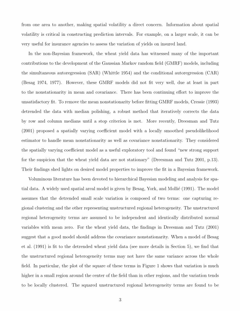
from one area to another, making spatial volatility a direct concern. Information about spatial

volatility is critical in constructing prediction intervals. For example, on a larger scale, it can be

very useful for insurance agencies to assess the variation of yields on insured land.

In the non-Bayesian framework, the wheat yield data has witnessed many of the important

contributions to the development of the Gaussian Markov random field (GMRF) models, including

the simultaneous autoregression (SAR) (Whittle 1954) and the conditional autoregression (CAR)

(Besag 1974, 1977). However, these GMRF models did not fit very well, due at least in part

to the nonstationarity in mean and covariance. There has been continuing effort to improve the

unsatisfactory fit. To remove the mean nonstationarity before fitting GMRF models, Cressie (1993)

detrended the data with median polishing, a robust method that iteratively corrects the data

by row and column medians until a stop criterion is met. More recently, Dreesman and Tutz

(2001) proposed a spatially varying coefficient model with a locally smoothed pseudolikelihood

estimator to handle mean nonstationarity as well as covariance nonstationarity. They considered

the spatially varying coefficient model as a useful exploratory tool and found “new strong support

for the suspicion that the wheat yield data are not stationary” (Dreesman and Tutz 2001, p.13).

Their findings shed lights on desired model properties to improve the fit in a Bayesian framework.

Voluminous literature has been devoted to hierarchical Bayesian modeling and analysis for spa-

tial data. A widely used spatial areal model is given by Besag, York, and Mollie (1991). The model

assumes that the detrended small scale variation is composed of two terms: one capturing re-

gional clustering and the other representing unstructured regional heterogeneity. The unstructured

regional heterogeneity terms are assumed to be independent and identically distributed normal

variables with mean zero. For the wheat yield data, the findings in Dreesman and Tutz (2001)

suggest that a good model should address the covariance nonstationarity. When a model of Besag

et al. (1991) is fit to the detrended wheat yield data (see more details in Section 5), we find that

the unstructured regional heterogeneity terms may not have the same variance across the whole

field. In particular, the plot of the square of these terms in Figure 1 shows that variation is much

higher in a small region around the center of the field than in other regions, and the variation tends

to be locally clustered. The squared unstructured regional heterogeneity terms are found to be

3

spatially correlated from an exploration analysis using both the Moran and the Geary statistics;

see more details in Section 5. This implies that the regional heterogeneity may have local clustering

in their variation, and may not be completely “unstructured”. Therefore, one way to extend Besag

et al. (1991)’s model is simply to allow the regional heterogeneity terms to have spatially varying

variance, as supported by the exploratory analysis.

In this article, we introduce a spatial stochastic volatility (SSV) component into the widely used

hierarchical spatial model of Besag et al. (1991) to capture the spatial clustering in heteroskedas-

ticity. The basic idea is adapted from the time series analog. The SSV component is a mean zero,

conditionally independent Gaussian process given a latent spatial process of the variances. To en-

sure positivity of the variance and allow spatial clustering, we use a GMRF to model the logarithm

of the latent variance. This GMRF can be intrinsic as for the spatial clustering effect in Besag

et al. (1991). With the SSV component, the new spatial model is a more intuitive alternative in

the Bayesian framework to the spatially varying coefficient model of Dreesman and Tutz (2001) by

providing posterior surfaces of the spatial heteroskedasticity as well as the spatial clustering effect.

The rest of the paper is organized as follows. In Section 2, we briefly review the traditional

model of Besag et al. (1991) and then discuss strategies to fix its limitation in handling spatial

heteroskedasticity. The proposed SSV model is introduced in Section 3. Implementation details for

Bayesian computing are discussed in Section 4. In Section 5, the classic wheat yield data (Mercer

and Hall 1911) is reanalyzed using the SSV model and the results are compared to those obtained

from the traditional model Besag et al. (1991). The SSV model is found to pick up the spatial

clustering of heteroskedasticity hidden from the existing analysis. A summary and discussion of

future research directions conclude in Section 6.

2. BESAG, YORK, AND MOLLIE’S (1991) MODEL

Consider a spatial process {Yi : i = 1, . . . , n} on a lattice D. Without loss of generality, assume

that there is no fixed effect in the sequel except an overall level µ. Fixed effects capturing the large

scale variation can be added to the model by replacing µ with X>i β for covariate vector Xi and

4

coefficient vector β. A popular formulation given by Besag et al. (1991) is:

Yi = µ + φi + εi,

φi|φj 6=i ∼ N(P

j 6=i bijφjPj 6=i bij

,σ2

φPj 6=i bij

),

εi ∼ N(0, σ2ε),

(1)

where φi is a random effect to capture the small-scale variation in region i attributable to regional

clustering, εi represents unstructured noise, bij’s are known weights with bij = bji, and σ2φ and σ2

ε

are variance parameters. It is the conditionally specified {φi}, which follows a Gaussian Markov

random field, that make model (1) a spatial model. A common choice for weight bij is 1 if site i and

site j are immediate neighbors and 0 otherwise. This choice will be used in the sequel. Note that the

specification of {φi} leaves the overall mean level of the GMRF unspecified. It can be shown that

only the pairwise differences between neighboring sites are specified (Besag and Kooperberg 1995).

The GMRF in model (1) therefore corresponds to an improper prior joint distribution of {φi};

see more discussion in Section 3. The heterogeneity effects {εi} are independent and identically

distributed normal variables. This model separates the variability of the observations into local

clustering and global heterogeneity, which can both be of scientific interest. The two-component

error decomposition can be used in more general settings, such as generalized linear models and

survival models, finding applications in a variety of fields including economics, epidemiology, and

social science, among others.

Successful as model (1) has been, it provides only limited accommodation to spatial het-

eroskedasticity, which may arise jointly with spatial autocorrelation in many spatial settings. Sim-

ilar to a spatial process, spatial heteroskedasticity itself may exhibit local clustering. That is, sites

with high volatility tend to have neighbors with high volatilities and those with low volatility tend

to have neighbors with low volatilities. Heteroskedasticity clustering occurs naturally when there

are measurement errors. If a variable is hard to measure precisely in a region, then it may be

more likely to be hard to measure in the surrounding regions. For example, the difficulty level of

measuring snow water equivalent (Cowles et al. 2002) may cluster according to the geographical

contiguity. Model (1) implicitly specifies conditional heteroskedasticity through the spatial cluster-

ing effects {φi}. It postulates that the conditional variance of φi given φj 6=i depends inversely on

5

the number of its neighbors. However, there is no spatially varying structure explicitly imposed

on the marginal variance of {φi}. The spatial heterogeneity effects {εi} are assumed to have con-

stant volatility (CV), which cannot reflect the local clustering effect of heteroskedasticity for many

environmental datasets with clustered volatility of measurement errors.

Ideas of heteroskedasticity modeling in time series are to be adapted to the spatial analog. There

are two classes of heteroskedasticity models in time series: autoregressive conditional heteroskedas-

ticity (ARCH) and stochastic volatility (SV); see survey articles, for example, by Bollerslev, Engle,

and Nelson (1994) for ARCH and Ghysels, Harvey, and Renault (1996) for SV. In an ARCH model,

the conditional variance is modeled as a deterministic function of the available information; while

in an SV model, the conditional variance is modeled as a latent stochastic process. These mod-

eling strategies may be applied to {εi} in model (1). In a spatial ARCH (SARCH) model, one

would like to assume the conditional distribution of εi given εj 6=i to be normal with mean zero and

variance a function of εj 6=i. However, the existence of the joint distribution of {εi} determined by

these assumed full conditional distributions is unknown. On the other hand, in an spatial stochas-

tic volatility model, one ends up with a hierarchical model which has been extensively studied

in the Bayesian paradigm. Assume there is a latent volatility process {σ2i } which has local clus-

tering. Given this volatility process, the conditional distribution of εi is independent N(0, σ2i ),

i = 1, . . . , n. When the SSV model for {εi} is introduced into model (1), one more layer of the

hierarchical structure is formed from the {σ2i }; see details of the revised model in Section 3.

3. SPATIAL STOCHASTIC VOLATILITY

We start by modifying the traditional model (1). Let Y = {Yi} denote the vector of observed

responses, φ = {φi} the vector of spatial clustering random effects, and ε = {εi} the vector of the

unstructured heterogeneity (often measurement errors). Conditioning on φ, Y in model (1) follows

a multivariate normal distribution N(µ + φ, σ2εI). To allow spatially varying heteroskedasticity,

we introduce a latent variance process σ2 = {σ2i }, and use it to replace the constant conditional

variance σ2ε I of Y . That is,

Y |µ, φ, σ2 ∼ N(µ + φ, diag σ2).

6

To impose a spatially smooth structure on σ2, we let σ2i = exp(µh + hi), where µh is an overall

level of the log volatility, and h = {hi} follows another CAR model in the same way as φ.

We now present the model with spatial stochastic volatility:

Yi = µ + φi + εi,

φi|φj 6=i ∼ N(P

j 6=i bijφjPj 6=i bij

,σ2

φPj 6=i bij

),

εi ∼ N(0, exp(µh + hi))

hi|hj 6=i ∼ N(P

j 6=i cijhjPj 6=i cij

,σ2

hPj 6=i cij

),

(2)

where the cij’s are pre-specified weights playing the same role for h as the bij’s do for φ in model

(1), σ2h is the variance parameter for h, and all other parameters have the same meaning as in

model (1). To make the parameters µ and µh identifiable, we add the constraints∑n

i=1 φi = 0 and∑ni=1 hi = 0, respectively. The weights {cij} can be different from {bij} in general, but in practice,

we can choose them to be the same. Model (2) distinguishes itself from model (1) by putting a

smoothly-changing spatial structure on the variance of the εi’s. When σ2h approaches zero, the

variation in h vanishes, and model (2) reduces to the constant volatility model (1). The process

{εi} in (2) can be used as an error process alone even without the presence of spatial clustering

effects φ; see Table 2 in Section 5. In a generalized linear models setup, we can replace the first

equation in (2) with

ηi = µ + φi + εi, (3)

where ηi is the linear predictor with ηi = g{E(Yi)} for link function g. However, we limit the scope

in this paper to the case of normal responses.

The incorporation of a latent spatial process h in the log volatility has the same flavor as

the spatially varying coefficient processes in the literature. For point referenced data, Gelfand

et al. (2003) viewed the regression coefficients as realizations from latent spatial processes, and

applied their method to explain housing prices. Assuncao (2003) dealt with the counterpart for

areal data. These methods offer great flexibility in regression for spatial data, providing maps of

spatially varying regression coefficients that researchers like to see. However, they do not address

the clustering of volatilities, which can be important for many applications.

7

The SSV process has a variety of characteristics that make it attractive for spatial applications.

In the case of volatility clustering, researchers may want to detect “hot spots” of volatilities, and

monitor these spots more closely in the future. This can be done naturally by the SSV model.

When prediction is of interest, the SSV model may be preferred to CV models by allowing the

variance to vary spatially. SSV can also be an approximation of a more complex model and can

pick up the effects of omitted variables. The existence of SSV would be interpreted as evidence of

misspecification, either by omitted variables or through structural change.

4. BAYESIAN IMPLEMENTATION

Model (2) can be straightforwardly implemented in a Bayesian framework using MCMC methods.

Let θ = (µ, σ2φ, µh, σ

2h)>. Let p(·) in general represent the density of its arguments. The joint

posterior distribution of interest in given by

p(θ,φ, h|y) ∝ L(µ, φ, µh, h; y)p(φ|σ2φ)p(h|σ2

h)p(µ)p(σ2φ)p(µh)p(σ2

h), (4)

where the first term L on the right-hand side is the likelihood, and the remaining terms are prior

densities. Marginal posteriors of interest can be obtained from (4) by integrating out any unwanted

parameters. For the normal case,

L(µ, φ, µh, h; y) ∝n∑

i=1

exp

{−1

2

n∑i=1

(µh + hi)

}exp

{−1

2

n∑i=1

(yi − µ− φi)2

exp(µh + hi)

}. (5)

It can be shown (e.g. Hodges, Carlin, and Fan 2003) that the improper joint distributions p(φ|σ2φ)

and p(h|σ2h) are

p(φ|σ2φ) ∝ σ

−(n−1)φ exp

{−

∑i∼j (φi − φj)

2

2σ2φ

}, (6)

and

p(h|σ2h) ∝ σ

−(n−1)h exp

{−

∑i∼j (hi − hj)

2

2σ2h

}, (7)

respectively, where i ∼ j if i and j are neighboring sites. Note that the exponents are n− 1 instead

of n, as rigorously shown by Hodges et al. (2003). Prior specification of θ completes the Bayesian

setup. For µ and µh, a flat (improper uniform) prior can be used. For variance parameters σ2φ and

σ2h, a vague but proper prior is chosen. Let IG(a, b) denote an inverse gamma distribution with

8

mean b/(a − 1). Choosing IG(aφ, bφ) and IG(ah, bh) as priors for σ2φ and σ2

h has the advantage of

being semi-conjugate in terms of their full conditionals.

MCMC algorithms for drawing samples from posterior distribution of the parameters in the CV

model (1) have become standard and are available in the widely used software BUGS (Spiegelhalter

et al. 1995). Therefore, here we only examine whether there is any extra difficulty brought by the

SSV in model (2). Reparameterize µh and h as λ = {µh + hi}. Once we have λ, µh and h can be

obtained by applying the constraint∑n

i=1 hi = 0. The full conditional of λi is

p(λi|λ−i, µ,φ, σ2h, y) ∝ p(λi|λ−i, σ

2h)p(yi|µ, φi, λi), (8)

where λ−i denotes the vector λ with λi excluded. The first term p(λi|λ−i, σ2h) is simply the density

of N(λ∗i , ν2i ), where λ∗i =

∑j∼i λj/mi and ν2

i = σ2h/mi with mi being the number of neighbors of

site i. The second term can be bounded up to a scaling constant (Kim, Shephard, and Chib 1998,

p.365),

p(yi|µ, φi, λi) ∝ exp

[−1

2λi −

(yi − µ− φi)2

2exp(−λi)

]≤ exp

[−1

2λi −

(yi − µ− φi)2

2{exp(−λ∗i )(1 + λ∗i )− λi exp(λ∗i )}

].

By completing the square of λi, the term on the right-hand side of (8) can then be shown to be

bounded, up to a scale, by the density of

N(λ∗i +

νi

2[(yi − µ− φi)

2 exp(−λ∗i )− 1], ν2i

). (9)

An accept-rejection algorithm can then be used to sample λi from its full conditional (e.g. Robert

and Casella 1999, p.49). Furthermore, the density in (8) is a log-concave density, as

∂2

∂λi

log p(λi|λ−i, µ,φ, σ2h, y) = − 1

ν2i

− (yi − µ− φi)2

2exp(−λi) < 0. (10)

Therefore, a more efficient adaptive rejection sampling (ARS) method can be used (Robert and

Casella 1999, section 2.3.3). This is within the capability of BUGS, which means that the SSV

model is easily accessible by scientists with little programming efforts.

Appropriate choice of prior distribution for the hyperparameters σ2φ and σ2

ε in the CV model

and σ2φ and σ2

h in the SSV model. For the CV model, Best et al. (1999) find that IG(0.5, 0.0005),

9

suggested by Kelsall and Wakefield (1999), may be a more reasonable prior for the variance param-

eters σ2φ and σ2

ε . On the scale of standard deviation, which is the easiest to interpret, the resulted

0.01, 0.50, and 0.99 quantiles are 0.012, 0.047, and 2.52. To get an idea of how this prior compares

to the priors originally used by Best et al. (1999), one can look at the 0.01 and 0.99 quantiles on

the scale of the standard deviation. For IG(0.1, 0.1), these quantiles are 0.251 and 4.057 × 109.

For IG(0.001, 0.001), the 0.01 quantile is 6.240 while the 0.99 quantile is beyond the numerical

precision of most softwares — for example, it is computed as infinity in R (R Development Core

Team 2005). Therefore, the IG(0.5, 0.0005) prior puts considerable greater prior mass near zero,

which is reasonable for many applications. This prior is used in the analysis of the wheat yield

data in Section 5, given that the data has sample standard deviation 0.371.

For the SSV model, the prior for σ2φ can be specified similarly as for the CV model, but care is

needed to in specifying the prior of σ2h since {hi} is on the log scale of the variance {σi}. Because

of amplification effect of log transformation around the neighborhood of zero, the log scale is very

sensitive to numbers close to zero. Clearly, the overall level µh affects the magnitude of the variation

level of {hi}. In order to make a fair prior between σφ and {σi}, one million realizations of σφ were

generated from the prior IG(0.5, 0.0005), log transformed, and then centered on the log scale. The

observed 0.01 and 0.99 quantiles of the resulted quantity is 0.028 and 7.536 in absolute value. A

convenient choice of prior for σ2h is IG(0.5, 0.005), which yields 0.01 and 0.99 quantiles on the scale

of standard deviation 0.039 and 7.979, respectively.

It would be interesting to compare the fit of the constant volatility model (1) and the SSV model

(2). A convenient model choice criterion is the Deviance Information Criterion (DIC) (Spiegelhalter

et al. 2002) defined as

DIC = D + pD,

where D is the posterior expectation of the deviance, and pD is the effective number of parameters.

The first term represents the fit of the model, and the second term measures the complexity of the

model. The effective number of parameters pD is obtained as the difference between the posterior

expected deviance and the deviance evaluated at the posterior expectations. This number is typ-

ically smaller than the actual total number of parameters with random effects included, since the

10

random effects have dependence structure. The DIC is particularly useful in comparing models

with a large number of random effects. Lower DIC implies preferred model. It has been applied

in both spatial frailty models (Banerjee, Wall, and Carlin 2003) and stochastic volatility models

in time series (Berg, Meyer, and Yu 2004), although the use of DIC is controversial for its lack of

rigorous theoretical foundation in general settings; see the discussion of Spiegelhalter et al. (2002),

for example, Smith (2002). We adopt the DIC in this article for what it is worth as an informal

model comparison tool in the data analysis in Section 5. Further investigation with other model

comparison methods would certainly be helpful.

5. WHEAT YIELD DATA REVISITED

Peculiar trends in this data have been documented in the literature (Cressie 1993, p.250), probably

due to an earlier ridge and furrow pattern of plowing on the field. Neither a linear trend nor a

periodic component was found flexible enough to capture the large-scale variation in the data.

The median-polish algorithm is a robust way to decompose the trend into an overall effect, row

effects, and column effects. It has attractive outlier-resistance properties and may yield less-biased

residuals than the mean based method. Cressie (1993) remarked that the spatial trend, or large

scale variation, must be taken into account before parameters of the small scale variation can be

interpreted. To focus on the modeling of spatial heteroskedasticity, the data used in this paper is

the median-polish residuals (Cressie 1993, Section 3.5) with spatial trend removed. The median-

polish surface of the data can be found on page 252 of Cressie (1993). The residuals {yi} from

median-polishing, shown in Figure 1, are the starting point of our analysis. They have median 0,

mean −0.012, and standard deviation 0.371.

[Figure 1 about here.]

5.1 Constant Volatility Model

The first model we fit is the widely used CV model (1) of Besag et al. (1991). The parameters of

interest are {µ, φ, σ2φ, σ

2ε}. A non-informative flat prior is chosen for µ. The prior distribution of

σ2φ and σ2

ε are both chosen to be IG(0.5, 0.0005), following the suggestion of Kelsall and Wakefield

11

(1999). Given the magnitude 0.371 of the standard deviation of {yi} this is a reasonable choice.

We ran 500,000 MCMC samples, discarded the first 100,000, and recorded every 100th of the

remaining samples, resulting in 4,000 samples for summarizing. Table 1 gives the 2.5, 50, and 97.5

posterior percentiles for the parameters µ, σφ, and σε. Since we started with the detrended residuals,

our focus here is σφ, and σε. Although these quantities give a rough idea about the decomposition of

the variation in yi’s, they are not directly comparable, since one is for the conditional specification

and the other is for the usual marginal specification (Banerjee, Carlin, and Gelfand 2004, p.164).

[Table 1 about here.]

The surface of the posterior medians of {φi}, {εi}, and {ε2i }, denoted by {φi}, {εi}, and {ε2

i },

respectively, are plotted in Figure 1. The surface of {φi} is smooth. Though it is hard to observe any

pattern in the plot of {εi}, the plot of {ε2i } does show some pattern of clustering. That is, high (low)

values of ε2i tend to have high (low) values in the surrounding vicinity, potentially contradicting the

constant volatility assumption on {εi}.

Based on 10,000 random permutations, the observed Moran and the Geary statistics have P-

values 0.9983 and 0.9974 for the εi process, and 0.0142 and 0.0134 for the ε2i process, respectively.

These tests suggest no evidence of clustering in εi’s, but strong evidence of clustering in ε2i ’s. This

motivates us to fit a stochastic volatility model (2).

5.2 Spatial Stochastic Volatility

Model (2) is now fitted, with the hope to better describe the data. Non-informative flat priors are

chosen for µ and µh. The prior distributions of the variance parameters σ2φ and σ2

h are IG(0.5, 0.0005)

and IG(0.5, 0.005), respectively.

The same number of MCMC samples are collected for parameters in the SSV model. The 2.5,

50, and 97.5 posterior percentiles for the parameters are also presented in Table 1. The posterior

median of spatial clustering effects {φi} and the posterior median of latent standard deviation {σi}

are plotted in Figure 2.

[Figure 2 about here.]

12

Compared to the spatial clustering effect in the CV model, the surface of {φi} in the SSV model

is similar. except that it is maybe slightly smoother. This is consistent with the similar posterior

median of σφ in both models, 0.394 in the CV model and 0.386 in the SSV model. A wide range

of priors for σ2h has been tried, such as IG(0.5, 0.05), IG(0.1, 0.1), and IG(1, 1), and the results in

Table 1 does not change much.

The essential utility of the SSV model is seen from the posterior median surface of {sigmai},

which closely resembles the surface shape of the {ε2i } in Figure 1, picking up the spatial clustering

in volatility. Clearly from Figure 2, the volatility in the north-east corner is much lower than that

in the center and the north-west corner of the field. We can summarize the posterior median of the

spatially varying standard deviation {σi} from the MCMC samples. The median of these medians

is 0.209 in the SSV model, compared to median 0.242 in the CV model. Their range is from 0.115

to 0.486, thus differing by a factor of 4.2.

It is also worth noting from Figure 1 and Figure 2 that the clustering patterns of the spatial

effects {φi} and the stochastic volatility {σ2i } are generally different. A high value in φi does not

necessarily imply high volatility, since its neighbor may also have high values of φi. It is possible

that high volatility appears at positions with φi’s low in magnitude. Actually, a closer investigation

of the center of the field, where the volatility is the highest, reveals that wheat yield residuals in

this area are not high in magnitude but are very different from one plot to another, implying high

volatility.

To compare the error decomposition of the two models, Figure 3 plots the posterior median

of {µ + φi} from the CV model against that from SSV model, together with the 45 degree line.

Most of the points lie about the 45 degree line except for some points at the tails. The range is

(−0.648, 0.914) from the CV model and (−0.721, 0.729) from the SSV model, suggesting that the

SSV model is pushing variations of a large residual from the spatial clustering effect {φi} to the

spatial heteroskedastic effect {εi}. Figure 3 also plots the posterior median spatial heteroskedastic

effect {εi} and the posterior median latent variance {σ2i } in the SSV model. It is clear that the

SSV model provides larger variance for larger errors.

[Figure 3 about here.]

13

Table 2 compares the CV and SSV models in terms of the DIC and effective number of pa-

rameters pD. It is worth noting that the deviances are computed only up to an additive constant.

Therefore the DIC can be negative and can only be compared across models under the same distri-

butional assumption. As seen in Figure 3 (b), most sites have relatively low volatilities except for

those clustered “hot spots”. Therefore, putting a structure on the volatility via SSV improves the

fit significantly. The CV model is soundly beaten by the SSV model in terms of their DIC values.

Both models have effective number of parameters pD much smaller than their nominal parameter

counts, which would include 500 and 1000 random effects in the CV and SSV models, respectively.

The more complicated SSV model has even smaller pD than the simpler CV model. This is, how-

ever, not unusual; see for example the analysis of Scottland lip cancer data in Spiegelhalter et al.

(2002).

[Table 2 about here.]

To illustrate that the spatial volatility process εi can be used alone in a model without the

spatial clustering effects φi, we also fit a model of the form

Yi = µ + εi, (11)

denoted as SSV0 in Table 2, where {εi} is the same as those in the SSV model (2). This model

ignores the spatial clustering in the mean, and does not fit the data as well as the CV model (1)

from the DIC comparison.

Table 2 also presents DIC results for two other competitive models suggested by a referee. The

CV-t model is the same as the CV model except that the conditional distribution of Yi given φi is

t with degrees of freedom df , scaled by σε. The SV-iid model is the same as the SSV model except

that the prior distribution of {hi} is independent N(0, σ2h), without any spatial varying structure.

These two models both allow large residuals. In terms of DIC, the CV-t model fits better than the

CV model, and the SV-iid model fits better than the SSV model. During the experimental fitting

process, the DIC of the SSV model and SV-iid model are not robust to prior changes, although the

value of pD are. Even though the SV-iid model always has smaller DIC than the SSV model under

14

all the experimented priors in this example, the SSV model may still be preferred, as illustrated

below, in situations such as prediction for its spatially varying nature in the latent variance {σ2i }.

As a pilot study to compare the predicting capability of the CV model and the SSV model,

Table 3 presents the leaving-one-out 95% prediction intervals of some selected points in the plot.

Three sites in row 12 and three sites in column 18 are chosen, representing high volatility and low

volatility regions, respectively. For each site, the observed value is replaced with missing value

and then the two models are fitted. The reported prediction intervals are obtained from the 4,000

posterior samples. One observe that center of the prediction interval from the two models are very

close. However, the standard deviation of the prediction at all sites are about the same from the

CV model, but vary noticeably from the SSV model. Consequently, compared to the CV model,

the prediction intervals from the SSV model is wider for larger residuals and narrower for smaller

residuals. A full comparison of the predicting capability at all 500 sites with this leaving-one-out

procedure is beyond the scope of this paper but is of great interest in future studies.

[Table 3 about here.]

6. DISCUSSION

In this paper we have introduced a SSV component into the widely used model of Besag et al. (1991).

The SSV component allows the regional heterogeneity effects to have variance clustering spatially.

The model is applied to the well-known wheat yield data and compared with the traditional constant

volatility model. Volatility clustering is found to be present in the data. The SSV model is easy to

implement and can be useful in a wide range of spatial applications, particularly when the volatility

of measurement errors clusters.

As pointed by a referee, the identification issue of the SSV model needs to addressed. That is,

given a large residual ei = φi + εi, how do we know if it is due to a large spatial clustering effect

φi or spatial heteroskedastic effect εi? Actually, this question applies not only to the SSV model

but also to the CV model. The data Yi cannot inform about φi or εi, but only about their sum

ei. Therefore, φi and εi are Bayesian unidentifiable. However, Bayesian learning, that is, prior to

posterior movement, is still feasible (Banerjee et al. 2004, p.165). When the true model has a SSV

15

component, a large residual ei is likely to be surrounded by residuals with large magnitude, but

not necessarily of the same sign. If a large residual is surrounded by large residuals of the same

sign, then it may be more likely to be picked up by the spatial clustering effect φi. It is the spatial

structure imposed by the priors of {φi} and {εi} that makes “borrowing strength from neighbors”

possible. Vague, fair and proper priors for the variance parameters σ2φ and σ2

h are important.

Further investigation along this line may be worthwhile.

Several directions of extending the SSV model are immediate. We demonstrated the SSV model

assuming that the large scale variation has been removed. With the overall level µ in model (2)

replaced by a linear predictor X>i β, the algorithm in Section 4 can be easily adapted to include

the unknown parameter vector β in the constructed linear structure. Although we focused on a

lattice setup, the essentials of the SSV can be carried over to irregularly spaced data, in which case,

weight matrices must be appropriately chosen, similar to what Pettitt, Weir, and Hart (2002) did

for a CAR model. The SSV can also be used as a random effect which replaces the commonly used

homoskedastic term in a model for non-normal data, for example, count data for disease mapping

as Haran, Hodges, and Carlin (2003) did in a generalized linear model setting.

The other class of models for volatility in time series, the ARCH model, is promising to provide

an alternative way for volatility clustering. Bera and Simlai (2003) got the specification of a spatial

ARCH model as a byproduct of an information matrix (IM) test. The error term is a replacement

for the i.i.d. error in a Simultaneous Autoregressive (SAR) model, which does not have much

overlap with the general hierarchical model (1).

REFERENCES

Assuncao, R. (2003), “Space varying coefficient models for small area data,” Environmetrics, 14,

453–473.

Banerjee, S., Carlin, B. P., and Gelfand, A. E. (2004), Hierarchical modeling and analysis for spatial

data, Chapman & Hall / CRC.

Banerjee, S., Wall, M. M., and Carlin, B. P. (2003), “Frailty Modeling for Spatially Correlated

16

Survival Data, with Application to Infant Mortality in Minnesota,” Biostatistics (Oxford), 4,

123–142.

Bera, A. K. and Simlai, P. (2003), “Testing for spatial dependence and a formulation of spatial

ARCH (SARCH) model with applications,” Thirteenth Annual Meeting of the Midwest Econo-

metrics Group.

Berg, A., Meyer, R., and Yu, J. (2004), “Deviance Information Criterion for Comparing Stochastic

Volatility Models,” Journal of Business & Economic Statistics, 22, 107–120.

Besag, J. (1974), “Spatial interaction and the statistical analysis of lattice systems (with discus-

sion),” Journal of the Royal Statistical Society, Series B, Methodological, 36, 192–236.

— (1977), “Errors-in-variables Estimation for Gaussian Lattice Schemes,” Journal of the Royal

Statistical Society, Series B: Methodological, 39, 73–78.

Besag, J. and Kooperberg, C. (1995), “On conditional and intrinsic autoregressions,” Biometrika,

82, 733–746.

Besag, J., York, J., and Mollie, A. (1991), “Bayesian image restoration, with two applications in

spatial statistics (Disc: p21-59),” Annals of the Institute of Statistical Mathematics, 43, 1–20.

Best, N. G., Arnold, R. A., Thomas, A., Waller, L. A., and Conlon, E. M. (1999), “Bayesian Models

for Spatially Correlated Disease and Exposure Data,” in Bayesian Statistics 6 – Proceedings of

the Sixth Valencia International Meeting, eds. Bernardo, J. M., Berger, J. O., Dawid, A. P., and

Smith, A., Clarendon Press [Oxford University Press], pp. 131–156.

Bollerslev, T., Engle, R., and Nelson, D. (1994), “ARCH models,” in The Handbook of Economet-

rics, eds. Engle, R. and McFadden, D., Amsterdam: North-Holland, pp. 2959–3038.

Cowles, M. K. and Zimmerman, D. L. (2003), “A Bayesian space-time analysis of acid depo-

sition data combined from two monitoring networks,” Journal of Geophysical Research, 108,

doi:10.1029/2003JD004001.

17

Cowles, M. K., Zimmerman, D. L., Christ, A., and McGinnis, D. L. (2002), “Combining snow

water equivalent data from multiple sources to estimate spatio-temporal trends and compare

measurement systems,” Journal of Agricultural, Biological, and Environmental Statistics, 7, 536–

557.

Cressie, N. A. C. (1993), Statistics for spatial data, John Wiley & Sons.

Dreesman, J. M. and Tutz, G. (2001), “Non-stationary Conditional Models for Spatial Data Based

on Varying Coefficients,” Journal of the Royal Statistical Society, Series D: The Statistician, 50,

1–15.

Gelfand, A. E., Kim, H.-J., Sirmans, C. F., and Banerjee, S. (2003), “Spatial Modeling with

Spatially Varying Coefficient Processes,” Journal of the American Statistical Association, 98,

387–396.

Ghysels, E., Harvey, A., and Renault, E. (1996), “Stochastic volatility,” in Statistical Methods in

Finance, eds. C.R., R. and G.S., M., Amsterdam: North-Holland, pp. 119–191.

Haran, M., Hodges, J. S., and Carlin, B. P. (2003), “Accelerating computation in Markov Random

Fields Models for Spatial Data via Structured MCMC,” Journal of Computational and Graphical

Statistics, 12, 249–264.

Hodges, J. S., Carlin, B. P., and Fan, Q. (2003), “On the precision of the conditional autoregressive

prior in spatial models,” Biometrics, 59, 317–322.

Kelegian, H. H. and Robinson, D. P. (1998), “A suggested test for spatial autocorrelation and/or

heteroskedasticity and corresponding Monte Carlo results,” Regional Science and Urban Eco-

nomics, 28, 389–417.

Kelsall, J. E. and Wakefield, J. C. (1999), “Comment on “Bayesian Models for Spatially Correlated

Disease and Exposure Data”,” in Bayesian Statistics 6 – Proceedings of the Sixth Valencia Inter-

national Meeting, eds. Bernardo, J. M., Berger, J. O., Dawid, A. P., and Smith, A., Clarendon

Press [Oxford University Press], p. 151.

18

Kim, S., Shephard, N., and Chib, S. (1998), “Stochastic Volatility: Likelihood Inference and Com-

parison with ARCH Models,” Review of Economic Studies, 65, 361–393.

Mercer, W. B. and Hall, A. D. (1911), “The experimental error of field trials,” Journal of Agricul-

tural Science (Cambridge), 4, 107–132.

Pettitt, A. N., Weir, I. S., and Hart, A. G. (2002), “A conditional autoregressive Gaussian process

for irregularly spaced multivariate data with application to modelling large sets of binary data,”

Statistics and Computing, 12, 353–367.

R Development Core Team (2005), R: A language and environment for statistical computing, R

Foundation for Statistical Computing, Vienna, Austria, ISBN 3-900051-07-0.

Robert, C. P. and Casella, G. (1999), Monte Carlo Statistical Methods, Springer-Verlag Inc.

Smith, J. (2002), “Comment on “Bayesian Measures of Model Complexity and Fit” (Pkg: P583-

639),” Journal of the Royal Statistical Society, Series B: Statistical Methodology, 64, 619–620.

Spiegelhalter, D. J., Best, N. G., Carlin, B. P., and van der Linde, A. (2002), “Bayesian Measures

of Model Complexity and Fit (Pkg: P583-639),” Journal of the Royal Statistical Society, Series

B: Statistical Methodology, 64, 583–616.

Spiegelhalter, D. J., Thomas, A., Best, N. G., and Gilks, W. R. (1995), “BUGS: Bayesian inference

using Gibbs sampling, Version 0.50,” Technical report, Medical Research Council Biostatistics

Unit, Institute of Public Health, Cambridge University.

Whittle, P. (1954), “On statitionary processes in the plane,” Biometrika, 41, 434–449.

19

West−East

5

10

1520

25

North−S

outh

5

10

15

20−1.0−0.50.00.51.01.5

(a) wheat yield residual {yi} from median−polish

West−East

5

10

1520

25

North−S

outh

5

10

15

20−1.0−0.50.00.51.01.5

(b) posterior median of spatial effect {φi}

West−East

5

10

1520

25

North−S

outh

5

10

15

20−1.0−0.50.00.51.01.5

(c) posterior median of residual {εi}

West−East

5

10

1520

25

North−S

outh

5

10

15

200.0

0.2

0.4

0.6

(d) squared residual {εi2}

Figure 1: Three–dimensional perspective of the wheat yield data and results from the constantvolatility model of Besag, York, and Mollie (1991), yi = µ + φi + εi: (a) Wheat yield residual {yi}from Median-Polish; (b) Posterior median of the spatial clustering effect {φi}; (c) Posterior medianof the spatial heterogeneity effect {εi}; (d) Squared posterior median of the spatial heterogeneityeffect {ε2

i }.

20

West−East

5

10

1520

25

North−S

outh

5

10

15

20−1.0−0.50.00.51.01.5

(a) posterior median of spatial effect {φi}

West−East

5

10

1520

25

North−S

outh

5

10

15

20

0.20.3

0.4

(b) posterior median of standard deviation {σi}

Figure 2: Three–dimensional perspective of results from the stochastic volatility model: (a) Pos-terior median of the spatial clustering effects {φi}; (b) Posterior median of stochastic volatility{σi}.

●

●

●

●

●

●●

●

●

●●

●

●

●

●

●

●●

●●

●●

●

●

●

●

●●

●

●●

●

●

●

●

●

●

●

●

●

●●

●●

●

●●

●

●

●

●●

●

●

●

●

●

●●

●

●

●●

●

●

●

●

●

●

●●●

●●●●●

●

●

●

●

●

●

●

●●

●

●

●

●

●

●

●

●●

●

●

●●

●●

●

●

●●

●●

●●

●●

●●

●

●

●

●

●

●

●

●

●

●●

●

●

●

●●

●

●

●

●

●

●

●

●

●●

●●●

●

●

●●

●

●

●

●

●●

●

●

●●●

●

●●

●

●

●

●

●

●

●

●●

●●

●●

●

●

●●

●

●

●

●

●

●

●

●

●

●●

●

●●

●

●●

●

●●

●

●●●

●

●

●

●

●

●●

●

●

●●

●●

●

●

●

●●

●

●●

●

●●

●

●

●●

●

●

●

●●

●

●

●

●

●●

●

●

●

●

●

●

●

●●

●

●●●

●

●

●

●

●

●●

●●

●

●

●●

●●

●

●●●

●

●

●●

●●

●

●

●●

●

●

●●

●●

●

●●

●

●

●

●

●●●

●

●●

●

●

●

●

●

●

●

●

●

●

●

●●●

●

●

●

●

●

●

●●

●

●

●

●

●●

●

●●

●

●●

●●

●

●

●

●

●

●

●

●

●●

●

●●

●

●

●●

●

●

●

●●

●

●●●

●

●

●

●

●●

●

●

●

●●

●●

●

●

●

●

●

●●●

●●

●

●

●●

●●

●

●●●●

●●

●

●

●

●●

●

●

●

●●

●

●●

●

●

●

●

●

●●

●

●

●

●

●

●

●

●

●

●

●●●

●

●

●

●●

●

●●

●

●

●●

●

●

●

●●●●

●●

●

●●

●

●

●

●

●

●●

●

●●

●

●

●

●

●

●

●

●

●

●

●

●●

●

●

●

●

●

●●

●

●●

●

●

●

●

●

●

●

●

●

●

●

−0.5 0.0 0.5

−0.

50.

00.

5

(a) spatial clustering effect from two models{µ + φi} from CV model

{µ+

φ i}

from

SV

mod

el

● ●●●

●●● ●●●

●

●●

●

●

●

●

●

●●

●●●●

●●●●

● ●●

●

● ●

●●

●

●● ●●● ●● ●

● ●●●●●

● ●●●●● ●

●●

●

●●●

● ●● ●●●●●●

●●

●

●

●

● ●

●

●

●●●●● ●● ●●● ●

●●

●

●

●

●

●

●

●

●

● ●●●

●● ●● ●●●●

●

●●

● ●

●● ●●● ●

●

●●●●

●●●● ●

●●

●●

●●

●

●

●●

●

●

●

●

●●●

● ●● ●●

●●

●●

●

●

●

●●●●

●●

●●●● ●●●● ●

●●

●

● ●

● ●●●

●● ●●●● ●●●●●

●●● ●●

● ●●

●

● ●●

●

●●●● ●● ●

● ●●

●● ●●

●

●●

●

●

●

●●●

●●●

●

●●

●●

●●

●● ●

●

●

●

●

●●●

●●●● ●●

●●

●●● ●●

●

●

●

●

●

●● ●● ●

●

●●●

●●● ●●

●

●

●

●

●

●●

●● ●●●●●●

●

● ●

●

●●●

●

●

●

●●●●●

●●●●

● ●● ●●

● ● ●●● ●

●●●●●

● ●● ●● ● ● ●●● ●●●● ●

●●● ●●● ●

●●● ●● ●●●● ● ●●●●●

●● ●● ●

● ●●●●

● ●● ●● ●●●●

●●●●●●

●● ●●

●

●●

●●●●●●

●●●

●●●●

●●●

●●

●

●

●●

●●●

●●●

●●●●●

●●

●●●

●●

●●

●

●●● ●

●● ●● ●●

●

●●●●

●

●

●●●

●

● ●●●●● ●●●

●●

●●●

●

● ●●

●

●

●●

●●● ●●●●

−0.5 0.0 0.5 1.0

0.05

0.10

0.15

0.20

(b) spatially varying variance in errorposterior residual {εi}

post

erio

r va

rianc

e {σ

i2 }

Figure 3: Diagnostic plot of the SSV model: (a) Comparison of the posterior median of spatialclustering effects, {µ + φi}, from CV and SSV, the solid line being the 45 degree line; (b) Posteriormedian of spatial heterogeneity effect {εi} and their variance {σ2

i } in the SSV model.

21

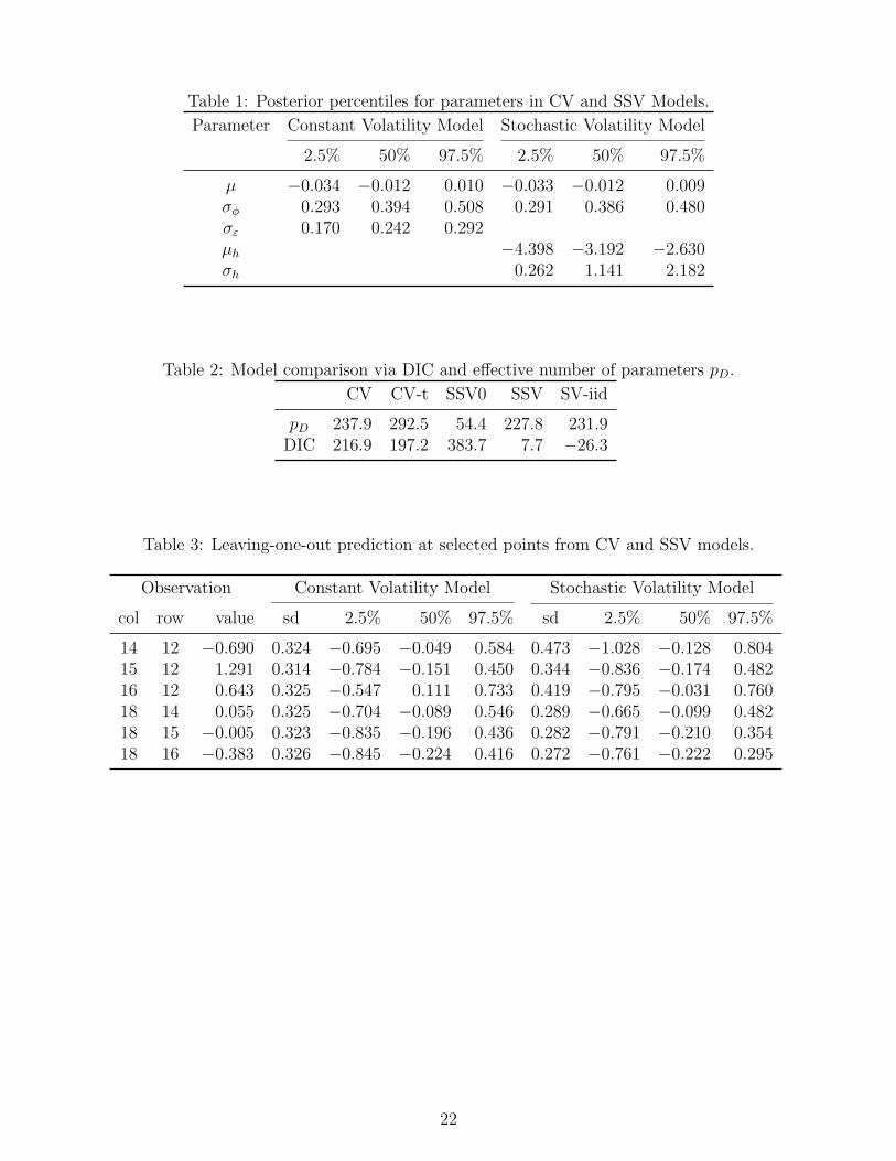
Table 1: Posterior percentiles for parameters in CV and SSV Models.

Parameter Constant Volatility Model Stochastic Volatility Model

2.5% 50% 97.5% 2.5% 50% 97.5%

µ −0.034 −0.012 0.010 −0.033 −0.012 0.009σφ 0.293 0.394 0.508 0.291 0.386 0.480σε 0.170 0.242 0.292µh −4.398 −3.192 −2.630σh 0.262 1.141 2.182

Table 2: Model comparison via DIC and effective number of parameters pD.

CV CV-t SSV0 SSV SV-iid

pD 237.9 292.5 54.4 227.8 231.9DIC 216.9 197.2 383.7 7.7 −26.3

Table 3: Leaving-one-out prediction at selected points from CV and SSV models.

Observation Constant Volatility Model Stochastic Volatility Model

col row value sd 2.5% 50% 97.5% sd 2.5% 50% 97.5%

14 12 −0.690 0.324 −0.695 −0.049 0.584 0.473 −1.028 −0.128 0.80415 12 1.291 0.314 −0.784 −0.151 0.450 0.344 −0.836 −0.174 0.48216 12 0.643 0.325 −0.547 0.111 0.733 0.419 −0.795 −0.031 0.76018 14 0.055 0.325 −0.704 −0.089 0.546 0.289 −0.665 −0.099 0.48218 15 −0.005 0.323 −0.835 −0.196 0.436 0.282 −0.791 −0.210 0.35418 16 −0.383 0.326 −0.845 −0.224 0.416 0.272 −0.761 −0.222 0.295

22