large vector autoregressions with stochastic volatility ... · large vector autoregressions with...
TRANSCRIPT
Large Vector Autoregressions with Stochastic Volatilityand Flexible Priors
Andrea Carriero1, Todd Clark2, and Massimiliano Marcellino3
1Queen Mary, University of London
2Federal Reserve Bank of Cleveland
3Bocconi University and CEPR
June 2016
Todd Clark (FRBC) Large VARs June 2016 1 / 41
Introduction
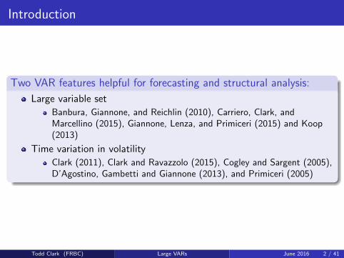
Two VAR features helpful for forecasting and structural analysis:
Large variable set
Banbura, Giannone, and Reichlin (2010), Carriero, Clark, andMarcellino (2015), Giannone, Lenza, and Primiceri (2015) and Koop(2013)
Time variation in volatility
Clark (2011), Clark and Ravazzolo (2015), Cogley and Sargent (2005),D’Agostino, Gambetti and Giannone (2013), and Primiceri (2005)
Todd Clark (FRBC) Large VARs June 2016 2 / 41
Introduction
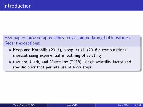
Few papers provide approaches for accommodating both features.Recent exceptions:
Koop and Korobilis (2013), Koop, et al. (2016): computationalshortcut using exponential smoothing of volatility
Carriero, Clark, and Marcellino (2016): single volatility factor andspecific prior that permits use of N-W steps
Todd Clark (FRBC) Large VARs June 2016 3 / 41

Introduction
Allowing large VARs with homoskedasticity requires symmetry oflikelihood and prior.
Homoskedastic VARs: SUR models w/ the same regressors in eachequation
Symmetry across equations Ñ likelihood has a Kronecker structure ÑOLS estimation equation by equation
With homoskedasticity, large BVARs require a specific prior structure,of conjugate N-W:
The coefficients of each equation feature the same prior variancematrix (up to a constant of proportionality).Priors are correlated across equations, with a correlation structureproportional to Σ.
Todd Clark (FRBC) Large VARs June 2016 4 / 41
Introduction
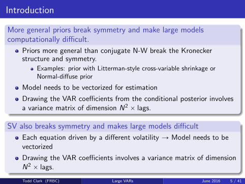
More general priors break symmetry and make large modelscomputationally difficult.
Priors more general than conjugate N-W break the Kroneckerstructure and symmetry.
Examples: prior with Litterman-style cross-variable shrinkage orNormal-diffuse prior
Model needs to be vectorized for estimation
Drawing the VAR coefficients from the conditional posterior involvesa variance matrix of dimension N2 ˆ lags.
SV also breaks symmetry and makes large models difficult
Each equation driven by a different volatility Ñ Model needs to bevectorized
Drawing the VAR coefficients involves a variance matrix of dimensionN2 ˆ lags.
Todd Clark (FRBC) Large VARs June 2016 5 / 41
Introduction
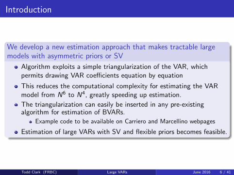
We develop a new estimation approach that makes tractable largemodels with asymmetric priors or SV
Algorithm exploits a simple triangularization of the VAR, whichpermits drawing VAR coefficients equation by equation
This reduces the computational complexity for estimating the VARmodel from N6 to N4, greatly speeding up estimation.
The triangularization can easily be inserted in any pre-existingalgorithm for estimation of BVARs.
Example code to be available on Carriero and Marcellino webpages
Estimation of large VARs with SV and flexible priors becomes feasible.
Todd Clark (FRBC) Large VARs June 2016 6 / 41
Introduction
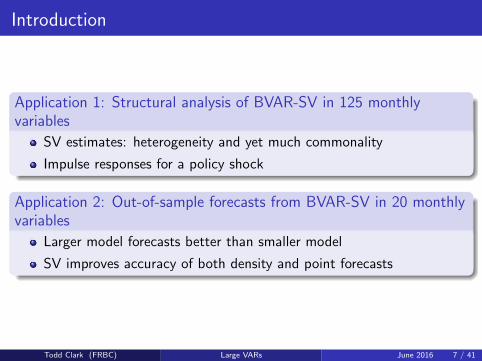
Application 1: Structural analysis of BVAR-SV in 125 monthlyvariables
SV estimates: heterogeneity and yet much commonality
Impulse responses for a policy shock
Application 2: Out-of-sample forecasts from BVAR-SV in 20 monthlyvariables
Larger model forecasts better than smaller model
SV improves accuracy of both density and point forecasts
Todd Clark (FRBC) Large VARs June 2016 7 / 41
Outline
1 BVAR-SV specification and impediments to large models
2 Our estimation method for large BVARs
3 Application 1: Structural analysis with large BVAR-SV
4 Application 2: Out-of-sample forecasting
5 Conclusions
Todd Clark (FRBC) Large VARs June 2016 8 / 41
BVAR-SV Model
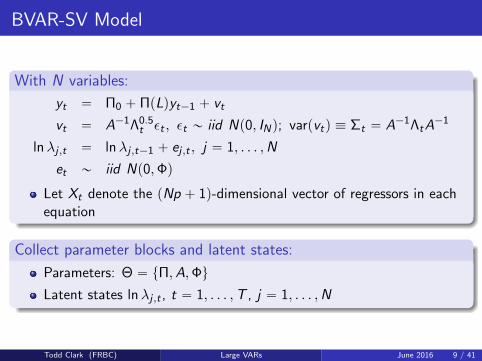
With N variables:
yt “ Π0 ` ΠpLqyt´1 ` vt
vt “ A´1Λ0.5t εt , εt „ iid Np0, INq; varpvtq ” Σt “ A´1ΛtA
´1
lnλj ,t “ lnλj ,t´1 ` ej ,t , j “ 1, . . . ,N
et „ iid Np0,Φq
Let Xt denote the pNp ` 1q-dimensional vector of regressors in eachequation
Collect parameter blocks and latent states:
Parameters: Θ “ tΠ,A,Φu
Latent states lnλj ,t , t “ 1, . . . ,T , j “ 1, . . . ,N
Todd Clark (FRBC) Large VARs June 2016 9 / 41
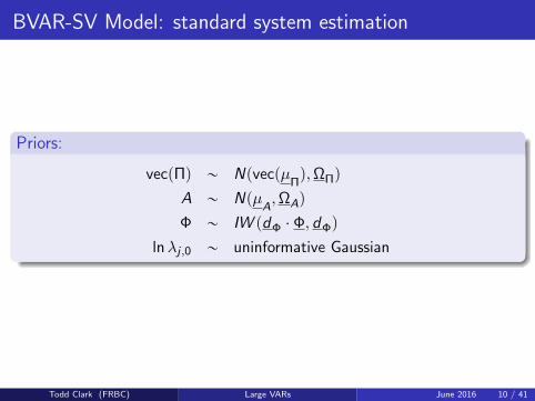
BVAR-SV Model: standard system estimation
Priors:
vecpΠq „ NpvecpµΠq,ΩΠq
A „ NpµA,ΩAq
Φ „ IW pdΦ ¨ Φ, dΦq
lnλj ,0 „ uninformative Gaussian
Todd Clark (FRBC) Large VARs June 2016 10 / 41
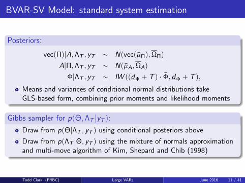
BVAR-SV Model: standard system estimation
Posteriors:
vecpΠq|A,ΛT , yT „ NpvecpµΠq,ΩΠq
A|Π,ΛT , yT „ NpµA,ΩAq
Φ|ΛT , yT „ IW ppdΦ ` T q ¨ Φ, dΦ ` T q,
Means and variances of conditional normal distributions takeGLS-based form, combining prior moments and likelihood moments
Gibbs sampler for ppΘ,ΛT |yT q:
Draw from ppΘ|ΛT , yT q using conditional posteriors above
Draw from ppΛT |Θ, yT q using the mixture of normals approximationand multi-move algorithm of Kim, Shepard and Chib (1998)
Todd Clark (FRBC) Large VARs June 2016 11 / 41

BVAR-SV Model: impediments to standard systemestimation with a large model
Sampling the VAR coefficients involves drawinga NpNp ` 1q´dimensional vector rand, and computing
vecpΠmq “ ΩΠ
#
vec
˜
Tÿ
t“1
Xty1tΣ´1t
¸
` Ω´1Π vecpµ
Πq
+
`cholpΩΠqˆrand
(1)This calculation requires: i) computing ΩΠ by inverting
Ω´1Π “ Ω´1
Π `
Tÿ
t“1
pΣ´1t b XtX
1tq;
ii) computing its Cholesky factor cholpΩΠq; iii) multiplying thematrices obtained in i) and ii) by the vector in the curly brackets of(1) and the vector rand, respectively.Each operation requires OpN6q elementary operations, making thetotal computational complexity to draw Πm equal 4ˆ OpN6q.
Todd Clark (FRBC) Large VARs June 2016 12 / 41
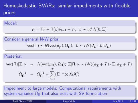
Homoskedastic BVARs: similar impediments with flexiblepriors
Model:
yt “ Π0 ` ΠpLqyt´1 ` vt , vt „ iid Np0,Σq
Consider a general N-W prior:
vecpΠq „ NpvecpµΠq,ΩΠq; Σ „ IW pdΣ ¨ Σ, dΣq
Posterior:
vecpΠq|Σ, y „ NpvecpµΠq,ΩΠq; Σ|Π, y „ IW ppdΣ ` T q ¨ Σ, dΣ ` T q
Ω´1Π “ Ω´1
Π `
Tÿ
t“1
pΣ´1 b XtX1tq
Impediment to large models: Computational requirements withsystem variance ΩΠ that also exist with SV formulation
Todd Clark (FRBC) Large VARs June 2016 13 / 41
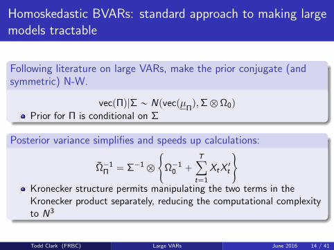
Homoskedastic BVARs: standard approach to making largemodels tractable
Following literature on large VARs, make the prior conjugate (andsymmetric) N-W.
vecpΠq|Σ „ NpvecpµΠq,Σb Ω0q
Prior for Π is conditional on Σ
Posterior variance simplifies and speeds up calculations:
Ω´1Π “ Σ´1 b
#
Ω´10 `
Tÿ
t“1
XtX1t
+
Kronecker structure permits manipulating the two terms in theKronecker product separately, reducing the computational complexityto N3
Todd Clark (FRBC) Large VARs June 2016 14 / 41

Homoskedastic BVARs: standard approach to making largemodels tractable
The conjugate (and symmetric) N-W form comes with someunappealing restrictions.
Issues discussed by Rothenberg (1963), Zellner (1973), Kadiyala andKarlsson (1993, 1997), and Sims and Zha (1998)
Rules out asymmetry in the prior across equations; coefficients ofeach equation feature the same prior variance matrix Ω0
Rules out one aspect of the Litterman (1986) prior: extra shrinkageon “other” lags vs. “own” lags
Σb Ω0 implies prior beliefs correlated across the equations of thereduced form VAR
Sims and Zha (1998) specify a prior featuring independence among thestructural equations, but does not achieve computational gains for anasymmetric prior on the reduced form.
Todd Clark (FRBC) Large VARs June 2016 15 / 41
Our estimation method for large VARs
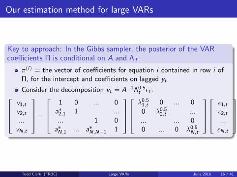
Key to approach: In the Gibbs sampler, the posterior of the VARcoefficients Π is conditional on A and ΛT .
πpiq = the vector of coefficients for equation i contained in row i ofΠ, for the intercept and coefficients on lagged yt
Consider the decomposition vt “ A´1Λ0.5t εt :
»
—
—
–
v1,t
v2,t
...vN,t
fi
ffi
ffi
fl
“
»
—
—
–
1 0 ... 0a˚2,1 1 ...
... 1 0a˚N,1 ... a˚N,N´1 1
fi
ffi
ffi
fl
»
—
—
–
λ0.51,t 0 ... 0
0 λ0.52,t ...
... ... 00 ... 0 λ0.5
N,t
fi
ffi
ffi
fl
»
—
—
–
ε1,t
ε2,t
...εN,t
fi
ffi
ffi
fl
,
Todd Clark (FRBC) Large VARs June 2016 16 / 41
Our estimation method for large VARs
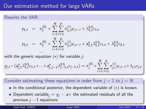
Rewrite the VAR:
y1,t “ πp0q1 `
Nÿ
i“1
pÿ
l“1
πpiq1,l yi ,t´l ` λ
0.51,t ε1,t
y2,t “ πp0q2 `
Nÿ
i“1
pÿ
l“1
πpiq2,l yi ,t´l ` a˚2,1λ
0.51,t ε1,t ` λ
0.52,t ε2,t
...with the generic equation p˚q for variable j :
yj ,t´pa˚j ,1λ
0.51,t ε1,t`...`a˚j ,,j´1λ
0.5j´1,tεj´1,tq “ π
p0qj `
Nÿ
i“1
pÿ
l“1
πpiqj ,l yi ,t´l`λj ,tεj ,t
Consider estimating these equations in order from j “ 1 to j “ N
In the conditional posterior, the dependent variable of p˚q is known.
Dependent variablej = yj ´ aˆ the estimated residuals of all theprevious j ´ 1 equations.
Todd Clark (FRBC) Large VARs June 2016 17 / 41
Our estimation method for large VARs
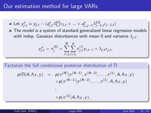
Let y˚j ,t ” yj ,t ´ pa˚j ,1λ
0.51,t ε1,t ` ...` a˚j ,,j´1λ
0.5j´1,tεj´1,tq
The model is a system of standard generalized linear regression modelswith indep. Gaussian disturbances with mean 0 and variance λj ,t :
y˚j ,t “ πp0qj `
Nÿ
i“1
pÿ
l“1
πpiqj ,l yi ,t´l ` λj ,tεj ,t ,
Factorize the full conditional posterior distribution of Π:
ppΠ|A,ΛT , yq “ ppπpNq|πpN´1q, πpN´2q, . . . , πp1q,A,ΛT , yq
ˆppπpN´1q|πpN´2q, . . . , πp1q,A,ΛT , yq...
ˆppπp1q|A,ΛT , yq,
Todd Clark (FRBC) Large VARs June 2016 18 / 41
Our estimation method for large VARs
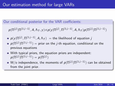
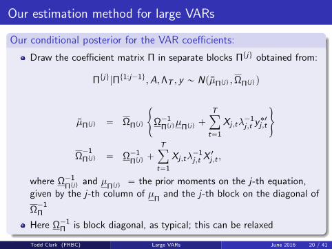
Our conditional posterior for the VAR coefficients:
ppΠtju|Πt1:j´1u,A,ΛT , yq9ppy |Πtju,Πt1:j´1u,A,ΛT qppΠ
tju|Πt1:j´1uq
ppy |Πtju,Πt1:j´1u,A,ΛT q “ the likelihood of equation j
ppΠtju|Πt1:j´1uq “ prior on the j-th equation, conditional on theprevious equations
With typical priors, the equation priors are independent:ppΠtju|Πt1:j´1uq “ ppΠtjuq
W/o independence, the moments of ppΠtju|Πt1:j´1uq can be obtainedfrom the joint prior.
Todd Clark (FRBC) Large VARs June 2016 19 / 41
Our estimation method for large VARs
Our conditional posterior for the VAR coefficients:
Draw the coefficient matrix Π in separate blocks Πtju obtained from:
Πtju|Πt1:j´1u,A,ΛT , y „ NpµΠtju ,ΩΠtjuq
µΠtju “ ΩΠtju
#
Ω´1ΠtjuµΠtju `
Tÿ
t“1
Xj ,tλ´1j ,t y
˚1j ,t
+
Ω´1Πtju “ Ω´1
Πtju `
Tÿ
t“1
Xj ,tλ´1j ,t X
1j ,t ,
where Ω´1Πtju and µ
Πtju “ the prior moments on the j-th equation,given by the j-th column of µ
Πand the j-th block on the diagonal of
Ω´1Π
Here Ω´1Π is block diagonal, as typical; this can be relaxed
Todd Clark (FRBC) Large VARs June 2016 20 / 41

Our estimation method for large VARs
Computational costs (not much):
Although we break the conditional posterior for Π into pieces, we arestill drawing from the conditional posterior for Π.
Our triangularization approach produces draws numerically identicalto those that would be obtained using system-wide estimation.
For the VAR coefficients, the ordering of variables does not matter.
Existing BVAR and BVAR-SV code can easily be modified to draw Πwith the triangularized system.
Todd Clark (FRBC) Large VARs June 2016 21 / 41
Our estimation method for large VARs
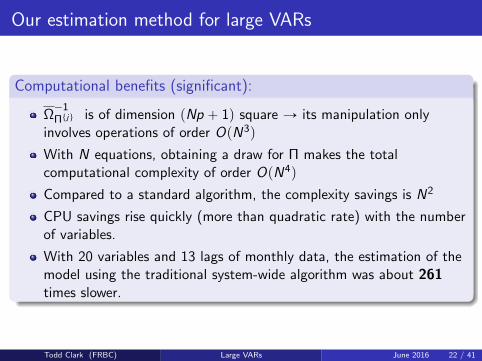
Computational benefits (significant):
Ω´1Πtju is of dimension pNp ` 1q square Ñ its manipulation only
involves operations of order OpN3q
With N equations, obtaining a draw for Π makes the totalcomputational complexity of order OpN4q
Compared to a standard algorithm, the complexity savings is N2
CPU savings rise quickly (more than quadratic rate) with the numberof variables.
With 20 variables and 13 lags of monthly data, the estimation of themodel using the traditional system-wide algorithm was about 261times slower.
Todd Clark (FRBC) Large VARs June 2016 22 / 41
Our estimation method for large VARs
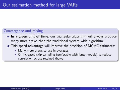
Convergence and mixing
In a given unit of time, our triangular algorithm will always producemany more draws than the traditional system-wide algorithm.
This speed advantage will improve the precision of MCMC estimates:
Many more draws to use in averagesOr increased skip-sampling (preferable with large models) to reducecorrelation across retained draws
Todd Clark (FRBC) Large VARs June 2016 23 / 41
Application 1: large structural VAR with SV
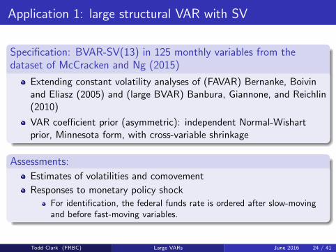
Specification: BVAR-SV(13) in 125 monthly variables from thedataset of McCracken and Ng (2015)
Extending constant volatility analyses of (FAVAR) Bernanke, Boivinand Eliasz (2005) and (large BVAR) Banbura, Giannone, and Reichlin(2010)
VAR coefficient prior (asymmetric): independent Normal-Wishartprior, Minnesota form, with cross-variable shrinkage
Assessments:
Estimates of volatilities and comovement
Responses to monetary policy shock
For identification, the federal funds rate is ordered after slow-movingand before fast-moving variables.
Todd Clark (FRBC) Large VARs June 2016 24 / 41

Application 1: large structural VAR with SV
Computation:
Model includes 203,250 VAR coefficients
On a 3.5 GHz Intel Core i7 processor, our algorithm produces 5000draws (after discarding 500 burning in) in just above 7 hours
The traditional system-based algorithm would be extremely difficult,just for memory requirements: the covariance matrix of the 203,250coefficients would require about 330 GB of RAM
Todd Clark (FRBC) Large VARs June 2016 25 / 41
Application 1: large structural VAR with SV
19701980199020002010
0.010.020.03
RPI
19701980199020002010
0.010.020.030.04
W875RX1
19701980199020002010
10 -3
2468101214DPCERA3M086SBEA
19701980199020002010
0.01
0.02
0.03CMRMTSPLx
19701980199020002010
0.01
0.02
0.03RETAILx
197019801990200020100.0050.010.0150.020.025
INDPRO
197019801990200020100.0050.010.0150.020.025
IPFPNSS
19701980199020002010
0.01
0.02
0.03IPFINAL
19701980199020002010
0.01
0.02
0.03IPCONGD
19701980199020002010
0.02
0.04
0.06
IPDCONGD
197019801990200020100.0050.010.0150.020.025
IPNCONGD
19701980199020002010
0.010.020.030.04
IPBUSEQ
19701980199020002010
0.01
0.02
0.03IPMAT
197019801990200020100.010.020.030.040.05
IPDMAT
19701980199020002010
0.010.020.030.04
IPNMAT
197019801990200020100.0050.010.0150.020.025
IPMANSICS
197019801990200020100.02
0.04
0.06
IPB51222S
19701980199020002010
0.02
0.04
0.06IPFUELS
19701980199020002010
0.51
1.52
CUMFNS
19701980199020002010
2
4
6HWI
19701980199020002010
10 -3
1
1.5
2HWIURATIO
19701980199020002010
10 -3
4
6
8CLF16OV
19701980199020002010
10 -3
2
4
6
8CE16OV
197019801990200020100.2
0.3
0.4
UNRATE
19701980199020002010
0.5
1
1.5UEMPMEAN
19701980199020002010
0.060.080.10.12
UEMPLT5
197019801990200020100.040.06
0.080.1
UEMP5TO14
197019801990200020100.04
0.06
0.08
0.1UEMP15OV
19701980199020002010
0.060.080.10.12
UEMP15T26
19701980199020002010
0.060.080.1
UEMP27OV
197019801990200020100.1
0.2
0.3CLAIMSx
19701980199020002010
10 -3
2
3
4PAYEMS
19701980199020002010
10 -3
4
6
8USGOOD
19701980199020002010
0.020.040.060.080.1
CES1021000001
197019801990200020100.005
0.01
0.015
0.02USCONS
19701980199020002010
10 -3
4
6
8MANEMP
19701980199020002010
10 -3
4681012
DMANEMP
19701980199020002010
10 -3
2
3
4
5NDMANEMP
19701980199020002010
10 -3
1.52
2.53
3.5
SRVPRD
19701980199020002010
10 -3
2345
USTPU
19701980199020002010
10 -3
2345
USWTRADE
19701980199020002010
10 -3
3456
USTRADE
19701980199020002010
10 -3
1.5
2
2.5
USFIRE
19701980199020002010
10 -3
3456
USGOVT
197019801990200020100.20.40.60.81
CES0600000007
19701980199020002010
0.1
0.2
0.3
AWOTMAN
19701980199020002010
0.20.40.60.8
AWHMAN
19701980199020002010
0.0050.010.015
BUSINVx
197019801990200020100.010.020.030.040.05
ISRATIOx
19701980199020002010
10 -3
2468
CES0600000008
197019801990200020100.0050.010.0150.020.025
CES2000000008
19701980199020002010
10 -3
468
CES3000000008
19701980199020002010
0.01
0.02
0.03PPIFGS
19701980199020002010
0.010.020.03
PPIFCG
197019801990200020100.0050.010.0150.020.025
PPIITM
197019801990200020100.020.040.060.080.1
PPICRM
19701980199020002010
0.1
0.2
0.3OILPRICEx
197019801990200020100.020.040.060.080.1
PPICMM
19701980199020002010
10 -3
2
4
6
8CPIAUCSL
19701980199020002010
10 -3
4681012
CPIAPPSL
197019801990200020100.010.020.030.04
CPITRNSL
19701980199020002010
10 -3
2
4
6CPIMEDSL
19701980199020002010
0.005
0.01
0.015
CUSR0000SAC
19701980199020002010
10 -3
2
4
6
8CUUR0000SAD
19701980199020002010
10 -3
2
4
6CUSR0000SAS
19701980199020002010
10 -3
2468
CPIULFSL
19701980199020002010
10 -3
4681012
CUUR0000SA0L2
19701980199020002010
10 -3
2
4
6
8CUSR0000SA0L5
19701980199020002010
10 -3
2
4
6PCEPI
19701980199020002010
10 -3
2
4
6
DDURRG3M086SBEA
197019801990200020100.005
0.01
0.015
0.02DNDGRG3M086SBEA
19701980199020002010
10 -3
2
3
4DSERRG3M086SBEA
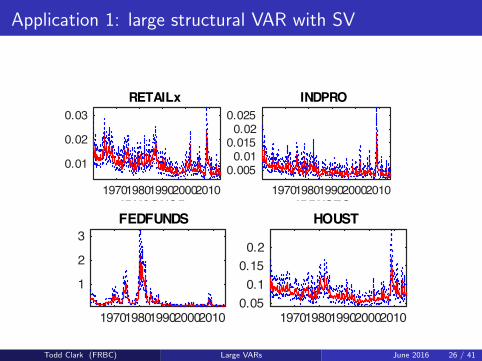
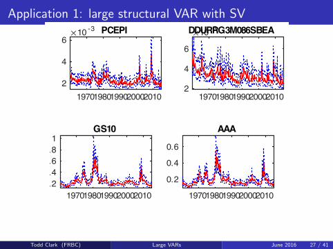
Figure 7: Posterior distribution of volatilities (diagonal elements of Σt ), slow variables.
19701980199020002010
1
2
3FEDFUNDS
197019801990200020100.050.10.150.2
HOUST
19701980199020002010
0.2
0.4
0.6
HOUSTNE
197019801990200020100.10.20.30.40.5
HOUSTMW
19701980199020002010
0.10.150.20.25
HOUSTS
197019801990200020100.1
0.2
0.3HOUSTW
197019801990200020100.020.040.060.08
AMDMNOx
19701980199020002010
0.01
0.015
0.02AMDMUOx
19701980199020002010
0.05
0.1
0.15S&P 500
19701980199020002010
0.05
0.1
0.15
S&P: indust
197019801990200020100.10.20.30.4
S&P div yield
19701980199020002010
0.05
0.1
0.15
S&P PE ratio
197019801990200020100.010.020.030.040.05
EXSZUSx
19701980199020002010
0.02
0.04
0.06
EXJPUSx
197019801990200020100.010.020.030.040.05
EXUSUKx
197019801990200020100.010.020.030.04
EXCAUSx
19701980199020002010
0.51
1.52
CP3Mx
19701980199020002010
0.51
1.52
TB3MS
19701980199020002010
0.51
1.5
TB6MS
19701980199020002010
0.51
1.52
GS1
197019801990200020100.20.40.60.81
1.2GS5
197019801990200020100.20.40.60.81
GS10
19701980199020002010
0.2
0.4
0.6
AAA
19701980199020002010
0.2
0.4
0.6BAA
19701980199020002010
0.51
1.5
COMPAPFFx
19701980199020002010
0.51
1.52
TB3SMFFM
19701980199020002010
0.51
1.52
TB6SMFFM
19701980199020002010
0.51
1.52
T1YFFM
197019801990200020100.51
1.52
2.5T5YFFM
197019801990200020100.51
1.52
2.5T10YFFM
19701980199020002010
1
2
3AAAFFM
19701980199020002010
1
2
3BAAFFM
197019801990200020100.010.020.030.040.05
M1SL
19701980199020002010
10 -3
2468101214
M2SL
19701980199020002010
10 -3
5
10
15M2REAL
19701980199020002010
0.05
0.1
0.15AMBSL
19701980199020002010
0.2
0.4
0.6TOTRESNS
19701980199020002010
2468
NONBORRES
197019801990200020100.0050.010.0150.020.025
BUSLOANS
197019801990200020100.0050.010.0150.020.025
REALLN
19701980199020002010
0.01
0.02
0.03
NONREVSL
19701980199020002010
10 -3
2345
CONSPI
19701980199020002010
0.005
0.01
0.015
MZMSL
197019801990200020100.020.040.060.080.10.12
DTCOLNVHFNM
197019801990200020100.020.040.060.080.1
DTCTHFNM
197019801990200020100.010.020.030.04
INVEST
19701980199020002010
4
6
8NAPMPI
197019801990200020102
4
6
NAPMEI
197019801990200020102345
NAPM
19701980199020002010
46810
NAPMNOI
197019801990200020102
4
6
NAPMSDI
19701980199020002010
4
6
8NAPMII
19701980199020002010
5
10
15NAPMPRI
Figure 8: Posterior distribution of volatilities (diagonal elements of Σt ), fast variables.
Todd Clark (FRBC) Large VARs June 2016 26 / 41
Application 1: large structural VAR with SV
19701980199020002010
0.010.020.03
RPI
19701980199020002010
0.010.020.030.04
W875RX1
19701980199020002010
10 -3
2468101214DPCERA3M086SBEA
19701980199020002010
0.01
0.02
0.03CMRMTSPLx
19701980199020002010
0.01
0.02
0.03RETAILx
197019801990200020100.0050.010.0150.020.025
INDPRO
197019801990200020100.0050.010.0150.020.025
IPFPNSS
19701980199020002010
0.01
0.02
0.03IPFINAL
19701980199020002010
0.01
0.02
0.03IPCONGD
19701980199020002010
0.02
0.04
0.06
IPDCONGD
197019801990200020100.0050.010.0150.020.025
IPNCONGD
19701980199020002010
0.010.020.030.04
IPBUSEQ
19701980199020002010
0.01
0.02
0.03IPMAT
197019801990200020100.010.020.030.040.05
IPDMAT
19701980199020002010
0.010.020.030.04
IPNMAT
197019801990200020100.0050.010.0150.020.025
IPMANSICS
197019801990200020100.02
0.04
0.06
IPB51222S
19701980199020002010
0.02
0.04
0.06IPFUELS
19701980199020002010
0.51
1.52
CUMFNS
19701980199020002010
2
4
6HWI
19701980199020002010
10 -3
1
1.5
2HWIURATIO
19701980199020002010
10 -3
4
6
8CLF16OV
19701980199020002010
10 -3
2
4
6
8CE16OV
197019801990200020100.2
0.3
0.4
UNRATE
19701980199020002010
0.5
1
1.5UEMPMEAN
19701980199020002010
0.060.080.10.12
UEMPLT5
197019801990200020100.040.06
0.080.1
UEMP5TO14
197019801990200020100.04
0.06
0.08
0.1UEMP15OV
19701980199020002010
0.060.080.10.12
UEMP15T26
19701980199020002010
0.060.080.1
UEMP27OV
197019801990200020100.1
0.2
0.3CLAIMSx
19701980199020002010
10 -3
2
3
4PAYEMS
19701980199020002010
10 -3
4
6
8USGOOD
19701980199020002010
0.020.040.060.080.1
CES1021000001
197019801990200020100.005
0.01
0.015
0.02USCONS
19701980199020002010
10 -3
4
6
8MANEMP
19701980199020002010
10 -3
4681012
DMANEMP
19701980199020002010
10 -3
2
3
4
5NDMANEMP
19701980199020002010
10 -3
1.52
2.53
3.5
SRVPRD
19701980199020002010
10 -3
2345
USTPU
19701980199020002010
10 -3
2345
USWTRADE
19701980199020002010
10 -3
3456
USTRADE
19701980199020002010
10 -3
1.5
2
2.5
USFIRE
19701980199020002010
10 -3
3456
USGOVT
197019801990200020100.20.40.60.81
CES0600000007
19701980199020002010
0.1
0.2
0.3
AWOTMAN
19701980199020002010
0.20.40.60.8
AWHMAN
19701980199020002010
0.0050.010.015
BUSINVx
197019801990200020100.010.020.030.040.05
ISRATIOx
19701980199020002010
10 -3
2468
CES0600000008
197019801990200020100.0050.010.0150.020.025
CES2000000008
19701980199020002010
10 -3
468
CES3000000008
19701980199020002010
0.01
0.02
0.03PPIFGS
19701980199020002010
0.010.020.03
PPIFCG
197019801990200020100.0050.010.0150.020.025
PPIITM
197019801990200020100.020.040.060.080.1
PPICRM
19701980199020002010
0.1
0.2
0.3OILPRICEx
197019801990200020100.020.040.060.080.1
PPICMM
19701980199020002010
10 -3
2
4
6
8CPIAUCSL
19701980199020002010
10 -3
4681012
CPIAPPSL
197019801990200020100.010.020.030.04
CPITRNSL
19701980199020002010
10 -3
2
4
6CPIMEDSL
19701980199020002010
0.005
0.01
0.015
CUSR0000SAC
19701980199020002010
10 -3
2
4
6
8CUUR0000SAD
19701980199020002010
10 -3
2
4
6CUSR0000SAS
19701980199020002010
10 -3
2468
CPIULFSL
19701980199020002010
10 -3
4681012
CUUR0000SA0L2
19701980199020002010
10 -3
2
4
6
8CUSR0000SA0L5
19701980199020002010
10 -3
2
4
6PCEPI
19701980199020002010
10 -3
2
4
6
DDURRG3M086SBEA
197019801990200020100.005
0.01
0.015
0.02DNDGRG3M086SBEA
19701980199020002010
10 -3
2
3
4DSERRG3M086SBEA
Figure 7: Posterior distribution of volatilities (diagonal elements of Σt ), slow variables.
19701980199020002010
1
2
3FEDFUNDS
197019801990200020100.050.10.150.2
HOUST
19701980199020002010
0.2
0.4
0.6
HOUSTNE
197019801990200020100.10.20.30.40.5
HOUSTMW
19701980199020002010
0.10.150.20.25
HOUSTS
197019801990200020100.1
0.2
0.3HOUSTW
197019801990200020100.020.040.060.08
AMDMNOx
19701980199020002010
0.01
0.015
0.02AMDMUOx
19701980199020002010
0.05
0.1
0.15S&P 500
19701980199020002010
0.05
0.1
0.15
S&P: indust
197019801990200020100.10.20.30.4
S&P div yield
19701980199020002010
0.05
0.1
0.15
S&P PE ratio
197019801990200020100.010.020.030.040.05
EXSZUSx
19701980199020002010
0.02
0.04
0.06
EXJPUSx
197019801990200020100.010.020.030.040.05
EXUSUKx
197019801990200020100.010.020.030.04
EXCAUSx
19701980199020002010
0.51
1.52
CP3Mx
19701980199020002010
0.51
1.52
TB3MS
19701980199020002010
0.51
1.5
TB6MS
19701980199020002010
0.51
1.52
GS1
197019801990200020100.20.40.60.81
1.2GS5
197019801990200020100.20.40.60.81
GS10
19701980199020002010
0.2
0.4
0.6
AAA
19701980199020002010
0.2
0.4
0.6BAA
19701980199020002010
0.51
1.5
COMPAPFFx
19701980199020002010
0.51
1.52
TB3SMFFM
19701980199020002010
0.51
1.52
TB6SMFFM
19701980199020002010
0.51
1.52
T1YFFM
197019801990200020100.51
1.52
2.5T5YFFM
197019801990200020100.51
1.52
2.5T10YFFM
19701980199020002010
1
2
3AAAFFM
19701980199020002010
1
2
3BAAFFM
197019801990200020100.010.020.030.040.05
M1SL
19701980199020002010
10 -3
2468101214
M2SL
19701980199020002010
10 -3
5
10
15M2REAL
19701980199020002010
0.05
0.1
0.15AMBSL
19701980199020002010
0.2
0.4
0.6TOTRESNS
19701980199020002010
2468
NONBORRES
197019801990200020100.0050.010.0150.020.025
BUSLOANS
197019801990200020100.0050.010.0150.020.025
REALLN
19701980199020002010
0.01
0.02
0.03
NONREVSL
19701980199020002010
10 -3
2345
CONSPI
19701980199020002010
0.005
0.01
0.015
MZMSL
197019801990200020100.020.040.060.080.10.12
DTCOLNVHFNM
197019801990200020100.020.040.060.080.1
DTCTHFNM
197019801990200020100.010.020.030.04
INVEST
19701980199020002010
4
6
8NAPMPI
197019801990200020102
4
6
NAPMEI
197019801990200020102345
NAPM
19701980199020002010
46810
NAPMNOI
197019801990200020102
4
6
NAPMSDI
19701980199020002010
4
6
8NAPMII
19701980199020002010
5
10
15NAPMPRI
Figure 8: Posterior distribution of volatilities (diagonal elements of Σt ), fast variables.
Todd Clark (FRBC) Large VARs June 2016 27 / 41
Application 1: large structural VAR with SV
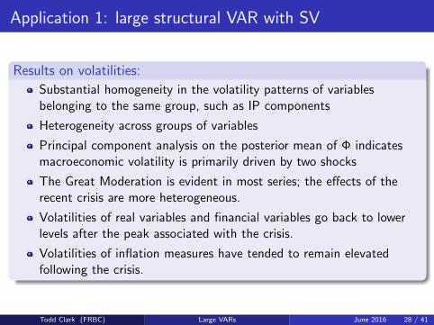
Results on volatilities:
Substantial homogeneity in the volatility patterns of variablesbelonging to the same group, such as IP components
Heterogeneity across groups of variables
Principal component analysis on the posterior mean of Φ indicatesmacroeconomic volatility is primarily driven by two shocks
The Great Moderation is evident in most series; the effects of therecent crisis are more heterogeneous.
Volatilities of real variables and financial variables go back to lowerlevels after the peak associated with the crisis.
Volatilities of inflation measures have tended to remain elevatedfollowing the crisis.
Todd Clark (FRBC) Large VARs June 2016 28 / 41
Application 1: large structural VAR with SV
12 24 36 48 60
10 -3
-10
-5
0RPI
12 24 36 48 60
10 -3
-10
-5
0W875RX1
12 24 36 48 60
10 -3
-10
-5
0DPCERA3M086SBEA
12 24 36 48 60
-0.02
-0.01
0CMRMTSPLx
12 24 36 48 60
10 -3
-5
0
5RETAILx
12 24 36 48 60-0.02
-0.01
0INDPRO
12 24 36 48 60
10 -3
-15-10-50
IPFPNSS
12 24 36 48 60
10 -3
-20
-10
0IPFINAL
12 24 36 48 60
10 -3
-10
-5
0IPCONGD
12 24 36 48 60-0.03
-0.02
-0.01
0IPDCONGD
12 24 36 48 60
10 -3
-8-6-4-20
IPNCONGD
12 24 36 48 60
-0.03-0.02-0.01
0IPBUSEQ
12 24 36 48 60
-0.02
-0.01
0IPMAT
12 24 36 48 60-0.03
-0.02
-0.01
0IPDMAT
12 24 36 48 60-0.02
-0.01
0IPNMAT
12 24 36 48 60-0.02
-0.01
0IPMANSICS
12 24 36 48 60
-0.02
-0.01
0
IPB51222S
12 24 36 48 60
10 -3
-10-505
IPFUELS
12 24 36 48 60
-1.5-1
-0.50
CUMFNS
12 24 36 48 60
-6-4-20
HWI
12 24 36 48 60
10 -3
-2
-1
0HWIURATIO
12 24 36 48 60
10 -3
-3-2-10
CLF16OV
12 24 36 48 60
10 -3
-8-6-4-20
CE16OV
12 24 36 48 600
0.2
0.4
0.6UNRATE
12 24 36 48 600
0.5
1
UEMPMEAN
12 24 36 48 600
0.02
0.04UEMPLT5
12 24 36 48 600
0.020.040.060.08
UEMP5TO14
12 24 36 48 600
0.050.10.15
UEMP15OV
12 24 36 48 600
0.05
0.1
UEMP15T26
12 24 36 48 600
0.1
0.2UEMP27OV
12 24 36 48 60
00.050.10.15
CLAIMSx
12 24 36 48 60
10 -3
-10
-5
0PAYEMS
12 24 36 48 60
-0.02
-0.01
0USGOOD
12 24 36 48 60
-0.02-0.01
00.01
CES1021000001
12 24 36 48 60-0.04
-0.02
0USCONS
12 24 36 48 60
10 -3
-15-10-50
MANEMP
12 24 36 48 60
-0.02
-0.01
0DMANEMP
12 24 36 48 60
10 -3
-8-6-4-20
NDMANEMP
12 24 36 48 60
10 -3
-8-6-4-20
SRVPRD
12 24 36 48 60
10 -3
-10
-5
0USTPU
12 24 36 48 60
10 -3
-10
-5
0USWTRADE
12 24 36 48 60
10 -3
-8-6-4-20
USTRADE
12 24 36 48 60
10 -3
-6-4-20
USFIRE
12 24 36 48 60
10 -3
-10
-5
0USGOVT
12 24 36 48 60
-0.1
-0.05
0CES0600000007
12 24 36 48 60
-0.1-0.05
0
AWOTMAN
12 24 36 48 60-0.15-0.1
-0.050
AWHMAN
12 24 36 48 60
10 -3
-10-50
BUSINVx
12 24 36 48 60
10 -3
-5051015
ISRATIOx
12 24 36 48 60
10 -3
-1
0
1CES0600000008
12 24 36 48 60
10 -3
-2
0
2CES2000000008
12 24 36 48 60
10 -3
-1
0
1CES3000000008
12 24 36 48 60
10 -3
-3-2-101
PPIFGS
12 24 36 48 60
10 -3
-2
0
2PPIFCG
12 24 36 48 60
10 -3
-2
0
2
PPIITM
12 24 36 48 60-0.01
0
0.01PPICRM
12 24 36 48 60
-0.02
0
0.02OILPRICEx
12 24 36 48 60
10 -3
-5051015
PPICMM
12 24 36 48 60
10 -3
-1
0
1CPIAUCSL
12 24 36 48 60
10 -3
-2-101
CPIAPPSL
12 24 36 48 60
10 -3
-20246
CPITRNSL
12 24 36 48 60
10 -4
-10-505
CPIMEDSL
12 24 36 48 60
10 -3
-1012
CUSR0000SAC
12 24 36 48 60
10 -3
-1012
CUUR0000SAD
12 24 36 48 60
10 -4
-15-10-505
CUSR0000SAS
12 24 36 48 60
10 -3
-1
0
1CPIULFSL
12 24 36 48 60
10 -3
-101
CUUR0000SA0L2
12 24 36 48 60
10 -3
-1
0
1CUSR0000SA0L5
12 24 36 48 60
10 -4
-10-505
PCEPI
12 24 36 48 60
10 -3
-1
0
1DDURRG3M086SBEA
12 24 36 48 60
10 -3
-2
0
2DNDGRG3M086SBEA
12 24 36 48 60
10 -4
-10-505
DSERRG3M086SBEA
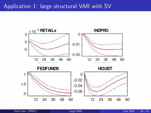
Figure 9: Impulse responses to a monetary policy shock: slow variables.
12 24 36 48 600
0.5
1FEDFUNDS
12 24 36 48 60
-0.06-0.04-0.02
0HOUST
12 24 36 48 60
-0.06-0.04-0.02
0HOUSTNE
12 24 36 48 60-0.08-0.06-0.04-0.02
00.02
HOUSTMW
12 24 36 48 60-0.06-0.04-0.02
0HOUSTS
12 24 36 48 60-0.08-0.06-0.04-0.02
00.02
HOUSTW
12 24 36 48 60-0.03-0.02-0.01
0
AMDMNOx
12 24 36 48 60-0.06
-0.04
-0.02
0AMDMUOx
12 24 36 48 60-0.03-0.02-0.01
00.01
S&P 500
12 24 36 48 60
-0.02
0
0.02S&P: indust
12 24 36 48 60-0.1
0
0.1S&P div yield
12 24 36 48 60
-0.020
0.020.040.06
S&P PE ratio
12 24 36 48 60
00.010.020.03
EXSZUSx
12 24 36 48 60-0.01
00.010.020.03
EXJPUSx
12 24 36 48 60
-0.04-0.03-0.02-0.01
EXUSUKx
12 24 36 48 60
10 -3
-50510
EXCAUSx
12 24 36 48 60
00.20.40.60.8
CP3Mx
12 24 36 48 60
00.20.40.6
TB3MS
12 24 36 48 60
00.20.40.6
TB6MS
12 24 36 48 60
00.20.40.6
GS1
12 24 36 48 600
0.2
0.4
GS5
12 24 36 48 60
0.10.20.30.4
GS10
12 24 36 48 600.10.20.30.4
AAA
12 24 36 48 600.10.20.30.40.5
BAA
12 24 36 48 60-0.4
-0.2
0COMPAPFFx
12 24 36 48 60
-0.4
-0.2
0TB3SMFFM
12 24 36 48 60
-0.4
-0.2
0TB6SMFFM
12 24 36 48 60
-0.4
-0.2
0T1YFFM
12 24 36 48 60-0.8-0.6-0.4-0.20
T5YFFM
12 24 36 48 60-0.8-0.6-0.4-0.20
0.2T10YFFM
12 24 36 48 60
-0.8-0.6-0.4-0.20
0.2AAAFFM
12 24 36 48 60-0.8-0.6-0.4-0.20
0.2BAAFFM
12 24 36 48 60
10 -3
-4
-2
0
2M1SL
12 24 36 48 60
10 -3
-1
0
1M2SL
12 24 36 48 60-0.02
-0.01
0M2REAL
12 24 36 48 60
10 -3
-4-2024
AMBSL
12 24 36 48 60-0.01
00.010.02
TOTRESNS
12 24 36 48 60
-0.1
0
0.1
NONBORRES
12 24 36 48 60
10 -3
-4
-2
0
BUSLOANS
12 24 36 48 60
10 -3
-3-2-101
REALLN
12 24 36 48 60
10 -3
-2
0
2NONREVSL
12 24 36 48 60
10 -3
-4
-2
0CONSPI
12 24 36 48 60
10 -3
-4
-2
0
MZMSL
12 24 36 48 60
10 -3
-10-505
DTCOLNVHFNM
12 24 36 48 60
10 -3
-6-4-2024
DTCTHFNM
12 24 36 48 60
10 -3
-20246
INVEST
12 24 36 48 60-2
-1
0NAPMPI
12 24 36 48 60-1.5-1
-0.50
NAPMEI
12 24 36 48 60-1.5-1
-0.50
NAPM
12 24 36 48 60-2
-1
0NAPMNOI
12 24 36 48 60-1.5-1
-0.50
0.5NAPMSDI
12 24 36 48 60
-1-0.50
0.5NAPMII
12 24 36 48 60-1.5-1
-0.50
0.5NAPMPRI
Figure 10: Impulse responses to a monetary policy shock: fast variables.
Todd Clark (FRBC) Large VARs June 2016 29 / 41
Application 1: large structural VAR with SV
12 24 36 48 60
10 -3
-10
-5
0RPI
12 24 36 48 60
10 -3
-10
-5
0W875RX1
12 24 36 48 60
10 -3
-10
-5
0DPCERA3M086SBEA
12 24 36 48 60
-0.02
-0.01
0CMRMTSPLx
12 24 36 48 60
10 -3
-5
0
5RETAILx
12 24 36 48 60-0.02
-0.01
0INDPRO
12 24 36 48 60
10 -3
-15-10-50
IPFPNSS
12 24 36 48 60
10 -3
-20
-10
0IPFINAL
12 24 36 48 60
10 -3
-10
-5
0IPCONGD
12 24 36 48 60-0.03
-0.02
-0.01
0IPDCONGD
12 24 36 48 60
10 -3
-8-6-4-20
IPNCONGD
12 24 36 48 60
-0.03-0.02-0.01
0IPBUSEQ
12 24 36 48 60
-0.02
-0.01
0IPMAT
12 24 36 48 60-0.03
-0.02
-0.01
0IPDMAT
12 24 36 48 60-0.02
-0.01
0IPNMAT
12 24 36 48 60-0.02
-0.01
0IPMANSICS
12 24 36 48 60
-0.02
-0.01
0
IPB51222S
12 24 36 48 60
10 -3
-10-505
IPFUELS
12 24 36 48 60
-1.5-1
-0.50
CUMFNS
12 24 36 48 60
-6-4-20
HWI
12 24 36 48 60
10 -3
-2
-1
0HWIURATIO
12 24 36 48 60
10 -3
-3-2-10
CLF16OV
12 24 36 48 60
10 -3
-8-6-4-20
CE16OV
12 24 36 48 600
0.2
0.4
0.6UNRATE
12 24 36 48 600
0.5
1
UEMPMEAN
12 24 36 48 600
0.02
0.04UEMPLT5
12 24 36 48 600
0.020.040.060.08
UEMP5TO14
12 24 36 48 600
0.050.10.15
UEMP15OV
12 24 36 48 600
0.05
0.1
UEMP15T26
12 24 36 48 600
0.1
0.2UEMP27OV
12 24 36 48 60
00.050.10.15
CLAIMSx
12 24 36 48 60
10 -3
-10
-5
0PAYEMS
12 24 36 48 60
-0.02
-0.01
0USGOOD
12 24 36 48 60
-0.02-0.01
00.01
CES1021000001
12 24 36 48 60-0.04
-0.02
0USCONS
12 24 36 48 60
10 -3
-15-10-50
MANEMP
12 24 36 48 60
-0.02
-0.01
0DMANEMP
12 24 36 48 60
10 -3
-8-6-4-20
NDMANEMP
12 24 36 48 60
10 -3
-8-6-4-20
SRVPRD
12 24 36 48 60
10 -3
-10
-5
0USTPU
12 24 36 48 60
10 -3
-10
-5
0USWTRADE
12 24 36 48 60
10 -3
-8-6-4-20
USTRADE
12 24 36 48 60
10 -3
-6-4-20
USFIRE
12 24 36 48 60
10 -3
-10
-5
0USGOVT
12 24 36 48 60
-0.1
-0.05
0CES0600000007
12 24 36 48 60
-0.1-0.05
0
AWOTMAN
12 24 36 48 60-0.15-0.1
-0.050
AWHMAN
12 24 36 48 60
10 -3
-10-50
BUSINVx
12 24 36 48 60
10 -3
-5051015
ISRATIOx
12 24 36 48 60
10 -3
-1
0
1CES0600000008
12 24 36 48 60
10 -3
-2
0
2CES2000000008
12 24 36 48 60
10 -3
-1
0
1CES3000000008
12 24 36 48 60
10 -3
-3-2-101
PPIFGS
12 24 36 48 60
10 -3
-2
0
2PPIFCG
12 24 36 48 60
10 -3
-2
0
2
PPIITM
12 24 36 48 60-0.01
0
0.01PPICRM
12 24 36 48 60
-0.02
0
0.02OILPRICEx
12 24 36 48 60
10 -3
-5051015
PPICMM
12 24 36 48 60
10 -3
-1
0
1CPIAUCSL
12 24 36 48 60
10 -3
-2-101
CPIAPPSL
12 24 36 48 60
10 -3
-20246
CPITRNSL
12 24 36 48 60
10 -4
-10-505
CPIMEDSL
12 24 36 48 60
10 -3
-1012
CUSR0000SAC
12 24 36 48 60
10 -3
-1012
CUUR0000SAD
12 24 36 48 60
10 -4
-15-10-505
CUSR0000SAS
12 24 36 48 60
10 -3
-1
0
1CPIULFSL
12 24 36 48 60
10 -3
-101
CUUR0000SA0L2
12 24 36 48 60
10 -3
-1
0
1CUSR0000SA0L5
12 24 36 48 60
10 -4
-10-505
PCEPI
12 24 36 48 60
10 -3
-1
0
1DDURRG3M086SBEA
12 24 36 48 60
10 -3
-2
0
2DNDGRG3M086SBEA
12 24 36 48 60
10 -4
-10-505
DSERRG3M086SBEA
Figure 9: Impulse responses to a monetary policy shock: slow variables.
12 24 36 48 600
0.5
1FEDFUNDS
12 24 36 48 60
-0.06-0.04-0.02
0HOUST
12 24 36 48 60
-0.06-0.04-0.02
0HOUSTNE
12 24 36 48 60-0.08-0.06-0.04-0.02
00.02
HOUSTMW
12 24 36 48 60-0.06-0.04-0.02
0HOUSTS
12 24 36 48 60-0.08-0.06-0.04-0.02
00.02
HOUSTW
12 24 36 48 60-0.03-0.02-0.01
0
AMDMNOx
12 24 36 48 60-0.06
-0.04
-0.02
0AMDMUOx
12 24 36 48 60-0.03-0.02-0.01
00.01
S&P 500
12 24 36 48 60
-0.02
0
0.02S&P: indust
12 24 36 48 60-0.1
0
0.1S&P div yield
12 24 36 48 60
-0.020
0.020.040.06
S&P PE ratio
12 24 36 48 60
00.010.020.03
EXSZUSx
12 24 36 48 60-0.01
00.010.020.03
EXJPUSx
12 24 36 48 60
-0.04-0.03-0.02-0.01
EXUSUKx
12 24 36 48 60
10 -3
-50510
EXCAUSx
12 24 36 48 60
00.20.40.60.8
CP3Mx
12 24 36 48 60
00.20.40.6
TB3MS
12 24 36 48 60
00.20.40.6
TB6MS
12 24 36 48 60
00.20.40.6
GS1
12 24 36 48 600
0.2
0.4
GS5
12 24 36 48 60
0.10.20.30.4
GS10
12 24 36 48 600.10.20.30.4
AAA
12 24 36 48 600.10.20.30.40.5
BAA
12 24 36 48 60-0.4
-0.2
0COMPAPFFx
12 24 36 48 60
-0.4
-0.2
0TB3SMFFM
12 24 36 48 60
-0.4
-0.2
0TB6SMFFM
12 24 36 48 60
-0.4
-0.2
0T1YFFM
12 24 36 48 60-0.8-0.6-0.4-0.20
T5YFFM
12 24 36 48 60-0.8-0.6-0.4-0.20
0.2T10YFFM
12 24 36 48 60
-0.8-0.6-0.4-0.20
0.2AAAFFM
12 24 36 48 60-0.8-0.6-0.4-0.20
0.2BAAFFM
12 24 36 48 60
10 -3
-4
-2
0
2M1SL
12 24 36 48 60
10 -3
-1
0
1M2SL
12 24 36 48 60-0.02
-0.01
0M2REAL
12 24 36 48 60
10 -3
-4-2024
AMBSL
12 24 36 48 60-0.01
00.010.02
TOTRESNS
12 24 36 48 60
-0.1
0
0.1
NONBORRES
12 24 36 48 60
10 -3
-4
-2
0
BUSLOANS
12 24 36 48 60
10 -3
-3-2-101
REALLN
12 24 36 48 60
10 -3
-2
0
2NONREVSL
12 24 36 48 60
10 -3
-4
-2
0CONSPI
12 24 36 48 60
10 -3
-4
-2
0
MZMSL
12 24 36 48 60
10 -3
-10-505
DTCOLNVHFNM
12 24 36 48 60
10 -3
-6-4-2024
DTCTHFNM
12 24 36 48 60
10 -3
-20246
INVEST
12 24 36 48 60-2
-1
0NAPMPI
12 24 36 48 60-1.5-1
-0.50
NAPMEI
12 24 36 48 60-1.5-1
-0.50
NAPM
12 24 36 48 60-2
-1
0NAPMNOI
12 24 36 48 60-1.5-1
-0.50
0.5NAPMSDI
12 24 36 48 60
-1-0.50
0.5NAPMII
12 24 36 48 60-1.5-1
-0.50
0.5NAPMPRI
Figure 10: Impulse responses to a monetary policy shock: fast variables.
Todd Clark (FRBC) Large VARs June 2016 30 / 41
Application 1: large structural VAR with SV
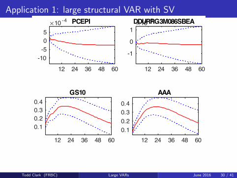
Results on impulse responses to FFR shock:
The patterns of impulse responses align with typical structuralmodels: significant deterioration in real activity, very limited pricepuzzle, a significant deterioration in stock prices, and a less thanproportional increase in the entire term structure
Inclusion of SV does not affect substantially the VAR coefficientestimates with respect to Banbura, Giannone and Reichlin (2010)
But it matters for inference and time variation in variancecontributions and shares
Todd Clark (FRBC) Large VARs June 2016 31 / 41
Application 2: forecasts of 20 monthly variables
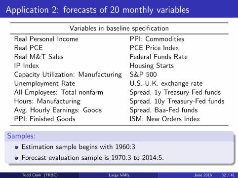
Variables in baseline specification
Real Personal Income PPI: CommoditiesReal PCE PCE Price IndexReal M&T Sales Federal Funds RateIP Index Housing StartsCapacity Utilization: Manufacturing S&P 500Unemployment Rate U.S.-U.K. exchange rateAll Employees: Total nonfarm Spread, 1y Treasury-Fed fundsHours: Manufacturing Spread, 10y Treasury-Fed fundsAvg. Hourly Earnings: Goods Spread, Baa-Fed fundsPPI: Finished Goods ISM: New Orders Index
Samples:
Estimation sample begins with 1960:3
Forecast evaluation sample is 1970:3 to 2014:5.
Todd Clark (FRBC) Large VARs June 2016 32 / 41
Application 2: forecasts of 20 monthly variables
Four models:
3-variable BVAR, homoskedastic: growth rate of IP (∆ ln IP), PCEinflation (∆ lnPECEPI ), fed funds rate (FFR)
3-variable BVAR-SV
20-variable BVAR, homoskedastic
20-variable BVAR-SV
Todd Clark (FRBC) Large VARs June 2016 33 / 41
Application 2: forecasts of 20 monthly variables
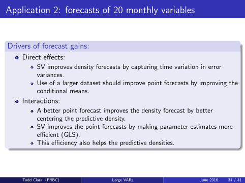
Drivers of forecast gains:
Direct effects:
SV improves density forecasts by capturing time variation in errorvariances.Use of a larger dataset should improve point forecasts by improving theconditional means.
Interactions:
A better point forecast improves the density forecast by bettercentering the predictive density.SV improves the point forecasts by making parameter estimates moreefficient (GLS).This efficiency also helps the predictive densities.
Todd Clark (FRBC) Large VARs June 2016 34 / 41
Application 2: forecasts of 20 monthly variables
step-ahead1 2 3 4 5 6 7 8 9 10 11 12
0.98
1
1.02
1.04
1.06
1.08
1.1
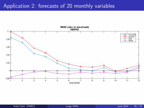
RMSE (ratio to benchmark)INDPRO
step-ahead1 2 3 4 5 6 7 8 9 10 11 12
0.96
0.97
0.98
0.99
1
1.01
1.02
1.03
1.04
1.05
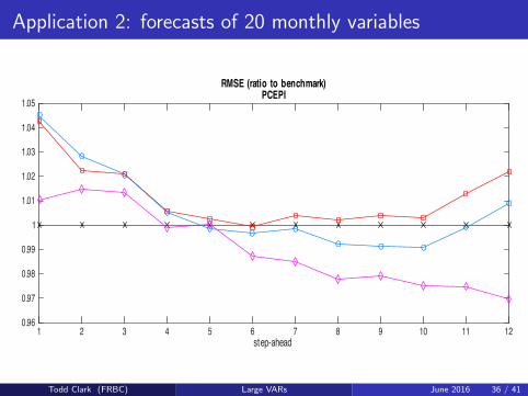
RMSE (ratio to benchmark)PCEPI
step-ahead1 2 3 4 5 6 7 8 9 10 11 12
0.92
0.94
0.96
0.98
1
1.02
1.04
1.06
1.08
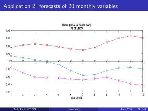
RMSE (ratio to benchmark)FEDFUNDS
homo20homo3SV3SV20
Figure 14: Point forecasts: relative RMSE of di§erent models. Black line (benchmark, marker:
crosses) is a homoschedastic VAR with 20 variables, red line (marker: squares) is a homoschedastic
VAR with 3 variables, blue line (marker: circles) is heteroschedastic VAR with 3 variables, purple
line (marker: diamonds) is heteroschedastic VAR with 20 variables.
Todd Clark (FRBC) Large VARs June 2016 35 / 41
Application 2: forecasts of 20 monthly variablesstep-ahead
1 2 3 4 5 6 7 8 9 10 11 120.98
1
1.02
1.04
1.06
1.08
1.1
RMSE (ratio to benchmark)INDPRO
step-ahead1 2 3 4 5 6 7 8 9 10 11 12
0.96
0.97
0.98
0.99
1
1.01
1.02
1.03
1.04
1.05
RMSE (ratio to benchmark)PCEPI
step-ahead1 2 3 4 5 6 7 8 9 10 11 12
0.92
0.94
0.96
0.98
1
1.02
1.04
1.06
1.08
RMSE (ratio to benchmark)FEDFUNDS
homo20homo3SV3SV20
Figure 14: Point forecasts: relative RMSE of di§erent models. Black line (benchmark, marker:
crosses) is a homoschedastic VAR with 20 variables, red line (marker: squares) is a homoschedastic
VAR with 3 variables, blue line (marker: circles) is heteroschedastic VAR with 3 variables, purple
line (marker: diamonds) is heteroschedastic VAR with 20 variables.
Todd Clark (FRBC) Large VARs June 2016 36 / 41
Application 2: forecasts of 20 monthly variables
step-ahead1 2 3 4 5 6 7 8 9 10 11 12
0.98
1
1.02
1.04
1.06
1.08
1.1
RMSE (ratio to benchmark)INDPRO
step-ahead1 2 3 4 5 6 7 8 9 10 11 12
0.96
0.97
0.98
0.99
1
1.01
1.02
1.03
1.04
1.05
RMSE (ratio to benchmark)PCEPI
step-ahead1 2 3 4 5 6 7 8 9 10 11 12
0.92
0.94
0.96
0.98
1
1.02
1.04
1.06
1.08
RMSE (ratio to benchmark)FEDFUNDS
homo20homo3SV3SV20
Figure 14: Point forecasts: relative RMSE of di§erent models. Black line (benchmark, marker:
crosses) is a homoschedastic VAR with 20 variables, red line (marker: squares) is a homoschedastic
VAR with 3 variables, blue line (marker: circles) is heteroschedastic VAR with 3 variables, purple
line (marker: diamonds) is heteroschedastic VAR with 20 variables.
Todd Clark (FRBC) Large VARs June 2016 37 / 41
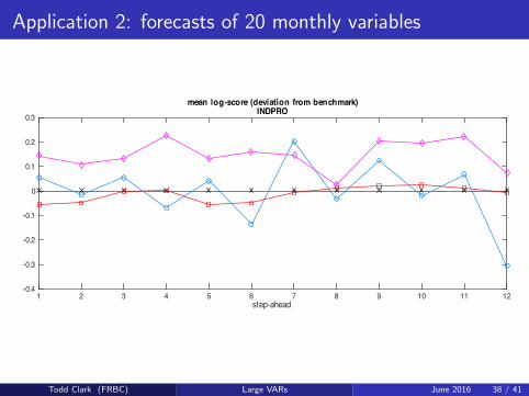
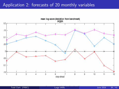
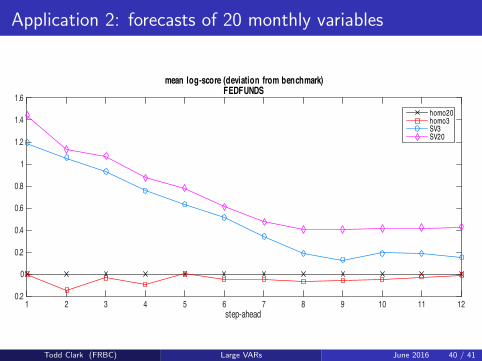
Application 2: forecasts of 20 monthly variables
step-ahead1 2 3 4 5 6 7 8 9 10 11 12
-0.4
-0.3
-0.2
-0.1
0
0.1
0.2
0.3
mean log-score (deviation from benchmark)INDPRO
step-ahead1 2 3 4 5 6 7 8 9 10 11 12
-0.15
-0.1
-0.05
0
0.05
0.1
0.15
0.2
mean log-score (deviation from benchmark)PCEPI
step-ahead1 2 3 4 5 6 7 8 9 10 11 12
-0.2
0
0.2
0.4
0.6
0.8
1
1.2
1.4
1.6
mean log-score (deviation from benchmark)FEDFUNDS
homo20homo3SV3SV20
Figure 15: Point forecasts: Log-score gains of di§erent models vs benchmark. Black line (bench-
mark, marker: crosses) is a homoschedastic VAR with 20 variables, red line (marker: squares) is a
homoschedastic VAR with 3 variables, blue line (marker: circles) is heteroschedastic VAR with 3
variables, purple line (marker: diamonds) is heteroschedastic VAR with 20 variables.
Todd Clark (FRBC) Large VARs June 2016 38 / 41
Application 2: forecasts of 20 monthly variablesstep-ahead
1 2 3 4 5 6 7 8 9 10 11 12-0.4
-0.3
-0.2
-0.1
0
0.1
0.2
0.3
mean log-score (deviation from benchmark)INDPRO
step-ahead1 2 3 4 5 6 7 8 9 10 11 12
-0.15
-0.1
-0.05
0
0.05
0.1
0.15
0.2
mean log-score (deviation from benchmark)PCEPI
step-ahead1 2 3 4 5 6 7 8 9 10 11 12
-0.2
0
0.2
0.4
0.6
0.8
1
1.2
1.4
1.6
mean log-score (deviation from benchmark)FEDFUNDS
homo20homo3SV3SV20
Figure 15: Point forecasts: Log-score gains of di§erent models vs benchmark. Black line (bench-
mark, marker: crosses) is a homoschedastic VAR with 20 variables, red line (marker: squares) is a
homoschedastic VAR with 3 variables, blue line (marker: circles) is heteroschedastic VAR with 3
variables, purple line (marker: diamonds) is heteroschedastic VAR with 20 variables.
Todd Clark (FRBC) Large VARs June 2016 39 / 41
Application 2: forecasts of 20 monthly variables
step-ahead1 2 3 4 5 6 7 8 9 10 11 12
-0.4
-0.3
-0.2
-0.1
0
0.1
0.2
0.3
mean log-score (deviation from benchmark)INDPRO
step-ahead1 2 3 4 5 6 7 8 9 10 11 12
-0.15
-0.1
-0.05
0
0.05
0.1
0.15
0.2
mean log-score (deviation from benchmark)PCEPI
step-ahead1 2 3 4 5 6 7 8 9 10 11 12
-0.2
0
0.2
0.4
0.6
0.8
1
1.2
1.4
1.6
mean log-score (deviation from benchmark)FEDFUNDS
homo20homo3SV3SV20
Figure 15: Point forecasts: Log-score gains of di§erent models vs benchmark. Black line (bench-
mark, marker: crosses) is a homoschedastic VAR with 20 variables, red line (marker: squares) is a
homoschedastic VAR with 3 variables, blue line (marker: circles) is heteroschedastic VAR with 3
variables, purple line (marker: diamonds) is heteroschedastic VAR with 20 variables.
Todd Clark (FRBC) Large VARs June 2016 40 / 41
Conclusions
We develop a new approach that makes feasible fully Bayesianinference of large BVARs with SV.
Also makes feasible the use of asymmetric priors (independent N-Wpriors) with SV or constant volatility, in large models
The method is based on a straightforward triangularization of thesystem, and it is very simple to implement by modifying existing codefor drawing VAR coefficients.
The algorithm ensures computational gains of order N2 and yieldsbetter mixing and convergence properties.
Todd Clark (FRBC) Large VARs June 2016 41 / 41