RESEARCH ARTICLE

Spatial resolution of PIV for the measurement of turbulence

P. Lavoie Æ G. Avallone Æ F. De Gregorio ÆG. P. Romano Æ R. A. Antonia

Received: 25 September 2006 / Revised: 20 April 2007 / Accepted: 20 April 2007 / Published online: 30 May 2007

� Springer-Verlag 2007

Abstract Recent technological advancements have made

the use of particle image velocimetry (PIV) more wide-

spread for studying turbulent flows over a wide range of

scales. Although PIV does not threaten to make obsolete

more mature techniques, such as hot-wire anemometry

(HWA), it is justifiably becoming an increasingly impor-

tant tool for turbulence research. This paper assesses the

ability of PIV to resolve all relevant scales in a classical

turbulent flow, namely grid turbulence, via a comparison

with theoretical predictions as well as HWA measure-

ments. Particular attention is given to the statistical con-

vergence of mean turbulent quantities and the spatial

resolution of PIV. An analytical method is developed to

quantify and correct for the effect of the finite spatial res-

olution of PIV measurements. While the present uncor-

rected PIV results largely underestimate the mean turbulent

kinetic energy and energy dissipation rate, the corrected

measurements agree to a close approximation with the

HWA data. The transport equation for the second-order

structure function in grid turbulence is used to establish the

range of scales affected by the limited resolution. The

results show that PIV, due to the geometry of its sensing

domain, must meet slightly more stringent requirements in

terms of resolution, compared with HWA, in order to

provide reliable measurements in turbulence.

1 Introduction

Non-intrusive laser-based techniques, such as laser Dopp-

ler velocimetry (LDV) and particle image velocimetry

(PIV), are being used more widely for turbulence mea-

surements. Although these techniques offer various

advantages over more traditional methods (e.g. hot-wire

anemometry—HWA), their ability to resolve adequately all

scales of interest for turbulence studies has yet to be

established rigorously, particularly in the case of PIV. It is

therefore important that these techniques are properly

validated, in order to assess their spatial resolution limi-

tations and investigate the impact of advancements related

to each technique. This type of approach has been suc-

cessfully implemented in the improvement of LDV data

reduction schemes, as they pertain to improved frequency

resolution (Muller et al. 1998; Van Maanen et al. 1999). In

the case of PIV, Westerweel et al. (1997) improved the

spatial resolution by nearly a factor of 10, through the use

of a window offset. Only very recently have there been

attempts to quantify the effect of the limited spatial reso-

lution associated with the finite size of the interrogation

window in PIV (Scarano 2003; Foucaut et al. 2004; Sai-

krishnan et al. 2006; Poelma et al. 2006). Although PIV

has demonstrated strong improvements in the description

of small scales, there is still an open question relative to the

P. Lavoie (&)

Department of Aeronautics, Imperial College London,

London, UK

e-mail: p.lavoie@imperial.ac.uk

G. Avallone � G. P. Romano

Department of Mechanics and Aeronautics,

University ‘‘La Sapienza’’, Rome, Italy

F. De Gregorio

CIRA, Italian Aerospace Center, Capua, Italy

R. A. Antonia

Discipline of Mechanical Engineering,

University of Newcastle, Callagan, NSW, Australia

123

Exp Fluids (2007) 43:39–51

DOI 10.1007/s00348-007-0319-x

effect of resolution on its ability to capture accurately the

inertial and dissipative ranges.

There are two main issues that emerge when imple-

menting validation procedures for a particular measure-

ment technique. Firstly, it is important to select a flow

for which theoretical results, especially in connection

with the flow properties of interest (in this case, the small

scales of turbulence), are known with a high level of

confidence. Secondly, it is desirable to compare the

technique against a method that has good temporal and

spatial resolutions. With regard to the first issue, homo-

geneous isotropic turbulence (HIT) is ideal from a theo-

retical viewpoint, while a close approximation of this flow

is provided by the decaying turbulence downstream of a

grid. Much has been learned from the previous works on

grid turbulence since the seminal papers by Batchelor and

Townsend (1947, 1948), and Comte-Bellot and Corrsin

(1966). However, some aspects of this flow remain un-

clear, such as the possible dependence of the turbulence

statistics on initial conditions (e.g. the shape and size of

the grid mesh, see for instance the thorough discussions

given by George et al. 2001). Notwithstanding these pos-

sible effects, the turbulent kinetic energy dissipation rate

(simply dissipation hereafter) can be estimated indirectly

with high accuracy from the kinetic energy budget

(Corrsin 1963),

eh id ¼ �U

2

d q2� �

dx1

; ð1Þ

where U is the mean flow velocity, hq2i � hu21i

�

þhu22i þ hu2

3iÞ is twice the turbulent kinetic energy, hidenotes time averaging and the subscript d indicates that

hei is determined from the kinetic energy decay, i.e. (1).

For grid turbulence, Taylor’s hypothesis is used to

transform the time t into a streamwise distance x1, viz.

¶x1 = –U¶t. Equation (1) is of considerable importance

since hei is a quantity that is notoriously difficult to

determine in experiments. An additional advantage of HIT

is that the transport equation for the two-point velocity

correlation function is known exactly for this flow (Karman

and Howarth 1938). The Karman–Howarth equation can be

re-expressed in terms of the velocity structure functions

(Saffman 1968; Danaila et al. 1999), viz.

� diuið Þ3D E

¼ 4

5eh iri � 6m

d

dridiuið Þ2

D Eþ Iui

ð2Þ

where hðdjuiÞni � h½uiðxþ rjÞ � uiðxÞ�ni; m is the kinetic

viscosity, rj is a separation vector taken along the xj-axis,

and no summation is implied over indices. In grid

turbulence, the streamwise decay is represented by the

non-stationary term Iui; which is expressed as

Iui� � 3U

r4i

Z ri

0

s4 o

ox1

diuið Þ2D E

ds; ð3Þ

where s is a dummy variable. Expression (2) can be

interpreted as a scale-by-scale turbulent energy budget and,

as shown below, can be used to quantify the effects of the

limited resolution on the different scales of the turbulence.

Concerning the second issue, HWA offers good temporal

and spatial resolution, and has been tested extensively in grid

turbulence. With suitably chosen experimental conditions,

accurate estimates of hei as well as the mean enstrophy have

been obtained with this method (e.g. Foss and Wallace 1989;

Sirivat and Warhaft 1983; Mydlarski and Warhaft 1996;

Antonia et al. 1998; Zhou and Antonia 2000b; Zhou et al.

2003; Gagne et al. 2004; Lavoie et al. 2007). It should also

be noted that the availability of direct numerical simulations

(not only for HIT but also in wall shear flows) has contrib-

uted to the development and validations of techniques to

correct hot-wire measurements for the effect of finite spatial

resolution of the probe (e.g. Suzuki and Kasagi 1992;

Antonia 1993; Kim and Antonia 1993; Ewing et al. 1995;

Zhu and Antonia 1995; Moin and Mahesh 1998; Antonia

et al. 2002). A comparison with HWA can thus be beneficial

to assess the ability of PIV (or any other non-intrusive

method) to resolve the small-scale motion adequately.

In this paper, PIV and HWA measurements in decaying

turbulence behind a woven mesh grid are reported. The first

objective is to establish the range of scales over which PIV

measurements can be considered reliable (at least for this

type of flow) by comparing the two sets of measurements for

similar initial conditions. Analytical equations are derived to

account for the finite spatial resolution of the PIV, similarly

to what has been proposed for HWA (e.g. Wyngaard 1968;

Zhu and Antonia 1995, 1996). The effect of resolution on the

turbulent kinetic energy, dissipation rate, velocity structure

functions and scale-by-scale energy budget are considered.

The focus here is on the intermediate-far range

(30 � x1=M � 60; with M the mesh size) where turbulence

intensities are low (less than 3%). For the present purpose,

the experimental conditions and spatial resolution of each

measurement technique have been chosen so that HWA

provides adequately resolved measurements, while the res-

olution of the PIV is purposefully stretched to test its limits

in a meaningful manner. This also provides a relatively

stringent benchmark against which the effectiveness of the

correction method presented in Sect. 2 can be assessed.

2 Experimental details

The PIV tests were performed in the CIRA low speed wind

tunnel (CT-1), which is an Eiffel type open circuit wind

40 Exp Fluids (2007) 43:39–51

123

tunnel, with the following properties: velocity range from

5–55 m/s, nozzle contraction ratio of 16:1 and a maximum

turbulence level of 0.2% at 10 m/s and 0.1% at 50 m/s. The

working section was 600 mm long, 302 mm wide and

302 mm high with full optical access. A grid made of

woven wires (diameter d = 1.2 mm) with mesh size

M = 4.5 mm was mounted immediately downstream of the

contraction, i.e. at the beginning of the working section.

The solidity of the grid, r � d=Mð2� d=MÞ; was 0.45 and

a Reynolds number, RM = UM/m, of 3000 was used (i.e.

mean flow velocity U = 10 m/s). The pressure gradient in

the working section was nearly zero (roughly 1% of the

dynamic pressure in the tunnel for U = 10 m/s).

A Nd–Yag laser (pulse energy of 300 mJ at a wave-

length of 532 nm) was used and images of tracer particles

(Di-Sebacate oil with an average diameter of 2 lm) were

acquired by a PCO SensiCam at a resolution of

1,280 · 1,024 pixels (12 bit grey level resolution) syn-

chronised with the laser emission (the objective focal

length was 100 mm, while the f-number was 5.6). Typical

images correspond to a region of 80 mm along x1 and

65 mm along x2, or about 18M · 14M (the magnification

factor was about 15 pixel/mm), while the depth of view

was roughly 1 mm due to the laser sheet thickness. This

image size was equivalent to roughly five integral length

scales and therefore allowed the large scales of the flow to

be captured. On an average, the tracer particle size on the

images was about three pixels. A time delay (Dt) of around

90 ls, which yielded particle displacements of around 16

pixels at x/M = 50, was selected to be optimum based on

preliminary investigations. At this location, the turbulence

intensity (TI) was about 2%, equivalent to a displacement

of roughly 0.3 pixels. This provided a dynamic range of

about 50; sufficient for capturing the streamwise decay of

the turbulence (Poelma et al. 2006). The turbulence

intensity further downstream was too low for the PIV to

capture the velocity fluctuations (e.g. at x/M = 100, TI

dropped to 1% and the velocity fluctuations were under

0.1 pixels; dynamic range equal to 80). Therefore, the PIV

measurements presented here are limited to x/M £ 50.

Measurements of the decaying turbulence over a distance

greater than 18 M were obtained by overlapping acquisition

regions along the streamwise direction. Images were pro-

cessed with the PivView code using standard multi-pass

cross-correlations between consecutive images. Interroga-

tion windows (size 32 · 32 pixels, or approximately 2

· 2 mm2, yielded about 20–25 particles per window) were

overlapped over half their width (16 pixels). The selection

of this interrogation window size was a result of a com-

promise between spatial resolution and data quality

requirements. Smaller windows significantly increase the

number of spurious velocity vectors due to a reduction in

the number of particles for each window. Although ad-

vanced image deformation algorithms can increase the

spatial resolution of PIV (as reported in the results of PIV

Challenges 2001, 2003, 2005; see http://www.pivchal-

lenge.org), the present PIV data were obtained without

deformation of the interrogation window or of the whole

image. This was done for two reasons. First, it gives some

general insights for the investigation of a wide range of

flow scales with PIV without the use of more advanced

algorithms. Second, the sensitivity of PIV to changes in

velocity can be simply approximated to be uniformed over

the measurement region. This allows the results of the

spectral correction analysis (given below) to be more

generally applicable. Turbulence statistics were computed

over approximately 1,000 images. Homogeneity along the

x2-axis, which was satisfied to within ±1.5% for the mean

flow, allowed further averaging of turbulence statistics

along the vertical axis. Velocity fluctuations were consid-

ered relative to the local mean velocity before averaging to

avoid errors due to a possible inhomogeneity of the mean

flow.

The HWA measurements were performed in an open

circuit wind tunnel at the University of Newcastle. The grid

was located immediately downstream of a 9:1 contraction.

The working section of the tunnel was 2.4 m long and its

square cross-section at the contraction had a width

350 mm. The floor was inclined slightly to provide a zero

pressure gradient (the pressure change was less than 0.4%

of dynamic pressure in tunnel). The grid used was of the

same geometry and wire diameter as for the PIV experi-

ments (woven mesh with d = 1.2 mm). However, the mesh

size was slightly larger, M = 5.1 mm compared to 4.5 mm,

which resulted in a grid solidity of r = 0.42. Due to the

slight difference in mesh length, the mean flow velocity

was selected to give the same RM as for the PIV (i.e.

U = 9.1 m/s). Lavoie et al. (2007) found that r only has a

very weak effect on the decay and structure of the turbu-

lence. Therefore, the slight difference between the solidi-

ties of the woven meshes used in the PIV and HWA

experiments does not represent a significant change in

initial conditions. The background turbulence intensity for

this wind tunnel was about 0.1% at U = 10 m/s.

The longitudinal velocity fluctuations were measured

with a single wire, while the transverse velocity fluctua-

tions were obtained with a X-wire. All wires had a diam-

eter of 2.5 lm and were etched from Wollaston (Pt-10%

Rh) to a length ‘ = 0.5 mm. The sensors of the X-wire

probe were inclined at roughly ±45� relative to the mean

flow and separated by a distance of Dx3 = 0.9 mm. The

wires were operated with in-house constant temperature

circuits at an overheat ratio of 0.5. The signals were

amplified and low-pass filtered at a cut-off frequency fc= 10 kHz, which corresponded to the onset of electronic

noise. The signals were sampled at a frequency fs ‡ 2fc and

Exp Fluids (2007) 43:39–51 41

123

digitised with a 16 bit A/D converter. The X-wire was

calibrated using the look-up table method described by

Burattini and Antonia (2005) with 5 angles (±5� in 2.5�increments) and seven velocities between 8 and 10.2 m/s.

The single wire was calibrated with standard velocity cal-

ibrations (seven velocities between 8 and 10.2 m/s) to

which a third-order polynomial was fitted.

Turbulence statistics measured in the laboratory are af-

fected by many sources of uncertainties. Two of these are

particularly relevant to the present work. In the first in-

stance, it is important to quantify the statistical conver-

gence of mean quantities. Benedict and Gould (1996) give

an extensive discussion on this particular topic and outline

expressions to evaluate the variance associated with low-

and high-order turbulence statistics. The statistical uncer-

tainty on the mean of variable a (based on a 95% confi-

dence interval) is given by ±1.96(sa2/N)1/2, where sa

2 is the

variance of a and N is the number of independent samples.

Recall that for two samples of variable a to be independent,

they must be separated by at least twice the integral time

(or length) scale of a. In general, each HWA and PIV

samples are not independent and thus N must be adjusted to

reflect the actual number of integral time (or length) scales

included in the total sampling domain. Following the

guidelines presented by Benedict and Gould (1996), about

39,200 independent samples are required for hq2i to con-

verge to within ±1%, while roughly 3 times this amount is

required for the negative peak of hðduiÞ3i to converge to

±5%. The present HWA results met these convergence

criteria comfortably. For the PIV data, the time between

consecutive images was large enough for each image to be

independent, while the height of each image corresponded

to about ten integral length scales. This yielded 5,000–

6,000 independent samples (depending on the streamwise

location). As a result, hq2i converged only to within 3.5–

4.0% (this was also evident from the random variations in

the measured values of hu2i i observed at different y posi-

tions at a given x1/M). This is related to a well known

limitation of PIV, viz. the heavy memory and computa-

tional costs of acquiring a large number of independent

samples in order to achieve adequate statistical uncertainty

levels. However, this limitation should become less

important with ongoing advances in computer technology.

The second source of errors relates to the limited spatial

resolution of the measurement methods used. It is well

known that scales smaller than the measurement volume

cannot be resolved. This can, in turn, lead to significant

errors in the measurements of velocity and velocity

derivative statistics. It is therefore important to know the

size of the sensing domain of each measurement technique

relative to the smallest relevant scale of the flow, viz. the

Kolmogorov length scale gð� m3=4hei1=4Þ: The sensing

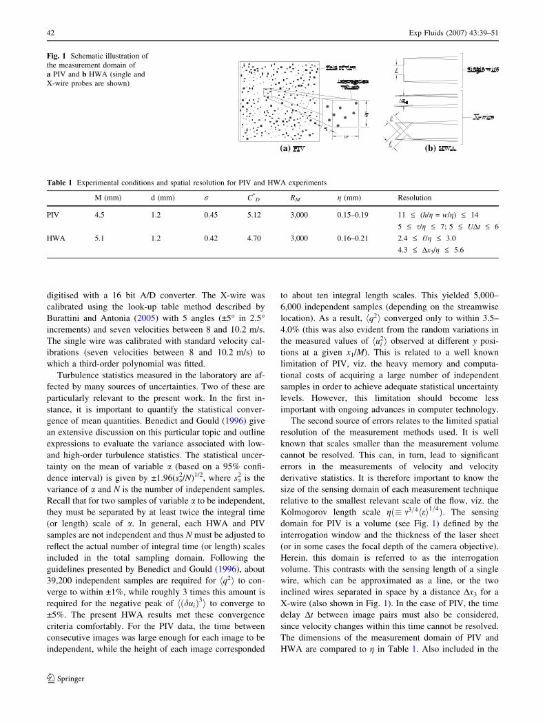
domain for PIV is a volume (see Fig. 1) defined by the

interrogation window and the thickness of the laser sheet

(or in some cases the focal depth of the camera objective).

Herein, this domain is referred to as the interrogation

volume. This contrasts with the sensing length of a single

wire, which can be approximated as a line, or the two

inclined wires separated in space by a distance Dx3 for a

X-wire (also shown in Fig. 1). In the case of PIV, the time

delay Dt between image pairs must also be considered,

since velocity changes within this time cannot be resolved.

The dimensions of the measurement domain of PIV and

HWA are compared to g in Table 1. Also included in the

�

�

�

(a) (b)

Fig. 1 Schematic illustration of

the measurement domain of

a PIV and b HWA (single and

X-wire probes are shown)

Table 1 Experimental conditions and spatial resolution for PIV and HWA experiments

M (mm) d (mm) r C*D RM g (mm) Resolution

PIV 4.5 1.2 0.45 5.12 3,000 0.15–0.19 11 £ (h/g = w/g) £ 14

5 £ s/g £ 7; 5 £ UDt £ 6

HWA 5.1 1.2 0.42 4.70 3,000 0.16–0.21 2.4 £ ‘/g £ 3.0

4.3 £ Dx3/g £ 5.6

42 Exp Fluids (2007) 43:39–51

123

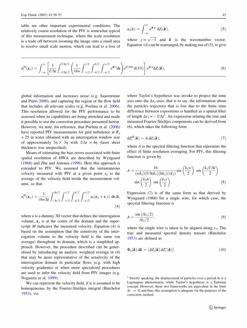
table are other important experimental conditions. The

relatively coarse resolution of the PIV is somewhat typical

of this measurement technique, where the scale resolution

is a trade off between zooming the image onto a small area

to resolve small scale motion, which can lead to a loss of

global information and increases noise (e.g. Saarenrinne

and Piirto 2000), and capturing the region of the flow field

that includes all relevant scales (e.g. Poelma et al. 2006).

This resolution allowed for the PIV performance to be

assessed when its capabilities are being stretched and made

it possible to test the correction procedure presented herein.

However, we note, for reference, that Poelma et al. (2006)

have reported PIV measurements for grid turbulence at Rk

= 25 in water obtained with an interrogation window size

of approximately 3g · 3g with UDt = 4g (laser sheet

thickness was unspecified).

Means of estimating the bias errors associated with finite

spatial resolution of HWA are described by Wyngaard

(1968) and Zhu and Antonia (1996). Here this approach is

extended to PIV. We assumed that the instantaneous

velocity measured with PIV at a given point xo is the

average of the velocity field inside the measurement vol-

ume, so that

uMi xoð Þ ¼

1

shwDt

Z Dt=2

�Dt=2

Z s=2

�s=2

Z h=2

�h=2

Z w=2

�w=2

ui xo þ s; tð Þ ds dt;

ð4Þ

where s is a dummy 3D vector that defines the interrogation

volume, xo is at the centre of the domain and the super-

script M indicates the measured velocity. Equation (4) is

based on the assumption that the sensitivity of the inter-

rogation volume to the velocity field is the same (on

average) throughout its domain, which is a simplified ap-

proach. However, the procedure described can be gener-

alised by introducing an analytic weighted average in (4)

that may be more representative of the sensitivity of the

interrogation domain in particular flows (e.g. with high

velocity gradients) or when more specialised procedures

are used to infer the velocity field from PIV images (e.g.

Nogueira et al. 1999).

We can represent the velocity field, if it is assumed to be

homogeneous, by the Fourier-Stieltjes integral (Batchelor

1953), viz.

ui xð Þ ¼Z 1

�1ejk�x dZi kð Þ; ð5Þ

where j �ffiffiffiffiffiffiffi�1p

and k is the wavenumber vector.

Equation (4) can be rearranged, by making use of (5), to give

where Taylor’s hypothesis was invoke to project the time

axis onto the Dx1-axis; that is to say, the information about

the particles trajectory that is lost due to the finite time

difference between expositions is handled as a spatial filter

of length Dx1 = – UDt1. An expression relating the true and

measured Fourier-Stieltjes components can be derived from

(6), which takes the following form

dZMi kð Þ ¼ A dZi kð Þ; ð7Þ

where A is the spectral filtering function that represents the

effect of finite resolution averaging. For PIV, this filtering

function is given by

A ¼ 16

ðwk1ÞðUDtk1Þðhk2Þðsk3Þsin

k1w

2

� �sin

k1UDt

2

� �

sink2h

2

� �sin

k3s2

� �: ð8Þ

Expression (7) is of the same form as that derived by

Wyngaard (1968) for a single wire, for which case, the

spectral filtering function is

A ¼ sin ‘k3=2ð Þ‘k3=2

; ð9Þ

where the single wire is taken to be aligned along x3. The

true and measured spectral density tensors (Batchelor

1953) are defined as

Uii kð Þ dk ¼ dZi kð Þ dZ�i kð Þ� �

ð10Þ

uMi xoð Þ ¼

Z 1

�1

1

UDt

Z UDt=2

�UDt=2

1

shw

Z s=2

�s=2

Z h=2

�h=2

Z w=2

�w=2

ejk�sds

!

ejUDtk1 d Utð Þ" #

ejk�xdZi kð Þ; ð6Þ

1 Strictly speaking, the displacement of particles over a period Dt is a

Lagrangian phenomenon, while Taylor’s hypothesis is a Eulorian

concept. However, these two frameworks are equivalent in the limit

Dt fi 0, and thus, this assumption is adequate for the purposes of the

correction method.

Exp Fluids (2007) 43:39–51 43

123

UMii kð Þdk ¼ dZM

i kð Þ dZM�i kð Þ

� �; ð11Þ

where the asterisk denotes a complex conjugate. It thus

follows that

UMii kð Þ ¼ A2Uii kð Þ: ð12Þ

The same can be applied to the spectra of the velocity

derivatives hðoui=oxnÞ2i; which yields

UMi;n kð Þ ¼ sin2 Dxnkn=2ð Þ

Dxn=2ð Þ2UM

ii kð Þ; ð13Þ

where Dxn is the distance between each independently

measured values of ui (i.e. values that are obtained from

non-overlapping windows) along the direction xn. This

form of (13) is general and can be applied to any mea-

surement method for which FiiM(k) is known.

Correction ratios for one-dimensional velocity spectra

are defined as

Ruik1ð Þ ¼

/Mui

k1ð Þ/ui

k1ð Þ¼R Rþ1�1 UM

ii kð Þdk2dk3R Rþ1�1 Uii kð Þdk2dk3

; ð14Þ

where the ‘true’ spectra Fij (k) for isotropic turbulence are

given by (e.g. Batchelor 1953)

Uij kð Þ ¼ Uij kð Þ ¼ EðkÞ4pk4

k2dij � kikj

� �; ð15Þ

k is the magnitude of k, E(k) is the 3D energy spectrum and

dij is the Kronecker delta. Similarly, correction coefficients

for the components of the mean turbulent kinetic energy

and vorticity variance are defined as

rui¼

u2i

� �M

u2ih i¼R R Rþ1

�1 UMii kð Þdk1dk2dk3

R R Rþ1�1 Uii kð Þdk1dk2dk3

ð16Þ

rui;n¼

oui=oxnð Þ2D EM

oui=oxnð Þ2D E ¼

R R Rþ1�1 UM

i;n kð Þdk1dk2dk3R R Rþ1

�1 Ui;n kð Þdk1dk2dk3

; ð17Þ

where the true velocity derivative spectra are given by

Ui;n kð Þ ¼ k2nUii kð Þ:

The correction coefficients for velocity and velocity

derivative statistics can be calculated from (12)–(17) with

the spatial filtering function expressed by either (8) or (9),

provided E(k) is known. For the results presented in this

paper, the correction coefficients were calculated using the

3D spectra E(k) obtained from the DNS of HIT by Antonia

and Orlandi (2004). For comparison, Figs. 2 and 3 show

the correction ratios Ruiand correction coefficients rui

and

rui;nestimated for different sensor resolutions. The PIV

results presented in the figures are for a square interroga-

tion window (h = w) with a laser sheet thickness s = h/2,

while Dt is neglected for simplicity. Figure 2 illustrates the

range of scales affected by spatial resolution and shows

that the volume averaging of PIV causes a more significant

attenuation of the spectra at high wavenumbers compared

to a HWA probe with similar sensing dimensions. For

example, the small scales (k1g > 0.5) are more closely

represented by a single hot-wire with ‘ = 8g compared to a

PIV interrogation volume with h = ‘/2. Even when com-

pared to a X-wire probe, which could be argued to average

the velocity over a sensing domain resembling a volume,

the spectral attenuation of PIV is only marginally improved

for the case where the X-wire dimensions are twice that for

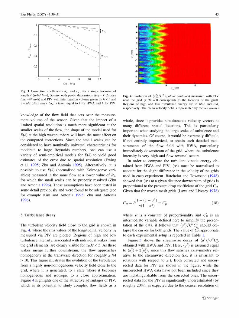
the PIV (Fig. 2). The results presented in Fig. 3 show how

the spectral attenuation of the volume averaging for PIV

affects the integral quantities hu2i i and hðoui=oxnÞ2i: It is

perhaps not surprising that the corrections to these quan-

tities are not as significant for PIV as might be suggested

from Fig. 2, particularly in the case of hu2i i; since most of

the turbulent energy is typically located at scales of the

order of the integral length scale, which is roughly equal to

20g for Rk ~ 40. At such scales, the difference in the ratio

Ruibetween PIV and HWA is much less important. On the

other hand, because hðoui=oxnÞ2i is more heavily weighted

towards the small scales of the flow, the difference in the

correction coefficient rui;nbetween HWA and PIV is larger

than that for rui:

Before concluding this section, it is relevant to discuss

the main drawback of the correction method described

above, viz. the requirement that the velocity spectra be

known a priori. Of course, any method for estimating the

error associated with spatial resolution requires some

Fig. 2 Spectral correction ratio Ruifor PIV at different spatial

resolutions (solid lines); the relative dimensions of the interrogation

volume are assumed to be h = w = 2s. Also included for comparison

are the ratios Ruiði ¼ 1Þ for a single hot-wire (‘ = 8g; dash line) and a

X-wire (‘ = Dx2 = 8g; broken line with dots)

44 Exp Fluids (2007) 43:39–51

123

knowledge of the flow field that acts over the measure-

ment volume of the sensor. Given that the impact of a

limited spatial resolution is much more significant at the

smaller scales of the flow, the shape of the model used for

E(k) at the high wavenumbers will have the most effect on

the computed corrections. Since the small scales can be

considered to have nominally universal characteristics for

moderate to large Reynolds numbers, one can use a

variety of semi-empirical models for E(k) to yield good

estimates of the error due to spatial resolution (Ewing

et al. 1995; Zhu and Antonia 1995). Alternatively, it is

possible to use E(k) (normalised with Kolmogorov vari-

ables) measured in the same flow at a lower value of Rk,

for which the small scales can be properly resolved (Zhu

and Antonia 1996). These assumptions have been tested in

some detail previously and were found to be adequate (see

for example Kim and Antonia 1993; Zhu and Antonia

1996).

3 Turbulence decay

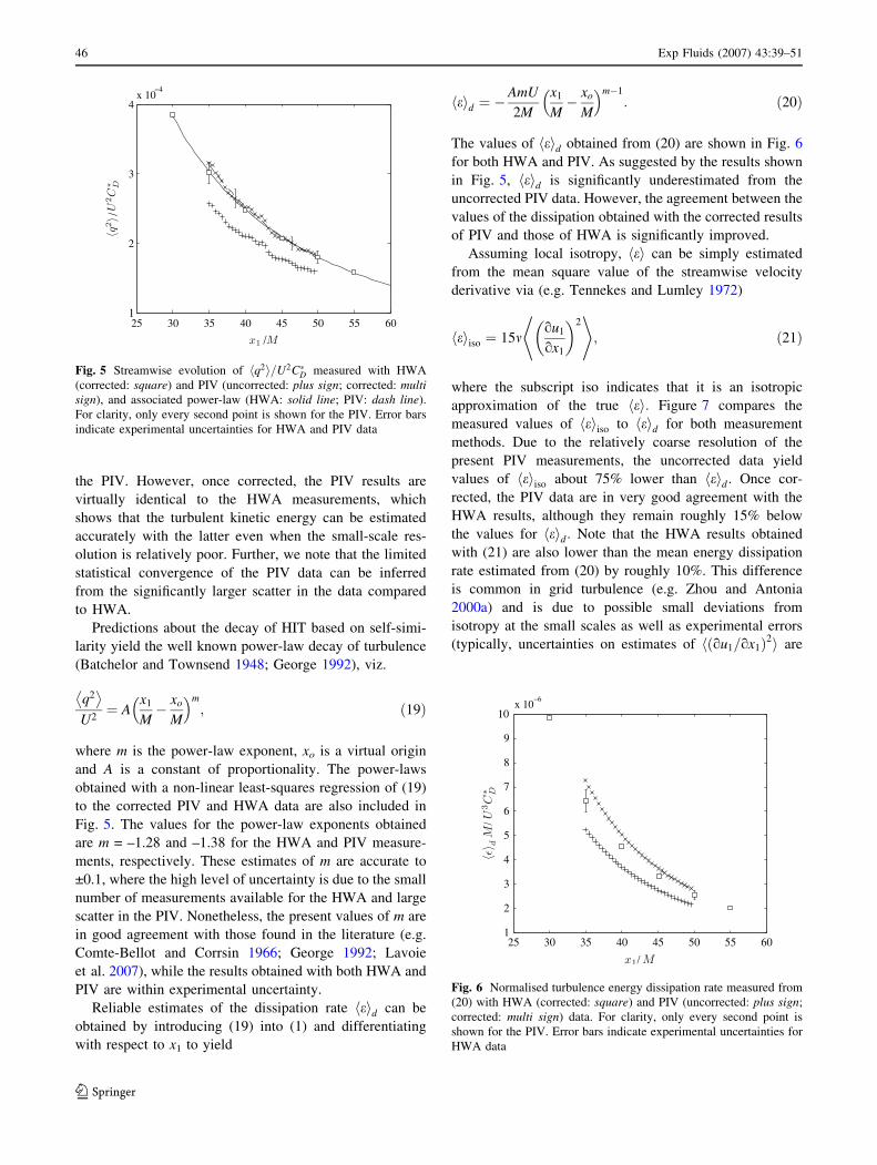
The turbulent velocity field close to the grid is shown in

Fig. 4, where the rms values of the longitudinal velocity u1

measured via PIV are plotted. Regions of high and low

turbulence intensity, associated with individual wakes from

the grid elements, are clearly visible for x1/M < 5. As these

wakes merge further downstream, the flow approaches

homogeneity in the transverse direction for roughly x1/M

> 10. This figure illustrates the evolution of the turbulence

from a highly non-homogeneous velocity field close to the

grid, where it is generated, to a state where it becomes

homogeneous and isotropic to a close approximation.

Figure 4 highlights one of the attractive advantages of PIV,

which is its potential to study complex flow fields as a

whole, since it provides simultaneous velocity vectors at

many different spatial locations. This is particularly

important when studying the large scales of turbulence and

their dynamics. Of course, it would be extremely difficult,

if not entirely impractical, to obtain such detailed mea-

surements of the flow field with HWA, particularly

immediately downstream of the grid, where the turbulence

intensity is very high and flow reversal occurs.

In order to compare the turbulent kinetic energy ob-

tained from HWA and PIV, hq2i must be normalised to

account for the slight difference in the solidity of the grids

used in each experiment. Batchelor and Townsend (1948)

showed that hq2i at a given distance downstream of grids is

proportional to the pressure drop coefficient of the grid CD.

Given that for woven mesh grids (Laws and Livesey 1978)

CD ¼ B1� 1� r2ð Þr 1� r2ð Þ � C�D; ð18Þ

where B is a constant of proportionality and CD* is an

intermediate variable defined here to simplify the presen-

tation of the data, it follows that hq2i=U2C�D should col-

lapse the curves for both grids. The value of CD* appropriate

to each experimental setup is reported in Table 1.

Figure 5 shows the streamwise decay of hq2i=U2C�Dobtained with HWA and PIV. Here, hq2i is assumed equal

to hu21i þ 2hu2

2i; since this flow satisfies axisymmetry rel-

ative to the streamwise direction (i.e. it is invariant to

rotations with respect to x1). Both corrected and uncor-

rected data for PIV are shown in the figure, while the

uncorrected HWA data have not been included since they

are indistinguishable from the corrected ones. The uncor-

rected data for the PIV is significantly underestimated (by

roughly 20%), as expected due to the coarser resolution of

0 2 4 6 8 10 120

0.2

0.4

0.6

0.8

1

Fig. 3 Correction coefficients Ruiand rui;n

for a single hot-wire of

length ‘ (solid line), X-wire with probe dimensions Dx3 = ‘ (brokenline with dots) and PIV with interrogation volume given by h · h and

s = h/2 (dash line). Dxn is taken equal to ‘ for HWA and h for PIV

Fig. 4 Evolution of hu21i=U2 (colour contours) measured with PIV

near the grid (x1/M = 0 corresponds to the location of the grid).

Regions of high and low turbulence energy are in blue and red,

respectively. The mean velocity field is represented by the red arrows

Exp Fluids (2007) 43:39–51 45

123

the PIV. However, once corrected, the PIV results are

virtually identical to the HWA measurements, which

shows that the turbulent kinetic energy can be estimated

accurately with the latter even when the small-scale res-

olution is relatively poor. Further, we note that the limited

statistical convergence of the PIV data can be inferred

from the significantly larger scatter in the data compared

to HWA.

Predictions about the decay of HIT based on self-simi-

larity yield the well known power-law decay of turbulence

(Batchelor and Townsend 1948; George 1992), viz.

q2� �

U2¼ A

x1

M� xo

M

� m

; ð19Þ

where m is the power-law exponent, xo is a virtual origin

and A is a constant of proportionality. The power-laws

obtained with a non-linear least-squares regression of (19)

to the corrected PIV and HWA data are also included in

Fig. 5. The values for the power-law exponents obtained

are m = –1.28 and –1.38 for the HWA and PIV measure-

ments, respectively. These estimates of m are accurate to

±0.1, where the high level of uncertainty is due to the small

number of measurements available for the HWA and large

scatter in the PIV. Nonetheless, the present values of m are

in good agreement with those found in the literature (e.g.

Comte-Bellot and Corrsin 1966; George 1992; Lavoie

et al. 2007), while the results obtained with both HWA and

PIV are within experimental uncertainty.

Reliable estimates of the dissipation rate heid can be

obtained by introducing (19) into (1) and differentiating

with respect to x1 to yield

eh id ¼ �AmU

2M

x1

M� xo

M

� m�1

: ð20Þ

The values of heid obtained from (20) are shown in Fig. 6

for both HWA and PIV. As suggested by the results shown

in Fig. 5, heid is significantly underestimated from the

uncorrected PIV data. However, the agreement between the

values of the dissipation obtained with the corrected results

of PIV and those of HWA is significantly improved.

Assuming local isotropy, hei can be simply estimated

from the mean square value of the streamwise velocity

derivative via (e.g. Tennekes and Lumley 1972)

eh iiso ¼ 15mou1

ox1

� �2* +

; ð21Þ

where the subscript iso indicates that it is an isotropic

approximation of the true hei: Figure 7 compares the

measured values of heiiso to heid for both measurement

methods. Due to the relatively coarse resolution of the

present PIV measurements, the uncorrected data yield

values of heiiso about 75% lower than heid: Once cor-

rected, the PIV data are in very good agreement with the

HWA results, although they remain roughly 15% below

the values for heid: Note that the HWA results obtained

with (21) are also lower than the mean energy dissipation

rate estimated from (20) by roughly 10%. This difference

is common in grid turbulence (e.g. Zhou and Antonia

2000a) and is due to possible small deviations from

isotropy at the small scales as well as experimental errors

(typically, uncertainties on estimates of hðou1=ox1Þ2i are

25 30 35 40 45 50 55 601

2

3

4x 10

−4

/

/

Fig. 5 Streamwise evolution of hq2i=U2C�D measured with HWA

(corrected: square) and PIV (uncorrected: plus sign; corrected: multisign), and associated power-law (HWA: solid line; PIV: dash line).

For clarity, only every second point is shown for the PIV. Error bars

indicate experimental uncertainties for HWA and PIV data

25 30 35 40 45 50 55 601

2

3

4

5

6

7

8

9

10x 10

−6

Fig. 6 Normalised turbulence energy dissipation rate measured from

(20) with HWA (corrected: square) and PIV (uncorrected: plus sign;

corrected: multi sign) data. For clarity, only every second point is

shown for the PIV. Error bars indicate experimental uncertainties for

HWA data

46 Exp Fluids (2007) 43:39–51

123

~10–15%). As mentioned earlier, the present experi-

mental conditions are stretching the ability of the PIV to

resolve the turbulence and it is therefore to be expected

that the small scales should not be adequately captured in

this case—particularly, the uncorrected results. Nonethe-

less, it is encouraging to note that, although the magni-

tude of the PIV corrections is large, the corrected values

are within experimental uncertainties of the corrected

HWA data.

4 Velocity structure functions

In order to compare the longitudinal structure functions

hðdiuiÞni measured with PIV and HWA, these must be

evaluated with separation vectors taken along a direction

where the turbulence is homogeneous. In the case of HWA,

each measurement is separated by a time Dt and Taylor’s

hypothesis is used to give a separation vector r1 (i.e. r1 =

–UDt). For a steady flow, homogeneity along r1 is satisfied

by definition. For PIV, the direction transverse to the mean

flow is homogeneous, so that i = 2 is used for this case.

The second-order longitudinal structure functions

measured at three downstream positions with PIV are

compared with those obtained at x1/M = 45 with HWA in

Fig. 8. The structure functions here are normalised in

accordance with the equilibrium similarity postulate of

George (1992), viz.

diuið Þ2D E

¼ u2i

� �fi erið Þ ð22Þ

� diuið Þ3D E

¼u2

i

� �3=2

Rk

" #

gi erið Þ; ð23Þ

where a tilde represents normalisation with the Taylor

microscale, k ¼ ð15mhu21i=heiÞ

1=2; and Rk ¼ hu21i

1=2k=m is

the Taylor microscale Reynolds number. The inset of

Fig. 8 demonstrates that the structure functions are nearly

independent of the downstream location for the HWA (i.e.

the decay of the turbulence is approximately self-similar).

Although the PIV data are generally lower than the HWA

data at small ~r1; due to spatial resolution effects, they are in

reasonable agreement with each other. It is also important

to note that the structure functions, as obtained by both

methods, are nearly identical in shape, even at large sep-

arations, implying that Taylor’s hypothesis does not have a

strong influence on the shape of these functions—at least in

this flow, where the turbulence intensity is low. (The small

undulations at large ~r for the PIV data are due to the poor

statistical convergence and do not reflect the structure of

the large scales.)

In Fig. 9, the third-order longitudinal structure functions,

divided by ~ri; that were measured with PIV are compared to

those obtained at x1/M = 45 with HWA. The agreement

between HWA and PIV data is not as good as for the sec-

ond-order structure function data. In particular, the peak of

�hðdiuiÞ3i=~ri is greatly underestimated for PIV. This is

perhaps not surprising given that higher order functions are

more sensitive to the spatial resolution. As an illustration,

the inset of Fig. 9 shows results obtained by undersampling

one of the HWA signals in order to mimic a coarser reso-

lution. A sampling frequency N times smaller than fs, where

N is a positive integer, can be simulated by using only every

Nth data point in the original time series. The spatial

averaging of the PIV along x1 can be accounted for when the

velocity at time t is taken as the average of the velocities

25 30 35 40 45 50 55 600

0.2

0.4

0.6

0.8

1/

/

Fig. 7 Ratio heiiso=heid measured with HWA (uncorrected: circle;

corrected: square) and PIV (uncorrected: plus sign; corrected: multisign). For clarity, only every second point is shown for the PIV. Error

bars indicate experimental uncertainties for HWA data

10−1

100

101

0

0.5

1

1.5

2

2.5

1000

1

2

Fig. 8 Second-order structure functions measured with a single

HWA (i = 1: solid line) at x1/M = 45 and PIV (i = 2) at x1/M = 36

(broken line), 41 (dotted line) and 50 (broken line with dots). The

inset compares the functions measured with HWA at x1/M = 35, 45

and 55

Exp Fluids (2007) 43:39–51 47

123

measured over t ± N/fs. This procedure also incorporates

the overlap between interrogation windows, although the

averaging in the x2 and x3 directions due to the interrogation

volume of PIV cannot be included. The curve for N = 5,

which represents an averaging domain of about 11g (similar

to the resolution of the PIV), bears a close resemblance to

the PIV results. Figure 9 demonstrates that for the magni-

tude of the peak in �hðdiuiÞ3i=~ri to be properly determined,

a sensing resolution several times smaller than k, the

approximate location of the peak, is required. This would

represent an interrogation volume smaller than ~(5g)3 for

the present experimental conditions.

Some of the difficulties in evaluating the non-stationary

term in (2) can be alleviated by making use of the fact that

the turbulence decays in an approximately self-similar

manner, as was demonstrated in the inset of Fig. 8. The

similarity form of (2) can then be expressed as (Lavoie

et al. 2005)

gi þ 6f 0i �15Cui1

m� 30Cui2

�~r�4

i ¼ 12~ri; ð24Þ

where the prime denotes differentiation with respect to ~ri;

while Cui1 and Cui2 are given by

Cui1 �Z ~ri

0

~s5f 0i d~s ð25Þ

Cui2 �Z ~ri

0

~s4fid~s: ð26Þ

While the first and second terms on the left-hand side of

(24) represent the non-linear energy transfer and dissipa-

tion rates, respectively, the term in the square brackets ð~IuiÞ

is the non-stationary component due to the streamwise

decay of the turbulence. Each term in (24) was computed

for both the HWA and PIV data and is shown in Fig. 10.

Only one downstream location is shown since similar

results were obtained at other x1/M. Equation (24) is well

balanced at all scales for the HWA data in Fig. 10(a)

(differences between the sums of the terms on the right and

left hand sides are within ±5%). Despite the poor resolution

for the PIV, (24) appears relatively well balanced at all

separations. However, the results of Figs. 8 and 9 suggest

that the energy transfer and dissipation terms in (24) are in

fact significantly underestimated at small separations

ð~ri\2Þ: The apparent balance of the scale-by-scale energy

budget can be accounted for by the behaviour of the non-

stationary term ~Iui; which is shown in Fig. 11. Although the

magnitude of ~Iuiat large values of ~ri is nearly identical for

both measurement techniques, the poor resolution at small

scales for the PIV data causes the term f 0i ð~riÞ in (25) to be

significantly overestimated. The effect of poor spatial res-

olution is further illustrated in the inset of Fig. 11, where

the results obtained by undersampling a HWA signal are

shown. When N is increased, these curves display a similar

100

101

102

0

0.05

0.1

0.15

0.2

100

0

0.05

0.1

0.15

Fig. 9 Third-order structure functions measured with a single HWA

(i = 1: solid line) at x1/M = 45 and PIV i = 2 at x1/M = 36 (brokenline), 41 (dotted line) and 50 (broken line with dots). The inset shows

the result of undersampling the HWA signal obtained at x1/M = 45

with a frequency N times smaller than the actual sampling frequency

10−1

100

101

102

0

2

4

6

8

10

12

14

10−1

100

101

100

2

4

6

8

10

12

14(a)

(b)

/ /

/

/ /

/

Fig. 10 Scale-by-scale energy budget given by (24) and measured

with a a single HWA at x1/M = 45 (i = 1) and b PIV at

x1=M ¼ 41ði ¼ 2Þ:� gi=~ri; solid line; 6f 0i =~ri; broken line; ~Iui=~ri;

broken line with dots; left hand side balance of (23), dotted line. The

thick horizontal line is at 12 (±5%, thick horizontal dash lines)

48 Exp Fluids (2007) 43:39–51

123

trend to that found in the PIV results. The overestimation

of Iuiat small ~ri thus seems to compensate for the over-

estimation of the other terms on the left-hand side of (24).

5 Conclusions

The spatial resolution of HWA and PIV data relative to the

smallest scales of a turbulent flow is an important factor

which can impose considerable limitations on the accuracy

of the measurements in such flows. For the present flow

conditions, the HWA had a resolution roughly 4 times

better than that of PIV (about 2–4g for HWA and 11–14gfor PIV). The results obtained from both measurement

techniques were compared in order to study the effect of

the finite spatial resolution of PIV on turbulence statistics.

The discussion was further supported by the use of an

analytical method—similar to that applied to HWA da-

ta—to account for the effect of finite resolution on PIV

data. The results show that for a PIV interrogation volume

of dimensions equal to a given hot-wire size, the attenua-

tion of the velocity and velocity derivative statistics is

significantly larger for the former, due to the volume

averaging associated with PIV. This assessment of the fi-

nite resolution effects is exclusive of any other sources of

errors associated with either measurement method.

The uncorrected PIV measurements of the turbulent

kinetic energy are significantly underestimated due to poor

spatial resolution. However, even for the stringent condi-

tions designed for this study, the correction method com-

pensates for the attenuation of velocity fluctuations due to

finite resolution. As a result, the corrected PIV results are

in close agreement with the HWA data. Nonetheless, the

spatial resolution of the PIV for the present experimental

conditions is not sufficient to estimate the velocity deriv-

ative statistics with confidence. It is suggested that an

interrogation window of width less than or equal to 5g with

a laser sheet half this dimension in thickness would be

required for the small scale statistics to be estimated with

acceptable accuracy (corrections of less than 30% are re-

quired at this resolution). This dimension is similar to the

resolution that has previously been suggested for hot-wire

arrays (e.g. Zhu and Antonia 1995; Zhou et al. 2003).

The second-order velocity structure functions hðdiuiÞ2imeasured with PIV and HWA are in close agreement with

each other, notwithstanding a slight reduction in the PIV

data arising from the coarser resolution. The lack of sig-

nificant differences in the shape of the structure functions

at large separation suggests that the approximation due to

Taylor’s hypothesis, required to yield hðd1uiÞ2i in the case

of HWA, is not important for this flow where the turbu-

lence intensity is low (<5%). The third-order structure

functions are more sensitive to the limited spatial resolu-

tion of the measurement method and thus display larger

deviations between the two measurement methods. In

particular, the peak magnitude of hðdiuiÞ3i=ri is largely

underestimated by the PIV. This has obvious implications

for PIV-based investigations in the so-called ‘‘scaling

range’’. The agreement between PIV and HWA for the

third-order structure functions is reasonable only at large

separations (r/k > 3, i.e. more than 6 times the PIV reso-

lution). Despite the third-order structure functions being

significantly underestimated, the balance of the scale-by-

scale budget, given by the transport equation of hðdiuiÞ2i; is

fairly good for the PIV. The balance is retrieved due to

errors associated with the non-stationary term, which is

overestimated because of the poor resolution of hðdiuiÞ2iwith respect to ri. It is important to be aware of this limi-

tation since this apparent lack of sensitivity of the scale-

by-scale budget to measurement resolution may lead to an

erroneous interpretation of experimental results.

Overall, this work confirms the relevance of HWA for

studying turbulent flows whilst highlighting the advantages

offered by PIV, such as the availability of simultaneous

velocity measurements at numerous points in space. To

obtain such measurements with HWA would require mul-

tiple sensors that may impose a significant blockage to the

flow. It also illustrates the importance of a number of issues

that need to be considered carefully when designing

experiments. In particular, the spatial resolution should be

selected carefully if all the turbulent scales of interest

(largest and smallest) are to be evaluated correctly. Given a

particular camera resolution, a compromise needs to be

found between an image size large enough to capture the

large scales and an interrogation window small enough to

10−1

100

101

102

0

2

4

6

8

10

12

14

100

102

0

5

10

/

Fig. 11 Comparison of the non-stationary term ~Iuimeasured with a

single HWA (i = 1) at x/M = 45 (solid line) and PIV (i = 2) at x/M= 36 (broken line), 41 (dotted line) and 50 (broken line with dots).

The inset shows the result of undersampling the HWA signal obtained

at x1/M = 45 with a frequency N times smaller than the actual

sampling frequency

Exp Fluids (2007) 43:39–51 49

123

capture the small scales, while still providing an appropriate

signal to noise ratio to minimise the number of spurious

velocity vectors. In addition, given the computational ex-

pense of storing and processing large numbers of PIV

images, statistical tools should be used for optimising the

number of images required to achieve the desired statistical

convergence for the flow parameters of interest. These

issues are not new and have to be handled by researchers

interested in turbulent flows. However, their importance

cannot be understated and warrants constant vigilance by

experimentalists; particularly with the growing availability

of measurement systems in the form of streamlined user

friendly black boxes. Nevertheless, it is encouraging to note

that the typical resolution of current PIV measurements is

constantly improving due to the continuing advances in

technology, and data acquisition and processing techniques.

Acknowledgements We thank Drs. R.J. Smalley and P. Burattini

for many useful discussions. PL and RAA acknowledge the support of

the Australian Research Council.

References

Antonia RA (1993) Direct numerical simulations and hot wire

experiments: a possible way ahead? In: Dracos T, Tsinober A

(eds) New approaches and concepts in turbulence. Birkhauser

Verlag, Basel, pp 349–365

Antonia RA, Orlandi P (2004) Similarity of decaying isotropic

turbulence with a passive scalar. J Fluid Mech 505:123–151

Antonia RA, Zhou T, Zhu Y (1998) Three-component vorticity

measurements in a turbulent grid flow. J Fluid Mech 374:29–57

Antonia RA, Orlandi P, Zhou T (2002) Assessment of a three-

component vorticity probe in decaying turbulence. Exp Fluids

33:384–390

Antonia RA, Smalley RJ, Zhou T, Anselmet F, Danaila L (2003)

Similarity of energy structure functions in decaying homoge-

neous isotropic turbulence. J Fluid Mech 487:245–269

Batchelor GK (1953) The theory of homogeneous turbulence.

Cambridge University Press, London

Batchelor GK, Townsend AA (1947) Decay of vorticity in isotropic

turbulence. Proc R Soc London Ser A 190: 534–550

Batchelor GK, Townsend AA (1948) Decay of isotropic turbulence in

the initial period. Proc R Soc London Ser A 193: 539–558

Benedict LH, Gould RD (1996) Towards better uncertainty estimates

for turbulence statistics. Exp Fluids 22:129–136

Burattini P, Antonia RA (2005) The effect of different X-wire

calibration schemes on some turbulence statistics. Exp Fluids

38:80–89

Comte-Bellot G, Corrsin S (1966) The use of a contraction to improve

the isotropy of grid-generated turbulence. J Fluid Mech 25:657–

682

Corrsin S (1963) Turbulence: experimental methods. In: Fugge S,

Truesdell CA (eds) Handbuch der Physik. Springer, Heidelberg,

pp 524–589

Danaila L, Anselmet F, Zhou T, Antonia RA (1999) A generalisation

of Yaglom’s equation which accounts for the large-scale forcing

in heated decaying turbulence. J Fluid Mech 391:359–372

Ewing D, Hussein HJ, George WK (1995) Spatial resolution of

parallel hot-wire probes for derivative measurements. Exp

Therm Fluid Sci 11:155–173

Foss JF, Wallace JM (1989) The measurement of vorticity in

transitional and fully developed turbulent flows. In: Gad-el-Hak

M (ed) Lecture notes in engineering, vol 45. Springer, Heidel-

berg, pp 263–321

Foucaut JM, Carlier J and Stanislas M (2004) PIV optimization for

the study of turbulent flow using spectral analysis. Meas Sci

Technol 15:1046–1058

Gagne Y, Castaing B, Baudet C, Malecot Y (2004) Reynolds

dependence of third-order structure functions. Phys Fluids

16(2):482–485

George WK (1992) The decay of homogeneous isotropic turbulence.

Phys Fluids 4:1492–1509

George WK, Wang H, Wollbald C, Johansson TG (2001) Homoge-

neous turbulence and its relation to realizable flows. In:

Proceedings of the 14th Australasian fluid mechanics confer-

ence, Adelaide University, pp. 41–48

von Karman T and Howarth L (1938) On the statistical theory of

isotropic turbulence. Proc R Soc London Ser A 164:192–215

Kim J, Antonia RA (1993) Isotropy of the small scales of turbulence

at low Reynolds number. J Fluid Mech 251:219–238

Lavoie P, Burattini P, Djenidi L, Antonia RA (2005) Effect of initial

conditions on decaying grid turbulence at low Rk. Exp Fluids

39:865–874

Lavoie P, Djenidi L, Antonia RA (2007) Effects of initial conditions

in decaying turbulence generated by passive grids. J Fluid Mech

(Accepted for publication)

Laws EM, Livesey JL (1978) Flow through screens. Annu Rev Fluid

Mech 10:247–266

Moin P, Mahesh K (1998) Direct numerical simulation: a tool in

turbulence research. Annu Rev Fluid Mech 30:539–578

Muller E, Nobach H, Tropea C (1998) Model parameter estimation

from non-equidistant sampled data sets at low data rates. Meas

Sci Technol 9:435–441

Mydlarski L, Warhaft Z (1996) On the onset of high-Reynolds-

number grid-generated wind tunnel turbulence. J Fluid Mech

320:331–368

Nogueira J, Lecuona A, Rodriguez PA (1999) Local field correction

PIV: on the increase of accuracy of digital PIV systems. Exp

Fluids 27:107–116

Poelma C, Westerweel J, Ooms G (2006) Turbulence statistics from

optical whole-field measurements in particle-laden turbulence.

Exp Fluids 40: 347–363

Romano GP, Antonia RA, Zhou T (1999) Evaluation of LDA

temporal and spatial velocity structure functions in a low

Reynolds number turbulent channel flow. Exp Fluids 27:368–

377

Saarenrinne P, Piirto M (2000) Turbulent kinetic energy dissipation

rate estimation from PIV velocity vector fields. Exp Fluids

(Suppl) S300–S307

Saffman PG (1968) Lectures on homogeneous turbulence. In:

Zabusky N (ed) Topics in nonlinear physics. Springer, Heidel-

berg, pp 485–614

Saikrishnan N, Marusic I, Longmire EK (2006) Assessment of dual

plane PIV measurements in wall turbulence using DNS data. Exp

Fluids 41:265–278

Scarano F (2003) Theory of non-isotropic spatial resolution in PIV.

Exp Fluids 35:268–277

Sirivat A, Warhaft Z (1983) The effect of a passive cross-stream

temperature gradient on the evolution of temperature variance

and heat flux in grid turbulence. J Fluid Mech 128:323–346

Suzuki Y, Kasagi N (1992) Evaluation of hot-wire measurements in

wall shear turbulence using a direct numerical simulation

database. Exp Therm Fluid Sci 5:69–77

Tennekes H, Lumley JL (1972) A first course in turbulence. MIT

Press, Cambridge

50 Exp Fluids (2007) 43:39–51

123

Van Maanen HRE, Nobach H, Benedict LH (1999) Improved

estimator for the slotted autocorrelation function of randomly

sampled LDA data. Meas Sci Technol 10:L4–L7

Westerweel J, Dabiri D, Gharib M (1997) The effect of a discrete

window offset on the accuracy of cross-correlation analysis of

digital PIV recordings. Exp Fluids 23:20–28

Wyngaard JC (1968) Measurement of small-scale turbulence struc-

tures with hot wires. J Sci Instrum 1:1105–1108

Zhou T, Antonia RA (2000a) Reynolds number dependence of the

small-scale structure of grid turbulence. J Fluid Mech 406:81–

107

Zhou T, Antonia RA (2000b) Approximations for turbulent energy

and temperature variance dissipation rates in grid turbulence.

Phys Fluids 12(2):335–344

Zhou T, Antonia RA, Lasserre J-J, Coantic M, Anselmet F (2003)

Transverse velocity and temperature derivative measurements in

grid turbulence. Exp Fluids 34:449–459

Zhu Y, Antonia RA (1995) Effect of wire separation on X-probe

measurements in a turbulent flow. J Fluid Mech 287: 199–223

Zhu Y, Antonia RA (1996) The spatial resolution of hot-wire arrays

for the measurement of small-scale turbulence. Meas Sci

Technol 7:1349–1359

Exp Fluids (2007) 43:39–51 51

123