sensors

Article

Hardware-in-the-Loop Simulations with Umbra Conditions forSpacecraft Rendezvous with PMD Visual Sensors

Ksenia Klionovska * and Matthias Burri

�����������������

Citation: Klionovska, K.; Burri, M.

Hardware-in-the-Loop Simulations

with Umbra Conditions for Spacecraft

Rendezvous with PMD Visual

Sensors. Sensors 2021, 21, 1455.

https://doi.org/10.3390/s21041455

Received: 13 January 2021

Accepted: 16 February 2021

Published: 19 February 2021

Publisher’s Note: MDPI stays neutral

with regard to jurisdictional claims in

published maps and institutional affil-

iations.

Copyright: © 2021 by the authors.

Licensee MDPI, Basel, Switzerland.

This article is an open access article

distributed under the terms and

conditions of the Creative Commons

Attribution (CC BY) license (https://

creativecommons.org/licenses/by/

4.0/).

German Space Operations Center, German Aerospace Center, Münchener Straße 20, 82234 Weßling, Germany;matthias.burri@dlr.de* Correspondence: ksenia.klionovska@dlr.de

Abstract: This paper addresses the validation of a robust vision-based pose estimation techniqueusing a Photonic Mixer Device (PMD) sensor as a single visual sensor in the close-range phaseof spacecraft rendezvous. First, it was necessary to integrate the developed hybrid navigationtechnique for the PMD sensor into the hardware-in-the-loop (HIL) rendezvous system developedby the German Aerospace Center (DLR). Thereafter, HIL tests were conducted using the EuropeanProximity Operation Simulator (EPOS) with sun simulation and in total darkness. For the futuremissions with an active sensor, e.g., a PMD camera, it could be useful to use only its own illuminationduring the rendezvous phase in penumbra or umbra, instead of additional flash light. In some tests,the rotational rate of the target object was also tuned. Unlike the rendezvous tests in other works,here we present for the first time closed-loop approaches with only depth and amplitude images of aPMD sensor. For the rendezvous tests in the EPOS laboratory, the Argos3D camera was used at therange of 8 to 5.5 meters; the performance showed promising results.

Keywords: PMD sensor; close range rendezvous; hardware-in-the-loop simulations; illuminationconditions

1. Introduction

Autonomous space rendezvous is an important part of On-Orbit Servicing (OOS) andActive Debris Removal (ADR) missions. The demands for these missions are increasingcontinuously due to the high number of non-operational satellites, spent rocket stages andother different pieces of debris [1], which threaten the International Space Station and otheroperational satellites. During OOS and ADR missions, different services can be provided:replacement of failed subsystems, refueling of propellant, replenishment of a spacecraft’scomponents (e.g., batteries or solar arrays), extension of a mission (e.g., software andhardware upgrades) or complete deorbiting of a non-operational space object. OOS andADR mission scenarios consider at least two space objects: a servicer satellite and a targetobject. In order to accomplish aforementioned tasks, the servicer satellite has to approachthe target at close-range. When the target is non-cooperative, there is no information aboutits position and orientation; any patterns and visual markers for the visual navigation areabsent. The target object may tumble, making it more difficult to determine its pose.

Different visual sensors have been tested for rendezvous scenarios. Strengths andweaknesses of these sensor are compared in the literature. Monocular cameras require anexternal source of illumination, but are small in size and have low power consumption. Afull pose estimate is possible because, for rendezvous in space, the scale of the approachedtarget is usually known or can be estimated. Estimations were used for visual navigationin relation to non-cooperative targets by Gaias et al. [2], Sharma et al. [3] and Bennighoffet al. [4]. Lingenauber et al. [5] presented a plenoptic camera for autonomous robotvision during OOS missions at very close range (as close as 2 meters from a satellitemockup). The use of stereo vision allows the tracking [6,7] and the identification [8] of anilluminated non-cooperative target. Yilmaz et al. considered infrared sensors for relative

Sensors 2021, 21, 1455. https://doi.org/10.3390/s21041455 https://www.mdpi.com/journal/sensors

Sensors 2021, 21, 1455 2 of 17

navigation for future ADR missions [9]. The sensitivity to the radiation emitted by thetarget allows operation in darkness, and pose estimation precision is limited by the sensor’sresolution [10]. Active scanning light detection and ranging (LIDAR) sensors have alreadybeen tested for autonomous rendezvous in real space missions [11] and on the ground[12,13]. Operations in darkness are possible, but their size and the moving parts makethem expensive and fragile.

The use of time-of-flight sensors has been presented in the work of Ventura [14]. Theuse of active visual sensors with the Photonic Mixer Device (PMD) technology for the closerendezvous phase is presented in the works of Tzschichholz [15] and Klionovska et al.[16]. Due to the fact that PMD sensors are built using CMOS fabrication technology, theyhad attractive prices years ago, before low cost automotive LIDARs came onto the market.PMD sensor technology has never been used in any real space application before. The lackof moving parts makes it mechanically robust, and as an active sensor it has the potentialto operate in complete darkness. This fact raised an interest in testing it on ground morethoroughly in a closed-loop rendezvous simulation, in order to evaluate the technology forpotential use for future missions.

For a rendezvous with a non-cooperative target, the choice of an appropriate poseestimation technique is relevant to converting raw sensor data into information usable forguidance, navigation, and control systems. Random Sample Consensus (RANSAC) is thestate-of-the-art iterative parameter estimation technique for data with outliers, and it isused for pose estimation with 3D point clouds from LIDARs and stereo vision systems[13,17]. Some simple deterministic methods such as Principal Component Analyses (PCA)and Singular Value Decomposition (SVD) have been used to find the orientation of themain axis of the target in proximity operations in [15,18]. The Iterative Closest Point (ICP)[19,20] algorithm with its different modifications is one of most popular algorithms forpose estimation with 3D point clouds. Feature-based 2D pose estimation techniques withdetection of contours and edges of objects in space are presented in works of Cropp [21],D’Amico [22] and Petit et al. [23]. There are also optical flow methods [24] that considerpixel intensities in the consecutive images, and template-based techniques [25,26]. A recenttrend is the research with Convolutional Neural Network (CNN)-based algorithms for the6D pose estimation of non-cooperative targets using 2D vision systems [27,28].

Without a robust Guidance Navigation and Control system (GNC) [29], an autonomousrendezvous cannot be achieved. Currently, an advanced GNC system is being developedat DLR within the Rendezvous, Inspection, Capture, Detumbling for Orbital Servicing(RICADOS) project [4,30,31]. The hardware-in-the-loop (HIL) simulation allows one to testapproach trajectories, visual optical sensors and image processing algorithms in real timeon the ground with different illumination conditions. The European Proximity OperationsSimulator (EPOS) at DLR is used as a HIL simulator for the final rendezvous phase (startingfrom 20 meters). The Argos3D camera with a PMD sensor is integrated in the EPOS facility.The developed navigation algorithm for the PMD sensor is part of the current GNC system.

The main subject paper is the evaluation of navigation performance in closed-looprendezvous approaches using the PMD sensor as the single visual sensor. Specifically, weevaluate the effects of illumination conditions and the influences of the rotational rate ofthe target on the accuracy and stability of the navigation system. The pose estimation andnavigation techniques developed for the PMD sensor have been described in previouswork [16,32]. Our previous work [32] used various amounts of recorded images for therendezvous simulations. Thus, the output of the navigation system was not fed into thecontrol system. In this paper the processed PMD sensor measurements are used for the real-time control of the approach trajectory. It is a big step forward towards a fully autonomousapproach with PMD measurements.

This paper is organized as follows. Section 2 describes the HIL rendezvous system,the PMD sensor and the applied pose estimation algorithms. We approached a rotatingtarget in total darkness with strong side illumination. We also compared approaches with

Sensors 2021, 21, 1455 3 of 17

different rotational speeds along the principal axis. Section 3 presents the results anddiscussion of the closed-loop rendezvous scenarios, and the conclusions are in Section 4.

2. Materials and Methods

In this section we present the HIL rendezvous system, the characteristics of the PMDsensor in question, short descriptions of the navigation algorithms and the simulationscenario.

2.1. Hardware-In-The-Loop Rendezvous System

The complex HIL rendezvous system used for the experiments consisted of the simu-lation part and the GNC system; see Figure 1. The simulation part consisted of a software-based satellite simulator and the robotic HIL test facility EPOS [33,34] presented in Figure 2.The advanced GNC system included measurements from the PMD sensor, pose estimationalgorithms, a navigation filter and guidance and control functions.

State Servicer (ECI)

Desired Attitude Servicer

(ECI)

Force Cmd Servicer

ECI

Desired Orbit Servicer (ECI)

PMD Sensor

Measurements

Fused Pose

Estimation

Navigation Filter

Guidance Servicer

(ECI)

PID Controller

Orbit Servicer

(ECI)

Simulation

SW

HW

Interface to Satellite Simulator

EPOS

Robot 1 with PMD sensor Robot 2 with target

GNC System

Transformation LVLH to ECI

Pose Target (Sensor Frame)

Figure 1. Illustration of the hardware-in-the-loop rendezvous system.

As shown in Figure 2, the EPOS rendezvous simulator consists of two robots: Robot1 is able to move along a rail system and robot 2 is fixed at the end of the rail system.The mockup of a satellite (target) is mounted on the fixed robot, whereas the other robot(servicer) carries a Argos3D camera with the PMD sensor inside of a white housing.

Let us describe step-by-step the flow of the diagram in Figure 1. PMD sensor imagesof the target object are acquired. At the stage “Fused Pose Estimation”, those images areprocessed to estimate the position and orientation of the non-cooperative target. The blocks“PMD Sensor Measurements” and “Fused Pose Estimation” can freely be substituted withother visual rendezvous sensors and pose estimation techniques. Nevertheless, they arekept constant for the described setup. The noisy measurements are passed through thenavigation filter described in [35], and we get a pose with minimized noise in the EarthCentral Inertial (ECI) system. Following the data flow of Figure 1, the guidance systemcomputes the desired servicer attitude with the output from the navigation filter in block“Guidance Servicer (ECI)”. A Proportional Integral Derivative (PID) controller in the block“PID Controller Orbit Servicer (ECI)” translates this result to the control forces needed tokeep the servicer on the desired trajectory. The satellite simulator, at the stage “Simulation”,

Sensors 2021, 21, 1455 4 of 17

computes the dynamic motion of the servicer and target, and then forwards this data toEPOS. The EPOS robots move relative to one another according to a real-time attitude andorbit dynamics simulation, just as a servicer and target would move in orbit.

Argos 3D-P320 Camera

Robot 1 Robot 2

Figure 2. EPOS facility: on the left, a robot carries a Photonic Mixer Device (PMD) sensor and theone on the right has a mounted mockup of a satellite.

2.2. Argos 3D-P320 Camera

The Bluetechnix (current BECOM) Argos 3D-P320 camera (white camera in Figure 2)contains the PMD sensor. The PMD sensor is a ranging device that provides a depth imagefor every frame. The depth measurement of every pixel is obtained considering the phaseshift between the emitted signal of LEDs and the signal reflected from the target. Thecamera in the current setup has 12 LEDs. For detailed descriptions of the PMD’s operationalprinciple and depth calculation per pixel, please refer to the works of Langmann [36]. Thetechnical characteristics of the current PMD sensor are presented in Table 1.

As shown in Table 1, the resolution of the current PMD sensor inside the Argos3D-P320 camera is relatively small compared with the traditional CMOS image sensorsavailable on the market. Both sensor families use integrated circuits placed inside eachpixel to convert the incoming light into a digital signal. For the depth calculation, a certainamount of electronics is required, resulting in larger pixels. The current generation of PMDsensors can only achieve pixels of ca. 10 microns, whereas the CMOS camera can reach apixel size of 1 micron [37].

Table 1. Technical data of the PMD sensor inside of the Argos 3D-P320 camera.

Parameter Numerical Values

Field of View 28.91 × 23.45 degResolution of the chip 352 × 287 pixelsIntegration time 24 msFrames per second 45Modulated frequencies 5.004 MHz, 7.5 MHz, 10.007 MHz,

15 MHz, 20.013MHz, 25.016 MHz, 30MHzMass 2 kgPower Consumption <25.5W

Sensors 2021, 21, 1455 5 of 17

On top of depth information, the PMD camera provides a co-registered amplitudegray-scaled image. The amplitude image reflects the strength of the signal returned by thetarget. Single examples of depth and amplitude images taken in the EPOS laboratory withstrong side illumination are presented in Figure 3.

The PMD sensor is an active sensor that can operate even in complete darknesswithout any flash light. This is a big advantage for a future mission planning. A depth andan amplitude image in “umbra conditions” in the EPOS laboratory are shown in Figure 4.

When comparing these two pairs of depth and amplitude images with images takenin the presence of illumination in Figure 3 and images taken in total darkness in Figure 4,one can hardly notice any differences. Even so, the images in Figure 3 are a bit more noisythan in Figure 4. This is due to different systematic and non-systematic errors in PMDsensor measurements [38]. There are several methods for error compensation, which areout of scope in this paper.

An accurately calibrated visual camera is a prerequisite for image processing. Likeusual mono- or stereo cameras, the PMD sensor needs to be calibrated. For this work weconsidered the camera calibration process as an estimation of the camera model (intrinsiccalibration) and estimations of the position and orientation of the PMD sensor frame in thecamera housing (hand-eye calibration) with respect to breadboard of robot 1 of Figure 2. TheDLR CalDe and DLR CalLab calibration toolbox [39] has been used during the calibrationprocedure. The step-by-step calibration process of the current Argos 3D-P320 camera isdescribed in this work [40].

mete

rs

0

2

4

6

8

inte

nsity

0

50

100

150

200

250

Figure 3. (Left): Depth image recorded with an additional illumination spot. The colorbar represents distance measuredto the object in meters. (Right): Amplitude image recorded with an additional illumination spot. The colorbar representsintensity in the range from 0 to 225.

mete

rs

0

2

4

6

8

inte

nsity

0

50

100

150

200

250

Figure 4. (Left): Depth image recorded in complete darkness. The colorbar represents distance measured to the object in meters.(Right): Amplitude image recorded in complete darkness. The colorbar represents intensity in the range from 0 to 225.

Sensors 2021, 21, 1455 6 of 17

2.3. Fused Pose Estimation

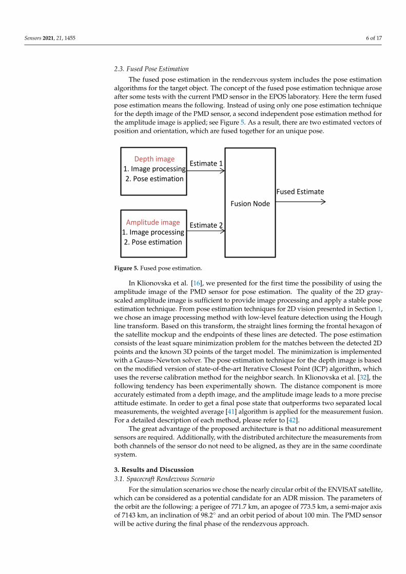
The fused pose estimation in the rendezvous system includes the pose estimationalgorithms for the target object. The concept of the fused pose estimation technique aroseafter some tests with the current PMD sensor in the EPOS laboratory. Here the term fusedpose estimation means the following. Instead of using only one pose estimation techniquefor the depth image of the PMD sensor, a second independent pose estimation method forthe amplitude image is applied; see Figure 5. As a result, there are two estimated vectors ofposition and orientation, which are fused together for an unique pose.

Depth image 1. Image processing 2. Pose estimation

Estimate 1

Estimate 2 Amplitude image 1. Image processing 2. Pose estimation

Fusion Node

Fused Estimate

1

Figure 5. Fused pose estimation.

In Klionovska et al. [16], we presented for the first time the possibility of using theamplitude image of the PMD sensor for pose estimation. The quality of the 2D gray-scaled amplitude image is sufficient to provide image processing and apply a stable poseestimation technique. From pose estimation techniques for 2D vision presented in Section 1,we chose an image processing method with low-level feature detection using the Houghline transform. Based on this transform, the straight lines forming the frontal hexagon ofthe satellite mockup and the endpoints of these lines are detected. The pose estimationconsists of the least square minimization problem for the matches between the detected 2Dpoints and the known 3D points of the target model. The minimization is implementedwith a Gauss–Newton solver. The pose estimation technique for the depth image is basedon the modified version of state-of-the-art Iterative Closest Point (ICP) algorithm, whichuses the reverse calibration method for the neighbor search. In Klionovska et al. [32], thefollowing tendency has been experimentally shown. The distance component is moreaccurately estimated from a depth image, and the amplitude image leads to a more preciseattitude estimate. In order to get a final pose state that outperforms two separated localmeasurements, the weighted average [41] algorithm is applied for the measurement fusion.For a detailed description of each method, please refer to [42].

The great advantage of the proposed architecture is that no additional measurementsensors are required. Additionally, with the distributed architecture the measurements fromboth channels of the sensor do not need to be aligned, as they are in the same coordinatesystem.

3. Results and Discussion3.1. Spacecraft Rendezvous Scenario

For the simulation scenarios we chose the nearly circular orbit of the ENVISAT satellite,which can be considered as a potential candidate for an ADR mission. The parameters ofthe orbit are the following: a perigee of 771.7 km, an apogee of 773.5 km, a semi-major axisof 7143 km, an inclination of 98.2◦ and an orbit period of about 100 min. The PMD sensorwill be active during the final phase of the rendezvous approach.

Sensors 2021, 21, 1455 7 of 17

Using the rendezvous console of the HIL rendezvous system, the straight line approachguidance mode is activated by setting the start (8 meters) and end (5.5 meters) points. Thedistance corresponds to the distance between the centers of mass of the two spacecraft.This limited range span was chosen based on the following factors. The optical power ofthe illumination kit integrated in the PMD sensor restricts the maximum starting point ofthe rendezvous. The minimum distance limit results from the combination of the size ofthe existing mockup, the sensor’s field of view and the pose estimation algorithms thatneed to see the full target. Some points of the detected front hexagon are outside the imagewhen the servicer with the PMD sensor comes closer than 5 meters.

Four test scenarios have been simulated on EPOS; see Table 2. Test I and test IIrepresent approaches with sunlight; the servicer approached the target with illuminationfrom the side. In test III and test IV, the rendezvous tests took place in total darkness tosimulate an approach in umbra conditions. The approach velocity of the servicer in allrendezvous scenarios was 0.01 m/sec. This velocity has proved to be safe for autonomousrendezvous with non-cooperative objects. In test I and test III the target rotated at 3deg/sec; in test II and test IV, 1 deg/sec. These spinning rates were chosen relative toreliably observed rotational rates of ENVISAT satellite in 2012 and 2016 [43]. That madeour test scenarios more realistic. Each test case was repeated and recorded five times.

Table 2. Overview of the test cases.

Case Illumination Target Rotation

Test I Target enlighted 3 deg/secTest II Target enlighted 1 deg/secTest III Umbra conditions 3 deg/secTest IV Umbra conditions 1 deg/sec

We do not consider in this paper a situation where the target object rotates aroundanother axis. However, it should be possible to track a space object by adjusting the fusedpose estimation technique.

3.2. Numerical Results

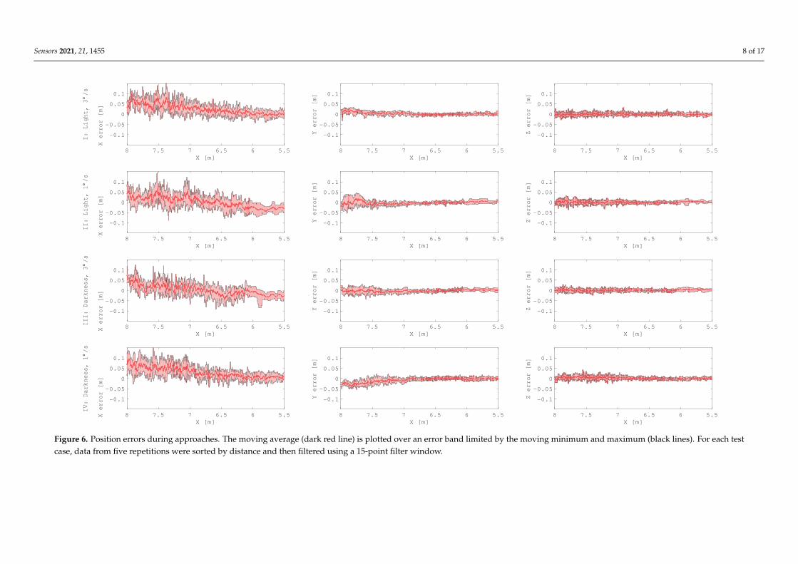
The results were processed in the servicer’s coordinate system. The x axis pointstowards the target. In Figure 6 the position errors of all five approaches in every test caseare presented. For these approach trajectories, the errors for estimation of the distance werequite similar. In most cases the distance was slightly over that estimated; the maximumerror was 16 cm. We observed that with a decreasing distance to the target, the estimatederror dropped and did not exceed 5 cm at the point nearest to the target. The maximumposition error for y and z axes in all test cases was 4.8 cm, but in general it was smaller tothe error for the x axis. If we compare the approaches in total darkness to the approacheswith an illuminated target, we see nearly identical errors. However, approaches in totaldarkness showed a less severe systematic offset. This was expected, since the PMD sensorwas not affected by any illumination or reflected light.

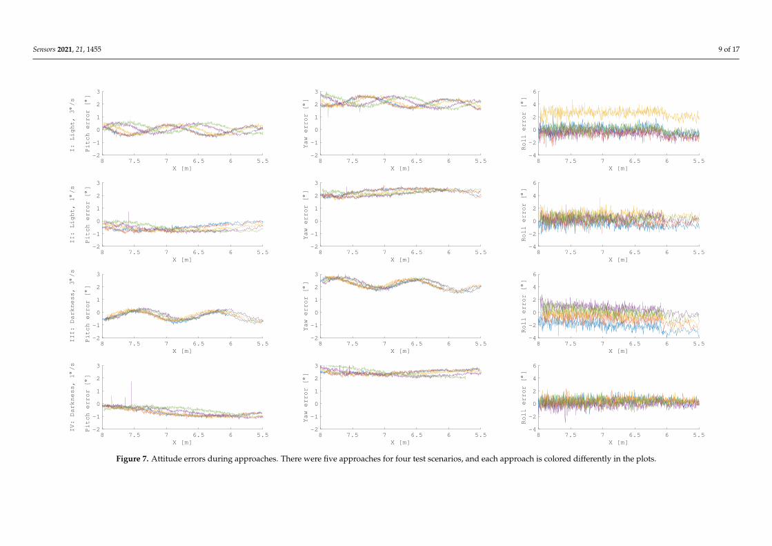
Figure 7 shows the attitude errors. Looking at the plots of the roll angle, it is notdifficult to notice that in test I and test III there were some approaches wherein errorswere higher than in test II and test IV. The angular velocity of a target mockup affectsthe accuracy of the estimated roll angle. All deviations of pitch and yaw angle have asystematic sinusoidal error. The error frequency corresponds to the rotation frequency ofthe target, and the peak to peak amplitude is between 0.36 and 0.88 degrees. In Figure 8,the pitch error is plotted over the yaw error. There is a systematic offset in the yaw anglelarger than 2 degrees. The amplitude and frequency of the systematic errors are similarfor both axis. As a result, the plots for the faster rotating target show circles, whereas theslower rotating target did not complete a full revolution, and therefore, only arc-circles are

Sensors 2021, 21, 1455 8 of 17

5.566.577.58

-0.1

-0.05

0

0.05

0.1

I: Light, 3

°/s

X error [m]

X [m]

5.566.577.58

-0.1

-0.05

0

0.05

0.1

Y error [m]

X [m]

5.566.577.58

-0.1

-0.05

0

0.05

0.1

Z error [m]

X [m]

5.566.577.58

-0.1

-0.05

0

0.05

0.1

III: Darkness, 3

°/s

X error [m]

X [m]

5.566.577.58

-0.1

-0.05

0

0.05

0.1

Y error [m]

X [m]

5.566.577.58

-0.1

-0.05

0

0.05

0.1

Z error [m]

X [m]

5.566.577.58

-0.1

-0.05

0

0.05

0.1

II: Light, 1

°/s

X error [m]

X [m]

5.566.577.58

-0.1

-0.05

0

0.05

0.1

Y error [m]

X [m]

5.566.577.58

-0.1

-0.05

0

0.05

0.1

Z error [m]

X [m]

5.566.577.58

-0.1

-0.05

0

0.05

0.1

IV: Darkness, 1

°/s

X error [m]

X [m]

5.566.577.58

-0.1

-0.05

0

0.05

0.1

Y error [m]

X [m]

5.566.577.58

-0.1

-0.05

0

0.05

0.1

Z error [m]

X [m]

Figure 6. Position errors during approaches. The moving average (dark red line) is plotted over an error band limited by the moving minimum and maximum (black lines). For each testcase, data from five repetitions were sorted by distance and then filtered using a 15-point filter window.

Sensors 2021, 21, 1455 9 of 17

5.566.577.58-2

-1

0

1

2

3

X [m]

I: Light, 3

°/s

Pitch error [

°]

5.566.577.58-2

-1

0

1

2

3

X [m]

Yaw error [

°]

5.566.577.58-4

-2

0

2

4

6

X [m]

Roll error [

°]

5.566.577.58-2

-1

0

1

2

3

X [m]

III: Darkness, 3

°/s

Pitch error [

°]

5.566.577.58-2

-1

0

1

2

3

X [m]

Yaw error [

°]

5.566.577.58-4

-2

0

2

4

6

X [m]

Roll error [

°]

5.566.577.58-2

-1

0

1

2

3

X [m]

II: Light, 1

°/s

Pitch error [

°]

5.566.577.58-2

-1

0

1

2

3

X [m]

Yaw error [

°]

5.566.577.58-4

-2

0

2

4

6

X [m]

Roll error [

°]

5.566.577.58-2

-1

0

1

2

3

X [m]

IV: Darkness, 1

°/s

Pitch error [

°]

5.566.577.58-2

-1

0

1

2

3

X [m]

Yaw error [

°]

5.566.577.58-4

-2

0

2

4

6

X [m]

Roll error [

°]

Figure 7. Attitude errors during approaches. There were five approaches for four test scenarios, and each approach is colored differently in the plots.

Sensors 2021, 21, 1455 10 of 17

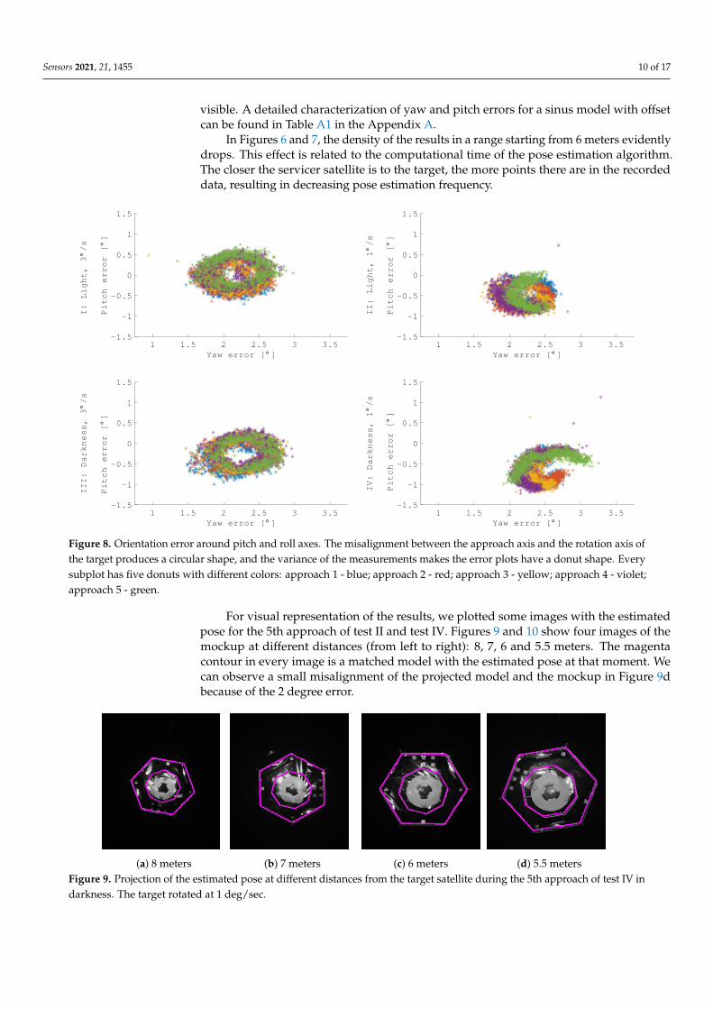
visible. A detailed characterization of yaw and pitch errors for a sinus model with offsetcan be found in Table A1 in the Appendix A.

In Figures 6 and 7, the density of the results in a range starting from 6 meters evidentlydrops. This effect is related to the computational time of the pose estimation algorithm.The closer the servicer satellite is to the target, the more points there are in the recordeddata, resulting in decreasing pose estimation frequency.

1 1.5 2 2.5 3 3.5-1.5

-1

-0.5

0

0.5

1

1.5

Yaw error [° ]

I: Light, 3

°/s

Pitch error [

°]

1 1.5 2 2.5 3 3.5-1.5

-1

-0.5

0

0.5

1

1.5

Yaw error [° ]

III: Darkness, 3

°/s

Pitch error [

°]

1 1.5 2 2.5 3 3.5-1.5

-1

-0.5

0

0.5

1

1.5

Yaw error [° ]

II: Light, 1

°/s

Pitch error [

°]

1 1.5 2 2.5 3 3.5-1.5

-1

-0.5

0

0.5

1

1.5

Yaw error [° ]

IV: Darkness, 1

°/s

Pitch error [

°]

Figure 8. Orientation error around pitch and roll axes. The misalignment between the approach axis and the rotation axis ofthe target produces a circular shape, and the variance of the measurements makes the error plots have a donut shape. Everysubplot has five donuts with different colors: approach 1 - blue; approach 2 - red; approach 3 - yellow; approach 4 - violet;approach 5 - green.

For visual representation of the results, we plotted some images with the estimatedpose for the 5th approach of test II and test IV. Figures 9 and 10 show four images of themockup at different distances (from left to right): 8, 7, 6 and 5.5 meters. The magentacontour in every image is a matched model with the estimated pose at that moment. Wecan observe a small misalignment of the projected model and the mockup in Figure 9dbecause of the 2 degree error.

(a) 8 meters (b) 7 meters (c) 6 meters (d) 5.5 metersFigure 9. Projection of the estimated pose at different distances from the target satellite during the 5th approach of test IV indarkness. The target rotated at 1 deg/sec.

Sensors 2021, 21, 1455 11 of 17

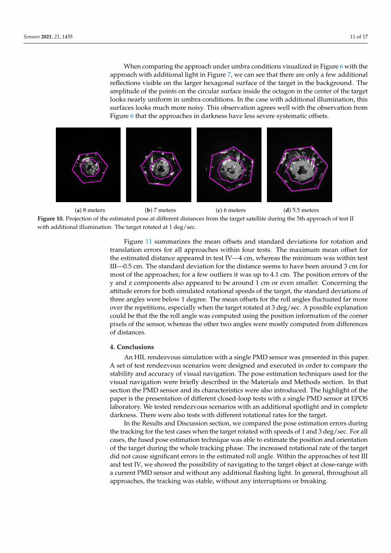
When comparing the approach under umbra conditions visualized in Figure 6 with theapproach with additional light in Figure 7, we can see that there are only a few additionalreflections visible on the larger hexagonal surface of the target in the background. Theamplitude of the points on the circular surface inside the octagon in the center of the targetlooks nearly uniform in umbra conditions. In the case with additional illumination, thissurfaces looks much more noisy. This observation agrees well with the observation fromFigure 6 that the approaches in darkness have less severe systematic offsets.

(a) 8 meters (b) 7 meters (c) 6 meters (d) 5.5 metersFigure 10. Projection of the estimated pose at different distances from the target satellite during the 5th approach of test IIwith additional illumination. The target rotated at 1 deg/sec.

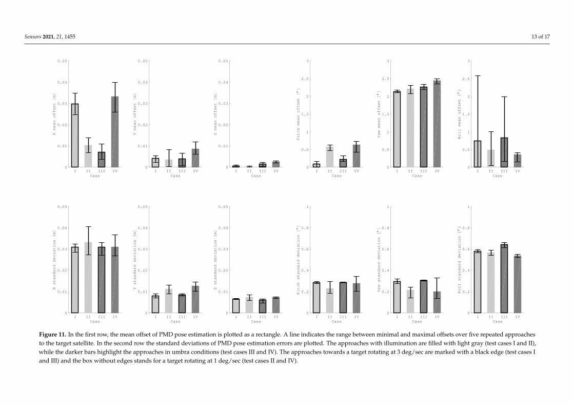
Figure 11 summarizes the mean offsets and standard deviations for rotation andtranslation errors for all approaches within four tests. The maximum mean offset forthe estimated distance appeared in test IV—4 cm, whereas the minimum was within testIII—0.5 cm. The standard deviation for the distance seems to have been around 3 cm formost of the approaches; for a few outliers it was up to 4.1 cm. The position errors of they and z components also appeared to be around 1 cm or even smaller. Concerning theattitude errors for both simulated rotational speeds of the target, the standard deviations ofthree angles were below 1 degree. The mean offsets for the roll angles fluctuated far moreover the repetitions, especially when the target rotated at 3 deg/sec. A possible explanationcould be that the the roll angle was computed using the position information of the cornerpixels of the sensor, whereas the other two angles were mostly computed from differencesof distances.

4. Conclusions

An HIL rendezvous simulation with a single PMD sensor was presented in this paper.A set of test rendezvous scenarios were designed and executed in order to compare thestability and accuracy of visual navigation. The pose estimation techniques used for thevisual navigation were briefly described in the Materials and Methods section. In thatsection the PMD sensor and its characteristics were also introduced. The highlight of thepaper is the presentation of different closed-loop tests with a single PMD sensor at EPOSlaboratory. We tested rendezvous scenarios with an additional spotlight and in completedarkness. There were also tests with different rotational rates for the target.

In the Results and Discussion section, we compared the pose estimation errors duringthe tracking for the test cases when the target rotated with speeds of 1 and 3 deg/sec. For allcases, the fused pose estimation technique was able to estimate the position and orientationof the target during the whole tracking phase. The increased rotational rate of the targetdid not cause significant errors in the estimated roll angle. Within the approaches of test IIIand test IV, we showed the possibility of navigating to the target object at close-range witha current PMD sensor and without any additional flashing light. In general, throughout allapproaches, the tracking was stable, without any interruptions or breaking.

Sensors 2021, 21, 1455 12 of 17

Some further improvements are suggested: Minimization of the PMD sensor’s errors,which affect the final estimated pose of the target. In order to support approaches thatcome closer to the target, the pose estimation algorithm can be improved to work with onlyvisible parts of the target. Replacing the LED illumination unit with laser diodes is anotheroption for the extension of the operational range of the current PMD sensor.

Sensors 2021, 21, 1455 13 of 17

I II III IV0

0.01

0.02

0.03

0.04

0.05

Case

X mean offset [m]

I II III IV0

0.01

0.02

0.03

0.04

0.05

Case

Y mean offset [m]

I II III IV0

0.01

0.02

0.03

0.04

0.05

Case

Z mean offset [m]

I II III IV0

0.5

1

1.5

2

2.5

3

Case

Pitch mean offset [

°]

I II III IV0

0.5

1

1.5

2

2.5

3

Case

Yaw mean offset [

°]

I II III IV0

0.5

1

1.5

2

2.5

3

Case

Roll mean offset [

°]

I II III IV0

0.01

0.02

0.03

0.04

0.05

Case

X standard deviation [m]

I II III IV0

0.01

0.02

0.03

0.04

0.05

Case

Y standard deviation [m]

I II III IV0

0.01

0.02

0.03

0.04

0.05

Case

Z standard deviation [m]

I II III IV0

0.2

0.4

0.6

0.8

1

Case

Pitch standard deviation [

°]

I II III IV0

0.2

0.4

0.6

0.8

1

Case

Yaw standard deviation [

°]

I II III IV0

0.2

0.4

0.6

0.8

1

Case

Roll standard deviation [

°]

Figure 11. In the first row, the mean offset of PMD pose estimation is plotted as a rectangle. A line indicates the range between minimal and maximal offsets over five repeated approachesto the target satellite. In the second row the standard deviations of PMD pose estimation errors are plotted. The approaches with illumination are filled with light gray (test cases I and II),while the darker bars highlight the approaches in umbra conditions (test cases III and IV). The approaches towards a target rotating at 3 deg/sec are marked with a black edge (test cases Iand III) and the box without edges stands for a target rotating at 1 deg/sec (test cases II and IV).

Sensors 2021, 21, 1455 14 of 17

Author Contributions: K.K. and M.B. designed experiments, collected data and collected images;K.K. provided software for the evaluation of pose estimation errors; M.B. contributed with a thoroughanalysis of errors. All authors have read and agreed to the published version of manuscript.

Funding: This research received no external funding.

Institutional Review Board Statement: Not applicable.

Informed Consent Statement: Not applicable.

Data Availability Statement: The data are not publicly available due to the rules of our institute.

Conflicts of Interest: The authors declare no conflict of interest.

AbbreviationsThe following abbreviations are used in this manuscript:

ADR Active Debris RemovalCNN Convolutional Neural NetworksECI Earth Central InertialEPOS European Proximity Operations SimulatorGNC Guidance Navigation and ControlHIL Hardware-in-the-LoopICP Iterative Closest PointLIDAR Light Detection and RangingOOS On-Orbit ServicingPCA Principal Component AnalysesPID Proportional Integral DerivativePMD Photonic Mixer DeviceRANSAC Random Sample ConsensusSVD Singular Value Decomposition

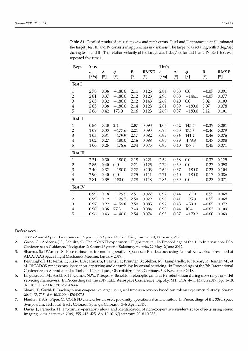
Appendix A. Pitch and Yaw Error Characterization

The pitch and yaw errors plotted in Figures 8 and 7 show a periodical behaviour. Thedata were fitted to the non linear model y(t) = Asin(ωt + φ) + B. The error y is a functionof the time t, the amplitude A, the angular velocity ω, the phase φ and the offset B. Thefit was done using a simplified version of the sinusfit function from this computationalpackage: [44].

The recorded signals used to characterize the error cover less than one period for testsII and IV, and only two periods for tests I and III. Therefore, the present numerical fit is alimit case especially for the frequency estimation. The quality of the result is still enough toclearly separate the cases with a target rotating at 3 deg/sec from the 1 deg/sec angularvelocity cases.

Sensors 2021, 21, 1455 15 of 17

Table A1. Detailed results of sinus fit to yaw and pitch errors. Test I and II approached an illuminatedthe target. Test III and IV consists in approaches in darkness. The target was rotating with 3 deg/secduring test I and III. The rotation velocity of the target was 1 deg/sec for test II and IV. Each test wasrepeated five times.

Rep. Yaw Pitchω A φ B RMSE ω A φ B RMSE[◦/s] [◦] [◦] [◦] [◦] [◦/s] [◦] [◦] [◦] [◦]

Test I

1 2.78 0.36 −180.0 2.11 0.126 2.84 0.38 0.0 −0.07 0.0912 2.81 0.37 −180.0 2.12 0.128 2.96 0.38 −144.1 −0.07 0.0773 2.65 0.32 −180.0 2.12 0.148 2.69 0.40 0.0 0.02 0.1034 2.85 0.38 −180.0 2.14 0.128 2.81 0.39 −180.0 0.07 0.0785 2.86 0.42 173.0 2.16 0.123 2.69 0.37 −180.0 0.12 0.101

Test II

1 0.86 0.48 2.1 2.07 0.098 1.08 0.32 143.3 −0.39 0.0812 1.09 0.33 −177.6 2.21 0.093 0.98 0.33 175.7 −0.46 0.0793 1.05 0.31 −179.9 2.17 0.082 0.99 0.36 141.2 −0.46 0.0764 1.02 0.27 −180.0 2.16 0.088 0.95 0.39 -173.3 −0.47 0.0885 1.00 0.25 −178.6 2.34 0.075 0.95 0.40 177.5 −0.45 0.071

Test III

1 2.31 0.30 −180.0 2.18 0.221 2.54 0.38 0.0 −0.37 0.1252 2.86 0.40 0.0 2.21 0.125 2.74 0.39 0.0 −0.27 0.0903 2.40 0.32 −180.0 2.27 0.203 2.64 0.37 −180.0 −0.23 0.1044 2.90 0.40 0.0 2.25 0.111 2.71 0.40 −180.0 −0.17 0.0865 2.81 0.39 -180.0 2.28 0.118 2.86 0.39 0.0 −0.23 0.071

Test IV

1 0.99 0.18 −179.5 2.51 0.077 0.92 0.44 −71.0 −0.55 0.0682 0.99 0.19 −179.7 2.50 0.079 0.93 0.41 −95.3 −0.57 0.0683 0.97 0.22 −159.8 2.50 0.085 0.92 0.43 −53.0 −0.65 0.0724 0.90 0.36 77.3 2.49 0.084 0.90 0.44 10.4 −0.63 0.1095 0.96 0.43 −146.6 2.54 0.074 0.95 0.37 −179.2 −0.60 0.069

References1. ESA’s Annual Space Environment Report. ESA Space Debris Office, Darmstadt, Germany, 2020.2. Gaias, G.; Ardaens, J.S.; Schultz, C. The AVANTI experiment: Flight results. In Proceedings of the 10th International ESA

Conference on Guidance, Navigation & Control Systems, Salzburg, Austria, 29 May–2 June 2017.3. Sharma, S.; D’Amico, S. Pose estimation for non-cooperative Spacecraft Rendezvous using Neural Networks. Presented at

AIAA/AAS Space Flight Mechanics Meeting, January 2019.4. Benninghoff, H.; Rems, F.; Risse, E.A.; Irmisch, P.; Ernst, I.; Brunner, B.; Stelzer, M.; Lampariello, R.; Krenn, R.; Reiner, M.; et

al. RICADOS-rendezvous, inspection, capturing and detumbling by orbital servicing. In Proceedings of the 7th InternationalConference on Astrodynamics Tools and Techniques, Oberpfaffenhofen, Germany, 6–9 November 2018.

5. Lingenauber, M.; Strobl, K.H.; Oumer, N.W.; Kriegel, S. Benefits of plenoptic cameras for robot vision during close range on-orbitservicing maneuvers. In Proceedings of the 2017 IEEE Aerospace Conference, Big Sky, MT, USA, 4–11 March 2017; pp. 1–18.doi:10.1109/AERO.2017.7943666.

6. Shtark, T.; Gurfil, P. Tracking a non-cooperative target using real-time stereovision-based control: an experimental study. Sensors2017, 17, 735. doi:10.3390/s17040735.

7. Hanlon, E.A.S.; Piper, G. COTS 3D camera for on-orbit proximity operations demonstration. In Proceedings of the 33rd SpaceSymposium, Technical Track, Colorado Springs, Colorado, 3–6 April 2017.

8. Davis, J.; Pernicka, H. Proximity operations about and identification of non-cooperative resident space objects using stereoimaging. Acta Astronaut. 2019, 155, 418–425. doi:10.1016/j.actaastro.2018.10.033.

Sensors 2021, 21, 1455 16 of 17

9. Yilmaz, O.; Aouf, N.; Majewski, L.; Sanchez-Gestido, M.; Ortega, G. Using infrared based relative navigation for active debrisremoval. In Proceedings of the 10th International ESA Conference on Guidance, Navigation & Control Systems, Salzburg, Austria,29 May–2 June 2017.

10. Cassinis, L.; Fonod, R.; Gill, E. Review of the robustness and applicability of monocular pose estimation systems for relativenavigation with an uncooperative spacecraft. Prog. Aerosp. Sci. 2019, 110, 100548. doi:10.1016/j.paerosci.2019.05.008.

11. Cavrois, B.; Vergnol, A.; Donnard, A.; Casiez, P.; Mongrard, O. LIRIS demonstrator on ATV5: a step beyond for european noncooperative navigation system. In Proceedings of the AIAA Guidance, Navigation, and Control Conference, Kissimmee, FL,USA, 5–9 January 2015. doi:10.2514/6.2015-0336.

12. Opromolla, R.; Fasano, G.; Rufino, G.; Grassi, M. Hardware in the loop performance assessment of LIDAR-based spacecraft posedetermination. Sensors 2017, 17, 2197. doi:10.3390/s17102197.

13. Rems, F.; Moreno González, J.A.; Boge, T.; Tuttas, S.; Stilla, U. Fast initial pose estimation of spacecraft from LIDAR point clouddata. In Proceedings of the 13th Symposium on Advanced Space Technologies in Robotics and Automation, Noordwijk, TheNetherlands, 11–13 May 2015.

14. Ventura, J. Autonomous proximity operations for noncooperative space target. Dissertation, Technische Universität München,2016. Available online: https://mediatum.ub.tum.de/doc/1324836/1324836.pdf (accessed on 19 February 2021).

15. Tzschichholz, T. Relative pose estimation of known rigid objects using a novel approach to high-level PMD-/CCD- sensor datafusion with regard to applications in space. Ph.D. Thesis, Universität Würzburg, Würzburg, Germany, 2014. doi:10.25972/OPUS-10391.

16. Klionovska, K.; Ventura, J.; Benninghoff, H.; Huber, F. Close range tracking of an uncooperative target in a sequence of photonicmixer device (PMD) images. Robotics 2018, 7, 5. doi:10.3390/robotics7010005.

17. Schnabel, R.; Wahl, R.; Klein, R. Efficient RANSAC for Point-Cloud Shape Detection. Comput. Graph. Forum 2007, 26, 214–226.doi:j.1467-8659.2007.01016.x.

18. Jasiobedzki, P.; Se, S.; Pan, T.; Umasuthan, M.; Greenspan, M. Autonomous Satellite Rendezvous and Docking using LIDAR andModel Based Vision. Conference: SPIE Spaceborne Sensors II, Orlando, Florida, USA, 2005; Volume 5798. doi:10.1117/12.604011.

19. Woods, J.O.; Christian, J.A. LIDAR-based Relative Navigation with Respect to Noncooperative Objects. Acta Astronaut. 2016, 126,pp. 298-311.

20. Liu, L.; Zhao, G.; Bo, Y. Point Cloud Based Relative Pose Estimation of a Satellite in Close Range. Sensors 2016, 16, 824.doi:10.3390/s16060824.

21. Cropp, A.; Palmer, P. Pose Estimation and Relative Orbit Determination of Nearby Target Microsatellite using Passive Imagery.In Proceedings of the 5th Cranfield Conference on Dynamics and Control of Systems and Structures in Space, Cambridge, UK,14–18 July 2002.

22. D’Amico, S.; Benn, M.; Jorgensen, J.L. Pose Estimation of an Uncooperative Spacecraft from Actual Space Imagery. Int. J. SpaceSci. Eng. 2014, 2, pp.171 - 189. doi:10.1504/IJSPACESE.2014.060600.

23. Petit, A.; March, E.; Kanani, K. Tracking Complex Targets for Space Rendezvous and Debris Removal Applications. In Proceedingsof the IEEE/RSJ International Conference on Intelligent Robots and Systems, IROS’12, Vilamoura-Algarve, Portugal. 7–12 October2012; pp. 4483–4488. doi:10.1.1.394.3774.

24. Pressigout, M.; Marchand, E.; Memin, E. Hybrid Tracking Approach using Optical Flow and Pose Estimation. In Proceedings of the15th IEEE International Conference on Image Processing, San Diego, CA, USA, 12–15 October 2008. doi:10.1109/ICIP.2008.4712356.

25. Opromolla, R.; Fasano, G.; Rufino, G.; Grassi, M. A Model-Based 3D Template Matching Technique for Pose Acquisition of anUncooperative Space Object. Sensors 2015, 15, 6360. doi:10.3390/s150306360.

26. Briechle, K.; Hanebeck, U.D. Template matching using fast normalized cross correlation. In Optical Pattern Recognition XII;Casasent, D.P.; Chao, T.H., Eds.; Society of Photo-Optical Instrumentation Engineers (SPIE) Conference Series; 2001, Volume4387, pp. 95–102. doi:10.1117/12.421129.

27. Sharma, S.; D’Amico, S. Neural Network-Based Pose Estimation for Noncooperative Spacecraft Rendezvous. IEEE Trans. Aerosp.Electron. Syst. 2020, 56, 4638–4658. doi:10.1109/TAES.2020.2999148.

28. Phisannupawong, T.; Kamsing, P.; Torteeka, P.; Channumsin, S.; Sawangwit, U.; Hematulin, W.; Jarawan, T.; Somjit, T.; Yooyen,S.; Delahaye, D.; Boonsrimuang, P. Vision-Based Spacecraft Pose Estimation via a Deep Convolutional Neural Network forNoncooperative Docking Operations. Aerospace 2020, 7, 126. doi:10.3390/aerospace7090126.

29. Risse, E.A.; Schwenk, K.; Bennighoff, H.; Rems, F. Guidance, Navigation and Control for Autonomous Close-Range-Rendezvous.Presented at DLRK online, 2020, DOI: 10.25967/530190.

30. Benninghoff, H.; Rems, F.; Risse, E.A.; Brunner, B.; Stelzer, M.; Krenn, R.; Reiner, M.; Stangl, C.; Gnat, M. End-to-end simulationand verification of GNC and robotic systems considering both space segment and ground segment. CEAS Space J. 2018, 10, pp.535–553. doi:10.1007/s12567-017-0192-2.

31. Rems, F.; Risse, E.A.; Benninghoff, H. Rendezvous GNC-system for autonomous orbital servicing of uncooperative targets. InProceedings of the 10th International ESA Conference on Guidance, Navigation & Control Systems, Salzburg, Austria, 29 May–2June 2017.

32. Klionovska, K.; Benninghoff, H.; Risse, E.A.; Huber, F. Experimental analysis of measurements fusion for pose estimation usingPMD sensor. In Progress in Pattern Recognition, Image Analysis, Computer Vision, and Applications; Vera-Rodriguez, R.; Fierrez, J.;Morales, A., Eds.; Springer International Publishing: Cham, Switzerland , 2019; pp. 401–409. doi:10.1007/978-3-030-13469-3_47.

Sensors 2021, 21, 1455 17 of 17

33. Benninghoff, H.; Rems, F.; Risse, E.A.; Mietner, C. European proximity operations simulator 2.0 (EPOS)-a robotic-basedrendezvous and docking simulator. J. -Large-Scale Res. Facil. 2017, 3, A107. doi:10.17815/jlsrf-3-155.

34. Rems, F.; Bennighoff, H.; Mietner, C.; Risse, E.A.; Burri, M. 10-Year Anniversary of the European Proximity Operations Simulator2.0 - Looking Back at Test Campaigns, Rendezvous Research and Facility Improvements. Presented at DLRK online, 2020.

35. Benninghoff, H.; Rems, F.; Boge, T. Development and hardware-in-the-loop test of a guidance, navigation and control system foron-orbit servicing. Acta Astronaut. 2014, 102, 67–80. doi:10.1016/j.actaastro.2014.05.023.

36. Langmann, B. Wide area 2D/3D Imaging. Development, Analysis and Applications; Springer: Vieweg, Wiesbaden, 2014.doi:10.1007/978-3-658-06457-0.

37. Li, F.; Chen, H.; Pediredla, A.; Yeh, C.; He, K.; Veeraraghavan, A.; Cossairt, O. CS-ToF: high-resolution compressive time-of-flightimaging. Opt. Express 2017, 25, 31096–31110. doi:10.1364/OE.25.031096.

38. Fürsattel, P.; Placht, S.; Balda, M.; Schaller, C.; Hofmann, H.; Maier, A.; Riess, C. A Comparative Error Analysis of CurrentTime-of-Flight Sensors. IEEE Trans. Comput. Imaging 2016, 2, pp. 27–41.

39. Strobl, K.H.; Sepp, W.; Fuchs, S.; Paredes, C.; Smisek, M.; .; Arbter, K. DLR CalDe and DLR CalLab. In Institute of Robotics andMechatronics; German Aerospace Center (DLR): Oberpfaffenhofen, Germany.

40. Klionovska, K.; Benninghoff, H.; Strobl, K.H. PMD Camera-and HandEye-Calibration for On-Orbit Servicing Test Scenarios Onthe Ground. In Proceedings of the In 14th Symposium on Advanced Space Technologies in Robotis and Automation (ASTRA),Leiden, the Netherlands, 20–22 June 2017.

41. Grossman, J.; Grossman, M.; Katz, R. The first Systems of Weighted Differential and Integral Calculus; Archimedes Foundation:Rockport, MA, USA, 1980.

42. Klionovska, K. Analysis and Optimization of PMD-Sensor Data for Rendezvous Applications in Space. Ph.D. Thesis, Universitätder Bundeswehr München, Neubiberg, Germany, 2020. Available online: https://athene-forschung.unibw.de/85311?show_id=134113 (accessed on 19 February 2021).

43. Fraunhofer Institute. Research News. 2017. Available online: https://www.fraunhofer.de/content/dam/zv/en/press-media/2017/August/ResearchNews/rn08_2017_FHR_Defunct%20satellites.pdf (accessed on 19 February 2021).

44. Greene, C.A.; Thirumalai, K.; Kearney, K.A.; Delgado, J.M.; Schwanghart, W.; Wolfenbarger, N.S.; Thyng, K.M.; Gwyther, D.E.;Gardner, A.S.; Blankenship, D.D. The Climate Data Toolbox for MATLAB. Geochem. Geophys. Geosyst. 2019, 20, pp. 3774–3781.doi:10.1029/2019gc008392.