1

Space weather driven changes in lower atmosphere phenomena 1

R.G. Harrison1, K.A. Nicoll

1, K.A. McWilliams

2 2

1Department of Meteorology, University of Reading, UK 3

2Department of Physics and Engineering Physics, University of Saskatchewan, Canada 4

5

Abstract 6

During a period of heliospheric disturbance in 2007-9 associated with a co-rotating interaction 7

region (CIR), a characteristic periodic variation becomes apparent in neutron monitor data. This 8

variation is phase locked to periodic heliospheric current sheet crossings. Phase-locked electrical 9

variations are also seen in the terrestrial lower atmosphere in the southern UK, including an increase 10

in the vertical conduction current density of fair weather atmospheric electricity during increases in 11

the neutron monitor count rate and energetic proton count rates measured by spacecraft. At the 12

same time as the conduction current increases, changes in the cloud microphysical properties lead 13

to an increase in the detected height of the cloud base at Lerwick Observatory, Shetland, with 14

associated changes in surface meteorological quantities. As electrification is expected at the base of 15

layer clouds, which can influence droplet properties, these observations of phase-locked 16

thermodynamic, cloud, atmospheric electricity and solar sector changes are not inconsistent with a 17

heliospheric disturbance driving lower troposphere changes. 18

Keywords 19

Atmospheric electricity; cloud microphysics; co-rotating interaction regions; solar-terrestrial coupling 20

2

1. Introduction 1

Investigating whether space weather can appreciably influence properties and phenomena of the 2

lower atmosphere requires investigation of a complex chain of physical interactions, propagating 3

from the solar wind through high energy charged particles into the magnetosphere and ionosphere, 4

and finally down into the lower troposphere. Although the influence of solar variability on the lower 5

atmosphere is likely to be weak, not least because it lies at the end of the chain of processes, the 6

possibility of coupling of space weather to tropospheric weather has long been recognised as 7

potentially important to the human environment (Ney 1959; Dickinson, 1975). One route through 8

the troposphere is via the global atmospheric electric circuit (Rycroft et al 2000; Rycroft and 9

Harrison, 2011), within which there is a vertical conduction current flowing between the ionosphere 10

and the surface. Recent work (Nicoll and Harrison, 2009, 2010) has confirmed that, as the current 11

passes through layer clouds, charging of their upper and lower boundaries occurs. This could, in 12

principle, modify some of the microphysical interactions between cloud droplets (Rycroft et al 2012, 13

Tinsley, 2008). 14

15

Previous studies have investigated space weather–weather coupling statistically by considering 16

lower atmosphere responses around well-defined marking events, such as solar sector boundary 17

crossings (Wilcox et al 1973; Tinsley and Deen 1991), and Forbush decreases in cosmic rays (e.g. 18

Chronis, 2009). This approach allows reduction of meteorological variability by averaging 19

atmospheric quantities around the marker events. The technique requires that the marker events 20

are abundant, and that there is a good expectation of consistent responses across the different 21

events, as otherwise the results may be sensitive to details of the sampling (Harrison and Ambaum, 22

2010). A disadvantage is that responses which can only be determined in an average sense may not 23

indicate the consequences of individual space weather events or solar changes. An alternative 24

method is to study episodes of well-defined variability in solar parameters, investigating whether a 25

characteristic signature originating in the heliosphere can propagate through a chain of processes 26

into the weather-forming regions of the lower atmosphere. Periods known to have solar-induced 27

oscillatory variation in cosmic rays provide such opportunities (e.g. Harrison 2008), as the flux of 28

galactic cosmic rays (GCR) at Earth varies with the state of the heliosphere. The variation of GCRs is 29

known to influence parameters of atmospheric electricity at the Earth’s surface (Harrison and 30

Usoskin, 2010). 31

32

One solar feature important in determining GCR variability is the existence in interplanetary space of 33

isolated coronal holes, which contribute to shielding within the inner heliosphere. Coronal holes 34

enhance the solar wind outflow and also influence the formation of long-lived solar co-rotating 35

interaction regions (CIRs), ahead of which shock waves and compression regions modulate the 36

cosmic ray fluxes. For late 1996 near solar minimum, Rouillard and Lockwood (2007) showed that an 37

active solar region modulated the GCR flux in this way. This was evident as a well-defined ~27 day 38

oscillation in neutron monitor data from the latter part of 1996, even as observed by eye. Harrison 39

et al (2011) found that a similar oscillation occurred around the beginning of 1997 in surface 40

atmospheric electricity measurements of the Potential Gradient (PG) made in Hungary. 41

42

3

This 1997 CIR-induced variation in PG showed good phase agreement with the Climax neutron 1

monitor data, but, as the amplitude of the PG oscillation was considerably greater than that in the 2

neutron monitor data, it is unlikely that the neutron count rate is directly causally linked to the PG 3

variation, through, for example, ionisation from the primary particles in the upper atmosphere. A 4

further well-defined CIR event was clearly apparent in neutron monitor data around the end of 5

2007, during which changes also occurred in surface atmospheric electricity. These are analysed 6

further here, together with their possible relationship to cloud properties in the lower atmosphere. 7

8

2. Solar changes 9

The regular solar changes considered here arose during late 2007, and are summarised in the panels 10

of data presented in Figure 1. Figure 1(a) shows daily data from the Oulu neutron monitor, in which 11

regular oscillations are straightforwardly apparent, centred on the beginning of 2008. Because of the 12

shorter timescale variability also present, the timings of the maxima and minima of these regular 13

oscillations have been obtained from the maxima and minima remaining after a phase-preserving 14

band pass filter (pass-band 25 to 30 days) was applied to the neutron monitor data, and these 15

positions are also marked in Figure 1(a). 16

Modulation of the neutron monitor data occurs through modulation of galactic cosmic rays which 17

are associated with variations in the interplanetary magnetic field (IMF). The IMF is produced by 18

solar surface magnetic activity and dragged out by the solar wind to interplanetary space. A thin 19

interface between the opposite polarity IMF regions is formed as the heliospheric current sheet. The 20

“Parker spiral” shape (Parker, 1958) of the IMF results from the rotating source of the IMF—the 21

Sun—and the radially expanding solar wind plasma, which is nearly infinitely conducting and carries 22

the IMF with it according to the frozen-flux theorem (Alfvén, 1943). This spinning and expanding 23

“garden hose” effect gives rise to a twisted IMF structure. This structure in the heliospheric current 24

sheet provides dominant sectors of magnetic field “away” (A) or “toward” (T) the Sun, as observed 25

at Earth. Observations have shown periods when the solar sector structure is relatively regular and 26

well-ordered, such as a four-sector structure in the IMF apparent in the original observations (Wilcox 27

and Ness, 1967). 28

29

Orientation changes in the IMF occur abruptly when the heliospheric current sheet is crossed by 30

Earth, resulting in sectors of one dominant IMF orientation between the crossings. Previous studies 31

have shown that the sector boundary crossings are related to changes in the lower atmosphere, 32

such as in atmospheric electricity (Reiter 1977; Burns et al 2006). The maximum in the neutron data 33

occurs at the A/T boundary, and the neutron data minimum occurs at the T/A boundary. To illustrate 34

the relationship of the neutrons to sector boundary crossings, Figure 1(b) shows the solar sector 35

angle, which describes the orientation of the interplanetary magnetic field (IMF) in the solar ecliptic 36

plane. The solar sector angle is calculated using the geocentric solar ecliptic (GSE) coordinate system, 37

where x is directed sunward from Earth, y is in the Earth’s ecliptic plane in the direction opposing the 38

planetary orbit, and z completes the right-handed set. The angle is defined in terms of the IMF B 39

components as the inverse tangent of By/Bx, such that a sector angle of zero is along x. Standard 40

Parker spiral directions at Earth are -45° (“toward” the Sun) and +135° (“away” from the Sun) 41

42

Other measured solar quantities shown in Figure 1 are (c), the total solar irradiance (Fröhlich and 43

Lean, 1998) and (d) the intensity of the Sun’s emission in the ultraviolet, at the Lyman alpha 44

emission line (Woods et al, 2000). In contrast with the solar sector crossing, the emission radiation in 45

the visible (TSI) and at Lyman alpha ultra-violet wavelength do not show close synchronicity with the 46

Oulu neutron monitor data or the solar sector crossings. Consequently, in investigating the possible 47

responses in the Earth’s lower troposphere, we concentrate on electrical changes in the Earth’s 48

atmosphere likely to be influenced directly by energetic particle precipitation. 49

50

4

3. Atmospheric electricity 1

(a) Global circuit 2

Large scale current flow in the lower atmosphere is understood within the conceptual model of the 3

Global atmospheric Electric Circuit (GEC) (Wilson 1921), which represents the surface of the Earth 4

and the lower surface of the ionosphere as two oppositely charged, highly conducting “plates” of a 5

spherical capacitor, with a leaky dielectric (the conductive air) in between. Transfer of positive 6

charge upwards from the top of thunderstorms maintains the positive charge on the ionosphere, 7

and negative charge is transferred down to the surface of the Earth through negative lightning 8

strikes, point discharge currents, and precipitation, through which the ionosphere is electrified to a 9

potential of 250kV more positive than the surface, known as the ionospheric potential, VI. 10

(Rycroft et al 2000 and Aplin et al 2008 give more details on the GEC.) 11

The presence of ions allows the atmosphere to be weakly conducting, hence the potential difference 12

between the ionosphere and the Earth’s surface is associated with a return current, known as the 13

air-Earth conduction current density, Jc, flowing vertically between the ionosphere and the surface at 14

large distances from thunderstorms. Ohm’s law relates Jc to VI and the total resistance, Rc, of the unit 15

area column of air through which it flows from the ionosphere to the surface, by 16

c

I

c

R

VJ = (1). 17

Vertical continuity of Jc between the ionosphere and the Earth’s surface provides a link between the 18

upper atmosphere and the lower troposphere. 19

20

(b) Atmospheric electricity observations at Reading 21

Surface measurements of atmospheric electricity have been made at the Reading University 22

Atmospheric Observatory (RUAO) in the UK (geomagnetic latitude ≈47.5°) since 2006, including the 23

2007-2009 period of interest. Quantities measured at this site include the potential gradient (PG), 24

recorded by an all-weather electric field mill mounted at 2m above the surface, and the total vertical 25

current density. The current density is derived from two horizontal electrodes of different geometry 26

(one corrugated and one flat), as described previously (Bennett and Harrison, 2008), to allow 27

correction for displacement current contributions arising from fluctuations in the PG. For this 28

method to be applied, both collecting electrodes must be functioning, with well-characterised offset 29

corrections. Considerably more data values are available if the collecting electrodes are considered 30

separately and the displacement current correction is regarded as small, such as is the case for 31

steady PG conditions. Against the small disadvantage of neglecting the displacement current, this 32

generates two independent sets of measurements as well as more complete data coverage. 33

Measurements of the current flowing to both the corrugated plate (CP) and flat plate (FP) electrodes 34

were originally made at 1 second resolution, but these values have been averaged to give daily 35

averages. In constructing the daily averages it is important to select conditions in which the 36

atmospheric electrical measurements are not strongly affected by local weather conditions such as 37

precipitation and fog. The PG data were therefore selected on the basis of daily PG between 50-38

200Vm-1

, a range of values found typically in fair weather conditions at RUAO (Harrison, 2011). The 39

criteria on the electrode currents need to be stricter, because of leakage current issues with the 40

apparatus’ insulation during winter conditions. As well as selecting periods when the PG was within 41

the fair weather range, only current measurements made around the early afternoon, between 12-42

15UT were used. Additionally, only values during low wind speed conditions (<2ms-1

) were 43

considered, to minimise effects of blowing space charge, which might otherwise generate 44

appreciable displacement current (or impaction charging) effects. 45

5

The RUAO atmospheric electricity data are shown in Figure 2 during the CIR period from June 2007 1

to May 2008. Figure 2 (a) shows a striking oscillation occurring in the PG at Reading (particularly 2

between 2007.9 and 2008.3), the maxima and minima in which can be seen to be closely linked in 3

phase to the neutron max/min (red and blue lines), and therefore, ultimately, the solar sector 4

boundary crossings. Figure 2 (b) and (c) show data from plate electrodes during the same interval. 5

Much less variability is seen in this data; however, by band-pass filtering using multiple realisations 6

with random in-filling to allow for missing data values, the characteristic 27 day oscillation, showing 7

phase agreement with the neutron monitor data remains. 8

9

Atmospheric electrical responses to solar sector boundary crossings have previously been reported 10

at both polar (Park 1976; Burns et al 2006) and mid-latitudes (Reiter 1977; Fischer and Muhleisen 11

1980). In polar regions, these electrical changes are considered to originate from changes in the 12

ionospheric potential (due to cross polar-cap potential differences) which map downwards to 13

change the surface PG (Burns et al 2006). However, modelling has yet to establish whether such 14

changes couple to the surface electrical parameters at mid-latitudes. 15

16

Figure 3 further demonstrates the phase similarity between the 27 day variations in the Oulu 17

neutron monitor count rates (grey line) and the oscillations in vertical current measured with the 18

independent horizontal plate electrodes at Reading (black points), by compositing the daily 19

measurements for ±14 days around the neutron maximum ((a), (b), (c)) and minimum ((d), (e), (f)) 20

times identified in Figure 1, after removing the outliers apparent in figures 2(b) and (c). The 21

proportional change in current, found by averaging the proportional changes measured separately in 22

the two plate electrodes, shows up to a ±15% variation (Figure 3 (c) and (f)) during each 27 day 23

oscillation period. The phase similarity between the neutron monitor and current data is consistent 24

with modulation of the vertical current at Reading by the incoming GCR flux, however, the amplitude 25

of the neutron change alone is clearly insufficient to account for the measured current variations. 26

27

Whilst neutron monitor data provides a proxy for the GCR flux at the Earth’s surface, the neutrons 28

detected are secondary products of the nucleonic branch of the particle cascade initiated by primary 29

GCRs with energy >1GeV, which may not represent all the modulation of the global circuit occurring, 30

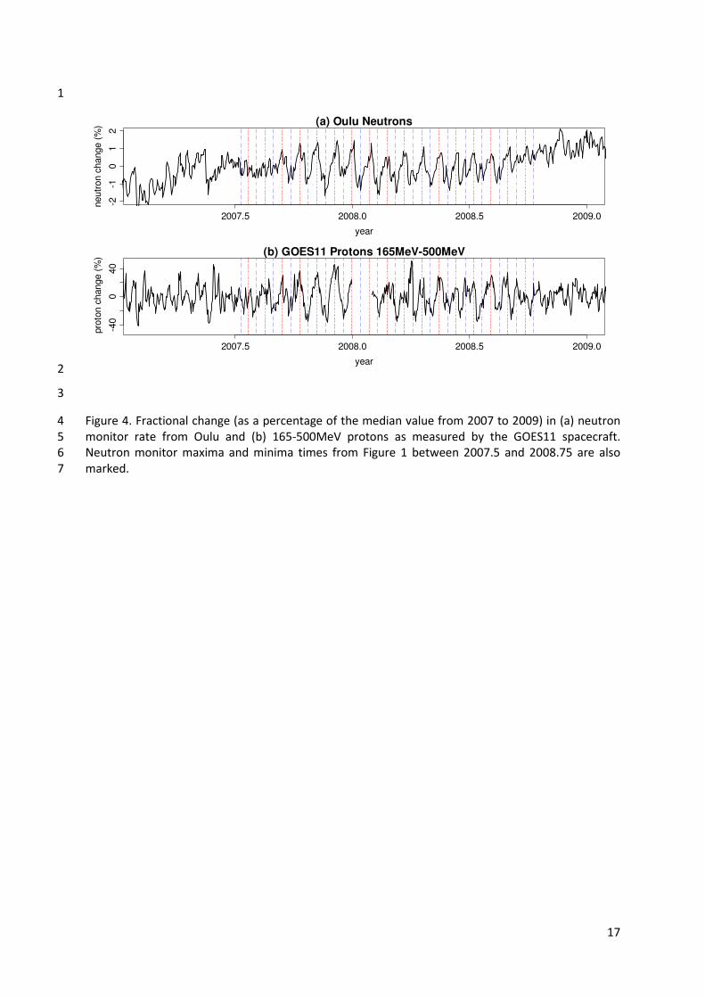
for example in the current generating part of the global circuit. Figure 4 (a) shows the variation in 31

neutron monitor data from Oulu as a percentage of the mean value, demonstrating that the neutron 32

oscillations over the 27 day cycle are at most ±2%, i.e. almost n order of magnitude smaller than the 33

variations in vertical current. Vertical current variations can be up to a few times greater than 34

corresponding neutron monitor variations. For example, a 16% change was found in the vertical 35

current density at Lerwick, Scotland, during an 8% change in neutron monitor count rate between 36

solar maximum and solar minimum; a 30% solar cycle change was also seen in balloon-carried 37

current density measurements made by Olson over Minnesota (Harrison and Usoskin, 2010). One 38

proposed explanation for the difference is that the global atmospheric electric circuit parameters 39

respond to lower energy cosmic rays (<1GeV) than neutron monitors detect. As an example, 40

Figure 4(b) displays the fractional change in the 165-500 MeV protons measured by the GOES 11 41

spacecraft in geosynchronous orbit. These lower energy particles show a much larger proportional 42

variation during the CIR period than the neutron monitor data, of up to ±40%. The 100 MeV protons 43

are sufficiently energetic to create ionisation down to ~32km and 500 MeV particles to 15km in high 44

latitude regions (Bazilevskaya, 2005), and increased ionisation at high altitudes due to the <500 MeV 45

particles will increase the air conductivity, which may influence current flow in the global circuit, 46

contributing additionally to the current modulation at Reading. 47

48

4. Cloud changes 49

(a) Global circuit cloud coupling 50

6

Because the vertical current density shows negligible divergence with height (Rycroft et al 2000), the 1

current density increases associated with the neutron monitor increases shown in Figure 3 are also 2

expected to be characteristic of electrical changes throughout the vertical column. In semi-fair 3

weather regions with fully-overcast layer clouds present, and composed of water droplets 4

(altostratus and stratus clouds), the current in the column will lead to charging at the upper and 5

lower horizontal cloud boundaries (Tinsley 2000; Harrison and Ambaum 2008, 2009), as the current 6

passes through the cloud (Nicoll and Harrison, 2009). For steady meteorological conditions 7

sustaining a persistent sharp horizontal cloud boundary, droplet charging at the upper and lower 8

edges of layer clouds will therefore also vary with the vertical current density. 9

Layer clouds form when ascending moist air cools sufficiently to reach saturation, which depends on 10

the moisture present in the air and the rate at which the temperature falls with height. The height at 11

which the cloud forms is therefore primarily a result of the prevailing meteorological conditions. 12

Following the cloud formation, it is possible that microphysical effects on the cloud droplets may 13

result from their electrification (Rycroft et al, 2012). Since the cloud base is also the cloud boundary 14

charging region, the cloud base is one region which may show particular sensitivity to electrical 15

changes. In general however, investigating any cloud response to current density changes is difficult 16

because of the natural variability usually present in the primary meteorological fluctuations 17

(Harrison and Ambaum, 2010), but, because the neutron monitor variations in 2007-9 show a 18

unusually characteristic form, this period is considered further in meteorological data to study 19

potentially associated cloud responses. 20

(b) Lerwick cloud base 21

Cloud responses to the electrification changes at the lower cloud boundary have previously been 22

investigated using the cloud base height measurements obtained with a laser ceilometer (Harrison 23

et al, 2011). A laser ceilometer operates by timing the transit of an optical pulse travelling between 24

the surface and the cloud base. The position of the zone providing the reflection depends on a 25

combination of droplet size and concentration, and is usually implemented to be associated with a 26

change in visual range, but the exact definition depends on the particular instrument in use. 27

Following Harrison et al (2011), cloud base height data from the Met Office site at Lerwick, Shetland, 28

is considered here for the period of solar variability in 2007-9. This site is frequently cloudy, allowing 29

fluctuations in cloud base to be compared over a sustained period, where electrical and cloud 30

responses have previously been attributed to cosmic ray variations (Harrison and Usoskin 2010, 31

Harrison and Ambaum 2010, Harrison et al 2011). Specifically, the conduction current density at 32

Lerwick, a globally modulated parameter, has been shown to vary positively with the neutron count 33

rate (Harrison and Usoskin, 2010). 34

During the periodic solar changes during 2007-9, automatic cloud base measurements at Lerwick 35

were made consistently with the same Belfort Model C laser ceilometer (Piper, 2011). A time series 36

of the cloud base height data is shown in Figure 5(a), for low cloud base heights, in which variability 37

associated with electrical changes has previously been apparent (Harrison et al 2011). (Figure 5(a) 38

also shows the neutron monitor time series, marked with neutron maxima and minima times as for 39

Figures 1 and 2.) Particularly in 2008, minima in cloud base height are apparent around the neutron 40

minima times, and a positive correlation between neutron count rate and cloud base height is even 41

apparent by eye between 2008.2 and 2008.5. In the surface air temperature measured at the same 42

site, (Figure 5(b)), similar variations can also be identified by eye in the cloud base measurements. 43

As mentioned above, the height at which clouds form depends primarily on the meteorological 44

parameters, such as the local humidity and the rate at which the air temperature falls with height. In 45

surface meteorological measurements, the air temperature Tair and humidity can be represented by 46

the dew point temperature, Tdew, which is the temperature to which the surface air must be cooled 47

to become saturated with respect to water vapour. The dew point depression (Tair-Tdew) is therefore 48

7

zero when the air is saturated, and greater than zero when the air is unsaturated. As a parcel of air 1

cools on ascent its dew point depression also decreases with height if moisture is neither added nor 2

removed, at about 8K km-1

(McIlveen, 1992), although this depends on the local meteorological 3

circumstances. For air at the surface which is unsaturated, this “lapse rate” allows calculation of the 4

height Hcb in metres where the cloud base forms, giving Hcb ~ 125 (Tair-Tdew). The dew point 5

depression therefore provides an additional indication of cloud base height, and, accordingly, the 6

dew point depression measured at Lerwick for the same time interval is shown in Figure 5(c). This 7

also shows a positive correlation with the neutron monitor data during 2008.2 to 2008.4, 8

consistently with the laser cloud base heights. The cloud base height variation observed is therefore 9

not an instrumental artefact of the laser ceilometer. 10

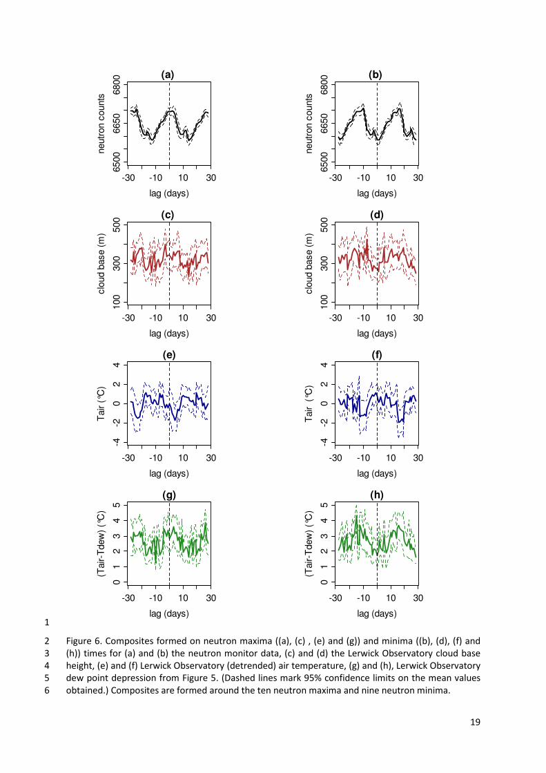
The neutron minima and maxima times are now used to analyse the cloud base height data further. 11

By averaging the cloud base height data around the minima and maxima times, i.e. forming 12

composites, any regular variations occurring will be averaged together. Figure 6 (a) and (b) shows 13

the result of such averaging for the neutron monitor data itself. This procedure makes the form of 14

the neutron maxima and minima distinct, and provides an estimate of the variability associated. 15

Figure 6 (c) and (d) show the same analysis for the cloud base height data. A response in phase with 16

the neutron variation is evident, with some of the smaller features in the neutron data also apparent 17

(e.g. at day +12 in the maxima composite, and day -2 in the minima composite). This is not 18

inconsistent with a symmetric response in the cloud base to increasing and decreasing electrical 19

changes. 20

Figures 6 (e) and (f) show the air temperature measurements as composites formed in the same 21

way. Around the neutron maxima (cloud base raised), the air temperature is reduced, with the 22

opposite response around neutron minima. Consistent responses are again present in composites 23

formed from the dew point depression measurements (Figures 6(g) and (h) ), which estimate a cloud 24

base height increase of ~100m with increasing neutron counts, similar to that observed 25

independently with the laser ceilometer. The variations in cloud base height and dew point 26

depression show close phase agreement with the neutron variations, indicating processes which 27

permit rapid coupling between the heliosphere and lower atmosphere meteorological conditions. 28

To consider the relationship between current density and cloud more quantitatively, Figure 7 shows 29

the proportional changes in current density averaged from both plate electrodes at Reading (already 30

shown in Figure 3) combined with the cloud base height measurements at Lerwick (shown in 31

Figure 6), with both quantities composited on the same neutron maxima. Figure 7(a) shows the 32

temporal variation of the Reading current density and the Lerwick cloud base height, after 33

compositing the values around the neutron maxima. Both quantities increase around the neutron 34

maximum time, which is apparent despite some intermittency in the Reading current density data. 35

Figures 7(b) and (c) show the composite data sets separately, demonstrating the differences 36

between the data from the “inner” weeks (either side of the neutron maximum times), and the 37

“outer” weeks (the next weeks beyond the neutron maximum times, either side of the inner weeks). 38

Both the current density and cloud base height show a reduction between the inner and outer 39

weeks. Using a Mann-Whitney test, the changes in the median cloud base height and current density 40

are statistically significant, with the probabilities p of the changes having arisen by chance p<0.01 41

and p<0.03 respectively. In terms of sensitivity, the median detected cloud base height changes from 42

304m to 273m and the median current changes from 1.7% to -3.5%, or ~ 6m per % change in current 43

density. 44

It should be emphasised that the energetic particles triggering the neutron monitor are not thought 45

to cause the cloud base changes directly, rather that the neutron monitor data, as previously 46

reported by Harrison and Usoskin (2010), indicate conduction current changes are occurring at the 47

Lerwick site. These will pass through pre-existing clouds (Nicoll and Harrison, 2009), formed as a 48

8

result of the local meteorological conditions. The cloud base height fluctuations observed may 1

therefore be associated with charge-influenced cloud microphysical changes at the lower cloud 2

edge, as a consequence of cloud base droplet charging in the vertical current flow. This 3

interpretation would also imply that the dew point depression adjusted in response to the cloud 4

base change. However, because the vertical lapse rate of dew point depression, surface humidity 5

and cloud base height are strongly coupled, the causal relationship cannot be uniquely established. 6

Hence if the cloud base is responding, in part, to the electrical variations as suggested by the 7

observations, it would amount to a perturbation on the background state already established by the 8

local meteorological conditions. 9

10

5. Discussion 11

The sequence of data presented here shows that lower atmosphere meteorological changes show 12

synchronicity with heliospheric changes originating in the effect of solar sector boundary crossings 13

on the interplanetary magnetic field. Relationships between solar sector boundaries and 14

atmospheric electricity have previously been observed in polar (Burns et al, 2006) and mid-latitude 15

regions (Reiter, 1977), and solar sector boundary changes have been suggested to affect weather 16

(Wilcox et al, 1973; Tinsley and Deen, 1991). The previous studies determined effects by averaging 17

over many solar sector boundary crossings, extending over years. In contrast, the effects identified 18

here are apparent directly during marked heliospheric disturbances in 2007-9 due to a co-rotating 19

interaction region. The importance of this is that it generated a distinct variation in neutron monitor 20

data, which, whilst it originated in the abrupt transition of solar sector boundary crossings, showed a 21

smoother periodic form than the boundary crossings also present in other parameters. The clarity of 22

this feature in the neutron monitor data, and in other energetic particles, implies that the similar 23

periodic variations in atmospheric electrical and meteorological data are associated with particle 24

modulation rather than solar radiative changes, in the visible or the ultraviolet. In addition, the lack 25

of phase synchronisation between the radiative data and the electrical and meteorological data is 26

inconsistent with the lower atmosphere effects originating from solar radiative changes. 27

28

The atmospheric electrical data measured at Reading (Figure 2), showed a ±15% variation in the 29

vertical current density (Jc). This can arise from the ionisation of the energetic particles reducing the 30

resistance of the atmospheric column increasing the current density, and/or modulation of the 31

global circuit. Evidence from proton detectors on the GOES-11 satellite is that the 165 MeV to 500 32

MeV proton channels also show substantial modulation synchronous with the neutron monitor 33

modulation, which supports the possibility of a similar variation in protons with energies greater 34

than this (but not measured), but less than the cut-off energy of the Oulu neutron monitor (0.8GeV, 35

which corresponds to ~0.3GeV for protons). 36

37

Conduction current density changes are important as they provide a route by which heliospheric 38

changes can influence layer clouds in the lower atmosphere. Such clouds are important in 39

determining the radiative balance of the planet and atmosphere’s temperature. Composites around 40

the neutron maxima and minima formed from measurements made at Lerwick Observatory show 41

that cloud base, temperature, and dew point depression variations are synchronised with the 42

neutron monitor maxima and minima (Figure 6), but not with the solar radiation changes, which are 43

out of phase with the neutron maxima and minima. This can be understood as arising from changes 44

in cloud base properties, as a result of charging in the cloud base at the cloud/clear air horizontal 45

boundary. The charging in this region is directly proportional to the vertical conduction current. 46

Although there are many possible cloud droplet effects which could be influenced by charge, 47

enhanced droplet electrification would generally act to increase droplet-droplet sticking on collision, 48

even for like-charged droplets (Russell, 1909; Lekner, 2012), reducing the cloud droplet number 49

concentration. The height at which cloud base is detected depends on both the droplet number 50

9

and the droplet size. With increased droplet-droplet sticking, the detected cloud base height level 1

would rise, as the charge-enhanced reduction in droplet number would need to be compensated by 2

an increased time for the droplet size to grow in the cloud updraft by water vapour diffusion. A rise 3

in cloud base would be associated with reduced downward long-wave radiation, and a reduction in 4

air temperature. Such an effect is also apparent in the Lerwick Observatory data (Figure 6), together 5

with an increase in dew point temperature depression which is usually associated with a cloud base 6

height increase. 7

8

9

6. Conclusion 10

Overall, the picture which emerges in the data considered is of solar sector boundaries modulating 11

atmospheric electricity, as has been previously demonstrated by averaging over many events. In the 12

data considered from 2007 to 2009, individual changes can be identified, further clarified by 13

averaging over only a few characteristic events. A simultaneous response in the conduction current 14

of atmospheric electricity occurs, which is known to modify the electrification of layer cloud edges. 15

Any associated cloud base change would lead to a change in air temperature and other local 16

meteorological responses. 17

18

The increase in conduction current density occurs simultaneously with a change in detected cloud 19

base height of about 6m per % conduction current increase. This analysis of daily data is consistent 20

in sign and agrees closely in magnitude with an entirely independent analysis using hourly averaged 21

data of cloud base obtained during polar darkness in both hemispheres (Harrison and Ambaum, 22

2013), which found a sensitivity in the detected cloud base height of 4m per % conduction current 23

change. Although the actual causal chain cannot be uniquely established solely from this lower 24

atmosphere data, the findings are not inconsistent with the inferred conduction current density 25

increase around neutron maxima leading to microphysical changes in the cloud base, in response to 26

which other local meteorological conditions adjust. 27

28

Whilst this period is very unusual in showing such clear signatures in the neutron data, the evidence 29

presented suggests that, not only is surface atmospheric electricity influenced by Space Weather 30

changes, but that weather itself, through cloud, may also be affected. 31

Acknowledgements 32

KAN acknowledges the support of the Leverhulme Trust through an Early Career Fellowship. The 33

research of KAM is supported by a Discovery Grant from the Natural Sciences and Engineering 34

Research Council of Canada. The Oulu neutron measurements were obtained from 35

http://cosmicrays.oulu.fi/ run by Sodankyla Geophysical Observatory. The PMOD solar irradiance 36

data were obtained by the VIRGO Experiment on the cooperative ESA/NASA Mission SOHO, supplied 37

by the World Radiation Centre in Davos and the Lyman-alpha data from the University of Colorado’s 38

Laboratory for Atmospheric and Space Physics. The GOES data were obtained from Space Weather 39

Prediction Center of the National Oceanic and Atmospheric Administration, and the Advanced 40

Composition Explorer (ACE) data from the ACE science center. Luke Barnard assisted with analysis of 41

the energetic particle data. 42

43

10

References 1

Alfvén, H., 1943. On the existence of electromagnetic-hydrodynamic waves, Ark. Mat. Astron. Fys., 2

29, 2, 1–7. 3

4

Aplin, K.L, Harrison, R.G., and Rycroft,M.J., 2008. Investigating Earth’s atmospheric electricity: a role 5

model for planetary studies, Space Sci. Rev., 30, 11-27. 6

7

Bazilevskaya, G., 2005. Solar cosmic rays in the near Earth space and the atmosphere, 8

Adv. Space Res., 35, 458-464. 9

10

Bennett, A.J., and Harrison, R.G., 2008. Surface measurement system for the atmospheric electrical 11

vertical conduction current density, with displacement current correction. J. Atmos. Sol.- Terr. Phys, 12

70, 11-12, 1373-1381. 13

14

Burns G.B., Tinsley, B.A., Klekociuk, A.R., et al, 2006. Antarctic polar plateau vertical electric field 15

variations across heliocentric current sheet crossings, J. Atmos. Sol.- Terr. Phys, 68, 6, 639-654. 16

17

Chronis, T.G., 2009. Investigating possible links between incoming cosmic ray fluxes and lightning 18

activity over the United States, J. Clim., 22, 5748-5745. 19

20

Dickinson, R. E., 1975. Solar variability and the lower atmosphere, Bull. Am. Meterol. Soc. 56, 1240–21

1248. 22

23

Fischer, H.J. and Muhleisen R.P., 1980. The ionospheric potential and the solar magnetic sector 24

boundary crossings, Astronomisches Institut der Universität Tübingen, Aussenstelle, Weissenau. 25 26

Fröhlich, C. and Lean, J. 1998. The sun’s total irradiance: cycles, trends and related climate change 27

uncertainties since 1978. Geophys. Res. Lett. 25, 4377–4380. 28

29

Harrison, R.G., 2008. Discrimination between cosmic ray and solar irradiance effects on clouds, and 30

evidence for geophysical modulation of cloud thickness, Proc Roy Soc Lond A, 464, 2575-2590. 31

32

Harrison, R.G., 2011. Fair Weather Atmospheric Electricity J. Phys.: Conf. Ser. 301 012001. 33

34

Harrison, R.G. and Ambaum, M.H.P., 2008. Enhancement of cloud formation by droplet charging 35

Proc Roy Soc Lond A, 464, 2561-2573. 36

37

Harrison, R.G. and Ambaum, M.H.P. , 2009. Observed atmospheric electricity effect on clouds, 38

Environ. Res. Lett., 4 014003. 39

40

Harrison, R.G. and Ambaum, M.H.P., 2010. Observing Forbush decreases in cloud at Shetland 41

J. Atmos. Sol.- Terr. Phys., 72, 1408-1414. 42

43

Harrison, R.G. and Usoskin, I., 2010. Solar modulation in surface atmospheric electricity J. Atmos 44

Solar-Terr Physics, 72, 176-182. 45

46

Harrison R.G. and Ambaum, M.H.P., 2013. Electrical signature in polar night cloud base variations 47

Environ Res Lett 8 (in press) 48

49

Harrison R.G., Ambaum, M.H.P. and Lockwood,M., 2011. Cloud base height and cosmic rays Proc Roy 50

Soc Lond A, 467, 2777-2791. 51

52

11

Lekner, J., 2012. Electrostatics of two charged conducting spheres, Proc Roy Soc Lond A, 468, 2145, 1

2829-2848. 2

3

McIlveen, R.,1992. Fundamentals of Weather and Climate, 2nd ed, Chapman and Hall, London. 4

5

Nicoll, K.A . and R.G. Harrison, 2009. Vertical current flow through extensive layer clouds J. Atmos 6

Solar-Terr Physics 71, 12, 1219-1221. 7

Nicoll, K.A. and R.G. Harrison, 2010. Experimental determination of layer cloud edge charging from 8

cosmic ray ionisation, Geophys. Res. Lett., 37, L13802, doi:10.1029/2010GL043605 9

10

Ney, E.P., 1959. Cosmic radiation and the weather, Nature, 183, 451-452. 11

12

Park, C.G., 1976. Solar magnetic sector effects on the vertical atmospheric electric field at Vostok 13

Antarctica, Geophys. Res. Lett., 3, 8, 475-478. 14

15

Parker, E.N., 1958. Dynamics of the Interplanetary Gas and Magnetic Fields, Astrophysical Journal, 16

128, 664—676. 17

18

Piper, I., 2011. Private Communication, UK Met Office, Exeter. 19

20

Reiter, R., 1977. The electric potential of the ionosphere as controlled by the solar magnetic sector 21

structure. Result of a study over the period of a solar cycle, J. Atmos. Terr. Phys., 39, 1, 95-99. 22

23

Rouillard, A.P. and Lockwood, M., 2007. The latitudinal effect of co-rotating interaction regions on 24

galactic cosmic rays. Sol. Phys. 245, 191–206. 25

26

Russell, A., 1909. The coefficients of capacity and the mutual attractions or repulsions of two 27

electrified spherical conductors when close together Proc Roy Soc Lond A. 82, 557, 524-531. 28

29

Rycroft, M.J., Israelsson, S. and Price, C., 2000. The global atmospheric electric circuit, solar activity 30

and climate change. J. Atmos. Sol. -Terr. Phys. 62, 1563–1576. 31

32

Rycroft, M.J. and Harrison, R.G., 2011. Electromagnetic atmosphere-plasma coupling: The global 33

atmospheric electric circuit, Space Science Rev 168, 1, 363-384. 34

35

Rycroft, M.J., Nicoll, K.A., Aplin K.L. and Harrison, R.G., 2012. Recent advances in global electric 36

circuit coupling between the space environment and the troposphere, J. Atmos. Sol.-Terr. Phys., 90–37

91, 198–211. 38

39

Tinsley, B.A., and Deen, G.W., 1991. Apparent tropospheric response to MeV-GeV particle flux 40

variations: A connection via electrofreezing of supercooled water in high level clouds?, J. Geophys. 41

Res. 96, 22283–22296. 42

43

Tinsley, B. A., 2000, Influence of solar wind on the global electric circuit, and inferred effects on 44

cloud microphysics, temperature, and dynamics in the troposphere, Space Sci. Rev., 94, 1–2, 231–45

258. 46

47

Tinsley, B.A., 2008, The global atmospheric electric circuit and its effects on cloud microphysics, 48

Rep. Prog. Phys. 71 066801 49

50

12

Wilcox, J.M., and Ness, N.F., 1967. Solar source of the interplanetary sector structure, Solar Physics, 1

1, 3-4, 437—445. 2

3

Wilcox, J.M., Scherrer, P.H., Svalgaard, L., Roberts,W.O., and Olson, R.H., 1973. Solar magnetic sector 4

structure: Relation to circulation of the earth’s atmosphere, Science, 180, 185–186. 5

6

Wilson, C.T.R., 1921. Investigation of lightning discharges and on the electric fields of thunderstorms. 7

Phil. Trans. A, 221, 73-115 8

9

Woods,T.N., Tobiska, W.K., Rottman, G.J., and Worden, J.R. 2000. Improved solar Lyman α irradiance 10

modeling from 1947 through 1999 based on UARS observations, J. Geophys. Res., 105(A12), 27,195–11

27,215, doi:10.1029/2000JA000051 12

13

13

Figure List 1

Figure 1. Time series of solar-influenced parameters. (a) daily average values of Oulu neutron counts 2

(black lines), filtered through a phase-preserving 25-30 day band-pass filter (grey lines). The times of 3

maxima (dashed red lines) and minima (dotted blue lines) values in the filtered waveform around 4

the 2007/8 winter have been identified. (b) Solar sector boundary angles determined from the ACE 5

spacecraft magnetic data. (c) Total solar irradiance (PMOD composite). (d) Composite time series of 6

solar Lyman alpha (121.5nm) emission. 7

8

Figure 2 (a) Daily averages of Reading PG (selected from 5minute observations for those in the fair 9

weather range 50Vm-1

to 200Vm-1

), with the neutron maxima and minima times from figure 1 also 10

marked. (b) Flat plate (FP) and Corrugated plate (CP) electrode current data for low wind speeds 11

(<2ms-1

) only, during which the PG was 50 to 200 Vm-1

, for days having with at least 2hours of data 12

between 12 and 15UT. (On each panel, the grey line shows the bandpass filtered values, plotted on 13

the right-hand y-axis.) 14

15

Figure 3. Anomalies in Flat Plate (FP) current, Corrugated Plate (CP) current, and their combined 16

averaged proportional change, for ±14 days around the maximum (a), (b), (c) and minimum (d),(e) 17

(f), times identified in Figure 1. Values are medians for which there are three days or more each 18

having at least two hours of measurements, within the range 0 to 2.5pA for the Flat Plate and 0 to 19

1.5 pA for the Corrugated Plate. Error bars on (c) and (f) are one standard error on the median. The 20

solid grey line is the averaged anomaly in the neutron monitor count rate for the same times (scale 21

on right-hand axis). 22

23

Figure 4. Fractional change (as a percentage of the median value from 2007 to 2009) in (a) neutron 24

monitor rate from Oulu and (b) 165-500MeV protons as measured by the GOES11 spacecraft. 25

Neutron monitor maxima and minima times from Figure 1 between 2007.5 and 2008.75 are also 26

marked. 27

28

Figure 5. Meteorological data from Lerwick Observatory, Shetland. (a) Daily averaged cloud base 29

height for low cloud base (100m to 600m) (brown lines, left-hand axis). (b) Daily average air 30

temperature (seasonally detrended). (c) Daily dew point depression temperature. Both quantities in 31

(a) and (b) are over-plotted on Oulu neutron monitor data (grey lines, right-hand axis). Neutron 32

maxima and minima times from Figure 1 between 2007.75 and 2008.45 are also marked. 33

34

Figure 6. Composites formed on neutron maxima ((a), (c) , (e) and (g)) and minima ((b), (d), (f) and 35

(h)) times for (a) and (b) the neutron monitor data, (c) and (d) the Lerwick Observatory cloud base 36

height, (e) and (f) Lerwick Observatory (detrended) air temperature, (g) and (h), Lerwick Observatory 37

dew point depression from Figure 5. (Dashed lines mark 95% confidence limits on the mean values 38

obtained.) Composites are formed around the ten neutron maxima and nine neutron minima. 39

40

Figure 7. Comparisons of composites of daily average current density at Reading (black points and 41

lines) averaged from both electrode plates as for Figure 3, and cloud base height at Lerwick (grey 42

points and lines) around the neutron maxima from 2007.75 to 2008.45 as for Figure 5. (a) Temporal 43

variations of current density (black points, left-hand axis) and cloud base (grey points, right-hand 44

axis), with error bars of one standard error. (b) Box plot of daily averages of Lerwick cloud base, 45

divided into the two weeks around the neutron maxima times (inner weeks of lags from days -7 to 46

14

+6) and the outer weeks (lags from days -8 to -14 and 7 to 14), showing medians (thick lines), inter-1

quartile range (box) and outliers marked. (c) As for (b) but for Reading current density. (In both (b) 2

and (c) the points have been randomly horizontally displaced for clarity.) 3

4

Figure 1. Time series of solar-influenced parameters. (a) daily average values of Oulu neutron counts 5

(black lines), filtered through a phase-preserving 25-30 day band-pass filter (grey lines). The times of 6

maxima (dashed red lines) and minima (dotted blue lines) values in the filtered waveform around 7

the 2007/8 winter have been identified. (b) Solar sector boundary angles determined from the ACE 8

spacecraft magnetic data. (c) Total solar irradiance (PMOD composite). (d) Composite time series of 9

solar Lyman alpha (121.5nm) emission. 10

2007.0 2007.5 2008.0 2008.5 2009.0

650

06

650

68

00

ne

utro

ns (

co

un

ts)

(a)

2007.0 2007.5 2008.0 2008.5 2009.0

secto

r a

ng

le (

°)

-18

00

18

0 (b)

2007.0 2007.5 2008.0 2008.5 2009.013

65

.013

65

.313

65

.6

TS

I (W

m−2)

(c)

2007.0 2007.5 2008.0 2008.5 2009.0

3.4

3.6

3.8

ph

oto

ns (1

011cm

−2s

−1) (d)

15

1

Figure 2 (a) Daily averages of Reading PG (selected from 5minute observations for those in the fair 2

weather range 50Vm-1

to 200Vm-1

), with the neutron maxima and minima times from figure 1 also 3

marked. (b) Flat plate (FP) and Corrugated plate (CP) electrode current data for low wind speeds 4

(<2ms-1

) only, during which the PG was 50 to 200 Vm-1

, for days having with at least 2 hours of data 5

between 12 and 15UT. (On each panel, the grey line shows the bandpass filtered values, plotted on 6

the right-hand y-axis.) 7

8

2007.6 2007.8 2008.0 2008.2 2008.4

50

100

150

200

PG

(V

m−1)

-10

-50

510

(a)

2007.6 2007.8 2008.0 2008.2 2008.4

0.0

1.0

2.0

3.0

iFP

(pA

)

-0.1

00.0

00.1

0

(b)

2007.6 2007.8 2008.0 2008.2 2008.4

0.0

1.0

2.0

3.0

iCP

(pA

)

-0.1

5-0

.05

0.0

50.1

5

(c)

16

1

Figure 3. Anomalies in Flat Plate (FP) current, Corrugated Plate (CP) current, and their combined 2

averaged proportional change, for ±14 days around the maximum (a), (b), (c) and minimum (d),(e) 3

(f), times identified in Figure 1. Values are medians for which there are three days or more each 4

having at least two hours of measurements, within the range 0 to 2.5pA for the Flat Plate and 0 to 5

1.5 pA for the Corrugated Plate. Error bars on (c) and (f) are one standard error on the median. The 6

solid grey line is the averaged anomaly in the neutron monitor count rate for the same times (scale 7

on right-hand axis). 8

-0.3

-0.1

0.1

0.3

days from max

FP

change (

pA

)

-14 -7 0 7 14

-50

050

(a)

-0.3

-0.1

0.1

0.3

days from min

FP

change (

pA

)

-14 -7 0 7 14

-50

050

(d)

-0.3

-0.1

0.1

0.3

days from max

CP

change (

pA

)

-14 -7 0 7 14

-50

050

(b)

-0.3

-0.1

0.1

0.3

days from min

CP

change (

pA

)

-14 -7 0 7 14

-50

050

(e)

-20

-10

010

20

days from max

curr

ent change (

%)

-14 -7 0 7 14

-50

050

(c)

-20

-10

010

20

days from min

curr

ent change (

%)

-14 -7 0 7 14

-50

050

(f)

Neutron change (counts)

Neutron change (counts)

Neutron change (counts)

Neutron change (counts)

Neutron change (counts)

Neutron change (counts)

17

1

2

3

Figure 4. Fractional change (as a percentage of the median value from 2007 to 2009) in (a) neutron 4

monitor rate from Oulu and (b) 165-500MeV protons as measured by the GOES11 spacecraft. 5

Neutron monitor maxima and minima times from Figure 1 between 2007.5 and 2008.75 are also 6

marked. 7

2007.5 2008.0 2008.5 2009.0

-2-1

01

2

year

neutr

on c

hange (

%) (a) Oulu Neutrons

2007.5 2008.0 2008.5 2009.0

-40

040

year

pro

ton c

hange (

%)

(b) GOES11 Protons 165MeV-500MeV

18

1

2

Figure 5. Meteorological data from Lerwick Observatory, Shetland. (a) Daily averaged cloud base 3

height for low cloud base (100m to 600m) (brown lines, left-hand axis). (b) Daily average air 4

temperature (seasonally detrended). (c) Daily dew point depression temperature. Both quantities in 5

(a) and (b) are over-plotted on Oulu neutron monitor data (grey lines, right-hand axis). Neutron 6

maxima and minima times from Figure 1 between 2007.75 and 2008.45 are also marked. 7

8

2007.6 2007.8 2008.0 2008.2 2008.4 2008.6

020

040

060

0

clo

ud

ba

se

(m

)

655

06

65

06

750

2007.6 2007.8 2008.0 2008.2 2008.4 2008.6

(a)

2007.6 2007.8 2008.0 2008.2 2008.4 2008.6

62

-2-6

Ta

ir (

°C)

65

50

66

50

675

0(b)

2007.6 2007.8 2008.0 2008.2 2008.4 2008.6

02

46

8

(Ta

ir - T

de

w)

(°C

)

65

50

66

50

675

0(c)

19

1

Figure 6. Composites formed on neutron maxima ((a), (c) , (e) and (g)) and minima ((b), (d), (f) and 2

(h)) times for (a) and (b) the neutron monitor data, (c) and (d) the Lerwick Observatory cloud base 3

height, (e) and (f) Lerwick Observatory (detrended) air temperature, (g) and (h), Lerwick Observatory 4

dew point depression from Figure 5. (Dashed lines mark 95% confidence limits on the mean values 5

obtained.) Composites are formed around the ten neutron maxima and nine neutron minima. 6

-30 -10 10 30

6500

6650

6800

lag (days)

neutr

on c

ounts

(a)

-30 -10 10 30

6500

6650

6800

lag (days)

neutr

on c

ounts

(b)

-30 -10 10 30

100

300

500

lag (days)

clo

ud b

ase (

m)

(c)

-30 -10 10 30100

300

500

lag (days)

clo

ud b

ase (

m)

(d)

-30 -10 10 30

-4-2

02

4

lag (days)

Tair (

°C)

(e)

-30 -10 10 30

-4-2

02

4

lag (days)

Tair (°

C)

(f)

-30 -10 10 30

01

23

45

lag (days)

(Tair-T

dew

) (°

C)

(g)

-30 -10 10 30

01

23

45

lag (days)

(Tair-T

dew

) (°

C)

(h)

20

1

21

1

Figure 7. Comparisons of composites of daily average current density at Reading (black points and 2

lines) averaged from both electrode plates as for Figure 3, and cloud base height at Lerwick (grey 3

points and lines) around the neutron maxima from 2007.75 to 2008.45 as for Figure 5. (a) Temporal 4

variations of current density (black points, left-hand axis) and cloud base (grey points, right-hand 5

axis), with error bars of one standard error. (b) Box plot of daily averages of Lerwick cloud base, 6

divided into the two weeks around the neutron maxima times (inner weeks of lags from days -7 to 7

+6) and the outer weeks (lags from days -8 to -14 and 7 to 14), showing medians (thick lines), inter-8

quartile range (box) and outliers marked. (c) As for (b) but for Reading current density. (In both (b) 9

and (c) the points have been randomly horizontally displaced for clarity.) 10

lag (days)

curr

ent

change

-10%

0%

10%

-14 -7 0 7 14

(a)

250

300

350

220

260

300

340

(b)

clo

ud b

ase h

eig

ht

(m)

outer lags inner lags

(c)

curr

ent

change

outer lags inner lags

-10%

0%

10%