1

Space-efficient Online Approximation of TimeSeries Data: Streams, Amnesia, and Out-of-order

Sorabh Gandhi, Luca Foschini, Subhash SuriDepartment of Computer Science

UC Santa Barbarasorabh, foschini, suri@cs.ucsb.edu

Abstract— In this paper, we present an abstract frameworkfor online approximation of time-series data that yields a unifiedset of algorithms for several popular models: data streams,amnesic approximation, and out-of-order stream approximation.Our framework essentially develops a popular greedy methodof bucket-merging into a more generic form, for which we canprove space-quality approximation bounds. When specialized topiecewise linear bucket approximations and commonly used errormetrics, such as L2 or L∞, our framework leads to provable errorbounds where none were known before, offers new results, oryields simpler and unified algorithms. The conceptual simplicityof our scheme translates into highly practical implementations, asborne out in our simulation studies: the algorithms produce near-optimal approximations, require very small memory footprints,and run extremely fast.

I. INTRODUCTION

Analyzing an online stream of measurements or transactionsis a fundamental problem in database systems. Indeed, with therapid growth and adoption of various tracking and monitoringtechnologies, database systems are under constant pressureto process in real-time the large volumes of data feeds thatare generated by sensors embedded in environments, networkinfrastructures, financial markets, and so on. In many of theseapplications, the data is best thought of as a time series—an ordered sequence of measurements, where the order canbe temporal as stock trades in financial markets, series ofsensor measurements, retail transactions, etc., or spatial as thelinear order defined by isocontours in some physical sensormeasurements, or some other externally imposed order.

The goal of an online time-series approximation schemeis to summarize the data in one-pass and construct an ap-proximate representation that can support a variety of time-series queries with bounds on worst-case error. Given theimportance of time-series data, many approximation methodsare known [6], [15], [17], [19], [25], although research inonline approximation and worst-case error bounds is relativelyrecent [3], [10], [11], [12], [13]. Some of these schemessuch as those based on wavelets can require an expensivepost-processing phase to reduce a larger set of wavelet co-efficients to a B-bucket approximation. This includes thecurrent theoretical best scheme due to Guha [10], [11] whichachieves (1 + ε) approximation but requires O(B3ε−2 log2 n)time post-processing to cull down the O(B log n) waveletcoefficients into a B-bucket representation. In this work,we are particularly interested in combinatorial approximation

schemes that maintain a query-ready synopsis in real-time—that is, at all times, the approximation is available for queryprocessing with no additional computational overhead. In thisregard, our approach is similar to the methods of [3], [24]. Asdiscussed by Guha [10], when wavelets are used directly as aqueriable structure [5], one only gets an approximation qualityof the form (O(1), log n) in the standard (α, β) terminology;that is, α times the error of the optimal scheme using βtimes the optimal number of buckets. In order to achieve(O(1), O(1)) approximation, one requires the expensive post-processing mentioned earlier [10], [22].

Our main contribution is the introduction of a genericgeometric method for approximating a one-dimensional signalthat has the following properties: (1) at all times, it maintainsa query-ready piecewise linear approximation of the time-series seen so far; and (2) as long as the error metricsatisfies some weak conditions (non-negativity, monotonicityand additivity), the approximation provides (α, β)-type worst-case optimality bounds. More specifically, we show that asimple greedy bucket-merge method that has been used inspecific settings (maximum error [3] and euclidean distancebased histograms [16] and maximum error amnesic approx-imation [24]), sometimes without any accompanying worst-case error analysis, can be abstracted to a generic form andapplied more broadly with worst-case approximation boundswhere none were known before [16], [24], and simpler andunified algorithms in other cases. In particular, we show that,besides the data stream model, the new generic scheme iseasily adapted to two other variants of time-series approxima-tion that have received significant attention lately: out-of-orderstreams and amnesic approximation.

The out-of-order stream model is motivated by the asyn-chrony in many distributed and networked data processingapplications [8], such as sensor networks. When the datais produced at dispersed locations and then transmitted toa collection or processing node, data values may not arrivein the strict time-order in which they were recorded due tovarious networking delays and asynchronous communication.An approximation scheme for the out-of-order stream shouldbe tolerant of a small number of gaps in the arrival sequence.We show that our approximation scheme works for the out-of-order time series model, increasing the memory requirementonly by an additive term O(k), where k is the number of gapsin the time series at the current time.

An amnesic approximation is motivated by the fact that in

2

most applications of time-series, the value of data decreaseswith age [23], [24]. An analyst is likely to be most concernedwith the recent data, and as the data gets old, his tolerance forthe error of approximation grows. Thus, given a fixed memorybudget, a natural way to optimize its use in the time-seriesapproximation is to grow the error tolerance with age, so thatprogressively smaller fraction of the representation is spenton older data. While there have been several models for agingthe data (exponential time decay, polynomial time decay, etc),our approach is general, and works with any given monotoneamnesic function. Specifically, given a piecewise constantmonotone amnesic function, describing the error toleranceover the entire history, our scheme achieves a constant factorapproximation. We begin with some notation to introduce ourproblems, followed with a statement of our results.

A. Preliminaries and Contributions

We assume that a time series is given as a sequence of valueS = < v1, v2, . . . , vn >, where each value vi is associatedwith a timestamp ti. For our purposes, the timestamps are anabstract entity with monotonically increasing values. We arenot concerned with whether the timestamps reflect the timeat which the data values are generated (source) or the timeat which they are processed (sink)—any consistent view oftimestamps will suffice. In the stream model, we only requirethat before the item with timestamp ti arrives, all items withtimestamps tj < tj have arrived, but this assumption is relaxedin the out-of-order stream model.

We consider the problem of maintaining an approximationof the time series. A popular approximation method is topartition the data into consecutive blocks called buckets andrepresent every bucket by a single value, called a piecewiseconstant (PC) approximation. Instead, if we approximate thevalues of each bucket by a linear function (line segment), weget the piecewise linear (PL) approximation. The quality ofan approximation is measured by error between the true timeseries and its approximated version, and Lp norm is a popularform of measuring the error. Specifically, the Lp norm errorof the approximation is defined as follows:

Ep =

(n∑

i=1

|vi − vi|p)1/p

(1)

where vi is the approximation for value vi. The L∞ norm isdefined as:

E∞ = maxni=1|vi − vi| (2)

Our primary focus is on L∞ and L2 norms.The performance of our algorithms are expressed using the

(α, β) approximation guarantees, meaning we achieve α timesthe error of the optimal scheme using β times the optimalnumber of buckets. Our main results are summarized below.

1) We show that a generic bucket-merge scheme achievesa (2, 4) approximation for a broad class of error metricsthat satisfy non-negativity, monotonicity and additivity.

2) For commonly used metrics such as L2 and L∞ andpiecewise constant or piecewise linear approximations,

our scheme admits a simple and highly efficient stream-ing implementation that compares favorably with theexisting methods. In particular, for the L2 error, ouralgorithm maintains a B bucket approximation usingO(B) working space and O(logB) update time. Whileour bounds are worse than the best known theoreticalresult [10], [11], our scheme delivers comparable ap-proximation quality in simulations, with the advantageof being significantly faster.

3) We show that our scheme easily adapts to the amnesicmodel of time series [24]. In particular, this adaptationcalled AMNESIC-MERGE achieves (1+ε, 3) approxima-tion using O(ε−1/2B log(1/ε)) memory and O(logB+ε−1/2 log(1/ε)) per item update time for the piecewiselinear approximation. For piecewise constant approxima-tion AMNESIC-MERGE achieves a (1, 3) approximationusing O(B) memory and O(logB) per item update time.(This problem is called the UAA problem in [24], usingpiecewise constant monotonic amnesic functions.)

4) We also show that our scheme extends easily to out-of-order streams, where the data values may not arrivein their intended (stamped) order. Our scheme main-tains piecewise approximations (PC or PL) for onlythe data that have arrived while still ensuring worse-case bounds on the error of approximation. (The needto bound approximation error requires that no bucketshould include a “missing value” because otherwise anadversary can force an unbounded error by assigningarbitrarily large values to the missing data in the future.)Our variant, called the FRAGMENT-MERGE achieves(√

2, 5) approximation for the L2 error using O(B)space and O(logB) update time, and (1 + ε, 3) approx-imation for L∞ error using O(ε−1/2B log(1/ε)) spaceand O(logB + ε−1/2 log(1/ε)) update time.

5) We perform extensive simulations to validate the empiri-cal performance of our schemes on a variety of syntheticand real-world datasets. Our results confirm the spaceand time efficiency of our algorithms, which togetherwith its simplicity and generality make it well-suitedfor many applications.

Our paper is organized as follows. In Section II, we discussrelated work. In Section III, we describe the GENERIC-MINMERGE algorithm and its error analysis. Section IV, V,and VI discuss applications of this generic technique: streamhistograms, amnesic approximations and out-of-order streams.In Section VII, we discuss our simulation results.

II. RELATED WORK

There is a large body of research on streaming histogramsin the database community. Due to space constraints, we areable to mention only those that are closely related to ourwork. A non-streaming dynamic programming scheme forconstructing a B-bucket histogram was originally proposedby Jagadish et al. [14], with time complexity O(n2B) andspace O(nB), which was subsequently improved by Guha [10]to O(n2B) time and O(n) space. Currently, the best worst-case bounds for streaming histogram construction are due to

3

Guha and his colleagues [9], [10], [11], [12], [13]. Theirtechniques tend to maintain a summary structure of smallmemory, require O(1) processing time per item, and thenrequire some post processing at the end to compute the finalapproximation. Specifically, for the L2 metric, they achieve a(1 + ε, 1) approximation in O(n + B3ε−2 log2 n) time withO(Bε−2 log n log ε−1) space [10]. A very recent result ofGuha [11] removes the dependence on log n from the spacebounds.

Since many real-time applications deal with an intermixedsequence of updates and queries, an expensive post-processingbefore each query can be a bottleneck. As a result, we seekrepresentations that dynamically maintain an approximation,always ready to process queries. In [3], Buragohain et al.propose fast lightweight algorithms for query-ready approx-imations, but their schemes only works for the L∞ errormetric. For other error metrics we point the reader to [10]as a good survey for existing techniques. Many time-seriesapproximation scheme use a natural version of greedy bucketmerging [24], [16], [3] in which the algorithm repeatedlygreedily merges two buckets whenever it needs to allocate anew bucket. In particular, the GRAP-R algorithm proposedfor the L2 metric in [24] is very similar to the mergingscheme proposed in our paper, but it lacks a worst-case erroranalysis. In the computational geometry community, severalalgorithms are known for curve simplification using Hausdorffand Fretchet metrics, but their focus is not on time series.

The amnesic approximation problem was proposed in [24],where the authors perform an extensive study and showvery good results in practice. But they offer no worst caseguarantees. In fact, our merge scheme is a minor variation(controlling when the merge happens) but we can prove worst-case approximation bounds for our version.

Out-of-order stream processing has been a topic of interestin many recent works in the database community. There havebeen new architectures proposed for handling out of orderprocessing [20], [21] for a variety of problems, with themain concern being memory footprint. Many researchers haveproposed heuristics [2], [26] and guaranteed algorithms [4],[8] for answering various types of queries for out-of-orderdata including quantiles, heavy hitters, sliding window counts.We solve the problem of maintaining histograms over out-of-order streams which is a well known aggregation techniquefor answering queries, and we show that the memory footprintrequired for our technique is very small.

III. THE GENERIC-MINMERGE

We want to compute a B bucket approximation of a timeseries of values S =< v1, v2, . . . , vn >, where B is an inputparameter. The piecewise constant (resp. linear) approximationmeans that the values in each bucket are approximated bya single value (resp. linear function). The error of the ap-proximation is typically measured by the Lp norm distancebetween the original time series and its approximated version.We will use the notation e(S, b) to denote the optimal error inapproximating the time series S using b buckets; the specificLp norm and the approximation type (constant or linear)

will be clear from the context. We begin with an abstractformulation of the problem that attempts to capture the essenceof a greedy bucket-merge that is used in practice. We say thatthe piecewise approximation (constant or linear) for an errormetric is well-behaved if the following three conditions hold:

1) Nonnegativity: The error is always non-negative.

e(S′, b) ≥ 0, S′ ⊆ S, b ≥ 1 (3)

2) Monotonicity: The error of approximating S1∪S2 usingone bucket is at least as large as the error in approxi-mating S1 and S2 separately with one bucket each.

e(S1 ∪ S2, 1) ≥ e(S1, 1) + e(S2, 1) (4)

Figure 1 illustrates this property with an example.3) Additivity: The error of a B-bucket approximation is the

sum of the errors of the individual buckets. (Please seethe remark below.)

S1 S2

S3

Fig. 1. Illustrating monotonicity, using L∞ error. The error for the combinedset with one bucket is at least as large as the error of two subsets.

Remark: One can verify that PC or PL approximations usingall Lp norms (including L∞) are well-behaved—simply usethe pth power of the Lp norm as the error e to see thatadditivity and monotonicity hold. In the limit as p→∞, thisholds for the L∞ norm as well, but one can also replace sumwith max in appropriate places in the proofs to get resultsfor the L∞ norm as well. The Hausdorff metric is also well-behaved, but the Fretchet is not [1].

A. The Algorithm

Algorithm 1 GENERIC-MINMERGE (S, B)1: M = ∅2: for next vi ∈ S do3: Allocate new bucket u4: M =M

⋃u

5: if |M| ≥ 4B then6: v1, v2 = BEST-ADJPAIR(M)7: v := MERGE(v1, v2)8: M = M \ v1, v29: M = M

⋃v

10: end if11: end for

The generic merge scheme, denoted GENERIC-MINMERGEis explained in pseudo-code in Algorithm 1. It takes as inputa time series S and B, the number of buckets. At any time,the buckets impose a partition of S into intervals, where twobuckets are adjacent if they represent two consecutive intervalsof this partition. Our approximation maintains a partition withat most 4B buckets. When a new item arrives, it is placed

4

NEW BUCKET

BUCKETS TO BE MERGED

Fig. 2. Illustrating Min-Merge. The new item is put in a new bucket and thetwo buckets whose merger leads to the least error bucket are merged (shownwith a dashed box).

in its own (newly allocated) bucket. If this new bucket causesthe number of buckets to exceed 4B, we shrink the number ofbuckets by one by merging an appropriate pair of adjacentbuckets. In particular, we merge those two adjacent bucketsthat result in a bucket with smallest error. This is achievedby functions BEST-ADJPAIR and MERGE. An illustrationof one iteration of the algorithm is shown in Figure 2. Inthe next section we prove that this scheme achieves the (2, 4)approximation.

B. Analysis of Generic-Minmerge (GM)

We begin by stating a crucial property, called Min-Mergemaintained by the buckets produced by the GM algorithm atany time. An approximation P is said to obey the Min-Mergeproperty if the approximation error of a bucket formed bymerging any two adjacent buckets in P is greater than (orequal to) the approximation error of any of the buckets beforethe merge. Then by Algorithm 1 we have the following, whoseproof is omitted from this abstract due to space constraints.

Lemma 1: The buckets in the GENERIC-MINMERGE algo-rithm obey the Min-Merge property.

We now prove the main result of this section.Theorem 1: For any well-behaved error metric, GENERIC-

MINMERGE achieves a (2, 4) approximation.Proof: We present our proof when the objective is to

minimize the sum of the bucket errors; the proof for themaximum error follows by changing summation to max. LetE∗ denote the optimal error of approximation using B buckets,and let E denote the error achieved by the GM algorithm using4B buckets. We will show that

E ≤ 2E∗. (5)

For ease of reference, we will denote the buckets in theoptimal solution as optimal buckets, and the buckets of thelatter as the merge buckets: in both solutions, the bucketspartition the set into intervals. Now, the B optimal buckets canintersect at most B− 1 merge buckets, where the intersectionmeans that an endpoint of the optimal bucket lies in theinterior of the corresponding merge bucket. Let us call a mergebucket intersected by the optimal bucket a split bucket, andlet bs ≤ B − 1 be the number of split buckets. Let Es be thetotal error associated with these bs split buckets. We call theremaining merge buckets the non-split buckets, and let En bethe total error associated with these buckets. Now, since thesplit and non-split buckets account for all the buckets of theGM algorithm, we have

E ≤ Es + En (6)

(This is an equality for Lp norms, for finite p, and the maxcan be substituted for the sum for the L∞ norm.)

We now argue that

En ≤ E∗ (7)

Let T1, T2, . . . , TB denote the partition of S by the Boptimal buckets. That is, Ti is the subset approximated bythe ith bucket in the optimal representation. Similarly, letT ′1, T ′2, . . . , T ′bn

denote the sets approximated by the bn non-split buckets of GM. Observe that for every j, we must havean i such that T ′j ⊆ Ti, although some Ti sets may not haveany T ′j as subset. Let Y be the set of indices such that i ∈ Yiff for some j, T ′j ⊆ Ti. Thus, we have

∑i∈Y

e(Ti, 1) ≥bn∑

j=1

e(T ′j , 1) (8)

This follows from the monotonicity property because eachnon-split bucket lies inside some optimal bucket. Finally, sinceE∗ ≥

∑i∈Y e(Ti, 1), we get that En ≤ E∗.

Next, we argue that Es ≤ E∗. If T ′′1 , T ′′2 , . . . , T ′′bs are

the subsets approximated by the split buckets, then we clearlyhave that

Es =bs∑

i=1

e(T ′′i , 1) (9)

Call a pair of adjacent non-split buckets a witness pair ifthose buckets lie in a common optimal bucket. Call a set ofwitness pairs disjoint if no two pairs share any (non-split)buckets. We will argue shortly that there always exists a setof bs disjoint witness pairs, but for now let’s assume that andcomplete the proof that Es ≤ E∗.

Let us denote the set of values approximated by the ithdisjoint witness pair by the set Xi. Since the buckets obey theMin-Merge property (Lemma 1), we must have

bs∑i=1

e(Xi, 1) ≥bs∑

i=1

e(T ′′i , 1) (10)

Each of these Xi sets is a subset of some set Tj , where somesets might have multiple Xis as subsets. Let Z be the set ofindices j such that j ∈ Z iff Tj has some Xi set as its subset.Then, using monotonicity we get,∑

j∈Z

e(Tj , 1) ≥bs∑

i=1

e(Xi, 1) (11)

By the non-negativity and additivity of the error metric, wehave

E∗ ≥∑i∈Z

e(Ti, 1) (12)

Using equations 9, 10, 11, 12 we get,

Es ≤ E∗ (13)

Remember that bs is at most B− 1. Now we show that ourassumption of there being at least bs disjoint witness pairsis true. Let us say not, and without loss of generality letus say there are exactly B − 2 disjoint witness pairs. There

5

are a total of 4B buckets, among which there are at mostB − 1 split buckets. Hence we are left with at least 3B + 1non-split buckets. Among these there are only B − 2 disjointwitness pairs (by assumption). Hence we are left with at least3B + 1 − (2B − 4) = B + 5 buckets. But, we have onlyB optimal buckets, hence by the pigeon hole principle, theremust be at least one more disjoint witness pair, which makesour assumption incorrect.

Equations 6, 7 and 13 give us the 2 approximation on theerror, we used 4B buckets, where B is the optimal, and thiscompletes the proof that the GM algorithm gives a (2, 4)approximation if the error metric is well behaved.

The error analysis of the generic merging scheme holds forall well-behaved error metrics, which include all Lp normsas well Hausdorff distance. In fact, for the Lp norms we canshow the following improved bound.

Theorem 2: For the Lp error metric, GENERIC-MINMERGEachieves a (21/p, 4) approximation.

The proof is omitted due to space constraints.

Remark: A streaming implementation of GM requiresa space-efficient implementation of the two key functions:BEST-ADJPAIR and MERGE. In the following, we show thatfor the two most popular norms (L2 and L∞), these func-tions can be implemented in the streaming model with smallmemory footprints and can also be extended to amnesic andout-of-order models. On the other hand, we do not know howto realize these functions for other Lp norms in the streamingmodel: for instance, computing the optimal L1 approximationof a time series requires maintaining (and updating) the medianof streaming subsets. Whether one can use approximations ofthe bucket errors and still obtain the global error bound forthe generic minmerge remains an interesting open question.

IV. HISTOGRAMS FOR L2 AND L∞

To evaluate the functions BEST-ADJPAIR and MERGE inthe streaming model, we need to compute the L2 or L∞ errorfor the union of two buckets without explicit knowledge ofthe values in those buckets. For the L∞ error, Buragohain etal. [3] show how to implement the greedy bucket-merge inthe streaming setting. However, their technique and analysisis limited to L∞ error only, which can be computed bymaintaining the axis-aligned bounding box for PC histogramand (approximate) convex hulls for the PL histogram. Becauseof their specialized application, Buragohain et al. [3] are ableto obtain the following tighter analysis for the greedy bucket-merge:

Theorem 3 ([3]): For the L∞ error metric,• the GM algorithm achieves a (1, 2) approximation for the

streaming PC histogram using O(B) space andO(logB) update time for each value.

• the GM algorithm achieves a (1+ε, 2) approximation forthe streaming PL histogram using O(ε−1/2B log(1/ε))memory and O(logB + ε−1/2 log(1/ε)) update time foreach value.

In the following, we show that our generic frameworkallows us to extend these results to L2 norm. In particular,we show that the L2 error for each bucket can be encodedin O(1) space, and this representation allows us to computethe L2 error of the bucket obtained by merging two adjacentbuckets in O(1) time. Specifically, let us consider two adjacentbuckets, representing the sets of items S1 and S2, whereS1∩S2 = ∅. Suppose the sequence of values is v1, v2, . . . , vn,with associated time stamps t1, t2, . . . , tn. Then, it is well-known that the optimal linear approximation under the L2

error for the sequence v1, v2, . . . , vn is achieved by theleast squares line fitting the two-dimensional set of values(t1, v1), (t2, v2), . . . , (tn, vn). The slope and the intercept ofthis line can be computed by the following four sums:

∑vi,∑

v2i ,∑ti and

∑viti, which can be maintained in O(1)

space and updated for the union of two adjacent buckets inO(1) time. The proof of the following can be found in [7]and [24].

Lemma 2: Given two adjacent intervals sets S1 and S2 andtheir optimal least square approximations, we can obtain theoptimal least square approximation for S1 ∪ S2 in O(1) timeand O(1) space. The exact value of the L2 norm error ofS1 ∪ S2 can be computed from the errors of the buckets forS1 and S2 in O(1) time and O(1) space.

With this result, we can evaluate the key functions of theGM algorithm efficiently in the streaming model. Specifically,MERGE can be implemented O(1) time by storing O(1) in-formation about each bucket, while BEST-ADJPAIR functioncan be implemented using a heap in O(logB) update time pervalue. Thus, we have the following result.

Theorem 4: Given a time-series, we can compute a stream-ing (√

2, 4) approximation of its B-bucket PC or PL histogramunder the L2 norm using O(B) space and O(logB) updatetime for each value.

V. L∞ AMNESIC APPROXIMATION

In an amnesic (or, time decaying) approximation, recent dataare approximated more faithfully than older data. In otherwords, the approximation error is allowed to grow with theage of the data. The streaming amnesic approximations havereceived considerable attention lately as histogram summarieshave become an important tool for online analysis of data [23],[24]. We show that our generic minmerge framework is well-suited for amnesic approximation as well.

An amnesic representation is controlled by dividing the datainto age groups, where each age group is assigned an upperbound on the approximation error. We take a general approachand assume that the amnesic representation is specified as apiecewise constant function, which is monotone, meaning thatthe approximation errors grow with age. In particular, a mono-tone piecewise constant amnesic function partitions the timeseries into time-intervals [1, τ1], (τ1, τ2], . . ., (τm−1, τm],with each interval (τi, τi+1] associated with an error toleranceei+1, where ei ≤ ei+1. Thus, the amnesic function f(x) canbe described as:

6

f(x) =

e1, 1 ≤ x ≤ τ1e2, τ1 < x ≤ τ2...em, τm−1 < x ≤ τm

(14)

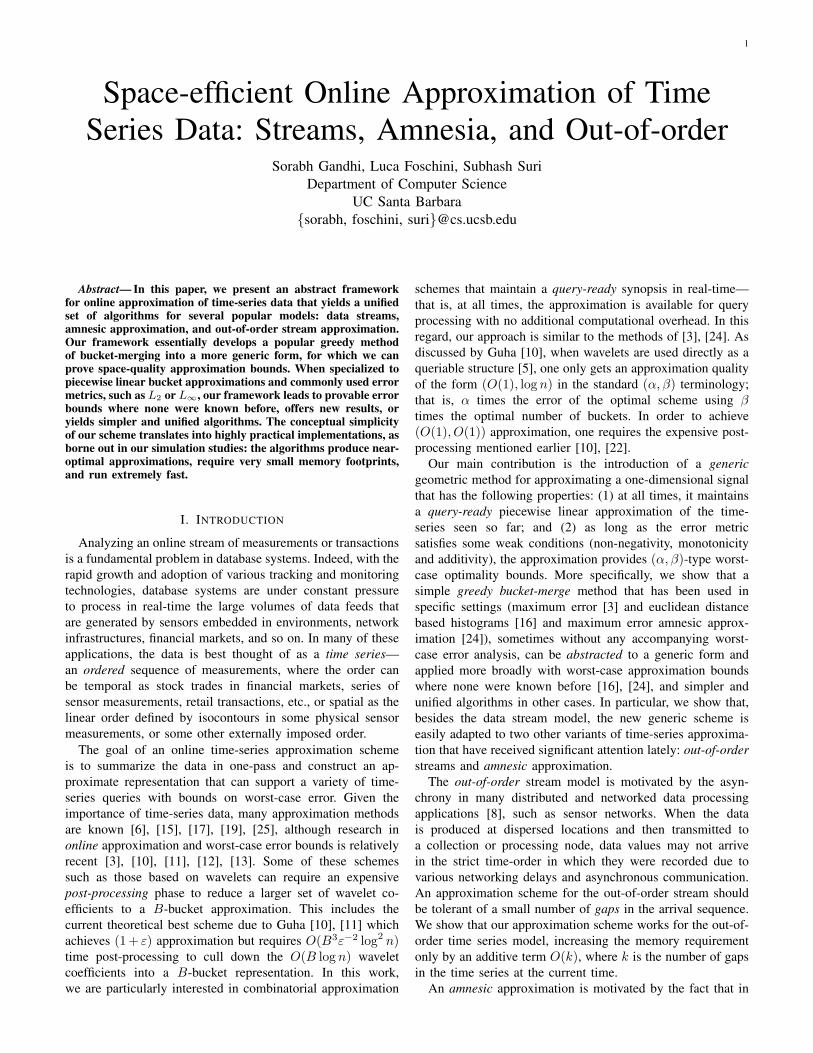
See Figure 3 for an example—the top part shows an examplestream approximated within the error bounds specified by theamnesic error function shown at bottom.

ε1

ε2

ε3

Err

orTol

eran

ce

Age

Original CurveApproximation Buckets

Fig. 3. Amnesic approximation. The top figure shows increasing bucketheights (L∞ error) with increasing data age, and the bottom figure shows amonotone amnesic error function, with 3 age groups.

Next, we describe the amnesic version of our generic mergealgorithm and prove its error bounds. We consider only the L∞norm.

A. Amnesic-Merge (AM) Algorithm

Let the number of age groups in the amnesic function bem, where we assume that m is a small constant and m =o(B). Then, our problem is the following: Given a monotonepiecewise constant amnesic function f(), and a stream S =<v1, v2, . . . , vn > of values, maintain an approximation mini-mizing the number of buckets used such that |vi−vi| ≤ f(xi)for all i, where vi is the approximated value for vi. The mainconceptual difficulty in this amnesic approximation problemarises from the fact that the age of each item changes everytime instant. The simple but key observation in our solutionis the fact that only those buckets that cross the age groupboundaries require special care; the remaining ones behave asin the standard streaming model. This requires only a minorchange to the generic minmerge, and we call this variant theAMNESIC-MERGE (AM) algorithm:

1) Allocate a bucket for the next value in the stream.2) For each age group with two or more buckets in it, if

merging any two adjacent buckets produces error lessthan or equal to the allowable error in the age group,merge the two buckets.

3) Go to Step 1.A bucket is in an age group if its starting timestamp lies

in the age group. This algorithm is nearly identical to thealgorithm proposed in [24] with one minor difference: in thatalgorithm, the merge precedes the allocation of the new bucket,while in our algorithm these steps are reversed.

1) Analysis of the Amnesic-Merge (AM): We first pointout the problem formulation of the amnesic approximation isquite different from our earlier problem. There, we wished tominimize the error given a number B of buckets. In the AMalgorithm, we want to minimize the number of buckets givenerror bounds. We show that if the optimal algorithm uses B∗

optimal buckets for a given amnesic function, then the AMalgorithm uses no more than 3B∗ buckets, while achievingthe same error guarantees for each age group. Thus, AM is a(1, 3) approximation.

Lemma 3: The bucket approximation produced by theAMNESIC-MERGE algorithm satisfies the L∞ error bounds foreach age group, and uses at most 3 times the optimal numberof buckets.

Proof: Let us denote the number of buckets in age groupi by b′i, where age group i is the set of values with age inthe range (τi−1, τi]. As mentioned earlier, the buckets can bethought of as a linear partition of the age axis. There are atmost m−1 buckets which intersect with the partition obtainedby the age groups defined by the amnesic function. Every agegroup i has at least b′i − 1 non-intersecting buckets. Let usdenote the number of non-intersecting buckets associated withage group i by b′′i . Then,

b′′i ≥ b′i − 1 (15)

Assume for now that b′′i ≥ 2. Since we merge buckets onlyif they produce error less than the required error for the agegroup, the buckets in every age group are within the requirederror. Let us denote the set of values in age group i approx-imated by non-intersecting buckets by T ′′i . Let us denote themaximum error in the non-intersecting buckets formed by AMalgorithm in age group i by em(T ′′i , b

′′i ), where b′′i is the

number of buckets used. Also, let us denote the maximumerror in the buckets produced by the optimal algorithm inapproximating set T ′′i using bi buckets by e(T ′′i , bi). Fromthe AM algorithm we know that if there was even one moremerge in the b′′i non-intersecting buckets in age group i, theerror will be more than the allowable error. Hence,

e(T ′′i , b(b′′i − 1)/2)c ≥ em(T ′′i , b′′i − 1) > ei (16)

The first part of this equation follows from the fact that thebuckets obey the Min-Merge property. This equation impliesthat even if one bucket is shared across every neighboring agegroup by the optimal algorithm, with less than (

∑ib(b′i −

1)/2c) − m buckets optimal algorithm cannot achieve thedesired error in every range. Let B = (

∑ib(b′′i − 1)/2c)−m.

We also know that the merge algorithm with at most∑

i(b′i)

buckets achieves the desired error in every range. Let B′ =∑i(b′i). Using this and equation 15 we can show that B′ ≤

2B + O(m) ≤ 3B. (The O(m) terms also takes care of thecase when b′i ≥ 3 does not hold, and since m = o(B), theapproximation still holds.)

To implement the merging of two buckets and computingthe L∞ error of a bucket, we need to maintain the convex hullof the values in each bucket. In the worst case, the size of theconvex hull for a set of n values is O(n), but we can usethe techniques presented in [3] to reduce this size to a userspecified constant. We omit the details and point the reader

7

to [3] for details, and summarize our result in the followingtheorem.

Theorem 5: The AMNESIC-MERGE algorithm achieves a(1 + ε, 3) approximation for the amnesic approximation prob-lem and uses O(ε−1/2B∗ log(1/ε)) space and O(logB∗ +ε−1/2 log(1/ε) update time for each value, where B∗ is thenumber of buckets in the optimal solution.

Remark: Palpanas et al. [24] also propose the dual version ofamnesic approximation problem described above. In the dualversion, we are given an input parameter B, and the constraintson the ratios of the tolerable errors in each age group. It isdifficult to achieve bounds on this problem as the number ofbuckets that needs to be assigned to a contiguous piece of datamight change in a non-monotonic manner depending on theincoming data. We believe that there is a negative result forthis problem and intend to address this issue in a future study.

VI. OUT-OF-ORDER STREAMS

We now discuss an extension of our GENERIC-MINMERGEthat holds for approximating out-of-order streams. The out-of-order stream model is motivated by the asynchrony in manydistributed and networked data processing applications [8],where data is sensed at dispersed locations and then transmit-ted to a central node for processing. Due to various networkingdelays and asynchronous communication, data values may notarrive in the strict time-order in which they were recorded.An approximation scheme for the out-of-order stream shouldbe tolerant of a small number of gaps in the arrival sequence.A gap is maximal block of timestamps [ti, tj ] such that itemswith timestamps ti−1 and tj +1 have arrived but none of theitems with timestamp t, for ti ≤ t ≤ tj , have arrived. We callthe maximal block of timestamps between two consecutivegaps a fragment. Figure 4 shows a snapshot of an out-or-orderstream with gaps and fragments.

GAPS

FRAGMENTS

Fig. 4. Snapshot of an out-of-order stream, showing gaps and fragments.

We are interested in PC or PL bucket approximations usingL2 or L∞ error. A bound on the approximation error meansthat no bucket can include a gap—the missing value can bearbitrarily far off from the approximation. Thus, it is easy tosee that if there are k gaps in the data seen so far, then anguaranteed error approximation requires at least Ω(min(k, n−k)) space. In practice, we assume that the number of gapsis small, and show that our approximation uses space onlylinear in the number of gaps. Our algorithm for the out-of-order streams is called FRAGMENT-MERGE and is describedbelow.

A. The Fragment-Merge (FM) Algorithm

Algorithm 2 gives the pseudocode for the FM algorithm.The value for the constant c is set to 2 for the L∞ norm,and 4 for the L2 norm. At a high level, the algorithm worksas follows. On the arrival of a new value, a new bucket isallocated. Suppose the timestamp associated with the newvalue is ti. Depending on how ti relates to the gaps andfragments, we can have three cases.

1) A new fragment is formed if the values with timestampsti−1 and ti+1 have not been seen so far.

2) The new value is adjacent to exactly one existingfragment—that is, either ti−1 or ti+1 have been seen,but not both.

3) The new value closes the gap between two fragments—that is, both ti−1 and ti+1 have been seen.

These three cases are shown in Figure 5. Depending onwhich category the new value falls in, the FM algorithmperforms 0, 1 or 2 merges. The FRAG-BEST-ADJPAIRfunction returns the two buckets whose merge results in abucket with least error among all adjacent pairs of buckets inall fragments. We analyze this algorithm in the next section.

Algorithm 2 FRAGMENT-MERGE(S, c, B)1: M = ∅, k = 02: for all vi do3: Allocate new bucket u4: M =M

⋃u

5: if |M| ≥ cB + k then6: if Exactly one of the neighboring values of vi has

been seen then7: v1, v2 = FRAG-BEST-ADJPAIR(S)8: v = MERGE(v1, v2)9: M = M \ v1, v2

10: M = M⋃v

11: else if Two neighboring values of vi have been seenthen

12: counter = 013: while counter < 2 do14: v1, v2 = FRAG-BEST-ADJPAIR(S)15: v = MERGE(v1, v2)16: M = M \ v1, v217: M = M

⋃v

18: counter = counter + 119: end while20: k = k − 121: else22: k = k + 123: end if24: end if25: end for

B. Analysis of Fragment-Merge (FM)

We detail the analysis for the L∞ norm, and mention brieflythe case of the L2 norm. Because of the out-of-order arrival ofitems, there are two different notions of time: the timestamp,

8

CASE 1

CASE 3

CASE 2

Incoming Point

Fig. 5. Three different configurations on the arrival of a new item: creationof a new fragment, extension of an existing fragment, and the merging of twoexisting fragments.

which represents the time at which data is generated (at thesource), and the time at which it is received at the processingnode (sink). We use the notation t to denote the source-time and τ to denote the processing or sink-time. Let ki

be the number of fragments at time instant τi. The analysisof FM rests on two lemmas: the first one proves that thebuckets satisfy the Min-Merge property and bounds the sizeof approximation; the second does the error analysis.

Lemma 4: At any time τi, the FRAGMENT-MERGE algo-rithm maintains an approximation of size at most 2B + ki

buckets, where ki is the number of fragments at time τi. Aftereach completed iteration of the algorithm, the buckets obeythe Min-Merge property.

Proof: Our proof is by induction, on the length of thetime series. For the base case, we have one value, so for anyB, we have less than 2B+ki buckets, where ki = 1. We showthat the lemma is true for all iterations of the algorithm afterthe first time instant τj where we have 2B+kj buckets. Beforethe first such time instant the number of buckets is less than2B + ki for any instant τi and the Min-Merge property holdsbecause there have been no merges. We assume that the claimis true for time instant τi and show that the claim is true forτi+1. We separately analyze the three cases mentioned earlier.• Case 1. The new value seen creates a new fragment of

size 1: The number of fragments ki+1 = ki + 1. For thenew value a separate bucket is allocated by the algorithmwhich has zero error. The number of buckets at this pointis 2B + ki + 1, which is 2B + ki+1 and this provesthe first part of the claim. Since the Min-Merge propertywas satisfied at time instant τi, it is also satisfied at timeinstant τi+1 as the new bucket is not merged with anybucket.

• Case 2. The new value increases the length of exactlyone existing fragment by 1: The number of fragmentski+1 = ki. One merge operation is performed, so thenumber of buckets first increases to 2B+ki+1 (allocationof bucket for new value), and then decreases with themerge to 2B+ki, which is the same as 2B+ki+1. Thereare two sub cases that can occur:

– Case a: In the merge operation the new bucket getsmerged with adjacent bucket, say v. Let us say thatthe bucket formed is u. Then, the error of bucket uis no less than the error of bucket v (monotonicityof L∞ error). Hence, the error in the bucket formed

by further merging of u will be no less than theresultant error if v had been merged. But mergingv again would itself result in a bucket with highesterror. This is true as Min-Merge property holds attime τi. Hence the Min-Merge property holds at timeτi+1.

– Case b: In the merge operation, the new bucket isnot merged. Then let us say buckets u′ and v′ getmerged and the error in the resultant bucket is e. Butthis implies that any further merge (including mergeinvolving new bucket), will give a bucket with errorgreater than e, which is the maximum error in theapproximation after (i + 1)th iteration. Hence afterthis one merge Min-Merge property is satisfied.

• Case 3. The new value joins two previously disjointedfragments: This case is similar to Case 2 and its proof isomitted due to lack of space.

This completes the proof.The second lemma establishes the quality of the approxi-

mation formed by FM algorithm with respect to optimal.Lemma 5: At any time τi, the approximation error of the

FRAGMENT-MERGE algorithm using 2B + ki buckets is noworse than the optimal approximation error using B buckets,where ki is the number of fragments at time τi.

Proof: Let us denote the number of buckets used by theoptimal algorithm for fragment j by bj , where 1 ≤ j ≤ ki

and∑ki

j=1 bj = B. Let the error associated with the optimalapproximation using B buckets be E∗. Let us denote the setof values in fragment j by Fj . Let the error associated withoptimal approximation of fragment Fj using bj buckets bee(Fj , bj), and hence E∗ = maxki

j=1 e(Fj , bj).Let us denote the number of buckets used by the FM

algorithm for the jth fragment by b′j , where 1 ≤ j ≤ ki and∑ki

j=1 b′j ≤ 2B + ki. Let the corresponding error associated

with fragment j be em(Fj , b′j). The overall error of the

approximation is E = maxkij=1 em(Fj , b

′j). We want to show

that E ≤ E∗. We will show the result by contradiction, andhence let us assume the following,

E∗ < E (17)

For the above equation to be true, there must exist at leastone u, such that b′u < 2bu. This follows from the fact thatevery fragment follows the Min-Merge property (Theorem 3).Without loss of generality, let this be the fragment whichresults in the maximum error i.e.

E = em(Fu, b′u) (18)

Then, there must also be at least one fragment v, suchb′v > 2bv + 1 (Pigeon hole principle). Now, consider the lastalgorithm iteration which resulted in the number of buckets foru to go from b′u + 1 to b′u. Note that there could be multiplesuch merges and we consider the last such merge before timeinstant τi, say at time instant τj . At time instant τj , fragmentv has either more than 2bv buckets, or less (equal to) than2bv buckets. We handle the arguments for these two casesseparately.

9

• Case 1: If v has more than 2bv buckets, say it has b′′vbuckets, and let the fragment itself at that time be F ′vwhere F ′v ⊆ Fv , then

em(F ′v, b′′v − 1) ≤ e(Fv, bv) ≤ E∗ (19)

This follows from the fact that the fragments obey Min-Merge property and the buckets obeying Min-Merge givesa (1, 2) approximation for L∞ error (Theorem 3). But,FM algorithm merges u before v, so error in fragment vafter one merge, is no less than the error in fragment uwhen it has b′u buckets,

em(F ′v, b′′v − 1) ≥ em(Fu, b

′u) (20)

Combining equations 18, 19 and 20, we get E∗ ≥ E,which contradicts our assumption.

• Case 2: At time instant τj , fragment v has less than (orequal to) 2bv buckets. Then there must be a new valueat some other time instant, say τl, where τl is after τjwhich results in v having more than 2bv + 1 buckets(after completed iteration of FM merge). This value canbe either one which is next to one end of a fragment (asin Case 2, Lemma 4) or it can be the value which joinstwo fragments (as in Case 3, Lemma 4). We leave outthese cases in the interest of space.

This concludes the proof.With the natural assumption that ki ≤ B, we get that

2B+ki ≤ 3B. The analysis above requires us to maintain theconvex hull of the values in each bucket in order to determinethe approximation error in the bucket. Using the approximateconvex hulls as in [3], we can get an ε approximation. Dueto space constraints, we skip those details, and state the mainresult for this section.

Theorem 6: The FRAGMENT-MERGE algorithm achieves a(1 + ε, 3) approximation for the piecewise linear approxima-tion of an out-of-order stream under the L∞ norm, usingO(ε−1/2B log(1/ε)) space and O(logB + ε−1/2 log(1/ε))update time for each value.

For piecewise constant approximation, the space and timebounds are O(B) and O(logB) respectively, for a (1, 3)approximation for the L∞ norm. We can show a similar resultfor the L2 approximation.

Theorem 7: The FRAGMENT-MERGE algorithm gives a(√

2, 5) approximation for the piecewise constant (or piece-wise linear) approximation of an out-of-order stream underthe L2 norm using O(B) space and O(logB) update time foreach value.

VII. SIMULATION RESULTS

In this section, we report on the simulation-based perfor-mance evaluation of our three main algorithms, for computinghistogram for streams (L2 approximation), histograms foramnesic approximation (L∞ approximation), and the out-of-order stream approximation. In particular, we implementedthe following algorithms, including some optimal schemes forbenchmarking. (All the code is written in Python or C++, andis available at www.cs.ucsb.edu/˜foschini/files/ooodelay.zip,along with the instructions to run it. All the benchmarks

reported in this paper are run on an Intel Core Duo Processor(@ 2.00GHz) equipped with 2GB RAM.)

• GENERIC-MINMERGE, AMNESIC-MERGE, FRAGMENT-MERGE: We implemented all three main variants of ourgeneric scheme (GM, AM and FM).

• Dynamic Programming: We implemented the dynamicprogramming scheme described in [14] for computingthe optimal error histogram approximation. We onlyuse the optimal histogram for error comparison, and sotechniques for improving the space bounds are irrelevantin this case [10].

• SPACEAPXWAVEHIST Algorithm: We also implementedGuha’s algorithm described in [10], which currently hasthe best theoretical approximation bound1. (More detailsabout this can be found in Section VII-A.3. For perfor-mance reasons, this algorithm is implemented in C++.)

• Optimal Amnesic Approximation: We implemented theoptimal (offline) amnesic approximation scheme. Thisalgorithm processes values in order of decreasing (source)timestamps. Initially the algorithm starts with an emptybucket. Values are added to the bucket as long as theerror in the bucket is less than the tolerable error forthe highest timestamp value in the bucket. If not, a newbucket is started, and so on.

In our experiments, we used a variety of datasets fromvarious applications. From these, 5 datasets are shown inFigure 6.

• STEAMGEN [18]: The set has 9600 measurements of thedrum pressure, taken every 3 seconds, from a model ofa steam generator at Abbott Power Plant in ChampaignIL.

• RANDOM [18]: This is the classical random walk dataused in many papers on time series indexing. This setconsists of 65536 values.

• DJIA: This set has the value of the Dow Jones IndustrialAverage index starting from year 1900. We obtained thisdataset from StatLib and it consists of 25737 values.

• HUM: This set consists of measurements from humiditysensors monitoring servers in a large data center. It has69652 values, representing humidity measurements every30 seconds.

• TEMP: This set of 93861 values consists of temperaturereadings taken once every 5 minutes from the Davisweather station in Amherst, Massachusetts.

We begin by evaluating the quality of approximations pro-duced by the GM algorithm and demonstrating the scalabilityof the scheme in Section VII-A. In Section VII-B we comparethe performance of AM algorithm with the optimal offlinealgorithm. And finally, in Section VII-C we demonstrate thequality of approximations produced by the FM algorithm forout of order streams.

1[11] provides similar bounds as [10], the postprocessing time is nearlythe same for both the algorithms and this is what we compare with GM andhence we implement only SpaceApxWaveHist.

10

150

200

250

300

350

400

450

500

550

0 500 1000 1500 2000 2500 3000 3500 4000-40

-30

-20

-10

0

10

20

30

40

50

60

0 500 1000 1500 2000 2500 3000 3500 4000 40

50

60

70

80

90

100

110

0 500 1000 1500 2000 2500 3000 3500 4000 24

26

28

30

32

34

36

38

40

42

0 500 1000 1500 2000 2500 3000 3500 4000 10

15

20

25

30

35

40

45

50

55

60

0 500 1000 1500 2000 2500 3000 3500 4000

Fig. 6. Left to Right: STEAMGEN, RANDOM, DJIA, HUM and TEMP

A. Minmerge for the L2 Histograms

We evaluate the quality and scalability of L2 histogramapproximation by our generic minmerge algorithm GM. (Aminmerge type algorithm for the L∞ histogram was alreadypresented in [3].) Curiously, algorithms that use greedy bucket-merges for the L2 streaming histograms have been used widelybefore, but with no worst-case error bounds [16], [24]. In fact,there is only one minor difference in the details of our GM andthe GRAP-R algorithm [16]: we do the merge after allocatingthe new bucket for the new item, while GRAP-R does themerge first. Empirically, this minor change has little effect onthe performance of the algorithm, but it does allow us to provea worst-case error bound for GM.

1) The Approximation Quality: We compare the quality ofthe approximations produced by the GM algorithm with thedynamic programming scheme. Because dynamic program-ming has quadratic time complexity, it is extremely slowfor large data sets, so we ran our test using n = 4000values. The results are shown in Figure 7, which plots theL2 approximation error vs. the number of buckets.

Our results were virtually identical across all 5 data sets, sothis figure shows a representative sample for the HUM data set.In the experiment, we vary the buckets from 50 to 200. (Sincethe slowness of the dynamic programming limited us to 4Ksize data sets, there did not seem to be a point in increasingthe number of buckets to larger values. In later experimentson larger data sets, we allow larger values of B.)

The total error predictably decreases with an increasingnumber of buckets. Recall that Theorem 4 gives a (

√2, 4)

approximation guarantee, meaning that the error of the GMhistogram using 4B buckets is no worse than

√2 times the

error of the optimal B-bucket histogram. Thus, Figure 7 shows3 bars for each value of B: the leftmost bar is the optimal error;the middle bar is the error of the GM using 4B buckets; andthe rightmost bar is the error of the GM using just B buckets.The left part shows the results for PC histograms and the rightpart shows the results for PL histograms. These results showthat GM’s performance is much better than the worst-caseguarantee: with 4B buckets, the error is about a third of theoptimal error, and even with the same memory as optimal (Bbuckets), the error of the GM approximation is only slightlyworse (never more than 30%).

In fact, for the rest of the empirical evaluations, even forAM and FM algorithms, we always use only B buckets forour algorithms, and not the constant-factor-times B bucketsrequired by our theorems.

2) Scalability of GM algorithm: In this experiment weevaluate the scalability (processing time) of the GM algorithmas a function of the size of the stream. We use a large dataset

50 75 100 125 150 175 200# of Buckets (B)

0

5

10

15

20

25

L2 E

rror

OPT

4B-GM

B-GM

50 75 100 125 150 175 200# of Buckets (B)

0

5

10

15

20

25

L2 E

rror

OPT

4B-GM

B-GM

Fig. 7. The approximation quality as a function of the number of buckets,for the HUM data. The results shown are for PC histograms (left) and PLhistograms (right). B-GM refers to the B-bucket approximation, while 4B-GM refers to the 4B-bucket approximation (as needed for the theorem).

200K 400K 600K 800K 1000KStream Size (n)

0

1e-4

2e-4

Tim

e p

er

poin

t (s

)

1000

5000

9000

Fig. 8. Per-item processing time vs. the size of the time stream, for B =1000, 5000, 9000 for the PRECIP dataset.

to show the scalability, we call this dataset PRECIP. Thearchive [27] contains the average monthly and annual gage-corrected precipitation recorded by 26, 858 stations worldwide.Station averages of precipitation are interpolated to a 0.5degree by 0.5 degree of latitude/longitude grid, where thegrid nodes are centered on 0.25 degree, resulting in 259200geographically distinct measurements. The dataset PRECIPhere analyzed contains 1M values from the previous archiveobtained by concatenating the measurements for all stationsfor several months after having sorted the archive on (latitude,longitude) of the stations.

We vary the size of the dataset from 200K to 1M inintervals of 200K and plot the time taken per data pointby the GM algorithm for different number of buckets: B =1000, 5000, 9000. The results are shown in Figure 8 for PCapproximation. As predicted by theory, the GM algorithmscales linearly with the size of the stream and shows anegligible effect of the number of buckets. The results for PLapproximations are the same, just that it takes more processingtime per data point (roughly a factor of 3 more).

3) Comparison with SPACEAPXWAVEHIST: The currentbest theoretical bound for the L2 histogram approximationis due to Guha [10]: his SPACEAPXWAVEHIST algorithmachieves (1+ε, 1) approximation in O(n+B3ε−2 log2 n) timeusing O(Bε−2 log n log ε−1) space. Our GM algorithm only

11

guarantees a (√

2, 4) approximation, but has the advantageof utter simplicity, as well as generalizability to models suchas amnesic and out-of-order streams. A second, and perhaps,more significant advantage of our scheme may be that it main-tains a query-ready indexable structure at all times. In otherwords, our time series approximation is directly representedas a histogram that can be queried at any time, with noadditional overhead. This is in contrast to schemes such asGuha’s [10] whose synopses consist of wavelet coefficientsthat must be processed to build a B bucket histogram. Theoverhead of this post-processing requirement for the guar-antee can be significant—for instance, the technique in [10]requires O(B3 log2 n) time to build the B bucket histogrambefore a query can be answered. Thus, the two schemes,ours and Guha’s, have different advantages—the latter hasthe best provable worst-case error guarantee while the formermaintains an online query-ready histogram—so it is worthcomparing the two in a simulation.

Since a public implementation of SPACEAPXWAVEHISTwas no available, we implemented it ourselves. After someoptimizations and parameter tuning, the observed performanceseems to match with what is reported in [10], so we feel thatour comparisons should be fair. Figures 9 shows the mainresults of our experiments (for HUM dataset): the error in theapproximation of the GM algorithm (using the same amount ofmemory) is close to that achieved by SPACEAPXWAVEHIST(the left figure), however the running time of that algorithm issignificantly worse than GM (as predicted by theory), as shownin the right figure. Results for other datasets are virtually thesame. The SPACEAPXWAVEHIST scheme uses memory in twoplaces, wavelet synopsis and partial dynamic programmingtable. Rather than optimize the memory distribution acrossthese two components, we allocated to each part as muchmemory as our GM scheme requires, thereby potentially givingSPACEAPXWAVEHIST twice the memory. More details of theexperiment are omitted due to lack of space.

100 150 200 250 300 350 400 450 500# of buckets (B)

50

100

150

200

250

300

L2 e

rror

B-GM

SpaceApxWaveHist

100 150 200 250 300 350 400 450 500# of buckets (B)

50

0

50

100

150

200

250

300

350

Tim

e (

s)

B-GM

SpaceApxWaveHist

Fig. 9. GM vs. SPACEAPXWAVEHIST. The approximation error (left) of B-bucket GM is comparable to the B-bucket SPACEAPXWAVEHIST, with thelatter given twice the working space. The running time of GM is significantlyfaster, due to the O(B3) term in SPACEAPXWAVEHIST.

B. The Amnesic Time Series Approximation

In order to set up a natural aging function, we dividedthe data into 4 groups, with approximation error set to 1%,2%, 3% and 4%, respectively, of the maximum data range,where the data range is defined as the difference between themaximum and the minimum value. The spread of the groups isexponential. In other words oldest n/2 are allowed error 4%,

1.0 1.2 1.4 1.6 1.8 2.0 2.2 2.4 2.6Scale

50

100

150

200

250

300

# o

f B

uck

ets

(B

)

B-AM

OPT

Fig. 10. The number of buckets required by the AM (B-AM) algorithm ascompared to optimal for different scaling factors for the DJIA dataset.

the next n/4 values are allowed error 3% and so on. Thus,we have a monotone piecewise constant amnesic function with4 steps. We also used a scaling function to adjust the valuesof the allowable errors, while keeping their ratio the same.In other words, by using a scaling factor of 2, we get theapproximation errors for the 4 age groups to be 2.0%, 4.0%,6.0% and 8.0%.

The approximation quality for the amnesic histogram isgiven by the number of buckets used by the AM algorithm,so we compare this to the optimal amnesic approximation.We show the results of the streaming amnesic approximationfor one representative data set (DJIA), which contains 25Kdata points. Our results for PC approximations are shown inFigure 10. One can see that the number of buckets used bythe AM algorithm closely track the optimal number of bucketsand typically within a factor 1.2 of the optimal number ofbuckets. The results for the other datasets for both PC and PLapproximations are similar; the factors go up to 1.3.

C. Performance of the Fragment-Merge (FM)

40 60 80 100 120 140 160 180 200# of Buckets (B)

600

700

800

900

1000

1100

1200

1300

1400

1500

L2 E

rror

Bursty

Ordered

Perturbation

40 60 80 100 120 140 160 180 200# of Buckets (B)

10

15

20

25

30

35

40

L∞

Err

or

Bursty

Ordered

Perturbation

Fig. 11. The quality of approximation produced for the Bursty, Perturbationand the Ordered stream models for L2 (left) and L∞ (right) error metrics.The FM algorithm adapts very well for out of order arrivals.

Our last set of experiments analyze the performance of theFRAGMENT-MERGE algorithm for approximating out-of-orderstreams. We first describe our data model for generating arealistic out-of-order stream. There are two aspects to this:how frequently an item appears out of order, and how farfrom its true position it reappears. Let us first consider thesecond question. Using the Internet as a guide, we envisiontwo different models for packet delay: a bursty model, whichmay account for buffer overflow at a node causing many datavalues to be lost and retransmitted, and a perturbation model,which may account for the multi-path routing phenomenon innetworking, causing packets to arrive slightly out of order. For

12

the first question, we use a correlated random model to decidewhich data value to delay.

In more details, we construct an out-of-order stream froman ordered stream statistically in the following manner. Theith item in the stream is reordered (delayed) with probabilitypi, given as follows:

pi =(1− χ) · ρ+ χ · Ii−1

Ii−1 + ρ, (21)

where ρ is the independent probability for an item to bereordered, χ is the correlation probability that accounts forthe previous item being reordered, and Ii−1 is the indicatorvariable which is either 1 or 0 depending on whether the(i−1)th value was reordered or not. In order to simulate this,for the ith value we flip a coin biased with probability pi. Oncean item is taken out, it is reinserted later in the stream with adelay uniformly distributed between 0 and L (lag). Thus, ourreordering strategy is completely described by the parametersχ, ρ and L. The bursty model is simulated with small valueof ρ, and large values for χ and L. The perturbation model issimulated with large value of ρ, and small values of χ and L.(Due to space constraints, we omit the details.)

We evaluate the error performance of the FM algorithmby comparing it with the approximation obtained by the GMalgorithm for the ordered version of the stream. Figure 11shows the results of this experiment for the DJIA data, wherethe out-of-order streams are generated both with the burstyand the perturbation models, and the plot shows the error ofthe approximation vs. the bucket parameter B.

The figure on the left shows the L2 approximation, whilethe one on the right shows the L∞ approximation. In bothcases, it is easy to see that the error of the FRAGMENT-MERGE approximation is very close to the error of the GMapproximation for the ordered version of the stream. In somecases, the FM error approximation is actually smaller thanthe GM approximation, but that is explained by the fact theFM approximation uses a maximum of B + k buckets, wherek is the number of gaps in the stream, while the orderedstream uses only B buckets. In this set of experiments, themaximum number of gaps for the bursty model is 84, and forthe perturbation model it is 23.

We also ran scalability for experiments for both AM andFM algorithms. The results for these are very similar to theGM algorithm, though individual per item processing timesare slightly slower for both AM and FM as compared to GM.

VIII. CONCLUSIONS AND FUTURE WORK

We presented a generic framework for online approxima-tion of time-series data that yields a unified set of algo-rithms for several popular models: data streams, amnesicapproximation, and out-of-order stream approximation. Ourframework essentially develops a popular greedy method ofbucket-merging into a more generic form, for which we canprove space-quality approximation bounds. When specializedto piecewise linear bucket approximations and commonly usederror metrics, such as L2 or L∞, our framework leads toprovable error bounds where none were known before, offers

new results, or yields simpler and unified algorithms. Theconceptual simplicity of our scheme translates into highlypractical implementations, as borne out in our simulationstudies: the algorithms produce near-optimal approximations,require very small memory footprints, and run extremely fast.

Acknowledgments: We thank Sudipto Guha for helping usunderstand the details of his algorithm during our implemen-tation, Eamonn Keogh for giving us access to time series data,and Themis Palpanas for clarifying one of the proofs in [24].

REFERENCES

[1] M. Abam, M. Berg, P. Hachenberger, and A. Zarei. Streaming algorithmsfor line simplification. In SOCG, 2007.

[2] B. Babcock, S. Babu, M. Datar, R. Motwani, and J. Widom. Modelsand issues in data stream systems. In PODS, 2002.

[3] C. Buragohain, N. Shrivastava, and S. Suri. Space efficient streamingalgorithms for the maximum error histogram. In ICDE, 2007.

[4] C. Busch and S. Tirthapura. A deterministic algorithm for summarizingasynchronous streams over a sliding window. In STACS, 2007.

[5] K. Chakrabarti, M. Garofalakis, R. Rastogi, and K. Shim. Approximatequery processing using wavelets. The VLDB Journal, 10(2-3), 2001.

[6] K. Chan and A. Fu. Efficient time series matching by wavelets. InICDE, 1999.

[7] Y. Chen, G. Dong, J. Han, B. Wah, and J. Wang. Multidimensionalregression analysis of time-series data streams. In ICDE, 2002.

[8] G. Cormode, F. Korn, and S. Tirthapura. Time-decaying aggregates inout-of-order streams. In PODS, 2008.

[9] A. Gilbert, Y. Kotidis, S. Guha, S. Muthukrishnan, et al. Fast small-spacealgorithms for approximate histogram maintenance. In STOC, 2002.

[10] S. Guha. On the space—time of optimal, approximate and streamingalgorithms for synopsis construction problems. The VLDB Journal,17(6):1509–1535, 2008.

[11] S. Guha. Tight results for clustering and summarizing data streams.In Departmental Papers, Department of Computer and InformationScience, Univeristy of Pennsylvania, 2009.

[12] S. Guha, N. Koudas, and K. Shim. Data-streams and histograms. InSTOC, 2001.

[13] S. Guha, N. Koudas, and K. Shim. Approximation and streaming al-gorithms for histogram construction problems. ACM TODS, 31(1):396–438, 2006.

[14] H. Jagadish, N. Koudas, S. Muthukrishnan, V. Poosala, et al. Optimalhistograms with quality guarantees. In VLDB, 1998.

[15] E. Keogh, K. Chakrabarti, S. Mehrotra, and M. Pazzani. Locally adaptivedimensionality reduction for indexing large time series databases. InSIGMOD, 2001.

[16] E. Keogh, S. Chu, D. Hart, and M. Pazzani. An online algorithm forsegmenting time series. In In ICDM, 2001.

[17] E. Keogh and M. Pazzani. A simple dimensionality reduction techniquefor fast similarity search in large time series databases. In PADKK,2000.

[18] E. Keogh, X. Xi, L. Wei, and C. Ratanamahatana. The ucr time seriesclassification/clustering homepage. 2006.

[19] F. Korn, H. Jagadish, and C. Faloutsos. Efficiently supporting ad hocqueries in large datasets of time sequences. In SIGMOD, 1997.

[20] J. Li, K. Tufte, V. Shkapenyuk, V. Papadimos, T. Johnson, and D. Maier.Out-of-order processing: a new architecture for high-performance streamsystems. Proc. VLDB Endow., 1(1), 2008.

[21] M. Li, M. Liu, L. Ding, E. Rundensteiner, and M. Mani. Event streamprocessing with out-of-order data arrival. In ICDCS Workshop, 2007.

[22] S. Muthukrishnan and S. Strauss. Approximate histogram and waveletsummaries of streaming data. In DIMACS TR 52, 2003.

[23] S. Nath. Energy efficient sensor data logging with amnesic flash storage.In IPSN, 2009.

[24] T. Palpanas, M. Vlachos, E. Keogh, D. Gunopulos, and W. Truppel.Online amnesic approximation of streaming time series. In ICDE, 2004.

[25] D. Rafiei and A. Mendelzon. Similarity-based queries for time seriesdata. In SIGMOD, 1997.

[26] P. Tucker, D. Maier, T. Sheard, and L. Fegaras. Exploiting punctuationsemantics in continuous data streams. IEEE Trans. on Knowl. and DataEng., 15(3), 2003.

[27] C. Willmott and K. Matsuura. Global air temperature andprecipitation: Regridded monthly and annual climatologies. Inhttp://climate.geog.udel.edu/.