sovereign default swap market efficiency and country risk ...... discussion paper deutsche...
TRANSCRIPT

Discussion PaperDeutsche BundesbankNo 08/2013
Sovereign default swap market efficiency and country risk in the eurozone
Yalin Gündüz(Deutsche Bundesbank)
Orcun Kaya(Goethe University Frankfurt)
Discussion Papers represent the authors‘ personal opinions and do notnecessarily reflect the views of the Deutsche Bundesbank or its staff.

Editorial Board: Klaus Düllmann
Heinz Herrmann
Christoph Memmel
Deutsche Bundesbank, Wilhelm-Epstein-Straße 14, 60431 Frankfurt am Main,
Postfach 10 06 02, 60006 Frankfurt am Main
Tel +49 69 9566-0
Please address all orders in writing to: Deutsche Bundesbank,
Press and Public Relations Division, at the above address or via fax +49 69 9566-3077
Internet http://www.bundesbank.de
Reproduction permitted only if source is stated.
ISBN 978–3–86558–8
ISBN 978–3–86558–8
94–4 (Internetversion)
93–7 (Printversion)

Non-technical summary
Credit default swaps (CDSs) are financial derivatives that are designed to transfer credit
risk between banks, hedge funds or asset managers in a simple way: The buyer of the CDS
is insured by the seller against the default of the underlying sovereign entity. The insurance
premium (or “the CDS spread”) of these CDSs written on sovereign entities have been
seen as an important indicator of the economic health of a given country. This paper uses
CDS spread changes as a measure for the informational efficiency of the sovereign markets
and CDS spread volatilities as a proxy for persistency of country risks. Specifically, we
test whether the dependence of consecutive observations dies out slowly over time (“long
memory”). We firstly show that there is no evidence of such behavior of CDS spread
changes for any of the 10 eurozone countries in our sample. This indicates that, despite
the financial crisis and uncertainty of financial markets, price discovery processes satisfy
the minimum requirements for a weak form of market efficiency for sovereign CDSs, i.e.
recent CDS spread changes cannot be predicted with past CDS spread changes. Second,
there is strong evidence of long memory for volatility patterns of spread changes for 6
out of 10 countries. Specifically, we observe Greece, Portugal, Ireland, Italy, Spain, and
Belgium to demonstrate such behavior. This shows that economies in the eurozone, which
have been particularly affected by the financial and the sovereign debt crisis, are exposed
to high uncertainty risk not only for a short period but over a persistent horizon. Third,
we illustrate that CDS volatility is causal to CDS levels, indicating that uncertainty in
CDS markets translates into higher risk premia for sovereign risk. Finally, we highlight
the existence of a comovement of CDS spread changes for all countries, which is more
explicit among peripheral economies. Our results have implications on selecting sovereign
risk measures: Increased global risk aversion and the uncertainty about future sovereign
debt market conditions have caused an increase in sovereign CDS volatility, which has
been shown to be a meaningful measure of sovereign risk.

Nicht-technische Zusammenfassung
Credit Default Swaps (CDS) sind Finanzderivate, die eine einfache Ubertragung von
Kreditrisiken zwischen Banken, Hedgefonds oder Vermogensverwaltern ermoglichen: Der
Kaufer des CDS wird vom Verkaufer gegen den Ausfall des zugrunde liegenden staatlichen
Schuldners abgesichert. Die Versicherungspramie (oder CDS-Pramie) von CDS auf Staat-
sanleihen gilt als wichtiger Indikator fur die wirtschaftliche Lage eines Landes. Die
vorliegende Arbeit untersucht anhand der Veranderungen von CDS-Pramien die Infor-
mationseffizienz der CDS-Markte und anhand ihrer Volatilitat die Persistenz von Lander-
risiken. Insbesondere wird getestet, inwiefern die fortlaufenden Beobachtungen uber die
Zeit voneinander abhangig sind (“Langzeitgedachtnis”). Dabei wird gezeigt, dass sich im
Hinblick auf die Entwicklung der CDS-Pramien in den zehn untersuchten Euro-Landern
keine Belege fur ein “Langzeitgedachtnis” finden lassen. Dies deutet darauf hin, dass
aktuelle Veranderungen von CDS-Pramien nicht mit Hilfe fruherer Veranderungen von
CDS-Pramien prognostiziert werden konnen. Folglich erfullen die Preisbildungsprozesse
an den Markten fur CDS auf Staatsanleihen trotz der Finanzkrise und der Unsicherheit
an den Finanzmarkten die Mindestanforderungen fur eine schwache Form von Marktef-
fizienz. Andererseits gibt es bei sechs der zehn in der Stichprobe untersuchten Lander
eine starke Evidenz fur ein “Langzeitgedachtnis” im Hinblick auf die Volatilitatsmuster
der Pramienentwicklung. Ein solches Verhalten ist speziell in Griechenland, Portugal,
Irland, Italien, Spanien und Belgien zu beobachten; dies belegt, dass Lander des Euro-
Wahrungsgebiets, die von der Finanz- und Staatsschuldenkrise besonders betroffen waren,
nicht nur kurzfristig, sondern uber einen langeren Zeithorizont hinweg dem Risiko hoher
Unsicherheit ausgesetzt sind. Des Weiteren wird aufgezeigt, dass sich die Volatilitat
von CDS-Pramien kausal zum CDS-Niveau verhalt, sodass sich Unsicherheit an den
CDS-Markten in hoheren Risikopramien fur Landerrisiken niederschlagt. Abschließend
wird aufgezeigt, dass die Veranderung der CDS-Pramien in allen untersuchten Landern
einen Gleichlauf aufweist, der bei den Peripherielandern deutlicher zutage tritt. Unsere
Ergebnisse haben Implikationen fur die Wahl geeigneter Messgroßen des Landerrisikos:
Die gestiegene globale Risikoaversion und die Unsicherheit im Hinblick auf die kunftige
Entwicklung an den Staatsanleihemarkten haben einen Anstieg der an den Markten
fur CDS auf Staatsanleihen beobachteten Volatilitat bewirkt, die erwiesenermaßen eine
aussagefahige Messgroße des Landerrisikos darstellt.

Sovereign Default Swap Market Efficiency and
Country Risk in the Eurozone∗
Yalin Gunduz† Orcun Kaya‡
Abstract
This paper uses sovereign CDS spread changes and their volatilities as a proxy for
the informational efficiency of the sovereign markets and persistency of country risks.
Specifically, we apply semi-parametric and parametric methods to the sovereign
CDSs of 10 eurozone countries to test the evidence of long memory behavior during
the financial crisis. Our analysis reveals that there is no evidence of long memory
for the spread changes, which indicates that the price discovery process functions
efficiently for sovereign CDS markets even during the crisis. In contrast, both
semi-parametric methods and the dual-parametric model imply persistent behavior
in the volatility of changes for Greece, Portugal, Ireland, Italy, Spain, and Belgium
addressing persistent sovereign uncertainty. We provide evidence of causality from
volatility in CDS prices to sovereign risk premiums for these peripheral economies.
We furthermore demonstrate the potential spillover effects of spread changes among
eurozone countries by estimating dynamic conditional correlations.
Keywords: Credit default swaps, long memory, sovereign risk, eurozone economies,
FIGARCH, dynamic conditional correlation.
JEL-Classification: C22, C58, G01, G15
∗The authors thank Jorg Breitung, Virginie Coudert, Klaus Dullmann, Robert Engle, MichaelHaliassos, Jan Scheithauer, Marliese Uhrig-Homburg, participants of the 5th Financial Risks InternationalForum on Systemic Risk, 2012 Paris; Society for Nonlinear Dynamics and Econometrics 20th Symposium,2012 Istanbul; Financial Management Association European Conference, 2012 Istanbul; InternationalFinance and Banking Society Conference, 2012, Valencia; European Financial Management AssociationConference, 2012 Barcelona; Econometric Society European Meetings, 2012 Malaga; CREDIT: 11thInternational Conference on Credit Risk Evaluation, 2012 Venice; seminar participants at GoetheUniversity Frankfurt and Deutsche Bundesbank for helpful comments and suggestions. We gratefullyacknowledge the programme committee of Society for Nonlinear Dynamics and Econometrics 20thSymposium for being selected for the Gerald P. Dwyer Best Paper in Finance Award. The views expressedherein are our own and do not necessarily reflect those of Bundesbank.†Yalin Gunduz is a Financial Economist at the Deutsche Bundesbank, Wilhelm Epstein Str.
14, 60431 Frankfurt, Germany. Phone: +49 (69) 9566-8163, Fax: +49 (69) 9566-4275, E-mail:[email protected].‡Orcun Kaya (Contact author) is associated with the Goethe University Frankfurt, Department of
Money and Macroeconomics, House of Finance, Gruneburgplatz 1, 60323, Frankfurt, Germany. Phone:+49 (69) 798 33827, E-mail: [email protected]
BUNDESBANK DISCUSSION PAPER NO 08/2013
Sovereign Default Swap Market Efficiency and
Country Risk in the Eurozone
1 Introduction
Credit default swaps (CDSs) of sovereign debt have been the subject of enormous attention
and criticism since the beginning of the credit crunch in mid 2007. Similar to other
credit derivatives, sovereign CDSs are financial derivatives that are designed to transfer
credit risk between banks, hedge funds or asset managers in a simple way: The buyer of
the CDS is insured by the seller against the default of the underlying sovereign entity.
Moreover, CDSs written on sovereign entities have been seen as an important indicator of
the economic health of a given country. They shed light on the default risk by signaling
how much investors are willing to pay to insure themselves against the sovereign risk.
It is now a known fact that many eurozone countries suffer from severe public deficit
problems which they are trying to finance through sovereign indebtedness. For instance,
Greece, being one of the most indebted countries in Europe, has a public debt level
equivalent to 113% of that country’s GDP. Other European countries such as Portugal,
Italy, Ireland, Belgium and Spain face similar public debt problems. Given that sovereign
CDSs serve as a market indicator of the riskiness of public debt, the spread changes
and volatility patterns are strongly linked to the efficient pricing of public debt and to
the fluctuations in the perception of country risk (Longstaff et al. (2011), Grossman and
Huyck (1988)).
This paper investigates the long memory properties of sovereign CDSs for 10 eurozone
countries. CDS spread changes and volatilities have been analyzed as a proxy for the
informational efficiency of the sovereign markets and the persistence of uncertainty. All
other things being equal, the long-memory behavior of sovereign CDS spread changes
would imply strong predictability and an untrustworthy price discovery process where
the most up-to-date information about the market perception of the sovereign CDSs is
not priced correctly. This indeed could create arbitrage possibilities for the issuers of
1

these products. On the other hand, as a proxy for investment risk, the long memory of
volatility patterns sheds light on the overall health of the economy and can be used to
predict future economic variables such as GDP.1
We also analyze the possibility that the CDS spread changes could be correlated among
the 10 eurozone countries. A higher correlation among sovereign CDS markets of the
eurozone economies would imply a more integrated structure. The evolution of the
comovement of sovereign CDS markets as well as the magnitude of the correlations shed
light on the spillover effects, which are especially important during crisis periods.
Our analysis follows a three-step process. We first test for long memory behavior for
both CDS spread changes and squared changes employing different tests and robust-
ness parameters. Specifically, we employ the log periodogram regression of Geweke and
Porter-Hudak (1983) and the modified log periodogram regression of Phillips (2007) for
different ordinate lengths. Second, we model the long memory of spread change and
squared spread change series using a dual long memory model. The dual memory method,
which is a combination of Granger and Joyeux (1980) ARFIMA and Baillie et al. (1996)
FIGARCH models, allows us to estimate the long memory parameters of spread changes
while simultaneously estimating their volatility. Third, we focus on the spillover effects
by employing the dynamic conditional correlation model of Engle (2002) and by utilizing
a two-stage estimation methodology.
Our main results can be summarized as follows: First, we have shown that there is
no evidence of long memory behavior of CDS spread changes for any of the countries in
our sample. This indicates that, despite the financial crisis and uncertainty of financial
markets, price discovery processes satisfy the minimum requirements for a weak form of
market efficiency for sovereign CDSs. On the other hand, there is strong evidence of long
memory for volatility patterns of spread changes for 6 out of 10 countries. Specifically,
we observe Greece, Portugal, Ireland, Italy, Spain, and Belgium to demonstrate such
behavior, which shows that the troubled economies in the eurozone which experience
1i.e. Campbell et al. (2001) show that stock market volatility helps to predict GDP growth.
2

serious instability are exposed to high uncertainty risk not only for a short period but
over a persistent horizon. Third, we illustrate that CDS volatility is Granger-causal to
CDS levels, indicating that uncertainty in CDS markets translates into higher sovereign
risk levels. Finally, we highlight the existence of a comovement of CDS spread changes
for all countries, which is more explicit among less stable economies.
Our paper contributes to several strands of the literature. First and foremost, it extends
the econometric literature on the time series properties of CDS markets. Specifically, we
provide evidence of long memory properties for the volatility of sovereign CDS spread
changes. Even though CDS prices appear to have increased tremendously after the
crisis, we have shown that price discovery and information mechanisms still seem to be
functioning properly. In the light of our results, we can argue that speculative actions
using sovereign CDSs through hedge funds or banks are less likely. Previous literature
provides evidence of volatility transmissions among CDSs, equity, and bond markets
(Belke and Gokus (2011)). If the sovereign CDS market exhibits a long memory behavior
in volatilities, this may also trigger persistent volatility patterns in local stock markets
as well as in the bond markets. Finally, evidence on the comovement of sovereign CDS
markets has important implications on risk diversification with respect to eurozone debt
portfolios.
This paper is organized as follows. Section 2 introduces a brief definition of sovereign
CDSs as well as the effects of long memory behavior on financial time series. This section
emphasizes the importance of persistency patterns in sovereign CDS spread changes and
volatility. Section 3 presents the descriptive statistics of our data set and shows the time
series properties of our data. Section 4 provides the results on the semi-parametric testing
of long memory for CDS spread changes and squared changes. Section 5 applies parametric
dual long memory models to spread changes and their volatility, while disentangling
the short memory components. Section 6 analyzes the dynamic conditional correlations
between the series. Section 7 details our conclusions.
3

2 Motivation
2.1 A Brief review of sovereign CDSs
CDSs are a class of credit derivatives designed to transfer the credit exposure of fixed
income products or loans, triggered by credit events such as a default or failure to pay.
In the case of default, the buyer of the CDS is compensated by the notional amount of
the CDS by the seller. Given that a CDS is an efficient diversification instrument under
economic uncertainty, the market for CDSs has received special attention in the analysis
of credit risk where its spread is regarded as an indicator of potential default risk.2
Sovereign CDS contracts are credit derivatives of fixed income government securities.
They share many of the features of their corporate counterparts with the exception of
the credit event. Typically, credit events of a sovereign CDS contract are (i) obligation
acceleration, (ii) failure to pay, (iii) restructuring, or (iv) repudiation/moratorium. Unlike
a corporate CDS, bankruptcy is not a credit event for a sovereign CDS, given that there
is no operable international bankruptcy court that applies to sovereign issuers.
Sovereign CDSs are traded for a variety of reasons. Among others, Fontana and
Scheicher (2010) mention
• Hedging against country risk as an insurance-type offsetting instrument
• Relative-value trading (having a short position in one country and a long one in
another)
• Arbitrage trading (buy/sell government bonds vs sell/buy sovereign CDS)
The first of these reasons has been perhaps the most important motive for the use of
sovereign CDS with the start of the crisis in global markets. The increasing sovereign
indebtedness of eurozone countries has given rise to a serious possibility of contagion
(Jorion and Zhang (2007), Longstaff (2010)). After the economic uncertainty in Greece,
2For a detailed analysis of CDS contract features, see Gunduz et al. (2007).
4

Ireland and Portugal, now the creditworthiness of larger euro economies such as Spain
and Italy are under the spotlight.
2.2 Long memory properties of financial time series
Most financial time series indicate unit root behavior at levels, including the levels of
credit default swaps (Dieckmann and Plank (2012)). Nevertheless, spread changes3 mostly
exhibit the properties of martingale differences, which is consistent with the efficient
markets hypothesis (Tsay (2002)). While changes in a series indicate its performance,
volatility of changes (i.e. squared changes) provides information regarding the riskiness of
the relevant series. For instance, it is a well-known fact that a relationship exists between
the expected risk premiums of stocks and their volatility (French et al. (1987)).
The long memory of spread changes has various implications. If the first differences of
a time series display long-term dependence, current realizations are highly dependent on
past realizations and the remote past can help predict future returns. This distortion in
turn gives rise to the possibility of arbitrage profits, which contradicts the martingale or
random walk type behavior that is assumed by many theoretical financial asset pricing
models. As mentioned by Lo (1991), optimal consumption/savings and portfolio decisions
become sensitive to the investment horizon if stock returns were long-range dependent.
Moreover, this predictability is inconsistent with the efficient market hypothesis, which
assumes that prices on traded assets reflect all publicly available information (see Man-
delbrot (1971), Gil-Alana (2006)).
Not only the return series itself but also its volatility is an important input for in-
vestment, derivatives pricing, and financial market regulation (Taylor (2000), Poon and
Granger (2003) and Dark (2007)). Furthermore, volatility is used for the measurement
of value-at-risk (VaR) in risk management (Jorion (2000)). Implementing VaR is recom-
mended by several international institutions including the Bank for International Settle-
ments, the Federal Reserve and the Securities and Exchange Commission for derivatives
3We use the term spread changes instead of spread returns throughout the study, and distinguish theterminology from the stock market.
5

market participants. If there is evidence of persistent volatility patterns for a given series,
risk analysis methods that require variance series provide more efficient estimates, when
variance of the financial time series is filtered by the long memory model rather than short
memory models.
2.3 Why does persistence of sovereign CDS spread changes and volatility
matter?
Although there has been extensive literature on the long memory properties of stock
market returns4 as well as on the long memory properties of stock market volatility,5 to
the best of our knowledge no study has so far concentrated on the long memory properties
of sovereign CDSs. Similar to stock market volatility being viewed as an indication of
stock market risk, we test how sovereign CDS volatility provides information on country
risk. In their recent study Ericsson et al. (2009) provide evidence that equity volatility is
significant in explaining CDS spread levels and spread changes. Not only the level of CDS
volatility but also its structure matters. Periods of relatively low volatility or periods of
relatively high volatility tend to be grouped together, whereas periods of high volatility
tend to occur during economic upheavals (Belke and Gokus (2011)).
Recent empirical literature documents the significant relationship between volatility
and sovereign risk. Hilscher and Nosbusch (2010) show that countries with more volatile
fundamentals have higher sovereign bond spreads. Since CDSs are a more direct indicator
of sovereign risk, it can be argued that a high CDS volatility could be positively related
to the riskiness of the sovereign entity itself. Given the importance of CDS volatility
patterns, understanding the persistency of volatility becomes vital as well.6 The speed of
forgetting large volatility shocks in financial markets is important for at least two reasons.
First, persistent high volatility may imply a higher extent of sovereign risk, as we show
later through causality tests. Second, a persistent volatility can be used to predict the
4See Greene and Fielitz (1977), Jacobsen (1996).5See Crato and de Lima (1994) and Bollerslev and Mikkelsen (1996).6If values from distant time points have a significant impact on more recent time points, the series are
said to be persistent (fractionally integrated) and have long memory.
6

stability structure of future economic variables.
3 The Data Set
In this section we present the descriptive statistics and time series properties of our data
set. The first subsection presents the basic descriptives and addresses the sample of
interest, as well as the reasons for sample selection. The second subsection investigates
the time series properties of the sample period.
3.1 Descriptive statistics
Time series data of CDS prices are collected from the Markit database, which provides
financial information services. We use the observations of 10-year7 senior sovereign
CDSs for 10 European Union countries. All quotes are based on euro-denominated CDS
contracts which are extensively traded in the market. The countries covered for the
analysis are Austria, Belgium, France, Germany, Greece, Ireland, Italy, the Netherlands,
Portugal and Spain, which are all members of the European Monetary Union and share
the euro as their common currency.8
Figure 1 presents the sovereign CDS spread levels from January 2004 to October 2011.9
Figure 1 clearly indicates that, prior to August 2007, the CDS spreads are broadly stable
in almost all countries. However with the start of the credit crunch, all series start to
fluctuate considerably and the spreads for all countries increase very sharply. Visual
examination of Figure 1 reveals a clear difference between the series for the pre and post
August 2007 periods which most probably address a structural change. An article on BBC
News on 9 August 2009 entitled “Timeline: Credit crunch to downturn” mentions that:
7According to Dieckmann and Plank (2012), 10-year sovereign CDS contracts are more liquid than5-year contracts. Our results remain robust when 5-year contracts are used.
8We have included the countries for which the euro-denominated spread information is available.Furthermore we also restrict our attention to the counties in which at least 95% of the data exhibitnon-zero daily changes to avoid spurious evidence of long memory. For instance Finland is excluded fromour analysis given that Finish data includes 5% zero changes (stale prices), while for Luxembourg onlyUSD sovereign CDS spread information is available.
9We have interpolated one data point for Greece and 47 for Ireland for the earlier periods wheresovereign CDS data were not liquid.
7

Defined as “a severe shortage of money or credit”, the start of the phenomenon (financial
crisis) has been pinpointed as August 9, 2007, when bad news from French bank BNP
Paribas triggered a sharp rise in the cost of credit, and made the financial world realize
how serious the situation was. On the same day, the Federal Reserve’s Open Market
Trading Desk put USD 24 billion into its banking system, whereas the European Central
Bank in Frankfurt injected USD 130 billion into European institutions, and another USD
84 billion the following day. We have therefore defined the start of the crisis as August 9,
2007.
We first utilize daily observations which span the period from January 2004 to October
2011. Prior to 2004, sovereign CDS markets for advanced economies were neither traded
liquidly (Dieckmann and Plank (2012)) nor available for many countries. Table 1 and
Table 2 show the summary statistics for CDS spread levels in basis points before and
after August 9, 2007. Given the pronounced differences between the two periods, we
present the descriptives separately.
Table 1 and Table 2 present substantial differences among 10 countries both before
and after the crisis. Concentrating on Table 1, it is seen that average spreads are as
low as 2.9 basis points for the Netherlands, while as high as only 17 and 19 for Italy and
Greece respectively. Even before the crisis, spreads in Greece, Italy and Portugal are much
higher compared to all other eurozone countries. Low standard deviations among sampled
countries highlight the minimal variation in spreads before the start of the crisis. Table
1 also presents the skewness and kurtosis statistics of CDS spreads, indicating that the
level series tend to have higher peaks and fatter-tail behavior than normal distribution.
Focusing on Table 2, it is evident that the mean values of CDS levels fluctuate tremen-
dously after 9 August 2007. Among the 10 countries, the highest average spread is
obtained for Greece with a value of 568 basis points, followed by Ireland with a value
of 233 basis points. Following these two, Portugal, Italy and Spain are the countries with
relatively higher average spread values. An interesting finding is that, before the crisis,
spread values for Spain and Ireland are close to the spread values for Germany and France,
8

which are considered to be stable economies. However, during the crisis period, spread
levels for these two joined the group of riskier countries such as Greece and Portugal,
indicating that the sovereign debt risk for these two countries increased concomitant with
the start of the crisis. Not only the mean values but also the maximum values of the
spreads shed light on the change in levels. Even for Germany, the maximum value of the
spread is 10 times greater after the crisis.
Table 2 also presents the standard deviations of sampled countries for the crisis period,
which highlight the variability of spreads. For instance, Greece with a deviation of 936
basis points indicates a huge variation, whereas at the other extreme, Germany with a
deviation of 21 basis points is much more stable. Not only do the deviations for the crisis
period differ among countries but deviations for all countries also exceed the pre-crisis
period. For instance, variation in Greece is 170 times more for the crisis period. Finally,
for the crisis period, skewness and kurtosis values indicate higher peaks and fatter tails.
Table 3 and Table 4 present summary statistics for CDS spread changes.10 Contrary
to the levels in the pre-crisis period, the spread changes of 10 countries seem to be rather
similar. For instance, not only mean spread changes but also minimum or maximum
changes are close for almost all countries.11 On the other hand, for the crisis period there
are still substantial differences among the descriptives of the spread changes. For instance,
the mean change in Greece is two times higher than in Germany, where minimum and
maximum changes are very different, with a range of -0.56% (Greece) to %0.54 (France).
Moreover, there are still huge variations of CDS spread changes when compared with
the pre-crisis period. Distributional characteristics of spreads seem to show similarities
with the change series before and after the crisis. For all countries, the distribution
of spread changes is positively skewed with very long right tails. Finally, Jarque-Bera
(J-B) statistics reject normality for all countries at the 1% level, indicating that there are
significant departures from normality.
10The change series addressed in this paper are log changes calculated as Rt = log(Xt/Xt−1).11The maximum and minimum value as well as standard deviation for the Netherlands differ somewhat
from the rest of the sample for the pre-crisis period given that the sample of this country starts in June2006.
9
All in all, the descriptives of the sovereign CDS spreads for both levels and changes
highlight the transformation before and after August 9, 2007. We believe that this break
addresses a structural difference, and analyzing the whole period may cause spurious long
memory evidence.12 Based on this reasoning, we restrict our sample to the period after
August 9, 2007, and perform our analysis only for the crisis period.
3.2 Time series properties
It is important to examine the time series properties of the CDS spread changes and
squared changes before pursuing further econometric analysis. To the best of our knowl-
edge, very few studies deal with the time series properties of CDSs.13 Testing for unit
root, Cremers et al. (2008) find no strong evidence of unit root behavior for levels of CDS
spreads whereas Dieckmann and Plank (2012) find evidence of non-stationarity for Greece
and the Netherlands.
A generally accepted way of defining long range dependence is in terms of autocorre-
lation functions. A stochastic process with autocorrelation function ρ(k) is said to have
long memory if
∞∑k=−∞
ρ(k) =∞. (1)
This process has an autocorrelation function which decays so slowly that their sum does
not converge to zero.
Given the above reasoning, we concentrate on the autocorrelation functions of changes
and squared changes of CDS spreads. If a series exhibits long memory structure, sample
autocorrelations for changes or squared changes should tend to decay slowly and remain
fairly large for long lags (Ding and Granger (1996), Bollerslev and Mikkelsen (1996)).
Looking at Figure 2, it is evident that spread changes do not exhibit lag correlations with
12The fact that structural breaks may mimic long memory behavior has been addressed by Grangerand Hyung (2004).
13Gunduz and Uhrig-Homburg (2011) look at the cross-sectional and time series prediction capabilitiesof CDSs.
10
distant observations.14 In some cases the autocorrelation of the spread changes happens
to be significant but disappears after the first lag. The rest of the lags are almost always
within 95% confidence bands among all countries. The autocorrelation function of spread
changes suggests no evidence of long memory.
Contrary to spread changes, the autocorrelation function of squared changes decays
slowly and exhibits long memory behavior. In almost all countries other than Ireland,
distant lags are outside 95% confidence bands. Especially for the Netherlands, Belgium
and Greece, the autocorrelation bars are out of confidence bands until the 10th lag and
the autocorrelation function of squared spread changes suggests evidence of long memory.
Before starting with long memory tests, it is necessary to examine the unit root behavior
and stationarity of the series of interest. In order to test for unit root as well as stationarity,
we apply a total of three different tests to both changes and squared changes. We
utilize the modified Dickey-Fuller(DF-GLS) unit root test (Elliott and Stock (1996)), the
Phillips-Perron(P-P) unit root test (Phillips and Perron (1988)) and the KPSS stationarity
test (Kwiatkowski et al. (1992)). The null hypothesis of the KPSS test differs from the
DF-GLS and P-P tests. The DF-GLS and P-P tests have the null hypothesis that time
series exhibit unit root behavior whereas the KPSS test has the null of trend stationarity.
The distribution of the KPSS test assumes short memory under the null hypothesis. In
this respect, the rejection of both unit root and stationarity tests signal the presence of
long memory in the series of these countries (Lee and Schmidt (1996), Su (2003)).
Table 5 shows the results of these three tests for both spread changes and squared
changes. For the spread changes of 10 countries, the DF-GLS and P-P tests reject the
null of unit root, indicating that spread changes do not follow a unit root process and can
be modeled or tested with standard methods. Similarly, squared spread changes do not
exhibit unit root behavior either. Additionally the first lag of the KPSS test fails to reject
14We also graph the autocorrelation functions for the pre-crisis period. Autocorrelation functions forthe pre-crisis period demonstrate no evidence of long memory behavior, even for squared spread changes.The crisis period has longer lag effects for all countries for both spread changes and squared changes.Figures of the pre-crisis period are not included in the paper but are available upon request.
11

the null of stationarity for spread changes at the conventional level (%1), indicating that
spread changes neither follow unit root behavior nor are non-stationary. On the other
hand, for the squared changes, the first lag of the KPSS test rejects the hypothesis of
stationarity for Austria, Spain, the Netherlands, Portugal and Germany. As mentioned
by Su (2003), the rejection of both null hypotheses (unit root and stationarity) may simply
reflect the existence of long memory for these countries.
4 Preliminary Analysis of Long Memory
In this section we present a preliminary analysis of persistency (long memory) behavior
of sovereign CDSs. The first subsection introduces the definition of the statistical tests
employed, whereas the second subsection presents the results for the financial crisis sample
(after August 9, 2007). The last subsection can be considered as a robustness analysis
where the sample is restricted such that it corresponds to the post Lehman collapse period
(after September 15, 2008)
4.1 Statistical tests for long memory
Geweke and Porter-Hudak (1983) (GPH) log periodogram regression is the most pervasive
approach for testing the fractional integration of a time series. GPH provides a semi-
parametric estimator of long memory parameter(d) in the frequency domain in which
first the periodogram of the series is estimated and then its logarithm is regressed on a
trigonometric function.15
For a fractionally integrated process Xt of the form
(1− L)dXt = εt (2)
the differencing parameter d is the slope parameter of spectral regression in Equation
3, which is
15See Banerjee and Urga (2005) for a detailed discussion.
12

ln(Ix(ωj)) = a− d · ln|1− eiωj |2 + νj (3)
where Ix(ωj) = νx(ωj) · νx(ωj)∗ is the periodogram of Xt at frequency ωj. ωj represents
harmonic ordinates ωj = 2πjT
,(j = 1, . . . ,m) with m = T λ. Discrete Fourier transform
(DFT) of the time series Xt is defined as νx(ωj) = 1√2πm
m∑j=1
Xteiωj
The choice of λ parameter is crucial given that a high number of ordinates would induce
bias to the estimator, while including too few ordinates would make the OLS regression
less reliable. Standard value suggested by Geweke and Porter-Hudak (1983) and Diebold
and Inoue (2001) is 0.5, which leads the power function to be√T .16
For |d| < 12, the DFT and periodogram are non-stationary. Given the economic
upheavals in some countries (i.e. Greece) for the period of interest, there is no apriori
reason to believe that |d| < 12. Modified log periodogram regression (MLR) (Phillips
(2007)), whose consistency property for 12< d < 1 is provided by Kim and Phillips
(2006), can be employed especially for the series where non-stationarity is suspected.
Phillips modification of the DFT is given by
νx(ωj) =νx(ωj)
1− eiωj− eiωj
1− eiωj· Xt√
2πm(4)
where deterministic trends should be removed from the series before applying the
estimator.
Both the GPH and MLR estimates are based on log-periodogram regressions that utilize
the first T λ frequency ordinates. In addition to the typical value of 0.5 for λ we also employ
0.55 and 0.60 in order to evaluate the sensitivity of our results, following Barkoulas et al.
(2000).
16Other studies such as Cheung and Lai (1993) also employ values around 0.5 for robustness.
13

4.2 Persistence after the start of the crisis
Table 6 shows the long memory tests for both spread changes and squared spread changes
for the period after August 9, 2007. In the below subsections, the long memory properties
will be analyzed separately.
4.2.1 Long memory of the spread changes
As seen from Panel A of Table 6, the GPH estimates show no significant evidence of a
persistence of spread changes for 8 of the 10 countries. Utilization of different powers of
the GPH shows that results are robust in terms of including more ordinates (i.e. inclusion
of more ordinates does not change the results). For Ireland and the Netherlands there
is weak evidence of long memory for the power value of 0.55 and no evidence even for
higher power values.17 This inconsistency among different power values suggests that for
these three countries long memory is rather unreliable and could be the consequence of
short-term effects.
Under the MLR for 6 of the 10 countries, conclusions from GPH are confirmed, so that
there is no statistically significant evidence of long memory. Furthermore, MLR estimates
for Ireland show no significant long memory evidence, either. All in all, Austria, Belgium,
Italy, Spain, Portugal, Greece and Ireland exhibit no significant evidence of long memory
in spread changes, implying that spread changes satisfy the requirement of weak form
efficient markets hypothesis.
On the other hand, MLR estimates show statistically significant and consistent evidence
of long memory for the Netherlands. Moreover, the estimated long memory coefficients
for these two countries are higher than 0.5, indicating that the estimates of the MLR
are more reliable compared to the GPH. As mentioned above, the evidence of long
memory for the Netherlands could be due to short-term effects. We have shown through
autocorrelation graphs that spread changes in neither of the countries show long memory
17Normally, it may be expected that the inclusion of more ordinates would increase the possibility oflong memory effect.
14

behavior. Moreover, their spread changes are almost constant until the second quarter
of 2008 for these two countries, which may cause a spurious long memory effect. If the
second argument is true, we should see no long memory behavior for the post Lehman
period where invariant parts of the sample are not employed. Contrary to the GPH, we
observe evidence of long memory for Germany and France. For these two countries, the
long memory effect could be the outcome of short memory components (such as AR(1)
for France) which are evident from autocorrelation graphs.
4.2.2 Long memory of the squared spread changes
Panel B of Table 6 presents the long memory estimates for squared spread changes, which
is a proxy for spread change volatility. Contrary to spread changes, for which the evidence
of long memory is not present for many countries, there is evidence of long memory for
squared spread changes for almost all countries. Moreover, the evidence is mostly robust
across different power levels and models.
Although there is evidence of long memory for almost all countries, there is no evidence
of long memory for Austria. Across all power levels and for both GPH and MLR, evidence
on persistence of volatility does not exist. There is weak statistically significant evidence
for France for the highest power value (0.6) in both of the tests, implying that for France
squared spread changes are also less likely to have long memory. Moreover, there is weak
evidence of long memory for the lowest power value (0.5) for the Netherlands. Inclusion of
more ordinates would increase the possibility of capturing a long memory effect. However,
we have a reverse structure for the Netherlands, which implies rather weak evidence of
long memory that requires further analysis.
For all power values for Greece and Belgium, evidence is robust for both models. This
addresses long memory for squared spread changes for these two countries. Portugal, Italy
and Germany follow Greece and Belgium and present long memory behavior for both
models and for all power values other than the power value of 0.5 for the GPH. There
is evidence of long memory for Spain and Ireland with the inclusion of more ordinates,
15

which indicates further analysis would be beneficial for these two countries. Concentrating
on the magnitudes of estimated long memory coefficients, it is evident that Greece and
Belgium have the highest fractional difference parameters among all specifications. This
indicates that persistence of risk exhibits explosive behavior for these series.
Among the 10 countries, Greece has the highest public debt, followed by Italy and
Belgium. All three of these countries are experiencing serious difficulties in terms of
sovereign debt and credit ratings. Portugal and Spain are considered the eurozone’s other
indebted countries open to sovereign debt repayment problems after Greece, Italy and
Belgium. Finally, Ireland has experienced a debt crisis as a direct result of its housing
bubble and accepted a massive international rescue package in 2010. We will come back
to linking persistent volatility patterns to sovereign risk in a latter section.
4.3 Persistence after the Lehman default
As mentioned by Granger and Hyung (2004), a linear process with structural breaks can
mimic the properties of long memory processes. As a robustness check to the previous
subsection, we employ an alternative break date where the structural change in time series
property may happen. Dieckmann and Plank (2012) argue that only after the default of
Lehman Brothers did the effects of the market turmoil significantly affect sovereign credit
risk. Following this argument we utilize the Lehman default (September 15, 2008) as an
alternative break point.
Confirming the results of the previous subsection where the break point was selected
as August 9, 2007, spread changes exhibit very little evidence of long memory (Table 7,
Panel A). In addition to the lack of persistence for 7 countries, the evidence in France,
Germany and the Netherlands become very weakly significant and inconsistent among
different tests and powers. This result confirms that in these three countries evidence of
long memory for spread changes is rather implausible.
Contrary to spread changes, the evidence of long memory for squared spread changes
becomes even more pronounced among all countries when the post-Lehman period is
16

considered (Table 7, Panel B). In addition to the more dominant effects through all
countries, there is some evidence of long memory even for Austria. Still, Greece and
Belgium have the most dominant effects among both specifications and power values.
For the Netherlands and France, effects become more significant, whereas for Italy, GPH
estimates lose their statistical significance.
The results of this section show that spread changes of CDS show little evidence of
long memory, satisfying the minimum requirements for a weak form market efficiency.
However, contrary to spread changes, as a result of increased uncertainty in sovereign
risk, the volatility patterns of sovereign CDSs in Greece, Belgium, Italy, Spain, Portugal
and Ireland are persistent and volatility shocks die out very slowly. The possible reasons
for persistence in Germany, France and the Netherlands are analyzed in the next section,
and it is shown that evidence of long memory is mostly related to short-term effects, but
not to the persistence of risk.
5 Dual Persistence and Volatility Clustering
Usage of semi-parametric methods such as GPH or MLR is limited due to a number of
drawbacks. First, application of these methods requires a choice of bandwidth parameters
in order to find the ordinates. This is mostly non-trivial. Moreover, our results in Section
4 confirm that the bandwidth choice greatly affects the magnitude and significance of the
fractional integration parameters. Second, if the data generating process exhibits short
memory properties, semi-parametric methods are known to be biased (Agiakloglou et al.
(1993), Banerjee and Urga (2005)). This is due to the fact that the short-term properties of
the financial series are not taken into account while estimating the fractional differencing
parameter in the two-step estimation procedure. As an outcome of this bias, long-term
parameters could be contaminated by the presence of short-term components. In this
section, we re-estimate the long memory evidence using parametric models to shed light
on the long memory properties of CDS markets more precisely. Specifically, we employ
the dual long memory ARFIMA-FIGARCH model.
17

5.1 ARFIMA-FIGARCH process
We first introduce the parametric methods to estimate the components of dual memory.
The spread changes that correspond to the mean equation of the model are estimated using
an ARFIMA model, whereas the conditional variance is estimated using a FIGARCH
model. This estimation takes place jointly using the full maximum likelihood information.
ARFIMA Model
In order to model long memory of the spread changes, the ARFIMA(p, ξ, q) model, which
was developed by Granger and Joyeux (1980), is employed. ARFIMA(p, ξ, q) with mean
µ can be expressed as
φ(L)(1− L)ξXt − µ = θ(L)εt (5)
εt = σt ∗ zt
where L denotes the lag operator, φ and θ are polynomials in the lag operator of orders
p and q whose roots lie outside the unit circle. The error term εt follows a white noise
process through zt ∼ N(0, 1) with variance σ2. The key component of Equation 5 is the
fractional differencing parameter which is represented as ξ. It identifies the magnitude of
long memory (i.e. ξ = 0 represents ARMA(p, q)).
FIGARCH Model
In order to capture the long memory of conditional volatility, FIGARCH(p, d, q) by Baillie
et al. (1996) is employed. FIGARCH(p, d, q) can be expressed as:
φ(L)(1− L)dε2t = ω + [1− β(L)]υt (6)
where υt = ε2t − σ2
t . To ensure stationarity, roots of φ(L) and [1 − β(L)] lie outside the
unit circle. As in ARFIMA, the fractional differencing parameter d for FIGARCH is vital
which identifies the magnitude of long memory (i.e. d = 0 represents GARCH(p, q) or
18

d = 1 represents IGARCH(p, q)).
5.2 Empirical results
By employing an ARFIMA-FIGARCH model we analyze the dynamic adjustments of
both the mean and conditional variance of the sovereign CDS spread changes for 10
eurozone economies. In order to estimate the joint long memory model, the quasi-
maximum likelihood method implemented by Laurent and Peters (2002) is used. Following
Bollerslev and Mikkelsen (1996), we employ a truncation lag of 1000 for the fractional
differencing operator. With the quasi-maximum likelihood method and truncation lag,
the positivity constraints documented in Bollerslev and Mikkelsen (1996) are satisfied for
all our specifications.
In order to avoid spurious short or long memory evidence, it is important to choose
the appropriate lag length for ARFIMA and FIGARCH models. We employ Akaike
and Schwarz information criteria for the model selection.18 First we model an ARMA
followed by an ARFIMA model for different lag selections with optimal lag lengths
p, q ≤ 2. Information criteria suggest alternating lag lengths for AR and MA components
for different countries. For instance ARFIMA(2,ξ,1) transpired to be optimal for some
countries, whereas ARFIMA(2,ξ,2) was preferable for others. In order to nest all countries
in terms of optimal lag length, we employ ARFIMA(2,ξ,2) for the conditional mean
equation. Meanwhile, for the implementation of GARCH or FIGARCH models it is
common to allow for one lag for each ARCH and GARCH component (Brunetti and
Gilbert (2000)). In this respect, we allow one GARCH and ARCH lag in our specifications.
In applications of GARCH(1,1) model, the sum of estimated GARCH parameters could
be close to unity by pointing out an integrated GARCH(IGARCH) process. On the
other hand, using Monte carlo simulations, Baillie et al. (1996) shows that financial data
generated by long memory models may mimic IGARCH behavior if fractional integration
18 The Schwarz criterion puts a heavier penalty on additional parameters and as a result encouragesparsimonious models. When Akaike and Schwarz criteria indicate different outcomes, we opt for the lessparsimonious model by Akaike criterion.
19

is not controlled. In this sense, before pursuing with the ARFIMA-FIGARCH model, we
first examine the GARCH coefficients of the ARFIMA-GARCH model.19 The sum of the
GARCH coefficients proved to be very close to one for all the countries. For Austria,
France, Germany and the Netherlands the sums are around 0.95, whereas for Belgium,
Ireland, Italy and Spain they lie between 0.97 and 0.99. For Greece and Portugal, the
sum is even more than one, implying that unconditional variance of the model does not
exist. By virtue of the fact that the sum of the GARCH parameters is close to unity, we
continue with the ARFIMA(2,ξ,2)-FIGARCH(1,d,1).
Table 8 shows the estimates of the dual memory model for 10 eurozone countries.
The key parameters of interest are ξ and d, which are the long memory estimates for
ARFIMA and FIGARCH respectively. The long memory parameter ξ for spread changes
is insignificant among all countries. This finding with the ARFIMA model confirms
the previous section, which concluded that spread changes do not exhibit long memory.
For Belgium, Ireland and the Netherlands some of the short memory parameters are
significant that might give rise to concerns about short term predictability on these
markets. However, this might be due to the common factor problem of ARMA models.20
Moreover, it is important to note that the beginning of our sample period comprise a
number of null changes (constant CDS prices). This period of stable prices could also
be the driving factor of the short memory effect. We further test any evidence of short
memory by employing the heteroskedasticity-robust version of the Box-Pierce test Lo and
MacKinlay (1989). Allowing for autocorrelation lags up to 10, the Q-statistic is never
significant indicating that a weak form of market efficiency is satisfied.
In order to analyze the volatility of the spread changes, the FIGARCH memory parame-
ter d is relevant. Unlike spread changes, volatility of changes exhibits long memory among
the majority of the countries. Confirming the results of semi-parametric estimates, there
is no evidence of persistent volatility for Austria, France and the Netherlands. Contrary
19For the sake of brevity, estimates are not reported but are available upon request from the authors.20For instance, in the estimated model for the Netherlands both AR and MA parameters are significant
and close to each other. This could be avoided by fractional differencing.
20

to the semi-parametric estimates, the parametric estimates show no long memory effects
for Germany. Interestingly, it is observed that the GARCH coefficient is significantly
different from zero at conventional levels, implying that long memory evidence of the
previous section could be an outcome of short memory components in this series.
The coefficient of long memory is the highest for Greece. The series for Greece is almost
characterized by an integrated GARCH model. Portugal and Ireland follow Greece in
terms of the magnitude of the coefficients. This result may indicate that the countries
with highest sovereign risk are characterized by the most persistent behavior in volatility.
There is strong evidence of long memory for volatility series not just for these three
countries but also for Italy, Spain and Belgium, indicating a potential relationship between
sovereign risk and the persistence of volatility patterns.
At this point, it is worth highlighting the differences between GARCH and FIGARCH
specifications. Excluding Ireland, ARCH parameters transpire to be insignificant for
all countries, when fractional integration is allowed. Not only the ARCH but also the
GARCH coefficients of Austria, France and the Netherlands become insignificant. The
almost integrated GARCH behaviour of Italy (0.97) transpires to be an outcome of long
memory process. On the other hand, for Belgium, Ireland, Portugal, Spain and Greece,
there is also volatility clustering behavior addressed by significant GARCH coefficients in
addition to the persistence patterns in volatility.
5.3 Granger causality tests
This section reports the results of Granger causality tests to provide evidence on the
nature of the relationship between sovereign CDS volatility and country risk. To do
so, we employ the methodology developed by Toda and Yamamoto (1995) to test the
causality between sovereign CDS volatility and sovereign CDS levels as well as sovereign
CDS changes. Their test is comparable with the χ2 distributed test statistic and is robust
to possible non-stationarity or cointegration. In order to reach the test statistic, first an
estimate of conditional variance from ARFIMA-FIGARCH model is obtained. Second, the
21

optimal lag p of the vector autoregression (VAR) is estimated using information criteria
as AIC. Third, VAR of order p∗ = p+ k is estimated where k is the maximum integration
order of the system. Given that the order of integration cannot be greater than one, we
utilize k = 1 in our application. Finally, Granger causality test is performed for the VAR
equations where the null hypothesis is no causality between variables. Table 9 presents
the results of 10 countries for three different lag lengths. We test for Granger causality
at lag lengths equal to 5, 10 and the optimal lag p as described above.
Panel A of Table 9 reports the results of the causality test where the causality runs from
sovereign CDS volatility to the sovereign CDS spread. Statistical significant effects are
present for all countries excluding the Netherlands and Ireland. The causality evidence
is highly significant for 7 countries and weakly significant for Belgium, for which only a
single lag is significant at the 1% level. These results indicate that increases in uncertainty
of sovereign CDS spreads raise the country risk itself and thus the required insurance for
a possible default. The causality at higher lags (i.e. 10 days) indicates that the impact
of uncertainty is also long-lasting. Panel B of Table 9 shows the causality that runs
from sovereign CDS volatility to the sovereign CDS changes. Since the previous panel
illustrates how high volatility is linked with higher spreads, high volatility also causes
high spread changes. For 9 out of 10 countries, null hypothesis of the absence of causality
is rejected at 1% statistical significance. This indicates that the uncertainty present in
the series also implies higher spread changes in the series itself.
The results in this section demonstrate that the volatility of CDSs is linked with CDS
levels and CDS spread changes. This implies that persistence patterns in uncertainty
are associated with the sovereign risk structure of a given country. Having already
demonstrated that some of the eurozone countries exhibit a significant d parameter, this
section provides further evidence that this is an indication of country risk. In this sense,
the results in the previous section depicting Greece, Italy, Ireland, Portugal, Spain and
Belgium as having a significant fractional integration parameter imply a higher extent of
risk in levels.
22

5.4 Model specification tests
It is important to test if the implemented ARFIMA-FIGARCH model is appropriate
for the sovereign CDS data. To test for model misspecification we employ Box-Pierce
statistics on raw (Q-statistic), squared (Q2-statistic) standardized residuals and Residual-
Based Diagnostic (RBD) of Tse and Tsui (2002) for conditional heteroskedasticity.
Table 10 presents the model misspecification tests for residuals of the ARFIMA-FIGARCH
model. The null hypothesis of the Q- and the Q2-statistic is that there is no serial
correlation in lags of the standardized and squared standardized residuals. The Q- and
the Q2-statistic for up to 20 day lags fail to reject the null hypothesis at conventional
levels that there is no serial correlation. The last two columns of Table 10 present the
RBD test statistics which look at the presence of heteroskedasticity in the standardized
residuals. The results indicate that the non-heteroscedasticity hypothesis is not rejected.
Both of the test results confirm that our modelling scheme is appropriate for the sovereign
CDS data.
5.5 Robustness checks
It is known that the majority of the financial time series tend to have fat tails which may
distort the results of the GARCH type models. In this respect, we test the robustness
of our modelling scheme to the tail behaviour of the data. In order to test this, we first
allow for a generalized error distribution (GED) instead of a normal distribution in our
estimation. Second, we winsorize our data for the highest and lowest extreme values.
The GED with degrees of freedom ϑ is a symmetric distribution that can be both
leptokurtic and platykurtic depending on the degrees of freedom with ϑ > 1. For ϑ =
2, GED reduces to standard normal distribution where for ϑ < 2, it has thicker tails
than normal distribution. The first item in Table 11 presents the coefficients of long
memory parameters of conditional volatility for which GED distribution is used. In our
specification, we fix the degrees of freedom to 1.25 for all countries by allowing very
23

thick tail behavior. As seen from the first line in the table, the magnitude of the d
parameter is higher for Belgium, Italy and Spain, but lower for Greece, Ireland and
Portugal. Nevertheless, the significance of the fractional integration parameter remains
unchanged, implying robust behavior when thick tails are present.
In order to avoid contamination from outliers, a second approach could be to winsorize
the extreme values. Unlike many other types of data, financial time series do not allow
the trimming of extreme values since trimming results in gaps in the estimated series.
In this respect, one can alternatively winsorize the extreme points by fixing positive or
negative outliers to a specified percentile of the data. We set the data points higher than
0.995th percentile and lower than 0.005th percentile to the 0.995th and 0.005th percentiles
respectively by modifying 1% of the data in total. The second item in Table 11 presents
the coefficients of long memory parameters of conditional volatility for which winsorized
data is used. This analysis also confirms that our results are robust and there is still
evidence of long memory in volatility for Belgium, Greece, Ireland, Italy, Portugal and
Spain.
5.6 Prediction performance
Jiang and Tian (2010) documented that forecast performance can be substantially im-
proved by incorporating long memory models. We finally evaluate the out of sample
forecast performance of ARFIMA-GARCH versus the ARFIMA-FIGARCH model for
conditional volatility. To test the prediction performance, we employ different forecast
error measures. Addressing the difference between the estimated and ex-post volatility,21
the mean absolute error (MAE) and root mean squared error (RMSE) are utilized.
21Since true volatility is never observed, it is common to use σt = (yt − y)2, where y is the samplemean of yt.
24

MAE =1
T
T∑t=1
|(σt − σt)| (7)
RMSE =1
T
T∑t=1
√(σt − σt)2 (8)
where σt presents the true volatility versus σt the estimated volatility. We also utilize the
logarithmic loss function (LL) by Pagan and Schwert (1990) which penalizes inaccurate
variance forecasts more heavily when σt is low.
LL =1
T
T∑t=1
(ln(σt)− ln(σt))2 (9)
Table 12 presents the forecast performance of estimated conditional volatilities for 10
countries with the GARCH and FIGARCH models. Our forecasts are out-of-sample
predictions which correspond to a time two months after our estimation period. There are
different contributions of the FIGARCH model to the forecasting. For most countries that
exhibit no long memory behavior in volatility (Austria, Germany and the Netherlands)
the prediction power of FIGARCH model is inferior to that of GARCH model. In this
sense allowing for fractional integration introduces noise to the forecasts. On the other
hand, for France, Italy, Ireland and Spain, allowing for fractional integration in volatility
improves the forecast performance of the model. Excluding France, all the mentioned
countries exhibit long memory behavior in volatility, which implies that the appropriate
modelling may also have impact on prediction performance. The FIGARCH specification
is dominantly superior for Greece and Portugal, not only with the lower MAE and RMSE
but also with lower LL. This finding addresses the fact that for the countries where the
long memory parameter is high or very close to unity, the forecasting performance of
fractionally integrated models becomes much more accurate.
25

5.7 Implications
Overall, our results reveal that there is no evidence of long memory for spread changes
for any of the eurozone countries investigated. Despite the high volatility and unex-
pected shocks in sovereign CDS markets, the pricing mechanism satisfies the minimum
requirements for the weak form of price efficiency. On the other hand, increased global
risk aversion and the lack of certainty regarding future sovereign debt market conditions
have caused an increase in sovereign CDS volatility, which has been shown to be an ideal
measure of sovereign risk. More stable eurozone economies such as Austria, France, Ger-
many and the Netherlands do not exhibit persistent volatility behavior. These economies
could be viewed as being free of persistent sovereign risk uncertainty. However, less stable
eurozone economies such as Greece, Ireland, Italy, Portugal, Spain and Belgium exhibit
persistent volatility patterns. Our results reveal that, in addition to increased volatility,
the effect of these volatility patterns as well as the shocks entailed die out very slowly
and persist for long periods in these less stable economies. Moreover, it can be inferred
from causality tests that this volatility is linked to sovereign riskiness. This fact has
various implications for modeling inferences to reduce volatility and improve liquidity in
the sovereign debt market.
6 CDS Spread Change Spillovers
Given that eurozone economies are linked through the monetary union, it is important
to study the spillover possibilities in terms of sovereign CDSs. In order to analyze the
spillover effects of CDS spread changes we employ the dynamic conditional correlation
(DCC) model of Engle (2002). The novelty of DCC method is that it addresses the
dynamic correlation of two time series consistently using a two-step approach. Engle and
Sheppard (2001) demonstrate that the log-likelihood of the DCC model can be written
as the sum of a mean and volatility part in addition to a correlation part. First of all,
univariate models which allow for ARFIMA type conditional mean and FIGARCH type
variance specifications are estimated. Then, transformed residuals resulting from the first
26

stage are used to compute conditional correlation estimators where the standard errors
for the first stage parameters remain consistent.
The bivariate DCC model is formulated as;
Ht = DtRtDt (10)
Dt = diag(σ1/211t . . . σ
1/2NNt) (11)
Rt = diag(θt)−1/2θtdiag(θt)
−1/2 (12)
θt = (1− α− β)θ + αεt−1ε′
t−1 + βθt−1 (13)
where Ht represents the 2 × 2 variance-covariance matrix of a conditional multivariate
normal mean zero process with innovations εt, σijt representing the time varying standard
deviation of a univariate FIGARCH process, and θt standing for the conditional variance-
covariance matrix of residuals satisfying α + β < 1. θ is a 2× 2 identity matrix with the
non-diagonal entries equal to ρ.
Table 13 presents the unconditional correlation of the standardized residuals (ρ) of CDS
spread changes for 10 eurozone countries. DCCs are generated following the univariate
ARFIMA(2,ξ,2)-FIGARCH(1,d,1) estimation for all series. Consequently, pairwise DCC
correlations are computed. A higher unconditional correlation implies a stronger co-
movement as well as a more linked structure between countries. The coefficients evolve
approximately between 40% and 60% in value. The smallest coefficient is observed
between the Netherlands and Greece followed by the Netherlands and Ireland. Germany
and France also show low correlations with Ireland, Greece and Portugal. This indicates
that the less stable economies in the eurozone are least linked with the more stable
economies in terms of correlation of the sovereign CDS. The highest coefficient is observed
between Spain and Italy followed by Spain and Portugal. Moreover, Portugal has the
highest unconditional correlation with Italy. This result indicates that the comovements
of CDS spread changes for these three countries are highly integrated. Germany and
27

France exhibit the highest correlation coefficient with each other. In addition, they also
exhibit high correlations with Austria, the Netherlands and Spain.
Table 13 reveals an interesting correlation pattern for the less stable economies of the
eurozone. The magnitudes of correlation coefficients between Belgium, Italy, Ireland,
Portugal, Spain and Greece are higher compared to the correlation coefficients of these
countries with Austria, France, Germany and the Netherlands.22 This result indicates that
there is a higher spillover effect of CDS spread changes between less stable economies than
more stable ones. For instance, Greece has the highest ρ coefficient with Italy and Spain,
whereas Spain has the highest correlation with Italy and Portugal.
Table 14 and 15 present the estimates of α and β coefficients of Equation 13, respectively.
The coefficient of α in Equation 13 captures the impact of recent comovements on the
correlation while coefficient β captures the persistence in correlation patterns. As seen
from Table 14, the impact of short term movements on the conditional correlation is
insignificant for 32 out of 45 cases. The magnitude of the coefficient is higher than 10%
only for two pairs, namely Spain and France, and Spain and Italy. For cases such as
Greece and Netherlands, or Belgium and Portugal, they are as low as 2%. Contrary to
the short terms movements, persistence in correlation dynamics is highly significant as
can be seen from Table 15. In 40 out of 45 cases we observe a significant coefficient of β.
Not only the significance but also the magnitudes of β coefficients are high. Observation
of values mostly over 90% indicates that modelling the correlation structure dynamically
would be the most appropriate methodology for analyzing the correlations of CDS spread
changes.
For an illustration of the correlation patterns over time, Figure 3 shows the evolution
of the conditional correlation between Greece and 4 other countries which are Germany,
Italy, Spain and Portugal. The correlation coefficients are always positive and fluctuate
around 0.5 for all specifications. As our sample corresponds to the crisis period, there
are no major shifts for any of the pairwise correlations even for the post Lehman period.
22The only exception is between Greece and Ireland where the correlation coefficient is insignificant.
28

The highest jumps in DCC occur between Greece and Spain where the β parameter is the
lowest among the four countries. On the contrary, the Greece/Italy and Greece/Portugal
pairs that have the highest β exhibit a more stable correlation structure.
7 Conclusion
This article has addressed the question of whether long memory behavior is present in
the spread changes and volatility of spread changes for the sovereign CDSs of 10 eurozone
countries. We test the price efficiency and volatility persistence of these entities for the
crisis period. To do this, semi-parametric methods and parametric estimation techniques
that allow dual-memory analysis are employed. Our results indicate that, despite the
financial crisis and concerns regarding sovereign indebtedness for eurozone countries, price
discovery processes function efficiently for sovereign CDS markets. This implies that
speculative returns evolving from sovereign CDSs as the sole trading instrument would
be less likely for the period under review. Furthermore, persistence of volatility is an
issue for the majority of eurozone countries. We show that the more stable economies
of the eurozone such as Austria, the Netherlands, Germany and France are not prone
to long memory of volatility. Unlike these countries, the sovereign CDS volatility of
those economies such as Greece, Ireland, Portugal, Italy, Spain and Belgium, which have
been particularly affected by the financial and sovereign debt crisis, exhibit long memory
behavior with a causal link to sovereign CDS levels. Finally, by estimating dynamic
conditional correlations, we demonstrate the potential spillover effects that exist among
eurozone countries.
Our study has shed light on the time series properties of the sovereign CDSs of eurozone
countries, about which little is known. Future research examining different term structures
of sovereign CDSs as well as different base currencies would be an interesting supplement
to this study.
29

References
Agiakloglou, C., P. Newbold, and M. Wohar (1993). Bias in an estimator of the fractional
difference parameter. Journal of Time Series Analysis 14, 235–246.
Baillie, R. T., T. Bollerslev, and H. O. Mikkelsen (1996). Fractionally integrated
generalized autoregressive conditional heteroskedasticity. Journal of Econometrics 74,
3–30.
Banerjee, A. and G. Urga (2005). Modelling structural breaks, long memory and stock
market volatility: An overview. Journal of Econometrics 129, 1–34.
Barkoulas, J., C. Baum, and N. Travlos (2000). Long memory in the Greek stock market.
Applied Financial Economics 10, 177–184.
Belke, A. and C. Gokus (2011). Volatility patterns of CDS, bond and stock markets
before and during the financial crisis: Evidence from major financial institutions. Ruhr
Economic Papers 0243, Ruhr Bochum University.
Bollerslev, T. and H. O. Mikkelsen (1996). Modeling and pricing long memory in stock
market volatility. Journal of Econometrics 73, 151–184.
Brunetti, C. and C. L. Gilbert (2000). Bivariate FIGARCH and fractional cointegration.
Journal of Empirical Finance 7, 509–530.
Campbell, J. Y., M. Lettau, B. G. Malkiel, and Y. Xu (2001). Have individual stocks
become more volatile? An empirical exploration of idiosyncratic risk. Journal of
Finance 56, 1–43.
Cheung, Y.-W. and K. S. Lai (1993). A fractional cointegration analysis of purchasing
power parity. Journal of Business & Economic Statistics 11, 103–112.
Crato, N. and P. J. F. de Lima (1994). Long-range dependence in the conditional variance
of stock returns. Economics Letters 45, 281–285.
30

Cremers, M., J. Driessen, P. Maenhout, and D. Weinbaum (2008). Individual stock-option
prices and credit spreads. Journal of Banking & Finance 32, 2706–2715.
Dark, J. (2007). Basis convergence and long memory in volatility when dynamic hedging
with futures. Journal of Financial and Quantitative Analysis 42, 1021–1040.
Diebold, F. X. and A. Inoue (2001). Long memory and regime switching. Journal of
Econometrics 105, 131–159.
Dieckmann, S. and T. Plank (2012). Default risk of advanced economies: An empirical
analysis of credit default swaps during the financial crisis. Review of Finance 16,
903–934.
Ding, Z. and C. W. J. Granger (1996). Modeling volatility persistence of speculative
returns: A new approach. Journal of Econometrics 73, 185–215.
Elliott, G. and J. H. Stock (1996). Efficient tests for an autoregressive unit root.
Econometrica 64, 813–836.
Engle, R. (2002). Dynamic conditional correlation: A simple class of multivariate
generalized autoregressive conditional heteroskedasticity models. Journal of Business
& Economic Statistics 20, 339–350.
Engle, R. F. and K. Sheppard (2001). Theoretical and empirical properties of dynamic
conditional correlation multivariate GARCH. Working Paper Series 8554, National
Bureau of Economic Research.
Ericsson, J., K. Jacobs, and R. Oviedo (2009). The determinants of credit default swap
premia. Journal of Financial and Quantitative Analysis 44, 109–132.
Fontana, A. and M. Scheicher (2010). An analysis of euro area sovereign CDS and their
relation with government bonds. Working Paper Series 1271, European Central Bank.
French, K. R., W. G. Schwert, and R. F. Stambaugh (1987). Expected stock returns and
volatility. Journal of Financial Economics 19, 3–29.
31

Geweke, J. and S. Porter-Hudak (1983). The estimation and application of long memory
time series models. Journal of Time Series Analysis 4, 221–238.
Gil-Alana, L. (2006). Fractional integration in daily stock market indexes. Review of
Financial Economics 15, 28–48.
Granger, C. and R. Joyeux (1980). An introduction to long-memory time series models
and fractional differencing. Journal of Time Series Analysis 1, 15–29.
Granger, C. W. J. and N. Hyung (2004). Occasional structural breaks and long memory
with an application to the S&P 500 absolute stock returns. Journal of Empirical
Finance 11, 399–421.
Greene, M. T. and B. D. Fielitz (1977). Long-term dependence in common stock returns.
Journal of Financial Economics 4, 339–349.
Grossman, H. I. and J. B. V. Huyck (1988). Sovereign debt as a contingent claim:
Excusable default, repudiation, and reputation. American Economic Review 78,
1088–1097.
Gunduz, Y., T. Ludecke, and M. Uhrig-Homburg (2007). Trading credit default swaps
via interdealer brokers. Journal of Financial Services Research 32, 141–159.
Gunduz, Y. and M. Uhrig-Homburg (2011). Predicting credit default swap prices with
financial and pure data-driven approaches. Quantitative Finance 11, 1709–1727.
Hilscher, J. and Y. Nosbusch (2010). Determinants of sovereign risk: Macroeconomic
fundamentals and the pricing of sovereign debt. Review of Finance 14, 235–262.
Jacobsen, B. (1996). Long term dependence in stock returns. Journal of Empirical
Finance 3, 393–417.
Jiang, G. J. and Y. S. Tian (2010). Forecasting volatility using long memory and
comovements: An application to option valuation under SFAS 123R. Journal of
Financial and Quantitative Analysis 45, 503–533.
32

Jorion, P. (2000). Value-at-risk: The New Benchmark for Managing Financial Risk. New
York: McGraw-Hill.
Jorion, P. and G. Zhang (2007). Good and bad credit contagion: Evidence from credit
default swaps. Journal of Financial Economics 84, 860–883.
Kim, C. S. and P. C. Phillips (2006). Log periodogram regression: The non-stationary
case. Technical Report 1587, Cowles Foundation for Research in Economics, Yale
University.
Kwiatkowski, D., P. C. B. Phillips, P. Schmidt, and Y. Shin (1992). Testing the
null hypothesis of stationarity against the alternative of a unit root. Journal of
Econometrics 54, 159–178.
Laurent, S. and J.-P. Peters (2002). G@rch 2.2: An Ox package for estimating and
forecasting various ARCH models. Journal of Economic Surveys 16, 447–485.
Lee, D. and P. Schmidt (1996). On the power of the KPSS test of stationarity against
fractionally-integrated alternatives. Journal of Econometrics 73, 285–302.
Lo, A. W. (1991). Long-term memory in stock market prices. Econometrica 59, 1279–1313.
Lo, A. W. and A. C. MacKinlay (1989). The size and power of the variance ratio test in
finite samples. Journal of Econometrics 40, 203–238.
Longstaff, F. A. (2010). The subprime credit crisis and contagion in financial markets.
Journal of Financial Economics 97, 436–450.
Longstaff, F. A., J. Pan, L. H. Pedersen, and K. J. Singleton (2011). How sovereign is
sovereign credit risk? American Economic Journal: Macroeconomics 3, 75–103.
Mandelbrot, B. B. (1971). When can price be arbitraged efficiently? A limit to the
validity of the random walk and martingale models. The Review of Economics and
Statistics 53, 225–236.
33
Pagan, A. R. and G. W. Schwert (1990). Alternative models for conditional stock
volatility. Journal of Econometrics 45, 267–290.
Phillips, P. C. (2007). Unit root log periodogram regression. Journal of Econometrics 138,
104–124.
Phillips, P. C. B. and P. Perron (1988). Testing for a unit root in time series regression.
Biometrika 75, 335–346.
Poon, S.-H. and C. W. J. Granger (2003). Forecasting volatility in financial markets: A
review. Journal of Economic Literature 41, 478–539.
Su, J. J. (2003). On the power of the multivariate KPSS test of stationarity against
fractionally integrated alternatives. Applied Economics Letters 10, 637–641.
Taylor, S. J. (2000). Consequences for option pricing of a long memory in volatility.
Technical report, Unpublished Manuscript, Department of Accounting and Finance.
Toda, H. Y. and T. Yamamoto (1995). Statistical inference in vector autoregressions with
possibly integrated processes. Journal of Econometrics 66, 225–250.
Tsay, R. S. (2002). Analysis of financial time series. John Wiley & Sons, Inc.
Tse, Y. and A. K. Tsui (2002). A multivariate garch model with time-varying correlations.
Journal of Business & Economic Statistics 20, 351–362.
34

Tables and Figures
35

Fig
ure
1:Sov
erei
gnC
DS
spre
ads
for
10eu
rozo
ne
econ
omie
s:10
-yea
rm
aturi
tym
idin
bas
isp
oints
.
01000
2000
3000
4000
5000
6000
7000
8000
050100
150
200
250
300
350
400
450
500
Jan-04Mar-04May-04Jul-04Sep-04Nov-04Jan-05Mar-05May-05Jul-05Sep-05Nov-05Jan-06Mar-06May-06Jul-06Sep-06Nov-06Jan-07Mar-07May-07Jul-07Sep-07Nov-07Jan-08Mar-08May-08Jul-08Sep-08Nov-08Jan-09Mar-09May-09Jul-09Sep-09Nov-09Jan-10Mar-10May-10Jul-10Sep-10Nov-10Jan-11Mar-11May-11Jul-11Sep-11
CDS Premiums for Greece, Portugal and Ireland
CDS Premiums
Aus
tria
Belg
ium
Ital
ySp
ain
Fran
ce
Ger
man
yN
ethe
rlan
dsIr
elan
dG
reec
ePo
rtug
al
Star
t of t
heCr
edit
Crun
chLe
hman
Col
laps
e
36

Table 1: Summary Statistics of CDS Levels January 2004-August 2007
Mean Median Min Max SD Skewness Kurtosis N
Austria 3.96 3.95 2.37 5.24 0.80 -0.14 2.06 938
Belgium 4.79 4.72 3.16 6.41 0.83 0.32 2.31 938
Italy 17.66 15.89 11.35 27.76 4.32 0.48 1.85 938
Spain 5.59 5.47 4.42 10.93 0.90 2.36 12.73 938
Portugal 10.86 10.15 7.37 17.0 2.71 0.57 1.97 938
France 4.39 4.11 2.51 7.33 1.23 0.65 2.62 938
Germany 4.62 4.89 2.32 8.44 1.42 0.61 3.43 938
Greece 19.10 15.94 10.63 29.84 5.47 0.31 1.50 938
Ireland 4.99 5.47 2.49 6.93 1.29 -0.53 1.85 919
Netherlands 2.92 2.85 2.36 3.96 0.35 0.87 3.02 292
This table presents the descriptive statistics of the CDS levels employed in our analysis. SDindicates standard deviation. * and ** denote significance at 5% and 1% level respectively.
Table 2: Summary Statistics of CDS Levels August 2007-October 2011
Mean Median Min Max SD Skewness Kurtosis N
Austria 68.73 69.37 3.59 266.38 46.92 0.86 4.70 1099
Belgium 80.12 66.00 5.02 254.43 56.15 0.87 3.33 1099
Italy 118.99 113.93 15.51 454.69 78.00 1.35 5.65 1099
Spain 124.68 107.31 10.57 352.65 82.07 0.59 2.46 1099
Portugal 210.51 100.03 12.55 1049.69 236.67 1.74 5.49 1099
France 52.04 49.20 4.22 169.41 36.31 0.81 3.45 1099
Germany 35.46 36.14 4.14 95.25 21.12 0.41 2.74 1099
Greece 568.97 233.08 15.56 6918.56 936.84 3.66 18.67 1099
Ireland 233.42 177.97 5.50 1050.47 202.98 0.99 3.34 1099
Netherlands 42.35 39.37 3.56 126.67 27.62 0.92 3.62 1099
This table presents the descriptive statistics of the CDS spread changes employed in our analysis. SDindicates standard deviation. * and ** denote significance at 5% and 1% level respectively.
37

Table 3: Summary Statistics of CDS Spread Changes January 2004-August 2007
Mean Median Min Max SD Skewness Kurtosis J-B N
Austria -0.0005 0.0000 -0.1187 0.1953 0.0183 1.15 28.96 26522** 937
Belgium -0.0004 0.0000 -0.1192 0.1263 0.0129 0.47 31.58 31919** 937
Italy 0.0002 0.0000 -0.0593 0.1188 0.0128 2.02 21.17 13521** 937
Spain 0.0004 0.0000 -0.0785 0.0997 0.0143 0.71 13.66 4517** 937
Portugal 0.0002 0.0000 -0.0634 0.1550 0.0140 3.57 39.26 53318** 937
France -0.0006 0.0000 -0.1991 0.1327 0.0145 -1.80 55.87 109639** 937
Germany -0.0008 0.0000 -0.1761 0.1761 0.0253 -0.09 17.78 8532** 937
Greece 0.0001 0.0000 -0.0864 0.1452 0.0161 1.62 19.39 10902** 937
Ireland -0.0001 0.0000 -0.1946 0.2885 0.0386 0.46 14.84 5384** 917
Netherlands 0.0006 0.0000 -0.2218 0.3428 0.0386 2.04 29.96 9046** 291
This table presents the descriptive statistics of the CDS levels employed in our analysis. SD indicates standard deviation.J-B denotes Jarque-Bera (1980) normality test statistic which has a chi-square distribution with 2 degrees of freedom.* and ** denote significance at 5% and 1% level respectively.
Table 4: Summary Statistics of CDS Spread Changes August 2007-October 2011
Mean Median Min Max SD Skewness Kurtosis J-B N
Austria 0.0032 0.0004 -0.2701 0.4225 0.0527 0.94 12.1 3946** 1098
Belgium 0.0035 0.0007 -0.2281 0.2660 0.0516 0.22 7.06 763** 1098
Italy 0.0029 0.0011 -0.3705 0.2055 0.0450 -0.34 9.03 1687** 1098
Spain 0.0030 0.0005 -0.3331 0.2317 0.0467 -0.17 7.28 845** 1098
Portugal 0.0039 0.0015 -0.5271 0.3233 0.0566 -0.60 15.95 7736** 1098
France 0.0032 0.0006 -0.3807 0.5478 0.0640 0.63 14.23 5844** 1098
Germany 0.0025 0.0003 -0.3005 0.2626 0.0520 -0.16 6.63 607** 1098
Greece 0.0052 0.0031 -0.5602 0.3053 0.0522 -1.49 24.97 22486** 1098
Ireland 0.0043 0.0011 -0.3254 0.3809 0.0452 0.63 12.75 4419** 1098
Netherlands 0.0029 0.0001 -0.3191 0.2992 0.0566 0.09 8.14 1212** 1098
This table presents the descriptive statistics of the CDS spread changes employed in our analysis. SD indicates standarddeviation. J-B denotes Jarque-Bera (1980) normality test statistic which has a chi-square distribution with 2 degreesof freedom. * and ** denote significance at 5% and 1% level respectively.
38

Figure 2: Autocorrelation Functions August 2007-October 2011
−0.
10−
0.05
0.00
0.05
0.10
0 10 20 30Austria
−0.
10−
0.05
0.00
0.05
0.10
0.15
0 10 20 30Belgium
−0.
100.
000.
100.
200.
30
0 10 20 30Italy
−0.
100.
000.
100.
20
0 10 20 30Spain
−0.
15−
0.10
−0.
050.
000.
050.
10
0 10 20 30Portugal
−0.
15−
0.10
−0.
050.
000.
050.
10
0 10 20 30France
−0.
10−
0.05
0.00
0.05
0 10 20 30Germany
−0.
100.
000.
10
0 10 20 30Greece
−0.
100.
000.
100.
20
0 10 20 30Ireland
−0.
10−
0.05
0.00
0.05
0.10
0 10 20 30Netherlands
Bartlett’s formula for MA(q) 95% confidence bands
Autocorrelation Function for Changes
−0.
100.
000.
100.
20
0 10 20 30Austria
−0.
100.
000.
100.
20
0 10 20 30Belgium
−0.
100.
000.
100.
200.
30
0 10 20 30Italy
−0.
100.
000.
100.
200.
30
0 10 20 30Spain
−0.
100.
000.
100.
200.
30
0 10 20 30Portugal
−0.
100.
000.
100.
200.
30
0 10 20 30France
−0.
100.
000.
100.
200.
30
0 10 20 30Germany
−0.
100.
000.
100.
200.
30
0 10 20 30Greece
−0.
050.
000.
050.
10
0 10 20 30Ireland
−0.
100.
000.
100.
200.
30
0 10 20 30Netherlands
Bartlett’s formula for MA(q) 95% confidence bands
Autocorrelation Function for Squared Changes
39
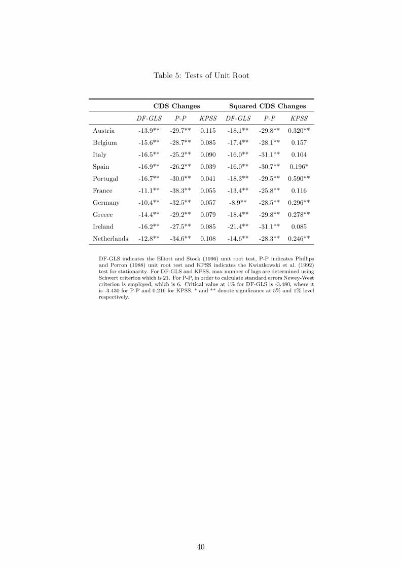
Table 5: Tests of Unit Root
CDS Changes Squared CDS Changes
DF-GLS P-P KPSS DF-GLS P-P KPSS
Austria -13.9** -29.7** 0.115 -18.1** -29.8** 0.320**
Belgium -15.6** -28.7** 0.085 -17.4** -28.1** 0.157
Italy -16.5** -25.2** 0.090 -16.0** -31.1** 0.104
Spain -16.9** -26.2** 0.039 -16.0** -30.7** 0.196*
Portugal -16.7** -30.0** 0.041 -18.3** -29.5** 0.590**
France -11.1** -38.3** 0.055 -13.4** -25.8** 0.116
Germany -10.4** -32.5** 0.057 -8.9** -28.5** 0.296**
Greece -14.4** -29.2** 0.079 -18.4** -29.8** 0.278**
Ireland -16.2** -27.5** 0.085 -21.4** -31.1** 0.085
Netherlands -12.8** -34.6** 0.108 -14.6** -28.3** 0.246**
DF-GLS indicates the Elliott and Stock (1996) unit root test, P-P indicates Phillipsand Perron (1988) unit root test and KPSS indicates the Kwiatkowski et al. (1992)test for stationarity. For DF-GLS and KPSS, max number of lags are determined usingSchwert criterion which is 21. For P-P, in order to calculate standard errors Newey-Westcriterion is employed, which is 6. Critical value at 1% for DF-GLS is -3.480, where itis -3.430 for P-P and 0.216 for KPSS. * and ** denote significance at 5% and 1% levelrespectively.
40

Tab
le6:
Lon
gM
emor
yfo
rP
ost
9A
ugu
st20
07
GPH
MLR
Pan
elA
Spre
ad
Changes
m=
0.5
t-va
lm
=0.
55t-
val
m=
0.60
t-va
lm
=0.
5t-
val
m=
0.55
t-va
lm
=0.
60t-
val
Au
stri
a0.1
731.
31
0.1
761.
650.
127
1.45
0.15
91.
470.
170
1.94
0.12
21.
75B
elgi
um
0.23
91.
810.
192
1.80
0.08
40.
960.
211
1.45
0.17
31.
530.
072
0.84
Ital
y0.
193
1.46
0.13
51.2
70.
012
0.13
0.24
41.
780.
170
1.51
0.03
90.
42S
pai
n0.
118
0.90
0.06
70.6
3-0
.035
-0.4
00.
080
0.56
0.03
00.
29-0
.072
-0.8
6P
ortu
gal
-0.0
02
-0.0
2-0
.014
-0.1
3-0
.057
-0.6
50.
100
0.70
0.05
90.
55-0
.004
-0.0
5F
ran
ce0.
165
1.25
0.189
1.7
70.
140
1.59
0.36
6**
5.08
0.34
9**
4.61
0.26
5**
3.61
Ger
man
y0.
102
0.77
0.149
1.39
0.11
51.
310.
330*
*3.
590.
329*
*3.
640.
252*
*3.
20G
reec
e0.
115
0.87
0.1
821.
700.
059
0.68
0.11
50.
960.
182
2.00
0.06
10.
87Ir
elan
d0.
181
1.37
0.23
3*2.
180.
073
0.83
0.16
61.
220.
219
1.78
0.06
10.
60N
eth
erla
nd
s0.1
781.
34
0.23
6*2.
210.
108
1.23
0.50
5**
5.02
0.50
7**
6.07
0.31
9**
3.81
Pan
elB
Square
dSpre
ad
Changes
m=
0.5
t-va
lm
=0.
55t-
val
m=
0.60
t-va
lm
=0.
5t-
val
m=
0.55
t-va
lm
=0.
60t-
val
Au
stri
a0.2
231.
69
0.1
631.
520.
121
1.38
0.23
81.
320.
175
1.38
0.12
51.
34B
elgi
um
0.2
94*
2.22
0.328
**3.
070.
375*
*4.
260.
322*
*2.
790.
349*
*3.
760.
389*
*5.
40It
aly
0.2
411.
83
0.2
78**
2.60
0.26
4**
3.00
0.27
2**
2.53
0.30
0**
3.77
0.27
9**
4.36
Sp
ain
0.10
60.
800.
110
1.03
0.24
7**
2.81
0.21
81.
980.
196*
*2.
530.
309*
*3.
97P
ortu
gal
0.17
01.
290.
242*
2.27
0.26
4**
3.01
0.15
91.
150.
230*
2.19
0.25
3**
3.04
Fra
nce
0.16
91.
280.
147
1.3
80.
207*
2.36
0.17
61.
210.
152
1.39
0.21
1*2.
47G
erm
any
0.25
91.
960.3
20**
2.99
0.27
6**
3.14
0.31
4*2.
400.
357*
*3.
550.
305*
*4.
07G
reec
e0.
317*
2.40
0.39
5**
3.7
00.
416*
*4.
730.
305*
*3.
920.
384*
*5.
830.
405*
*5.
60Ir
elan
d-0
.107
-0.8
10.
110
1.03
0.06
00.
680.
163
1.49
0.30
5**
2.81
0.21
3*2.
52N
eth
erla
nd
s0.
297*
2.25
0.22
0*2.
060.
160
1.83
0.26
1*2.
200.
191
2.01
0.13
81.
78
Th
ista
ble
show
sth
elo
ng
mem
ory
test
sfo
rsp
read
chan
ges
an
dsq
uare
dsp
read
chan
ges
for
the
per
iod
aft
erA
ugu
st9,2007.
Pan
elA
con
centr
ate
son
spre
ad
chan
ges
,w
hile
Pan
elB
illu
stra
tes
the
lon
gm
emory
esti
mate
sfo
rsq
uare
dsp
read
chan
ges
.T
he
firs
t,th
ird
an
dfi
fth
colu
mn
sof
the
tab
lep
rese
nt
the
GP
Hes
tim
ate
sfo
rp
ow
ervalu
esof
0.5
0,
0.5
5an
d0.6
0,
resp
ecti
vel
y,an
dth
ese
ven
th,
nin
than
del
even
thco
lum
ns
corr
esp
on
dto
the
esti
mate
sof
the
ML
Rfo
rth
esa
me
pow
ervalu
es.
*an
d**
den
ote
sign
ifica
nce
at
5%
an
d1%
level
resp
ecti
vel
y.T
ime
seri
esfo
rea
chco
untr
yco
nta
in1098
data
poin
ts.m
rep
rese
nts
the
pow
ervalu
esem
plo
yed
,w
hic
hareT
0.5
,T0.55
an
dT
0.60
that
corr
esp
on
dto
33,
47
an
d67
ord
inate
s.
41

Tab
le7:
Lon
gM
emor
yfo
rP
ost
Leh
man
Per
iod
GPH
MLR
Pan
elA
Spre
ad
Changes
m=
0.5
t-va
lm
=0.
55t-
val
m=
0.60
t-va
lm
=0.
5t-
val
m=
0.55
t-va
lm
=0.
60t-
val
Au
stri
a0.
080
0.55
0.16
01.
340.
070
0.71
0.10
50.
920.
157
1.35
0.06
90.
77B
elgi
um
0.06
90.4
70.0
850.
72-0
.057
-0.5
80.
199
1.27
0.17
71.
360.
003
0.03
Ital
y0.
006
0.0
4-0
.018
-0.1
5-0
.168
-1.7
20.
011
0.08
-0.0
01-0
.01
-0.1
49-1
.72
Sp
ain
-0.1
93-1
.32
-0.1
51-1
.26
-0.2
41-2
.46
-0.0
03-0
.02
-0.0
15-0
.10
-0.1
48-1
.35
Port
ugal
-0.1
41-0
.97
-0.0
48-0
.40
-0.1
13-1
.15
-0.0
09-0
.11
0.06
00.
68-0
.018
-0.2
1F
ran
ce-0
.048
-0.3
3-0
.040
-0.3
4-0
.135
-1.3
90.
234
1.96
0.21
1*2.
190.
081
1.09
Ger
man
y-0
.085
-0.5
8-0
.040
-0.3
4-0
.058
-0.6
00.
249
2.03
0.20
2*2.
090.
115
1.35
Gre
ece
-0.0
24-0
.17
-0.0
02-0
.02
-0.0
90-0
.92
0.00
60.
040.
014
0.12
-0.0
80-0
.85
Irel
and
0.07
00.
480.
088
0.7
4-0
.033
-0.3
40.
069
0.55
0.08
70.
82-0
.034
-0.3
8N
eth
erla
nd
s0.
231.
60
0.19
51.
630.
048
0.49
0.60
43.
460.
421*
*3.
120.
179
1.59
Pan
elB
Square
dSpre
ad
Changes
m=
0.5
t-va
lm
=0.
55t-
val
m=
0.60
t-va
lm
=0.
5t-
val
m=
0.55
t-va
lm
=0.
60t-
val
Au
stri
a0.
311
2.13
0.270
*2.
260.
236*
2.41
0.33
6**
3.19
0.29
4**
3.47
0.24
3**
3.43
Bel
giu
m0.
365*
*2.
500.
346*
*2.9
00.
418*
*4.
270.
427*
*3.
060.
392*
*3.
900.
446*
*5.
01It
aly
0.15
51.0
60.1
901.
590.
143
1.47
0.28
71.
930.
303*
*2.
720.
236*
*2.
86S
pai
n0.1
621.
110.
220
1.84
0.27
4**
2.81
0.27
5**
3.31
0.30
6**
4.39
0.34
3**
5.48
Por
tuga
l0.1
410.
970.2
39*
2.00
0.24
0*2.
460.
209
1.58
0.28
6**
2.83
0.28
1**
3.47
Fra
nce
0.13
10.
900.
200
1.68
0.30
9**
3.16
0.19
51.
940.
244*
2.54
0.34
7**
3.28
Ger
man
y0.
266
1.8
20.3
39**
2.84
0.36
2**
3.70
0.21
31.
830.
289*
*2.
860.
318*
*3.
80G
reec
e0.
308*
2.11
0.366
**3.
060.
332*
*3.
400.
318*
2.23
0.37
3**
3.39
0.33
8**
3.99
Irel
and
-0.0
18-0
.12
0.09
90.
830.
072
0.74
0.16
51.
490.
241*
*2.
780.
176*
*2.
46N
eth
erla
nd
s0.4
13**
2.83
0.235
*1.
970.
188
1.93
0.42
1**
3.11
0.23
7*2.
050.
186*
2.11
Th
ista
ble
show
sth
elo
ng
mem
ory
test
sfo
rsp
read
chan
ges
an
dsq
uare
dsp
read
chan
ges
for
the
per
iod
aft
erth
ed
efau
ltof
Leh
man
.P
an
elA
con
centr
ate
son
spre
ad
chan
ges
,w
her
eas
Pan
elB
illu
stra
tes
the
lon
gm
emory
esti
mate
sfo
rsq
uare
dsp
read
chan
ges
.T
he
firs
t,th
ird
an
dfi
fth
colu
mn
sof
the
tab
lep
rese
nt
the
GP
Hes
tim
ate
sfo
rp
ow
erle
vel
sof
0.5
0,
0.5
5and
0.6
0,
resp
ecti
vel
yan
dth
ese
ven
th,
nin
thand
elev
enth
colu
mn
sare
the
esti
mate
sof
the
ML
Rfo
rth
esa
me
pow
ervalu
es.
*and
**
den
ote
sign
ifica
nce
at
5%
an
d1%
level
resp
ecti
vel
y.T
ime
seri
esfo
rea
chco
untr
yco
nta
in887
data
poin
ts.m
rep
rese
nts
the
pow
ervalu
esem
plo
yed
,w
hic
hareT
0.5
,T0.55
an
dT
0.60
that
corr
esp
on
dto
30,
42
an
d59
ord
inate
s.
42

Tab
le8:
Dual
Mem
ory
ARFIM
A(2
,ξ,2)-FIG
ARCH(1
,d,1)
µξ
AR
(1)
AR
(2)
MA
(1)
MA
(2)
ωd
ARCH
(1)
GARCH
(1)
Au
stri
a0.
184
-0.0
290.
021
0.33
5-0
.175
-0.2
233.
306
0.3
79
-0.0
03
0.2
55
(0.1
45)
(0.0
79)
(0.3
14)
(0.2
23)
(0.3
26)
(0.2
18)
(3.8
43)
(0.2
39)
(0.4
64)
(0.6
42)
Fra
nce
0.22
90.
037
-0.0
06-0
.147
0.05
60.
112
2.34
70.3
56
0.4
39
0.4
93*
(0.1
75)
(0.0
56)
(0.6
31)
(0.1
22)
(0.6
45)
(0.1
04)
(1.7
21)
(0.2
03)
(0.2
30)
(0.1
99)
Ger
man
y0.
248
0.02
6-0
.422
0.03
70.
437
0.01
90.
945
0.5
59
0.4
60*
0.7
40**
(0.1
49)
(0.0
45)
(0.3
65)
(0.3
22)
(0.3
64)
(0.3
23)
(0.4
29)
(0.3
16)
(0.1
93)
(0.1
22)
Net
her
lan
ds
0.28
6*-0
.088
0.17
20.
660*
*-0
.038
-0.6
68**
3.27
70.5
53
0.2
91
0.4
65
(0.1
45)
(0.1
23)
(0.1
31)
(0.1
11)
(0.1
06)
(0.
102)
(6.9
47)
(0.4
66)
(0.8
69)
(1.1
93)
Bel
giu
m0.
230
-0.1
571.
244*
*-0
.271
-0.8
87**
-0.0
300.
929
0.6
20**
0.2
85
0.7
39**
(0.1
54)
(0.1
48)
(0.1
83)
(0.1
70)
(0.1
03)
(0.0
89)
(0.6
38)
(0.2
15)
(0.1
59)
(0.0
70)
Ital
y0.
220
-0.0
26-0
.175
60.
171
0.46
9**
-0.0
581.
145
0.4
11**
0.0
63
0.2
95
(0.1
21)
(0.0
55)
(0.1
03)
(0.1
15)
(0.1
10)
(0.0
95)
(1.3
62)
(0.1
59)
(0.4
93)
(0.6
07)
Irel
and
0.31
3*-0
.010
-0.1
310.
297*
*0.
369*
-0.1
670.
158
0.7
46**
0.4
17**
0.9
05**
(0.1
51)
(0.0
69)
(0.1
49)
(0.1
11)
(0.1
29)
(0.0
88)
(0.1
35)
(0.1
74)
(0.1
33)
(0.0
48)
Por
tuga
l0.
413*
*-0
.145
0.03
30.
253
0.31
2-0
.121
0.89
1*0.8
38**
-0.0
38
0.7
02**
(0.0
83)
(0.1
05)
(0.2
28)
(0.1
69)
(0.2
44)
(0.0
97)
(0.4
52)
(0.1
26)
(0.0
98)
(0.0
76)
Sp
ain
0.28
30.
079
0.92
9-0
.615
-0.8
200.
523
0.57
30.5
34**
0.2
51*
0.6
23**
(0.1
82)
(0.2
25)
(1.4
89)
(1.2
65)
(1.8
48)
(1.4
10)
(0.4
60)
(0.1
27)
(0.1
12)
(0.1
32)
Gre
ece
0.39
7**
0.02
6-0
.244
0.22
00.
455
-0.1
100.
198*
0.9
92**
0.0
08
0.8
76**
(0.1
46)
(0.0
78)
(0.2
11)
(0.1
62)
(0.1
89)
(0.1
41)
(0.0
93)
(0.1
22)
(0.1
10)
(0.0
40)
Th
ista
ble
pre
sents
the
AR
FIM
A-F
IGA
RC
Hm
odel
coeffi
cien
ts.µ
isth
ees
tim
ate
dco
nst
ant
for
the
mea
neq
uati
on
wh
ereω
isth
eco
nst
ant
for
the
vari
an
ceeq
uati
on
.A
R(1
)an
dA
R(2
)are
the
au
tore
gre
ssiv
ep
ara
met
ers,
wh
erea
sM
A(1
)an
dM
A(2
)are
the
movin
gaver
age
para
met
ers
of
the
AR
FIM
Am
od
el.
Inth
eF
IGA
RC
Hm
od
el,
the
vola
tility
clu
ster
ing
isca
ptu
red
by
AR
CH
(1)
an
dG
AR
CH
(1).
Th
ekey
para
met
ers
of
inte
rest
areξ
an
dd,
wh
ich
are
the
lon
gm
emory
esti
mate
sfo
rA
RF
IMA
an
dF
IGA
RC
Hre
spec
tivel
y.R
ob
ust
stan
dard
erro
rsare
inp
are
nth
eses
.*
an
d**
den
ote
sign
ifica
nce
at
,5%
an
d1%
level
resp
ecti
vel
y.S
pre
ad
chan
ge
seri
esu
sed
at
pre
vio
us
sect
ion
sare
mu
ltip
lied
wit
h100
tosi
mp
lify
the
conver
gen
ceof
likel
ihood
.
43

Tab
le9:
Gra
nge
rC
ausa
lity
Tes
ts
CD
Svola
tility
does
not
Gra
nger-
cause
CD
Ssp
read
Days
AU
BE
GR
GE
RF
RN
TIR
ITP
TSP
555
.64*
9.95
103.
12*
21.4
9*18
.61*
4.76
6.14
76.8
6*25
.30*
35.4
7*
(0.0
0)(0
.08)
(0.0
0)(0
.00)
(0.0
0)(0
.31)
(0.2
9)(0
.00)
(0.0
0)(0
.00)
10
66.1
7*27
.88*
161.
17*
28.3
5*20
.23
12.2
19.
5481
.41*
33.8
2*69
.61*
(0.0
0)(0
.00)
(0.0
0)(0
.00)
(0.0
3)(0
.14)
(0.4
8)(0
.00)
(0.0
0)(0
.00)
opt
60.1
0*10
.08
475.
05*
20.9
0*16
.51*
3.43
6.14
*76
.86*
27.8
0*65
.87*
(0.0
0)(0
.04)
(0.0
0)(0
.00)
(0.0
0)(0
.33)
(0.2
9)(0
.00)
(0.0
0)(0
.00)
CD
Svola
tility
does
not
Gra
nger-
cause
CD
Ssp
read
changes
Days
AU
BE
GR
GE
RF
RN
TIR
ITP
TSP
513
3.67
*15
.00
133.
18*
14.0
555
.20*
7.28
39.6
3*68
.23*
38.1
6*21
.92*
(0.0
0)(0
.01)
(0.0
0)(0
.02)
(0.0
0)(0
.12)
(0.0
0)(0
.00)
(0.0
0)(0
.00)
10
139.
89*
47.8
3*19
2.15
*20
.76
66.5
6*12
.09
54.8
0*66
.19*
42.6
4*66
.19*
(0.0
0)(0
.00)
(0.0
0)(0
.02)
(0.0
0)(0
.15)
(0.0
0)(0
.00)
(0.0
0)(0
.00)
opt
125.
14*
13.1
1*13
.11*
11.8
654
.99*
5.33
39.6
3*59
.67*
33.8
2*59
.67*
(0.0
0)(0
.00)
(0.0
0)(0
.01)
(0.0
0)(0
.15)
(0.0
0)(0
.00)
(0.0
0)(0
.00)
Th
ista
ble
pre
sents
the
esti
mate
sof
Gra
nger
-cau
sality
test
.D
ays
rep
rese
nt
the
nu
mb
erof
lags
tob
ein
clu
ded
inth
eb
ivari
ate
Gra
nger
cau
sality
test
.p
-valu
esare
pre
sente
din
pare
nth
eses
.*
ind
icate
ssi
gn
ifica
nce
at
1%
level
.
44
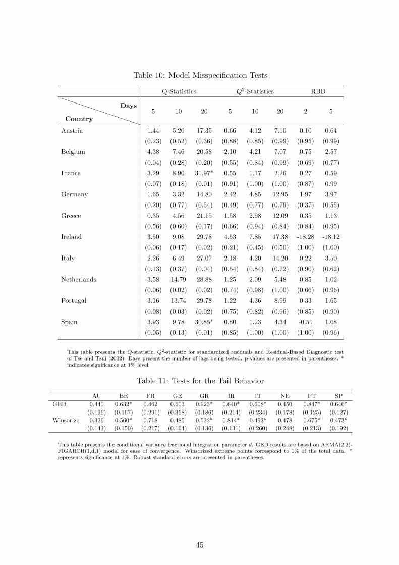
Table 10: Model Misspecification Tests
Q-Statistics Q2-Statistics RBD
Country
Days5 10 20 5 10 20 2 5
Austria 1.44 5.20 17.35 0.66 4.12 7.10 0.10 0.64
(0.23) (0.52) (0.36) (0.88) (0.85) (0.99) (0.95) (0.99)
Belgium 4.38 7.46 20.58 2.10 4.21 7.07 0.75 2.57
(0.04) (0.28) (0.20) (0.55) (0.84) (0.99) (0.69) (0.77)
France 3.29 8.90 31.97* 0.55 1.17 2.26 0.27 0.59
(0.07) (0.18) (0.01) (0.91) (1.00) (1.00) (0.87) 0.99
Germany 1.65 3.32 14.80 2.42 4.85 12.95 1.97 3.97
(0.20) (0.77) (0.54) (0.49) (0.77) (0.79) (0.37) (0.55)
Greece 0.35 4.56 21.15 1.58 2.98 12.09 0.35 1.13
(0.56) (0.60) (0.17) (0.66) (0.94) (0.84) (0.84) (0.95)
Ireland 3.50 9.08 29.78 4.53 7.85 17.38 -18.28 -18.12
(0.06) (0.17) (0.02) (0.21) (0.45) (0.50) (1.00) (1.00)
Italy 2.26 6.49 27.07 2.18 4.20 14.20 0.22 3.50
(0.13) (0.37) (0.04) (0.54) (0.84) (0.72) (0.90) (0.62)
Netherlands 3.58 14.79 28.88 1.25 2.09 5.48 0.85 1.02
(0.06) (0.02) (0.02) (0.74) (0.98) (1.00) (0.66) (0.96)
Portugal 3.16 13.74 29.78 1.22 4.36 8.99 0.33 1.65
(0.08) (0.03) (0.02) (0.75) (0.82) (0.96) (0.85) (0.90)
Spain 3.93 9.78 30.85* 0.80 1.23 4.34 -0.51 1.08
(0.05) (0.13) (0.01) (0.85) (1.00) (1.00) (1.00) (0.96)
This table presents the Q-statistic, Q2-statistic for standardized residuals and Residual-Based Diagnostic testof Tse and Tsui (2002). Days present the number of lags being tested. p-values are presented in parentheses. *indicates significance at 1% level.
Table 11: Tests for the Tail Behavior
AU BE FR GE GR IR IT NE PT SP
GED 0.440 0.632* 0.462 0.603 0.923* 0.640* 0.608* 0.450 0.847* 0.646*
(0.196) (0.167) (0.291) (0.368) (0.186) (0.214) (0.234) (0.178) (0.125) (0.127)
Winsorize 0.326 0.560* 0.718 0.485 0.532* 0.814* 0.492* 0.478 0.675* 0.473*
(0.143) (0.150) (0.217) (0.164) (0.136) (0.131) (0.260) (0.248) (0.213) (0.192)
This table presents the conditional variance fractional integration parameter d. GED results are based on ARMA(2,2)-FIGARCH(1,d,1) model for ease of convergence. Winsorized extreme points correspond to 1% of the total data. *represents significance at 1%. Robust standard errors are presented in parentheses.
45
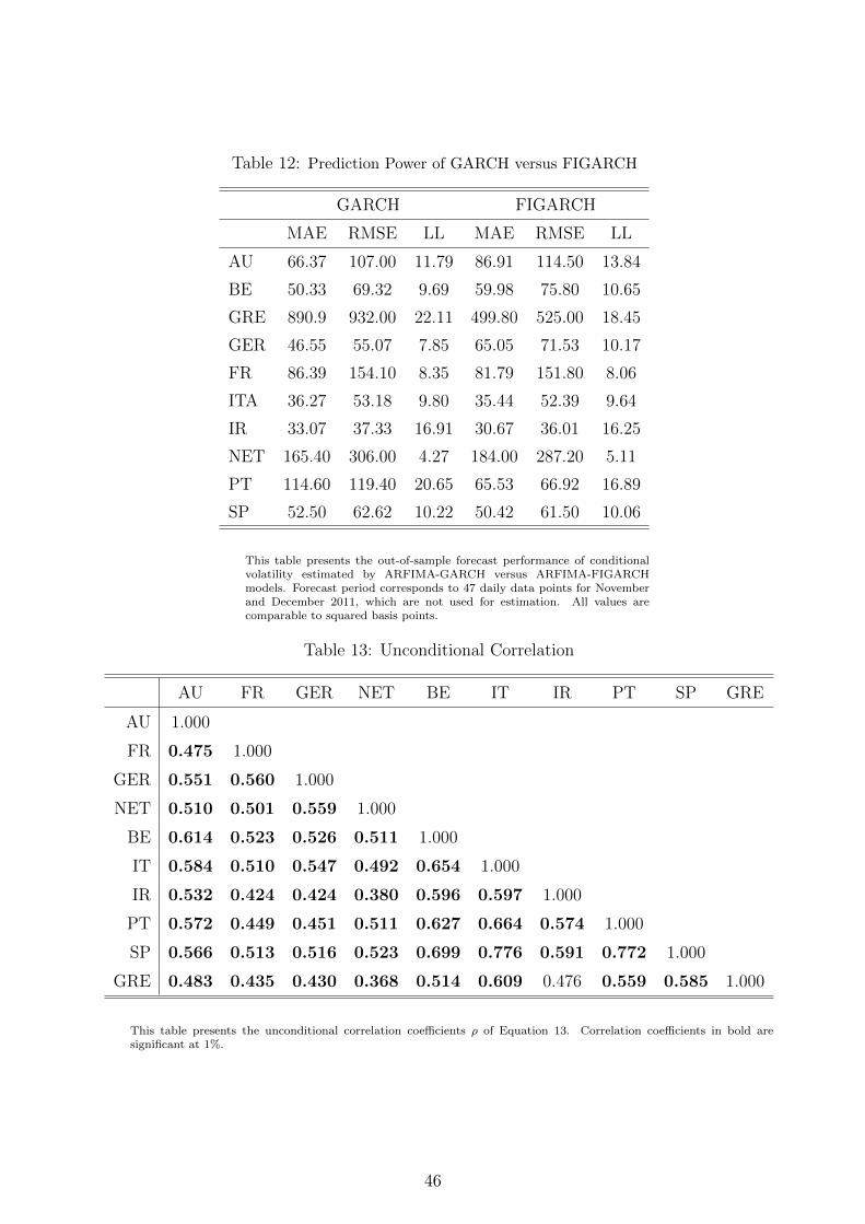
Table 12: Prediction Power of GARCH versus FIGARCH
GARCH FIGARCH
MAE RMSE LL MAE RMSE LL
AU 66.37 107.00 11.79 86.91 114.50 13.84
BE 50.33 69.32 9.69 59.98 75.80 10.65
GRE 890.9 932.00 22.11 499.80 525.00 18.45
GER 46.55 55.07 7.85 65.05 71.53 10.17
FR 86.39 154.10 8.35 81.79 151.80 8.06
ITA 36.27 53.18 9.80 35.44 52.39 9.64
IR 33.07 37.33 16.91 30.67 36.01 16.25
NET 165.40 306.00 4.27 184.00 287.20 5.11
PT 114.60 119.40 20.65 65.53 66.92 16.89
SP 52.50 62.62 10.22 50.42 61.50 10.06
This table presents the out-of-sample forecast performance of conditionalvolatility estimated by ARFIMA-GARCH versus ARFIMA-FIGARCHmodels. Forecast period corresponds to 47 daily data points for Novemberand December 2011, which are not used for estimation. All values arecomparable to squared basis points.
Table 13: Unconditional Correlation
AU FR GER NET BE IT IR PT SP GRE
AU 1.000
FR 0.475 1.000
GER 0.551 0.560 1.000
NET 0.510 0.501 0.559 1.000
BE 0.614 0.523 0.526 0.511 1.000
IT 0.584 0.510 0.547 0.492 0.654 1.000
IR 0.532 0.424 0.424 0.380 0.596 0.597 1.000
PT 0.572 0.449 0.451 0.511 0.627 0.664 0.574 1.000
SP 0.566 0.513 0.516 0.523 0.699 0.776 0.591 0.772 1.000
GRE 0.483 0.435 0.430 0.368 0.514 0.609 0.476 0.559 0.585 1.000
This table presents the unconditional correlation coefficients ρ of Equation 13. Correlation coefficients in bold aresignificant at 1%.
46

Table 14: Recent Comovements
AU FR GER NET BE IT IR PT SP GRE
AU 1.000
FR 0.015 1.000
GER 0.020 0.050 1.000
NET 0.023 0.038 0.029 1.000
BE 0.096 0.036 0.056 0.019 1.000
IT 0.094 0.018 0.017 0.069 0.018 1.000
IR 0.000 0.013 0.028 0.021 0.019 0.026 1.000
PT 0.059 0.024 0.026 0.019 0.019 0.021 0.017 1.000
SP 0.071 0.135 0.051 0.016 0.104 0.116 0.024 0.056 1.000
GRE 0.001 0.054 0.040 0.017 0.023 0.017 0.025 0.021 0.103 1.000
This table presents the recent comovement coefficients α of Equation 13. Coefficients in bold are significant at 1%.
Table 15: Persistent Comovements
AU FR GER NET BE IT IR PT SP GRE
AU 1.000
FR 0.515 1.000
GER 0.966 0.927 1.000
NET 0.962 0.938 0.957 1.000
BE 0.453 0.881 0.839 0.949 1.000
IT 0.404 0.762 0.958 0.968 0.819 1.000
IR 0.760 0.939 0.917 0.962 0.946 0.946 1.000
PT 0.000 0.964 0.951 0.967 0.948 0.939 0.969 1.000
SP 0.726 0.355 0.885 0.969 0.787 0.686 0.943 0.922 1.000
GRE 0.984 0.854 0.826 0.972 0.906 0.970 0.964 0.947 0.649 1.000
This table presents the persistent comovement coefficients β of Equation 13. Coefficients in bold are significant at 1%.
47

Fig
ure
3:Sel
ecte
dP
airw
ise
Dynam
icC
ondit
ional
Cor
rela
tion
sfo
rG
reec
e
Gre
ece
vs G
erm
any
2008
2009
2010
2011
2012
0.1
0.2
0.3
0.4
0.5
0.6
0.7
0.8
0.9
1.0
Gre
ece
vs G
erm
any
(a)
Gre
ece
vs
Ger
many
Gre
ece
vs I
taly
2008
2009
2010
2011
2012
0.1
0.2
0.3
0.4
0.5
0.6
0.7
0.8
0.9
1.0
Gre
ece
vs I
taly
(b)
Gre
ece
vs
Ital
y
Gre
ece
vs S
pain
2008
2009
2010
2011
2012
0.1
0.2
0.3
0.4
0.5
0.6
0.7
0.8
0.9
1.0
Gre
ece
vs S
pain
(c)
Gre
ece
vs
Sp
ain
Gre
ece
vs P
ortu
gal
2008
2009
2010
2011
2012
0.1
0.2
0.3
0.4
0.5
0.6
0.7
0.8
0.9
1.0
Gre
ece
vs P
ortu
gal
(d)
Gre
ece
vs
Por
tuga
l
48