portfolio diversi cation in the sovereign credit swap …...2016/11/16 · portfolio diversi cation...
TRANSCRIPT
Portfolio diversificationin the sovereign credit swap markets
Andrea Consiglio ∗
Somayyeh Lotfi †
Stavros A. Zenios ‡
July 2016.
Working Paper 16-06The Wharton Financial Institutions Center
The Wharton School, University of Pennsylvania, PA
Abstract
We develop models for portfolio diversification in the sovereign credit defaultswap (CDS) markets and show that, despite literature findings that sovereign CDSspreads are affected by global factors, there is sufficient idiosyncratic risk to bediversified away. However, we identify regime switching in the times series of CDSspreads, and the portfolio diversification strategies may differ between regimes. Themodels trade off the CVaR risk measure against expected return. They are testedin an active management setting for Eurozone core, periphery, and Central, Easternand South-Eastern Europe (CESEE) countries. Models are developed for investorswith long positions in CDS, speculators that hold uncovered long and short po-sitions, and hedgers with covered long and short exposures. The results comparefavorably with the broad S&P/ISDA Eurozone Developed Nation Sovereign CDSindex. We also identify several issues that remain unexplored on the way to devel-oping integrated risk management models for CDS portfolios.
Keywords: Credit derivatives; portfolio diversification; Eurozone crisis; CDS spreads;Conditional Value-at-Risk; regime switching.
∗Department of Economics, Management and Statistics, University of Palermo, Palermo, IT. [email protected]†Department of Applied Mathematics, University of Guilan, Rasht, Iran. [email protected]‡Department of Accounting and Finance, University of Cyprus, Nicosia, CY, Norwegian School
of Economics, and Wharton Financial Institutions Center, University of Pennsylvania, [email protected]
1
Contents
1 Introduction 3
2 Some empirical analysis of sovereign CDS markets 52.1 Regime switching . . . . . . . . . . . . . . . . . . . . . . . . . . . . . . . 52.2 Common regime breaks . . . . . . . . . . . . . . . . . . . . . . . . . . . . 11
3 The CVaR portfolio optimization models 123.1 Long exposures . . . . . . . . . . . . . . . . . . . . . . . . . . . . . . . . 133.2 Uncovered long and short exposures . . . . . . . . . . . . . . . . . . . . . 133.3 Covered long and short exposures . . . . . . . . . . . . . . . . . . . . . . 14
4 Portfolio diversification 154.1 Diversification pays . . . . . . . . . . . . . . . . . . . . . . . . . . . . . . 154.2 Diversification is regime dependent . . . . . . . . . . . . . . . . . . . . . 16
5 Active portfolio management 19
6 Conclusions 20
Acknowledgements
Stavros Zenios is holder of a Marie Sklodowska-Curie fellowship funded from the European
Union Horizon 2020 research and innovation programme under Marie Sklodowska-Curie grant
agreement No 655092.
2
1 Introduction
In this paper we take a portfolio view of sovereign credit default swaps, contributingto the extensive literature of credit default swaps (CDS) pricing the natural extensionfrom individual instruments to portfolios. Sovereign CDS are insurance contracts offeringprotection against the default of a referenced sovereign government. They emerged in the1990’s as a significant credit derivative security in the sovereign debt market. Their raisond’etre is to hedge and trade sovereign credit risks. They offer investors the opportunity totake a view purely on credit. They are used by sovereign debt investors to hedge againstlosses from a default or other credit event of the sovereign. Speculators take nakedpositions in these instruments —without buying the underlying asset— to place a bet onthe credit risk of the reference entity. Arbitrageurs exploit price differences between thederivative and the underlying debt obligation(s) by taking offsetting positions in the two.
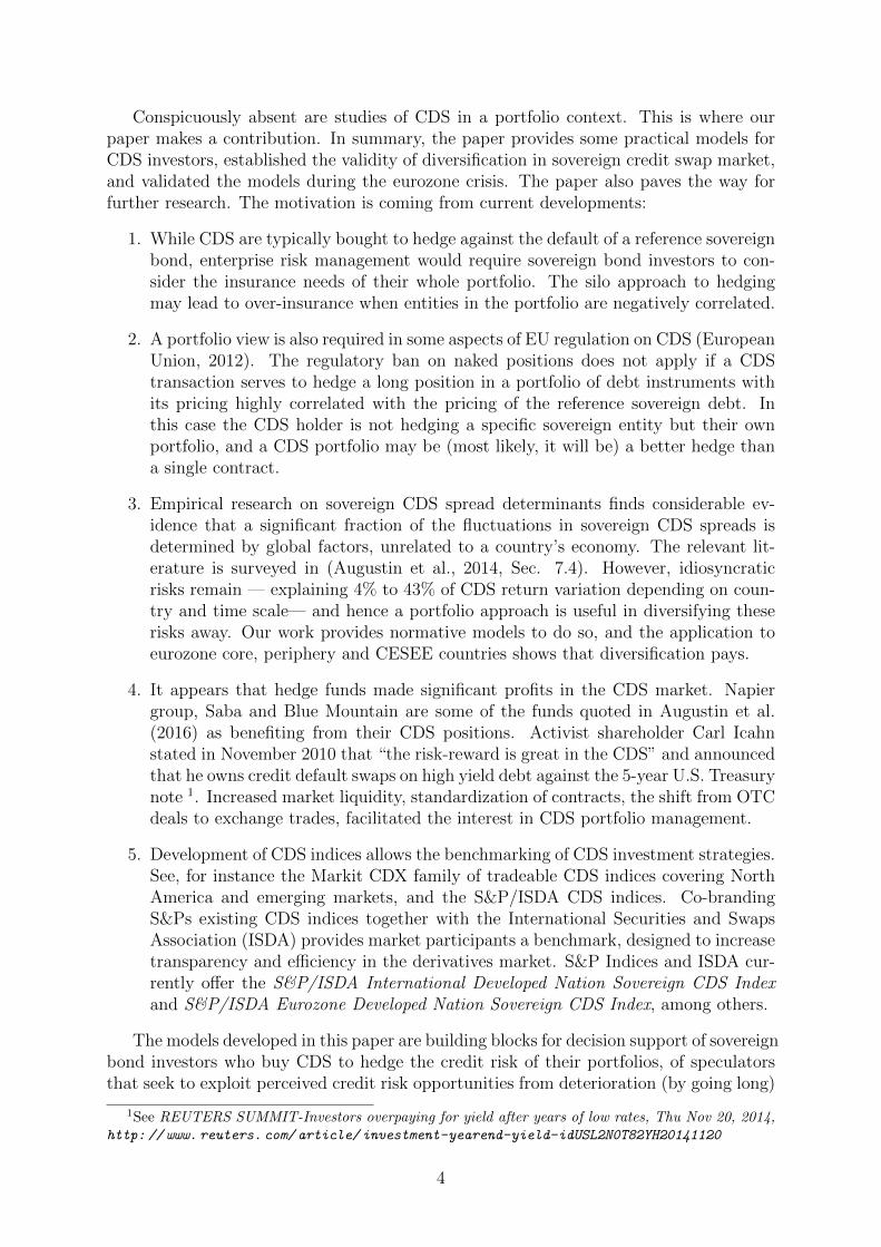
Following standardization of CDS contracts in 1998-1999 and successful execution ina few defaults —starting with Argentina in 2001— the market grew rapidly. Packer andSuthiphongchai (2003) discuss the early developments and Figure 1 illustrates the marketgrowth since 2005 when BIS started publishing data. We report notional amounts andgross market value together with the number of dealers. Notional amounts provide ameasure of market size, but gross market values —whereby open contracts are netted outat market prices— better reflect the scale of risk transfer in the market.
CDS have been criticized for facilitating market manipulations in the eurozone crisis.Naked trading was banned by the German financial regulator in May 2010 and by theEU since November 2012, despite the findings of a European Commission report, Criadoet al. (2010). More recently IMF (2013) presented evidence that refutes the criticismagainst their use and argues that CDS have contributed to the deepening and efficiencyof the sovereign markets. A nuanced view on the role of credit default swaps in the creditcrisis of 2008 is offered by Stulz (2010) who argues that “financial derivatives have clearlylost any presumption of innocence” but finds it would be misguided “to turn 180 degreesfrom a presumption of innocence to a presumption of guilt”.
Figure 1: The growing market for sovereign Credit Default Swaps.(Source: Bank for International Settlement and authors’ calculations.)
The CDS markets, the statistical properties of CDS spreads, spread returns and spreadterm structures, the price discovery mechanisms and market spillovers have been studiedextensively. The corporate CDS market gets the lion’s share of research, but attentionfocused recently on the sovereign market as well. We do not review the extensive extantbody of knowledge here and refer readers to the survey and discussion on future prospects,Augustin et al. (2014, 2016), and recent work on sovereign CDS, Fabozzi et al. (2016).
3
Conspicuously absent are studies of CDS in a portfolio context. This is where ourpaper makes a contribution. In summary, the paper provides some practical models forCDS investors, established the validity of diversification in sovereign credit swap market,and validated the models during the eurozone crisis. The paper also paves the way forfurther research. The motivation is coming from current developments:
1. While CDS are typically bought to hedge against the default of a reference sovereignbond, enterprise risk management would require sovereign bond investors to con-sider the insurance needs of their whole portfolio. The silo approach to hedgingmay lead to over-insurance when entities in the portfolio are negatively correlated.
2. A portfolio view is also required in some aspects of EU regulation on CDS (EuropeanUnion, 2012). The regulatory ban on naked positions does not apply if a CDStransaction serves to hedge a long position in a portfolio of debt instruments withits pricing highly correlated with the pricing of the reference sovereign debt. Inthis case the CDS holder is not hedging a specific sovereign entity but their ownportfolio, and a CDS portfolio may be (most likely, it will be) a better hedge thana single contract.
3. Empirical research on sovereign CDS spread determinants finds considerable ev-idence that a significant fraction of the fluctuations in sovereign CDS spreads isdetermined by global factors, unrelated to a country’s economy. The relevant lit-erature is surveyed in (Augustin et al., 2014, Sec. 7.4). However, idiosyncraticrisks remain — explaining 4% to 43% of CDS return variation depending on coun-try and time scale— and hence a portfolio approach is useful in diversifying theserisks away. Our work provides normative models to do so, and the application toeurozone core, periphery and CESEE countries shows that diversification pays.
4. It appears that hedge funds made significant profits in the CDS market. Napiergroup, Saba and Blue Mountain are some of the funds quoted in Augustin et al.(2016) as benefiting from their CDS positions. Activist shareholder Carl Icahnstated in November 2010 that “the risk-reward is great in the CDS” and announcedthat he owns credit default swaps on high yield debt against the 5-year U.S. Treasurynote 1. Increased market liquidity, standardization of contracts, the shift from OTCdeals to exchange trades, facilitated the interest in CDS portfolio management.
5. Development of CDS indices allows the benchmarking of CDS investment strategies.See, for instance the Markit CDX family of tradeable CDS indices covering NorthAmerica and emerging markets, and the S&P/ISDA CDS indices. Co-brandingS&Ps existing CDS indices together with the International Securities and SwapsAssociation (ISDA) provides market participants a benchmark, designed to increasetransparency and efficiency in the derivatives market. S&P Indices and ISDA cur-rently offer the S&P/ISDA International Developed Nation Sovereign CDS Indexand S&P/ISDA Eurozone Developed Nation Sovereign CDS Index, among others.
The models developed in this paper are building blocks for decision support of sovereignbond investors who buy CDS to hedge the credit risk of their portfolios, of speculatorsthat seek to exploit perceived credit risk opportunities from deterioration (by going long)
1See REUTERS SUMMIT-Investors overpaying for yield after years of low rates, Thu Nov 20, 2014,http: // www. reuters. com/ article/ investment-yearend-yield-idUSL2N0T82YH20141120
4
or improvements (by going short) of a sovereign’s credit rating, and of dealers that bothbuy and sell CDS and wish to have a covered portfolio exposure. The paper is orga-nized as follows: Section 2 reports statistical analysis of the sovereign CDS markets andidentifies regime switching, Section 3 formulates the models, and Sections 4 and 5 re-port results with portfolio diversification and active portfolio management, respectively.Section 6 draws conclusions.
2 Some empirical analysis of sovereign CDS markets
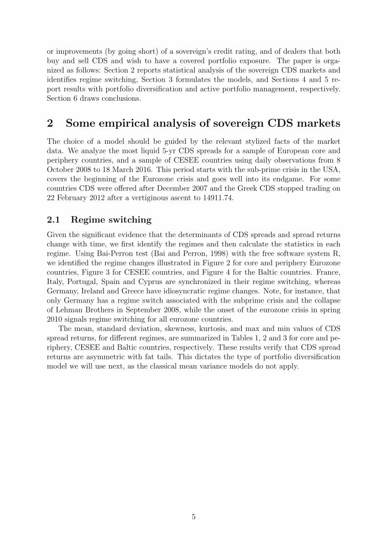
The choice of a model should be guided by the relevant stylized facts of the marketdata. We analyze the most liquid 5-yr CDS spreads for a sample of European core andperiphery countries, and a sample of CESEE countries using daily observations from 8October 2008 to 18 March 2016. This period starts with the sub-prime crisis in the USA,covers the beginning of the Eurozone crisis and goes well into its endgame. For somecountries CDS were offered after December 2007 and the Greek CDS stopped trading on22 February 2012 after a vertiginous ascent to 14911.74.
2.1 Regime switching
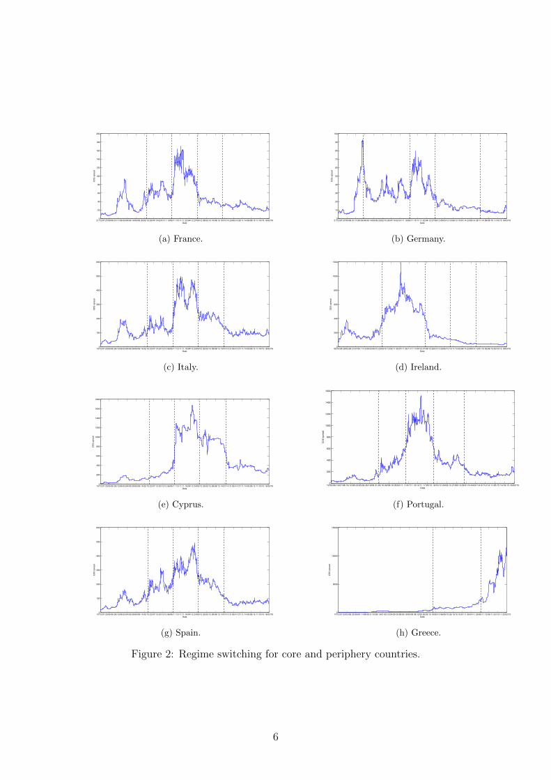
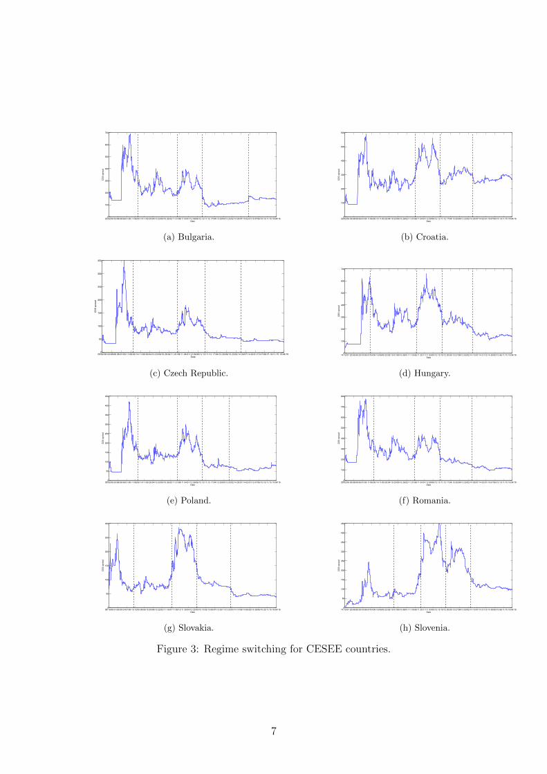
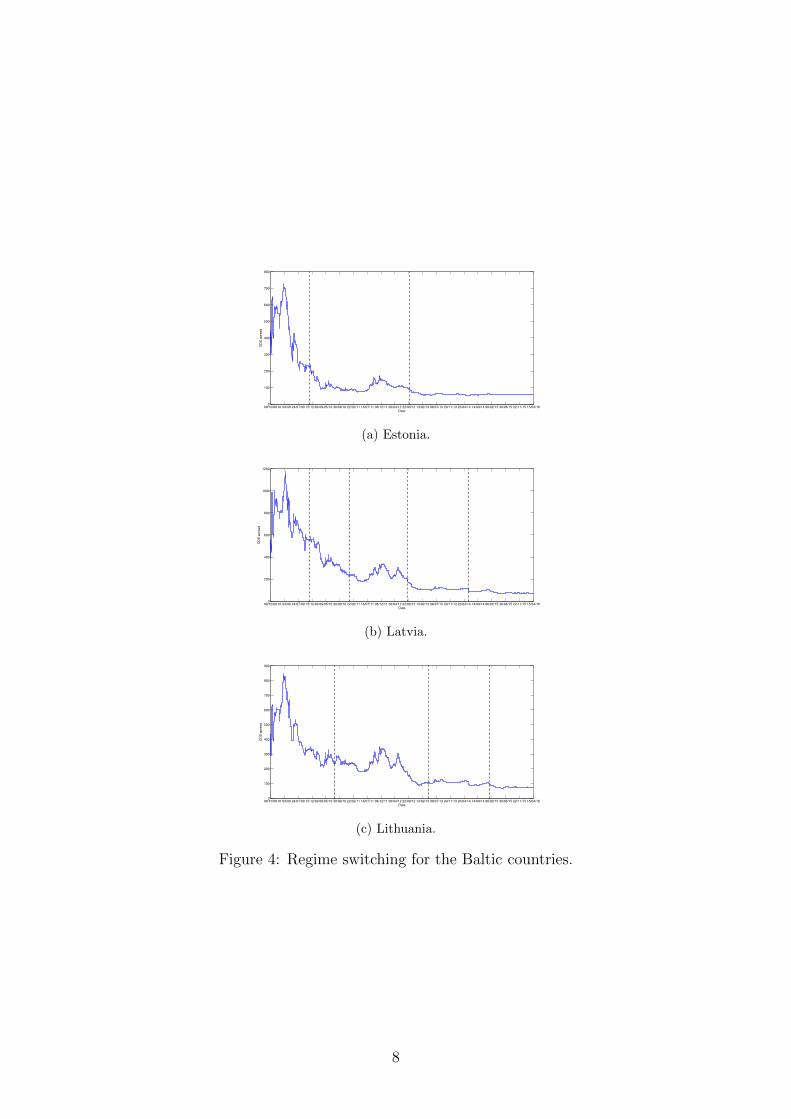
Given the significant evidence that the determinants of CDS spreads and spread returnschange with time, we first identify the regimes and then calculate the statistics in eachregime. Using Bai-Perron test (Bai and Perron, 1998) with the free software system R,we identified the regime changes illustrated in Figure 2 for core and periphery Eurozonecountries, Figure 3 for CESEE countries, and Figure 4 for the Baltic countries. France,Italy, Portugal, Spain and Cyprus are synchronized in their regime switching, whereasGermany, Ireland and Greece have idiosyncratic regime changes. Note, for instance, thatonly Germany has a regime switch associated with the subprime crisis and the collapseof Lehman Brothers in September 2008, while the onset of the eurozone crisis in spring2010 signals regime switching for all eurozone countries.
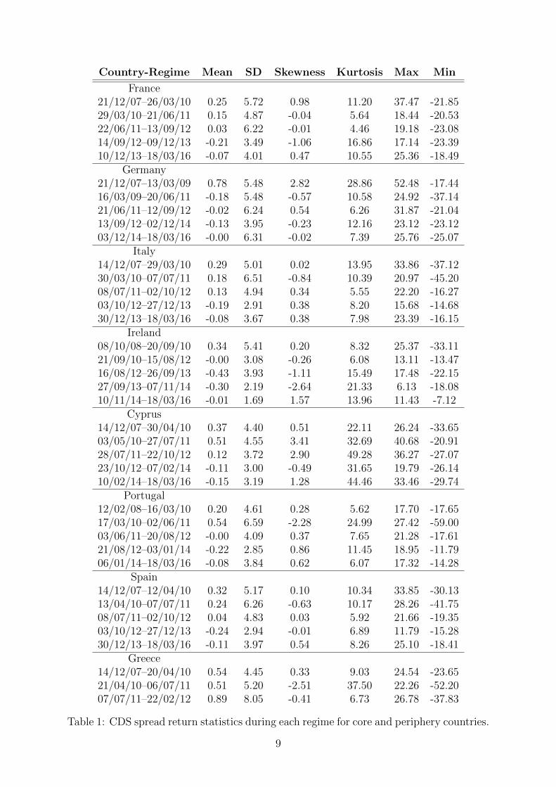
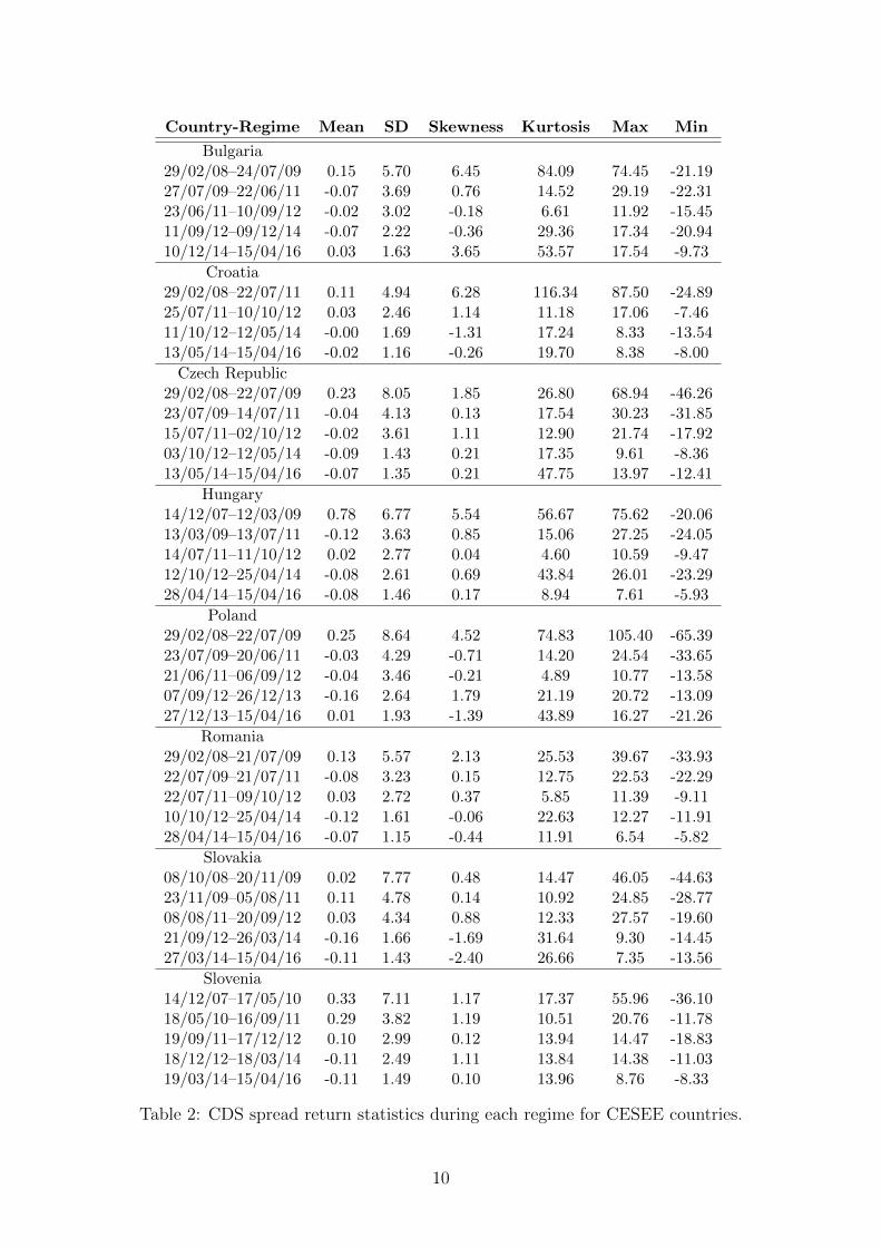
The mean, standard deviation, skewness, kurtosis, and max and min values of CDSspread returns, for different regimes, are summarized in Tables 1, 2 and 3 for core and pe-riphery, CESEE and Baltic countries, respectively. These results verify that CDS spreadreturns are asymmetric with fat tails. This dictates the type of portfolio diversificationmodel we will use next, as the classical mean variance models do not apply.
5
21/12/07 27/05/08 01/11/08 09/04/09 14/09/09 20/02/10 28/07/10 02/01/11 10/06/11 15/11/11 22/04/12 27/09/12 05/03/13 10/08/13 15/01/14 23/06/14 28/11/14 06/05/15 11/10/15 18/03/160
20
40
60
80
100
120
140
160
180
200
CD
S s
pre
ad
Date
(a) France.
21/12/07 27/05/08 01/11/08 09/04/09 14/09/09 20/02/10 28/07/10 02/01/11 10/06/11 15/11/11 22/04/12 27/09/12 05/03/13 10/08/13 15/01/14 23/06/14 28/11/14 06/05/15 11/10/15 18/03/160
10
20
30
40
50
60
70
80
90
100
CD
S s
pre
ad
Date
(b) Germany.
14/12/07 20/05/08 26/10/08 03/04/09 09/09/09 14/02/10 23/07/10 29/12/10 06/06/11 12/11/11 18/04/12 24/09/12 02/03/13 08/08/13 14/01/14 21/06/14 27/11/14 05/05/15 11/10/15 18/03/160
100
200
300
400
500
600
CD
S s
pre
ad
Date
(c) Italy.
08/10/08 28/02/09 21/07/09 11/12/09 03/05/10 23/09/10 13/02/11 06/07/11 26/11/11 17/04/12 07/09/12 28/01/13 20/06/13 10/11/13 02/04/14 23/08/14 13/01/15 05/06/15 26/10/15 18/03/160
200
400
600
800
1000
1200
CD
S s
pre
ad
Date
(d) Ireland.
14/12/07 20/05/08 26/10/08 03/04/09 09/09/09 14/02/10 23/07/10 29/12/10 06/06/11 12/11/11 18/04/12 24/09/12 02/03/13 08/08/13 14/01/14 21/06/14 27/11/14 05/05/15 11/10/15 18/03/160
200
400
600
800
1000
1200
1400
1600
1800
CD
S s
pre
ad
Date
(e) Cyprus.
12/02/08 16/07/08 19/12/08 23/05/09 26/10/09 31/03/10 02/09/10 05/02/11 11/07/11 13/12/11 17/05/12 19/10/12 24/03/13 27/08/13 29/01/14 04/07/14 07/12/14 11/05/15 14/10/15 18/03/160
200
400
600
800
1000
1200
1400
1600
CD
S s
pre
ad
Date
(f) Portugal.
14/12/07 20/05/08 26/10/08 03/04/09 09/09/09 14/02/10 23/07/10 29/12/10 06/06/11 12/11/11 18/04/12 24/09/12 02/03/13 08/08/13 14/01/14 21/06/14 27/11/14 05/05/15 11/10/15 18/03/160
100
200
300
400
500
600
CD
S s
pre
ad
Date
(g) Spain.
14/12/07 03/03/08 23/05/08 11/08/08 31/10/08 19/01/09 10/04/09 30/06/09 18/09/09 08/12/09 26/02/10 18/05/10 06/08/10 26/10/10 15/01/11 05/04/11 25/06/11 13/09/11 03/12/11 22/02/120
5000
10000
15000
CD
S s
pre
ad
Date
(h) Greece.
Figure 2: Regime switching for core and periphery countries.
6
29/02/08 03/08/08 06/01/09 11/06/09 14/11/09 20/04/10 23/09/10 26/02/11 01/08/11 04/01/12 09/06/12 12/11/12 17/04/13 20/09/13 23/02/14 30/07/14 02/01/15 07/06/15 10/11/15 15/04/160
100
200
300
400
500
600
700
CD
S s
pre
ad
Date
(a) Bulgaria.
29/02/08 03/08/08 06/01/09 11/06/09 14/11/09 20/04/10 23/09/10 26/02/11 01/08/11 04/01/12 09/06/12 12/11/12 17/04/13 20/09/13 23/02/14 30/07/14 02/01/15 07/06/15 10/11/15 15/04/160
100
200
300
400
500
600
CD
S s
pre
ad
Date
(b) Croatia.
29/02/08 03/08/08 06/01/09 11/06/09 14/11/09 20/04/10 23/09/10 26/02/11 01/08/11 04/01/12 09/06/12 12/11/12 17/04/13 20/09/13 23/02/14 30/07/14 02/01/15 07/06/15 10/11/15 15/04/160
50
100
150
200
250
300
350
CD
S s
pre
ad
Date
(c) Czech Republic.
14/12/07 22/05/08 29/10/08 07/04/09 15/09/09 22/02/10 01/08/10 08/01/11 18/06/11 25/11/11 03/05/12 10/10/12 20/03/13 27/08/13 03/02/14 13/07/14 21/12/14 30/05/15 06/11/15 15/04/160
100
200
300
400
500
600
700
CD
S s
pre
ad
Date
(d) Hungary.
29/02/08 03/08/08 06/01/09 11/06/09 14/11/09 20/04/10 23/09/10 26/02/11 01/08/11 04/01/12 09/06/12 12/11/12 17/04/13 20/09/13 23/02/14 30/07/14 02/01/15 07/06/15 10/11/15 15/04/160
50
100
150
200
250
300
350
400
450
CD
S s
pre
ad
Date
(e) Poland.
29/02/08 03/08/08 06/01/09 11/06/09 14/11/09 20/04/10 23/09/10 26/02/11 01/08/11 04/01/12 09/06/12 12/11/12 17/04/13 20/09/13 23/02/14 30/07/14 02/01/15 07/06/15 10/11/15 15/04/160
100
200
300
400
500
600
700
800
CD
S s
pre
ad
Date
(f) Romania.
08/10/08 01/03/09 24/07/09 15/12/09 09/05/10 30/09/10 22/02/11 16/07/11 08/12/11 30/04/12 22/09/12 13/02/13 08/07/13 29/11/13 23/04/14 14/09/14 06/02/15 30/06/15 22/11/15 15/04/160
50
100
150
200
250
300
CD
S s
pre
ad
Date
(g) Slovakia.
14/12/07 22/05/08 29/10/08 07/04/09 15/09/09 22/02/10 01/08/10 08/01/11 18/06/11 25/11/11 03/05/12 10/10/12 20/03/13 27/08/13 03/02/14 13/07/14 21/12/14 30/05/15 06/11/15 15/04/160
50
100
150
200
250
300
350
400
450
CD
S s
pre
ad
Date
(h) Slovenia.
Figure 3: Regime switching for CESEE countries.
7
08/10/08 01/03/09 24/07/09 15/12/09 09/05/10 30/09/10 22/02/11 16/07/11 08/12/11 30/04/12 22/09/12 13/02/13 08/07/13 29/11/13 23/04/14 14/09/14 06/02/15 30/06/15 22/11/15 15/04/160
100
200
300
400
500
600
700
800
CD
S s
pre
ad
Date
(a) Estonia.
08/10/08 01/03/09 24/07/09 15/12/09 09/05/10 30/09/10 22/02/11 16/07/11 08/12/11 30/04/12 22/09/12 13/02/13 08/07/13 29/11/13 23/04/14 14/09/14 06/02/15 30/06/15 22/11/15 15/04/160
200
400
600
800
1000
1200
CD
S s
pre
ad
Date
(b) Latvia.
08/10/08 01/03/09 24/07/09 15/12/09 09/05/10 30/09/10 22/02/11 16/07/11 08/12/11 30/04/12 22/09/12 13/02/13 08/07/13 29/11/13 23/04/14 14/09/14 06/02/15 30/06/15 22/11/15 15/04/160
100
200
300
400
500
600
700
800
900
CD
S s
pre
ad
Date
(c) Lithuania.
Figure 4: Regime switching for the Baltic countries.
8
Country-Regime Mean SD Skewness Kurtosis Max Min
France21/12/07–26/03/10 0.25 5.72 0.98 11.20 37.47 -21.8529/03/10–21/06/11 0.15 4.87 -0.04 5.64 18.44 -20.5322/06/11–13/09/12 0.03 6.22 -0.01 4.46 19.18 -23.0814/09/12–09/12/13 -0.21 3.49 -1.06 16.86 17.14 -23.3910/12/13–18/03/16 -0.07 4.01 0.47 10.55 25.36 -18.49
Germany21/12/07–13/03/09 0.78 5.48 2.82 28.86 52.48 -17.4416/03/09–20/06/11 -0.18 5.48 -0.57 10.58 24.92 -37.1421/06/11–12/09/12 -0.02 6.24 0.54 6.26 31.87 -21.0413/09/12–02/12/14 -0.13 3.95 -0.23 12.16 23.12 -23.1203/12/14–18/03/16 -0.00 6.31 -0.02 7.39 25.76 -25.07
Italy14/12/07–29/03/10 0.29 5.01 0.02 13.95 33.86 -37.1230/03/10–07/07/11 0.18 6.51 -0.84 10.39 20.97 -45.2008/07/11–02/10/12 0.13 4.94 0.34 5.55 22.20 -16.2703/10/12–27/12/13 -0.19 2.91 0.38 8.20 15.68 -14.6830/12/13–18/03/16 -0.08 3.67 0.38 7.98 23.39 -16.15
Ireland08/10/08–20/09/10 0.34 5.41 0.20 8.32 25.37 -33.1121/09/10–15/08/12 -0.00 3.08 -0.26 6.08 13.11 -13.4716/08/12–26/09/13 -0.43 3.93 -1.11 15.49 17.48 -22.1527/09/13–07/11/14 -0.30 2.19 -2.64 21.33 6.13 -18.0810/11/14–18/03/16 -0.01 1.69 1.57 13.96 11.43 -7.12
Cyprus14/12/07–30/04/10 0.37 4.40 0.51 22.11 26.24 -33.6503/05/10–27/07/11 0.51 4.55 3.41 32.69 40.68 -20.9128/07/11–22/10/12 0.12 3.72 2.90 49.28 36.27 -27.0723/10/12–07/02/14 -0.11 3.00 -0.49 31.65 19.79 -26.1410/02/14–18/03/16 -0.15 3.19 1.28 44.46 33.46 -29.74
Portugal12/02/08–16/03/10 0.20 4.61 0.28 5.62 17.70 -17.6517/03/10–02/06/11 0.54 6.59 -2.28 24.99 27.42 -59.0003/06/11–20/08/12 -0.00 4.09 0.37 7.65 21.28 -17.6121/08/12–03/01/14 -0.22 2.85 0.86 11.45 18.95 -11.7906/01/14–18/03/16 -0.08 3.84 0.62 6.07 17.32 -14.28
Spain14/12/07–12/04/10 0.32 5.17 0.10 10.34 33.85 -30.1313/04/10–07/07/11 0.24 6.26 -0.63 10.17 28.26 -41.7508/07/11–02/10/12 0.04 4.83 0.03 5.92 21.66 -19.3503/10/12–27/12/13 -0.24 2.94 -0.01 6.89 11.79 -15.2830/12/13–18/03/16 -0.11 3.97 0.54 8.26 25.10 -18.41
Greece14/12/07–20/04/10 0.54 4.45 0.33 9.03 24.54 -23.6521/04/10–06/07/11 0.51 5.20 -2.51 37.50 22.26 -52.2007/07/11–22/02/12 0.89 8.05 -0.41 6.73 26.78 -37.83
Table 1: CDS spread return statistics during each regime for core and periphery countries.
9
Country-Regime Mean SD Skewness Kurtosis Max Min
Bulgaria29/02/08–24/07/09 0.15 5.70 6.45 84.09 74.45 -21.1927/07/09–22/06/11 -0.07 3.69 0.76 14.52 29.19 -22.3123/06/11–10/09/12 -0.02 3.02 -0.18 6.61 11.92 -15.4511/09/12–09/12/14 -0.07 2.22 -0.36 29.36 17.34 -20.9410/12/14–15/04/16 0.03 1.63 3.65 53.57 17.54 -9.73
Croatia29/02/08–22/07/11 0.11 4.94 6.28 116.34 87.50 -24.8925/07/11–10/10/12 0.03 2.46 1.14 11.18 17.06 -7.4611/10/12–12/05/14 -0.00 1.69 -1.31 17.24 8.33 -13.5413/05/14–15/04/16 -0.02 1.16 -0.26 19.70 8.38 -8.00
Czech Republic29/02/08–22/07/09 0.23 8.05 1.85 26.80 68.94 -46.2623/07/09–14/07/11 -0.04 4.13 0.13 17.54 30.23 -31.8515/07/11–02/10/12 -0.02 3.61 1.11 12.90 21.74 -17.9203/10/12–12/05/14 -0.09 1.43 0.21 17.35 9.61 -8.3613/05/14–15/04/16 -0.07 1.35 0.21 47.75 13.97 -12.41
Hungary14/12/07–12/03/09 0.78 6.77 5.54 56.67 75.62 -20.0613/03/09–13/07/11 -0.12 3.63 0.85 15.06 27.25 -24.0514/07/11–11/10/12 0.02 2.77 0.04 4.60 10.59 -9.4712/10/12–25/04/14 -0.08 2.61 0.69 43.84 26.01 -23.2928/04/14–15/04/16 -0.08 1.46 0.17 8.94 7.61 -5.93
Poland29/02/08–22/07/09 0.25 8.64 4.52 74.83 105.40 -65.3923/07/09–20/06/11 -0.03 4.29 -0.71 14.20 24.54 -33.6521/06/11–06/09/12 -0.04 3.46 -0.21 4.89 10.77 -13.5807/09/12–26/12/13 -0.16 2.64 1.79 21.19 20.72 -13.0927/12/13–15/04/16 0.01 1.93 -1.39 43.89 16.27 -21.26
Romania29/02/08–21/07/09 0.13 5.57 2.13 25.53 39.67 -33.9322/07/09–21/07/11 -0.08 3.23 0.15 12.75 22.53 -22.2922/07/11–09/10/12 0.03 2.72 0.37 5.85 11.39 -9.1110/10/12–25/04/14 -0.12 1.61 -0.06 22.63 12.27 -11.9128/04/14–15/04/16 -0.07 1.15 -0.44 11.91 6.54 -5.82
Slovakia08/10/08–20/11/09 0.02 7.77 0.48 14.47 46.05 -44.6323/11/09–05/08/11 0.11 4.78 0.14 10.92 24.85 -28.7708/08/11–20/09/12 0.03 4.34 0.88 12.33 27.57 -19.6021/09/12–26/03/14 -0.16 1.66 -1.69 31.64 9.30 -14.4527/03/14–15/04/16 -0.11 1.43 -2.40 26.66 7.35 -13.56
Slovenia14/12/07–17/05/10 0.33 7.11 1.17 17.37 55.96 -36.1018/05/10–16/09/11 0.29 3.82 1.19 10.51 20.76 -11.7819/09/11–17/12/12 0.10 2.99 0.12 13.94 14.47 -18.8318/12/12–18/03/14 -0.11 2.49 1.11 13.84 14.38 -11.0319/03/14–15/04/16 -0.11 1.49 0.10 13.96 8.76 -8.33
Table 2: CDS spread return statistics during each regime for CESEE countries.
10
Country-Regime Mean SD Skewness Kurtosis Max Min
Estonia08/10/08–20/11/09 -0.10 5.84 1.56 18.12 42.17 -28.3923/11/09–03/10/12 -0.13 3.25 -0.02 12.59 20.07 -19.3104/10/12–15/04/16 -0.04 1.16 0.02 27.38 9.41 -8.92
Latvia08/10/08–20/11/09 0.12 5.46 0.34 10.86 30.50 -24.6723/11/09–06/01/11 -0.29 2.64 -0.43 7.72 12.22 -14.1107/01/11–12/09/12 -0.06 2.27 0.73 8.05 11.35 -10.4213/09/12–06/06/14 -0.10 1.57 -2.61 42.88 10.63 -17.0209/06/14–15/04/16 -0.10 1.88 -2.90 44.89 11.68 -21.62
Lithuania08/10/08–11/08/10 -0.04 5.06 0.86 25.61 43.08 -38.5312/08/10–10/04/13 -0.12 2.20 -0.17 7.38 10.80 -10.1111/04/13–13/01/15 0.00 1.51 -6.82 125.10 10.65 -23.0214/01/15–15/04/16 -0.11 1.35 1.10 17.16 9.53 -6.34
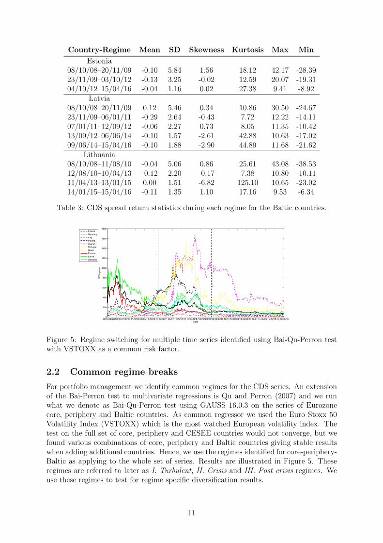
Table 3: CDS spread return statistics during each regime for the Baltic countries.
08/10/08 28/02/09 21/07/09 11/12/09 03/05/10 23/09/10 13/02/11 06/07/11 26/11/11 17/04/12 07/09/12 28/01/13 20/06/13 10/11/13 02/04/14 23/08/14 13/01/15 05/06/15 26/10/15 18/03/160
200
400
600
800
1000
1200
1400
1600
1800
Date
CD
S s
pre
ad
France
Germany
Italy
Ireland
Cyprus
Portugal
Spain
Estonia
Latvia
Lithuania
Figure 5: Regime switching for multiple time series identified using Bai-Qu-Perron testwith VSTOXX as a common risk factor.
2.2 Common regime breaks
For portfolio management we identify common regimes for the CDS series. An extensionof the Bai-Perron test to multivariate regressions is Qu and Perron (2007) and we runwhat we denote as Bai-Qu-Perron test using GAUSS 16.0.3 on the series of Eurozonecore, periphery and Baltic countries. As common regressor we used the Euro Stoxx 50Volatility Index (VSTOXX) which is the most watched European volatility index. Thetest on the full set of core, periphery and CESEE countries would not converge, but wefound various combinations of core, periphery and Baltic countries giving stable resultswhen adding additional countries. Hence, we use the regimes identified for core-periphery-Baltic as applying to the whole set of series. Results are illustrated in Figure 5. Theseregimes are referred to later as I. Turbulent, II. Crisis and III. Post crisis regimes. Weuse these regimes to test for regime specific diversification results.
11

3 The CVaR portfolio optimization models
We consider now the model for building a diversified portfolio of credit default swappositions using CVaR portfolio optimization, which is well suited for the skewed andfat-tailed returns of CDS. CVaR optimization has its origins in the work of Rockafellarand Uryasev (2000) and its properties are well understood, see, e.g., Zenios (2007) fordiscussion and references. The CVaR optimization models we develop are single-period.We measure returns during the risk horizon by spread changes, but do not account forcollected premia or payments in the case of default. This is a reasonable approximation forshort horizons or when dealing with sovereigns without potential default (e.g, Germanyor the US). In the conclusions we discuss extensions of the models beyond these limitingassumptions.
The expected value of the α-tail2 of the distribution of portfolio loss X, CVaRα(X),and its minimization formula are given in the following theorem:
Theorem 3.1 Fundamental minimization formula (Rockafellar and Uryasev, 2002)As a function of γ ∈ R, the auxiliary function
Fα(X, γ) = γ +1
1− αE{[X − γ]+},
where α ∈ (0, 1] is the confidence level and [t]+ = max{0, t}, is finite and convex, with
CVaRα(X) = minγ∈R
Fα(X, γ).
Consider an investor operating in a market with n risky assets with rates of returndenoted by random vector ξ. For an investment vector x ∈ Rn of notional proportionalallocations to the risky assets, the loss function is given by f(x, ξ) = −x>ξ. Whendealing with portfolio optimization, loss is a function of the portfolio x and we write theauxiliary function and CVaR as functions of x. According to Theorem 3.1 the conditionalvalue-at-risk of the loss function is the solution of
CVaRα(x) = minγ∈R
Fα(x, γ), (1)
where
Fα(x, γ) = γ +1
1− αE{[f(x, ξ)− γ]+}.
Hence, models for selecting a portfolio with minimum CVaR and a target expectedreturn constraint can be posed as:
minγ∈R,x∈X
Fα(x, γ) (2)
s.t. µ>x ≥ µ.
X is the constraint set on the investment variables which specifies feasible portfolios, µ isa vector of mean returns of risky assets, and µ ∈ R is the target expected return.
2α ∈ (0, 1] and all numerical experiments in this paper are carried out for α = 0.95.
12

From historical data we generate an S×n matrix R of return scenarios for the n riskyassets —see Steps 0 to 3 in Section 5— and µ is the vector of mean returns of R. From(2) we formulate CVaR optimization models for three investment strategies:
1. Long exposures (L). This is for using CDS as they were originally intended to hedgecredit risk, but never, so far, employed in a portfolio context.
2. Uncovered long and short exposures (LS). This is the strategy followed by specu-lators that seek to exploit credit risk opportunities from deterioration (using longpositions) or improvements (using short positions) of a sovereign’s rating.
3. Covered long and short exposures (NZ). This is the strategy of dealers that bothbuy and sell CDS but do not wish to have uncovered exposures. This could be a“net zero” position with no net cash outflows.
The notion of covered and uncovered position differs depending on the context. Typi-cally a short CDS position is covered if the investor has borrowed the share or has enteredinto an agreement to borrow the share, or has an arrangement with a third party thatguarantees that the share can be made available. In our work we consider a positioncovered if, on the aggregate, there are as many long positions as there are short.
3.1 Long exposures
The constraint set on the investment variables stipulates that all variables are non-negative (i.e., no short sales allowed) with a proportionality condition that nominal assetallocations add up to an initial endowment of 1, i.e.,
XL = {x ∈ Rn | x ≥ 0,n∑i=1
xi = 1}. (3)
The CVaR portfolio optimization model is given by
minx∈XL, u∈RS , γ∈R
γ +1
S(1− α)e>u (4)
s.t.
−Rx− u− eγ ≤ 0
µ>x ≥ µ
u ≥ 0,
where e is a vector of all 1.
3.2 Uncovered long and short exposures
We introduce non-negative variables x+ and x− to represent long and short positions,respectively. We assume a starting wealth of 1 unit to be invested in long positions,but the long positions can be augmented from capital raised by short sales. We set an(arbitrary) limit that no single short position can be higher than our original endowment,but overall there is no guarantee that the aggregate short positions will not be significantlyhigher that the original endowment. The difference between the original endowment and
13

the aggregate short position (if negative) is a proxy for the margin that the investor needsto put down in order to sell CDS protection.
The constraint set on the investment variables is given by
XLS = {x ∈ Rn | x = x+ − x−, 0 ≤ x+, x− ≤ 1,n∑i=1
(x+i − x−i ) = 1}, (5)
and the CVaR portfolio optimization model by
minx+,x−∈Rn, u∈RS , γ∈R
γ +1
S(1− α)e>u (6)
s.t.
−Rx+ +Rx− − u− eγ ≤ 0
µ>x+ − µ>x− ≥ µn∑i=1
(x+i − x−i ) = 1
0 ≤ x+, x− ≤ 1
u ≥ 0.
3.3 Covered long and short exposures
We impose now a constraint that total short position is equal to total long position. Thisis a net zero position with no net cash outflow required, with the endowment of 1 unitconsidered as collateral. The constraint set on the investment variables is given by
XNZ = {x ∈ Rn | x = x+ − x−, 0 ≤ x+, x− ≤ 1,n∑i=1
x+i = 1,n∑i=1
x−i = 1}, (7)
and the CVaR portfolio optimization formulation by
minx+,x−∈Rn, u∈RS , γ∈R
γ +1
S(1− α)e>u (8)
s.t.
−Rx+ +Rx− − u− eγ ≤ 0
µ>x+ − µ>x− ≥ µn∑i=1
x+i = 1,n∑i=1
x−i = 1
0 ≤ x+, x− ≤ 1
u ≥ 0.
All models can be easily modified to incorporate linearly proportional transactioncosts, (Zenios, 2007, pp. 80–81), and all numerical experiments are carried out withtransaction cost 0.5%.
14
4 Portfolio diversification
The S scenarios of returns are taken to be all possible realization of historical dataobserved during the time period of interest. To make our empirical testing consistentwith our modeling setup, Greece was excluded form the portfolio experiments since itdefaulted during the testing period. We develop efficient frontiers for the whole timeperiod and for each one of the three regimes separately. Frontiers are developed for thethree investment strategies we modeled, L, LS, and NZ.
4.1 Diversification pays
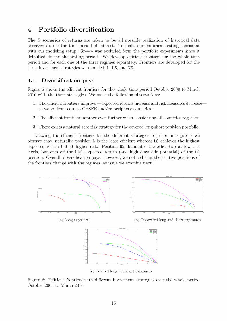
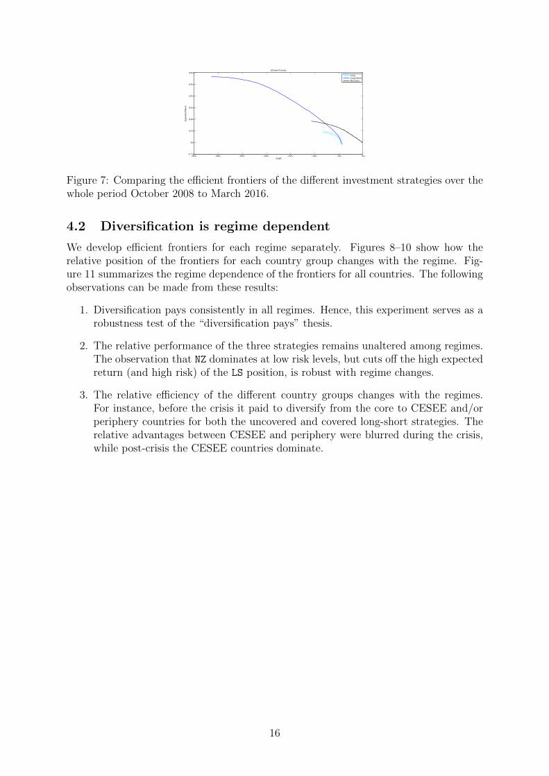
Figure 6 shows the efficient frontiers for the whole time period October 2008 to March2016 with the three strategies. We make the following observations:
1. The efficient frontiers improve —expected returns increase and risk measures decrease—as we go from core to CESEE and/or periphery countries.
2. The efficient frontiers improve even further when considering all countries together.
3. There exists a natural zero risk strategy for the covered long-short position portfolio.
Drawing the efficient frontiers for the different strategies together in Figure 7 weobserve that, naturally, position L is the least efficient whereas LS achieves the highestexpected return but at higher risk. Position NZ dominates the other two at low risklevels, but cuts off the high expected return (and high downside potential) of the LS
position. Overall, diversification pays. However, we noticed that the relative positions ofthe frontiers change with the regimes, as issue we examine next.
−12% −11% −10% −9% −8% −7% −6% −5% −4%−0.05%
0%
0.05%
0.1%
CVaR
Expecte
d R
etu
rn
Efficient Frontier
Core
Periphery
CESEE
All
(a) Long exposures
−35% −30% −25% −20% −15% −10% −5% 0%−0.1%
0%
0.1%
0.2%
0.3%
0.4%
0.5%
0.6%
CVaR
Expecte
d R
etu
rn
Efficient Frontier
Core
Periphery
CESEE
All
(b) Uncovered long and short exposures
−14% −12% −10% −8% −6% −4% −2% 0% 0%
0.02%
0.04%
0.06%
0.08%
0.1%
0.12%
0.14%
0.16%
0.18%
0.2%
CVaR
Expecte
d R
etu
rn
Efficient Frontier
Core
Periphery
CESEE
All
(c) Covered long and short exposures
Figure 6: Efficient frontiers with different investment strategies over the whole periodOctober 2008 to March 2016.
15
−35% −30% −25% −20% −15% −10% −5% 0%−0.1%
0%
0.1%
0.2%
0.3%
0.4%
0.5%
0.6%
CVaR
Expecte
d R
etu
rn
Efficient Frontier
Long
Long−Short
Net−Zero
Figure 7: Comparing the efficient frontiers of the different investment strategies over thewhole period October 2008 to March 2016.
4.2 Diversification is regime dependent
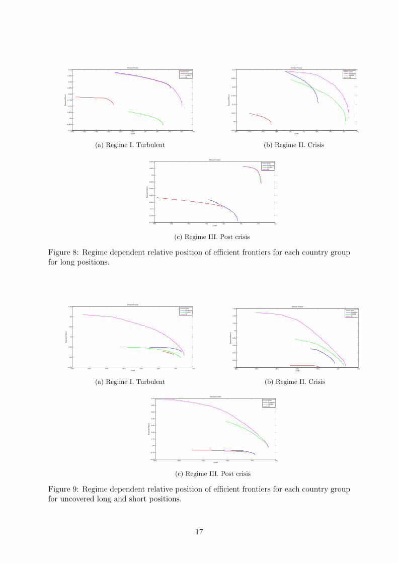
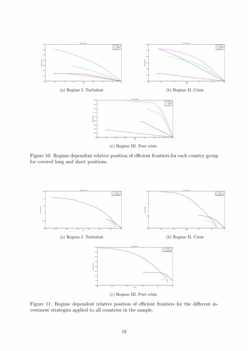
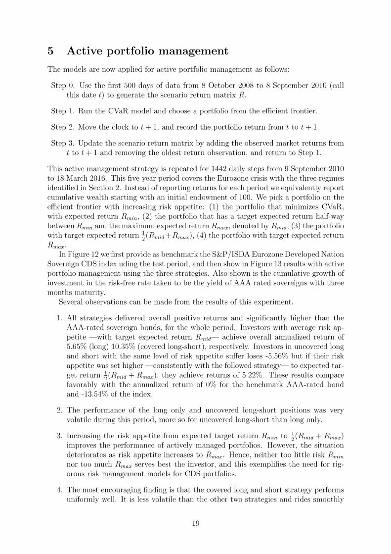
We develop efficient frontiers for each regime separately. Figures 8–10 show how therelative position of the frontiers for each country group changes with the regime. Fig-ure 11 summarizes the regime dependence of the frontiers for all countries. The followingobservations can be made from these results:
1. Diversification pays consistently in all regimes. Hence, this experiment serves as arobustness test of the “diversification pays” thesis.
2. The relative performance of the three strategies remains unaltered among regimes.The observation that NZ dominates at low risk levels, but cuts off the high expectedreturn (and high risk) of the LS position, is robust with regime changes.
3. The relative efficiency of the different country groups changes with the regimes.For instance, before the crisis it paid to diversify from the core to CESEE and/orperiphery countries for both the uncovered and covered long-short strategies. Therelative advantages between CESEE and periphery were blurred during the crisis,while post-crisis the CESEE countries dominate.
16
−15% −14% −13% −12% −11% −10% −9% −8% −7% −6% −5% −0.1%
−0.05%
0%
0.05%
0.1%
0.15%
0.2%
0.25%
0.3%
0.35%
0.4%
CVaR
Expecte
d R
etu
rn
Efficient Frontier
Core
Periphery
CESEE
All
(a) Regime I. Turbulent
−12% −11% −10% −9% −8% −7% −6% −5% −4% −3%−0.05%
0%
0.05%
0.1%
0.15%
0.2%
0.25%
0.3%
CVaR
Expecte
d R
etu
rn
Efficient Frontier
Core
Periphery
CESEE
All
(b) Regime II. Crisis
−14% −12% −10% −8% −6% −4% −2% 0%−0.14%
−0.12%
−0.1%
−0.08%
−0.06%
−0.04%
−0.02%
0%
0.02%
0.04%
CVaR
Expecte
d R
etu
rn
Efficient Frontier
Core
Periphery
CESEE
All
(c) Regime III. Post crisis
Figure 8: Regime dependent relative position of efficient frontiers for each country groupfor long positions.
−70% −60% −50% −40% −30% −20% −10% 0%−0.5%
0%
0.5%
1%
1.5%
2%
2.5%
CVaR
Expecte
d R
etu
rn
Efficient Frontier
Core
Periphery
CESEE
All
(a) Regime I. Turbulent
−30% −25% −20% −15% −10% −5% 0%0%
0.2%
0.4%
0.6%
0.8%
1%
1.2%
1.4%
1.6%
CVaR
Expecte
d R
etu
rn
Efficient Frontier
Core
Periphery
CESEE
All
(b) Regime II. Crisis
−25% −20% −15% −10% −5% 0%−0.2%
−0.1%
0%
0.1%
0.2%
0.3%
0.4%
0.5%
0.6%
0.7%
CVaR
Expecte
d R
etu
rn
Efficient Frontier
Core
Periphery
CESEE
All
(c) Regime III. Post crisis
Figure 9: Regime dependent relative position of efficient frontiers for each country groupfor uncovered long and short positions.
17
−16% −14% −12% −10% −8% −6% −4% −2% 0% 0%
0.1%
0.2%
0.3%
0.4%
0.5%
0.6%
0.7%
CVaR
Expecte
d R
etu
rn
Efficient Frontier
Core
Periphery
CESEE
All
(a) Regime I. Turbulent
−12% −10% −8% −6% −4% −2% 0% 0%
0.1%
0.2%
0.3%
0.4%
0.5%
0.6%
CVaR
Expecte
d R
etu
rn
Efficient Frontier
Core
Periphery
CESEE
All
(b) Regime II. Crisis
−16% −14% −12% −10% −8% −6% −4% −2% 0% 0%
0.02%
0.04%
0.06%
0.08%
0.1%
0.12%
0.14%
0.16%
0.18%
CVaR
Expecte
d R
etu
rn
Efficient Frontier
Core
Periphery
CESEE
All
(c) Regime III. Post crisis
Figure 10: Regime dependent relative position of efficient frontiers for each country groupfor covered long and short positions.
−70% −60% −50% −40% −30% −20% −10% 0%0%
0.05%
1%
1.5%
2%
2.5%
CVaR
Expecte
d R
etu
rn
Efficient Frontier
Long
Long−Short
Net−Zero
(a) Regime I. Turbulent
−3% −25% −20% −15% −10% −5% 0% 0%
0.5%
1%
1.5%
CVaR
Expecte
d R
etu
rn
Efficient Frontier
Long
Long−Short
Net−Zero
(b) Regime II. Crisis
−25% −20% −15% −10% −5% 0%−0.1%
0%
0.1%
0.2%
0.3%
0.4%
0.5%
0.6%
0.7%
CVaR
Expecte
d R
etu
rn
Efficient Frontier
Long
Long−Short
Net−Zero
(c) Regime III. Post crisis
Figure 11: Regime dependent relative position of efficient frontiers for the different in-vestment strategies applied to all countries in the sample.
18
5 Active portfolio management
The models are now applied for active portfolio management as follows:
Step 0. Use the first 500 days of data from 8 October 2008 to 8 September 2010 (callthis date t) to generate the scenario return matrix R.
Step 1. Run the CVaR model and choose a portfolio from the efficient frontier.
Step 2. Move the clock to t+ 1, and record the portfolio return from t to t+ 1.
Step 3. Update the scenario return matrix by adding the observed market returns fromt to t+ 1 and removing the oldest return observation, and return to Step 1.
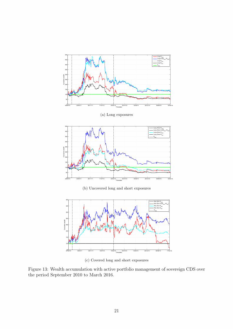
This active management strategy is repeated for 1442 daily steps from 9 September 2010to 18 March 2016. This five-year period covers the Eurozone crisis with the three regimesidentified in Section 2. Instead of reporting returns for each period we equivalently reportcumulative wealth starting with an initial endowment of 100. We pick a portfolio on theefficient frontier with increasing risk appetite: (1) the portfolio that minimizes CVaR,with expected return Rmin, (2) the portfolio that has a target expected return half-waybetween Rmin and the maximum expected return Rmax, denoted by Rmid, (3) the portfoliowith target expected return 1
2(Rmid+Rmax), (4) the portfolio with target expected return
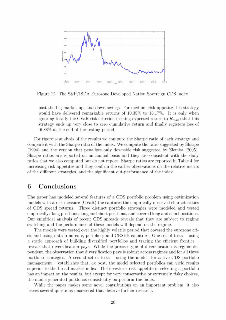
Rmax.In Figure 12 we first provide as benchmark the S&P/ISDA Eurozone Developed Nation
Sovereign CDS index uding the test period, and then show in Figure 13 results with activeportfolio management using the three strategies. Also shown is the cumulative growth ofinvestment in the risk-free rate taken to be the yield of AAA rated sovereigns with threemonths maturity.
Several observations can be made from the results of this experiment.
1. All strategies delivered overall positive returns and significantly higher than theAAA-rated sovereign bonds, for the whole period. Investors with average risk ap-petite —with target expected return Rmid— achieve overall annualized return of5.65% (long) 10.35% (covered long-short), respectively. Investors in uncovered longand short with the same level of risk appetite suffer loses -5.56% but if their riskappetite was set higher —consistently with the followed strategy— to expected tar-get return 1
2(Rmid + Rmax), they achieve returns of 5.22%. These results compare
favorably with the annualized return of 0% for the benchmark AAA-rated bondand -13.54% of the index.
2. The performance of the long only and uncovered long-short positions was veryvolatile during this period, more so for uncovered long-short than long only.
3. Increasing the risk appetite from expected target return Rmin to 12(Rmid + Rmax)
improves the performance of actively managed portfolios. However, the situationdeteriorates as risk appetite increases to Rmax. Hence, neither too little risk Rmin
nor too much Rmax serves best the investor, and this exemplifies the need for rig-orous risk management models for CDS portfolios.
4. The most encouraging finding is that the covered long and short strategy performsuniformly well. It is less volatile than the other two strategies and rides smoothly
19
08/09/10 20/04/11 30/11/11 11/07/12 20/02/13 03/10/13 15/05/14 25/12/14 06/08/15 18/03/160
50
100
150
200
250
300
350
Date
S&
P E
uro
CD
S (
%)
Figure 12: The S&P/ISDA Eurozone Developed Nation Sovereign CDS index.
past the big market up- and down-swings. For medium risk appetite this strategywould have delivered remarkable returns of 10.35% to 18.17%. It is only whenignoring totally the CVaR risk criterion (setting expected return to Rmax) that thisstrategy ends up very close to zero cumulative return and finally registers loss of-6.88% at the end of the testing period.
For rigorous analysis of the results we compute the Sharpe ratio of each strategy andcompare it with the Sharpe ratio of the index. We compute the ratio suggested by Sharpe(1994) and the version that penalizes only downside risk suggested by Ziemba (2005).Sharpe ratios are reported on an annual basis and they are consistent with the dailyratios that we also computed but do not report. Sharpe ratios are reported in Table 4 forincreasing risk appetites and they confirm the earlier observations on the relative meritsof the different strategies, and the significant out-performance of the index.
6 Conclusions
The paper has modeled several features of a CDS portfolio problem using optimizationmodels with a risk measure (CVaR) the captures the empirically observed characteristicsof CDS spread returns. Three distinct portfolio strategies were modeled and testedempirically: long positions, long and short positions, and covered long and short positions.Our empirical analysis of recent CDS spreads reveals that they are subject to regimeswitching and the performance of these models will depend on the regime.
The models were tested over the highly volatile period that covered the eurozone cri-sis and using data from core, periphery and CESEE countries. One set of tests —usinga static approach of building diversified portfolios and tracing the efficient frontier—reveals that diversification pays. While the precise type of diversification is regime de-pendent, the observation that diversification pays is robust across regimes and for all threeportfolio strategies. A second set of tests —using the models for active CDS portfoliomanagement— establishes that, ex post, the model selected portfolios can yield resultssuperior to the broad market index. The investor’s risk appetite in selecting a portfoliohas an impact on the results, but except for very conservative or extremely risky choices,the model generated portfolios consistently outperform the index.
While the paper makes some novel contributions on an important problem, it alsoleaves several questions unaswered that deserve further research.
20
08/09/10 20/04/11 30/11/11 11/07/12 20/02/13 03/10/13 15/05/14 25/12/14 06/08/15 18/03/160
50
100
150
200
250
300
350
400
450
500
Time(date)
Cum
ula
tive w
ealth
Long Rmax
Long 0.5(Rmax
+Rmid
)
Long Rmid
Long Rmin
Rfree
(a) Long exposures
08/09/10 20/04/11 30/11/11 11/07/12 20/02/13 03/10/13 15/05/14 25/12/14 06/08/15 18/03/160
50
100
150
200
250
300
350
400
450
500
Time(date)
Cum
ula
tive w
ealth
Long−Short Rmax
Long−Short 0.5(Rmax
+Rmid
)
Long−Short Rmid
Long−Short Rmin
Rfree
(b) Uncovered long and short exposures
07/09/10 19/04/11 29/11/11 10/07/12 19/02/13 02/10/13 14/05/14 24/12/14 05/08/15 17/03/1650
100
150
200
250
300
350
400
450
Time(date)
Cum
ula
tive w
ealth
Net−Zero Rmax
Net−Zero 0.5(Rmax
+Rmid
)
Net−Zero Rmid
Net−Zero Rmin
Rfree
(c) Covered long and short exposures
Figure 13: Wealth accumulation with active portfolio management of sovereign CDS overthe period September 2010 to March 2016.
21
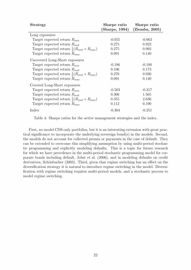
Strategy Sharpe ratio Sharpe ratio(Sharpe, 1994) (Ziemba, 2005)
Long exposuresTarget expected return Rmin -0.055 -0.063Target expected return Rmid 0.275 0.922Target expected return 1
2(Rmid +Rmax) 0.275 0.992
Target expected return Rmax 0.091 0.140
Uncovered Long-Short exposuresTarget expected return Rmin -0.186 -0.180Target expected return Rmid 0.106 0.173Target expected return 1
2(Rmid +Rmax) 0.276 0.930
Target expected return Rmax 0.091 0.140
Covered Long-Short exposuresTarget expected return Rmin -0.503 -0.317Target expected return Rmid 0.306 1.565Target expected return 1
2(Rmid +Rmax) 0.355 2.636
Target expected return Rmax 0.112 0.190
Index -0.304 -0.251
Table 4: Sharpe ratios for the active management strategies and the index.
First, we model CDS-only portfolios, but it is an interesting extension with great prac-tical significance to incorporate the underlying sovereign bond(s) in the models. Second,the models do not account for collected premia or payments in the case of default. Theycan be extended to overcome this simplifying assumption by using multi-period stochas-tic programming and explicitly modeling defaults. This is a topic for future researchfor which we have precedence in the multi-period stochastic programming model for cor-porate bonds including default, Jobst et al. (2006), and in modeling defaults on creditderivatives, Schonbucher (2003). Third, given that regime switching has an effect on thediversification strategy it is natural to introduce regime switching in the model. Diversi-fication with regime switching requires multi-period models, and a stochastic process tomodel regime switching.
22
References
P. Augustin, M.G. Subrahmanyam, D. Y. Tang, and S. Q. Wang. Credit default swaps:a survey. Foundations and Trends in Finance, 9(1–2):1–196, 2014.
P. Augustin, M.G. Subrahmanyam, D. Y. Tang, and S. Q. Wang. Credit default swaps:Past, present, and future. Annual Review of Financial Economics, (in print), 2016.
J. Bai and P. Perron. Evaluating and testing linear models with multiple structuralchanges. Eonometrica, 66(1):47–78, 1998.
S. Criado, L. Degabriel, M. Lewandowska, S. Linden, and P. Ritter. Sovereign CDS report.Official report DG COMP, DG ECFIN and DG MARKT, European Commission,Brussels, 2010.
European Union. Regulation (EU) of the European Parliament and the Council on shortselling and certain aspects of credit default swaps. Regulation EU 236/2012, OfficalJournal of the European Union, 2012.
F. Fabozzi, R. Giacometti, and N. Tsuchida. Factor decomposition of the eurozonesovereign CDS spreads. Journal of International Money and Finance, (in print), 2016.
IMF. A New Look at the Role of Sovereign Credit Default Swaps, volume Global FinancialStability Report, chapter 2, pages 57–92. International Monetary Fund, Washington,DC., April 2013.
N. Jobst, G. Mitra, and S.A. Zenios. Integrating market and credit risk: A simulationand optimization perspective. Journal of Banking and Finance, 30(2):645–667, 2006.
F. Packer and C. Suthiphongchai. Sovereign credit default swaps. BIS Quarterly Review,pages 79–88, December 2003.
Z. Qu and P. Perron. Estimating and Testing Structural Changes in Multivariate Re-gressions. Econometrica, 75(March):459–502, March 2007.
R. Rockafellar and S. Uryasev. Conditional Value-at-Risk for general loss distributions.Journal of Banking and Finance, 26:1443–1471, 2002.
R.T. Rockafellar and S. Uryasev. Optimization of conditional Value–at–Risk. Journal ofRisk, 2(3):21–41, 2000.
P. Schonbucher. Credit Derivatives Pricing Models: Models, Pricing and Implementation.Wiley Finance, New York, NY, 2003.
W.F. Sharpe. The Sharpe ratio. The Journal of Portfolio Management, pages 49–58, Fall1994.
R. Stulz. Credit default swaps and the credit crisis. Journal of Economic Perspectives,24(1):73–92, 2010.
S.A. Zenios. Practical Financial Optimization. Decision making for financial engineers.Blackwell, Malden, MA, 2007.
W. T. Ziemba. The symmetric downside risk Sharpe ratio. Journal of Portfolio Manage-ment, 32(1):108–122, 2005.
23