sources of macroeconomic fluctuations: a regime-switching ... · sources of macroeconomic...
TRANSCRIPT

FEDERAL RESERVE BANK OF SAN FRANCISCO
WORKING PAPER SERIES
Working Paper 2009-01 http://www.frbsf.org/publications/economics/papers/2009/wp09-01bk.pdf
The views in this paper are solely the responsibility of the authors and should not be interpreted as reflecting the views of the Federal Reserve Bank of San Francisco or the Board of Governors of the Federal Reserve System.
Sources of Macroeconomic Fluctuations: A
Regime-Switching DSGE Approach
Zheng Liu Federal Reserve Bank of San Francisco
Daniel F. Waggoner
Federal Reserve Bank of Atlanta
Tao Zha Federal Reserve Bank of Atlanta and Emory University
April 2010
SOURCES OF MACROECONOMIC FLUCTUATIONS: AREGIME-SWITCHING DSGE APPROACH
ZHENG LIU, DANIEL F. WAGGONER, AND TAO ZHA
Abstract. We examine the sources of macroeconomic economic fluctuations by es-timating a variety of medium-scale DSGE models within a unified framework thatincorporates regime switching both in shock variances and in the inflation target. Ourgeneral framework includes a number of different model features studied in the liter-ature. We propose an efficient methodology for estimating regime-switching DSGEmodels. The model that best fits the U.S. time-series data is the one with synchro-nized shifts in shock variances across two regimes and the fit does not rely on strongnominal rigidities. We find little evidence of changes in the inflation target. Weidentify three types of shocks that account for most of macroeconomic fluctuations:shocks to total factor productivity, wage markup, and the capital depreciation rate.
I. Introduction
We examine the sources of macroeconomic fluctuations by estimating a number ofregime-switching models using modern Bayesian techniques in a unified dynamic sto-chastic general equilibrium (DSGE) framework. The standard approach to analyzingbusiness-cycle fluctuations is the use of constant-parameter medium-scale DSGE mod-els (Altig, Christiano, Eichenbaum, and Linde, 2004; Christiano, Eichenbaum, andEvans, 2005; Levin, Onatski, Williams, and Williams, 2006; Smets and Wouters, 2007;Del Negro, Schorfheide, Smets, and Wouters, 2007). In this paper we generalize the
Date: April 4, 2010.Key words and phrases. Systematic analysis, regime switching, depreciation shock, efficient esti-
mation methods.JEL classification: C11, C51, E32, E42, E52.We thank Craig Burnside, Larry Christiano, Tim Cogley, Chris Erceg, Marco Del Negro, Wouter
Den Haan, Martin Ellison, Jesus Fernandez-Villaverde, Jordi Gali, Marc Giannoni, Michael Golosov,Pat Higgins, Alejandro Justiniano, Soyoung Kim, Junior Maih, Christian Matthes, Ulrich Müeller,Andy Levin, Lee Ohanian, Pietro F. Peretto, Giorgio Primiceri, Frank Schorfheide, Chris Sims, HaraldUhlig, and seminar participants at the Bank of Korea, NBER summer institute, UC Berkeley, SED,and Duke University for helpful discussions and comments. Eric Wang provided valuable assistancein grid computing. The views expressed herein are those of the authors and do not necessarily reflectthe views of the Federal Reserve Banks of Atlanta and San Francisco or the Federal Reserve System.
1

SOURCES OF MACROECONOMIC FLUCTUATIONS 2
standard approach by allowing time variations in shock variances and in the centralbank’s inflation target according to Markov-switching processes. These time variationsappear to be present in the U.S. macroeconomic time series. An important question ishow significant the time variations are when we fit the data to relatively large DSGEmodels with rich dynamic structures and shock processes that are economically inter-pretable. If the answer is positive, the next equation is in what dimension the timevariations matter. To answer these questions, we estimate a number of alternativemodels nested in this general framework using the Bayesian method and we comparethe fit of these models to the time series data in the postwar U.S. economy. The best-fit model is then used to identify shocks that are important in driving macroeconomicfluctuations.
Our approach yields several new results. We find strong empirical evidence in favorof the DSGE model with two regimes in shock variances, where regime shifts in thevariances are synchronized. The models with constant parameters (i.e., no regimeshifts), with independent regime shifts in shock variances, or with more than tworegimes do not fit to the data as well. In our preferred model (i.e., the best-fit model)with two synchronized shock regimes, the high-volatility regime was frequently observedin the period from the early 1970s through the mid-1980s, while the low-volatilityregime prevailed in most of the period from the mid-1980s through 2007. This findingis broadly consistent with the well-known fact that the U.S. economy experienced ageneral reduction in macroeconomic volatilities during the latter sample period (Stockand Watson, 2003).
The fit of our preferred regime-switching DSGE model does not reply on strongnominal rigidities. In particular, our estimates imply that the durations of the priceand nominal wage contracts last no more than 2 quarters of a year—much shorter thanthose reported in the constant-parameter DSGE models in previous studies (Smets andWouters, 2007). This finding highlights the sensitivity of the estimates of some keystructural parameters obtained in models with no regime switching to specifications ofthe shock processes. When we allow the shock variances to switch regimes, the modelrelies less on nominal rigidities to fit to the data.
Neither does the fit of our preferred model reply on regime shifts in the inflation tar-get. Allowing the inflation target to shift between two regimes—either synchronizedwith or independent of the shock regime switching—does not improve the model’s mar-ginal data density. This finding is robust to a variety of model specifications and it isconsistent with the conclusion from other works about changes in monetary policy in

SOURCES OF MACROECONOMIC FLUCTUATIONS 3
general (Stock and Watson, 2003; Canova and Gambetti, 2004; Cogley and Sargent,2005; Primiceri, 2005; Sims and Zha, 2006; Justiniano and Primiceri, 2008). We focuson studying changes in the inflation target instead of changes in monetary policy’sresponse to inflation for both conceptual and computational reasons. When agentstake into account changes in monetary policy’s response to inflation in forming theirexpectations, a solution method to the model is nonstandard (Liu, Waggoner, and Zha,2009). Indeed, it would be computationally infeasible for us to estimate a large set ofDSGE models like what we do in the current paper since the solution would require aniterative algorithm that can be time-consuming in Monte Carlo simulations. Further-more, indeterminacy is more prevalent in this kind of regime-switching model than inthe standard DSGE model (Farmer, Waggoner, and Zha, 2009). For these reasons, wefollow Schorfheide (2005) and Ireland (2005) and focus on examining changes in theinflation target to give the model the best chance to detect changes in monetary policy.Although we can apply the standard method to solving our regime-switching DSGEmodels (as shown in Section V), we have nonetheless pushed the limits of our compu-tational and analytical capacity because of a large set of regime-switching models wehave estimated.
In the best-fit model, we identify three types of shocks that are important for macroe-conomic fluctuations. These are a shock to the growth rate of the total factor produc-tivity (TFP), a shock to wage markups, and a shock to the capital depreciation rate.Taken together, these three shocks account for about 70−80% of the variances of aggre-gate output, investment, and inflation at business cycle frequencies. Other shocks suchas monetary policy shocks, investment-specific technology shocks, and price markupshocks are not as important. The TFP shocks and the wage markup shocks should befamiliar to a student of the DSGE literature, but the capital depreciation shock is new.We provide some economic interpretations of the depreciation shock in Section VII.3.
In what follows, we briefly discuss our contributions in relation to the literaturein Section II. We then present, in Section III, the general regime-switching DSGEframework. In Section IV, we present the system of equilibrium conditions and discussour solution methods. In Section V, we describe the data and our empirical approach.As a methodological contribution, we propose an efficient methodology for estimatingregime-switching DSGE models; we summarize and discuss several modern methodsfor obtaining accurate estimates of marginal data densities for relatively large DSGEmodels. In Section VI, we compare the fit of a number of models nested by our generalDSGE framework, identify the best-fit model, and report posterior estimates of the
SOURCES OF MACROECONOMIC FLUCTUATIONS 4
parameters in this model. In Section VII, we discuss the economic implications ofour estimates in the best-fit model and identify the key sources of shocks that drivemacroeconomic fluctuations. We conclude in Section VIII.
II. Related literature
The debate in the literature on the sources of macroeconomic fluctuations givesemphasis to whether shifts in monetary policy are the main sources of macroeconomicvolatilities (Clarida, Galí, and Gertler, 2000; Lubik and Schorfheide, 2004; Stock andWatson, 2003; Sims and Zha, 2006; Bianchi, 2008; Gambetti, Pappa, and Canova,2008) or whether shocks in investment-specific technology are more important thanother shocks in driving macroeconomic fluctuations (Fisher, 2006; Smets and Wouters,2007; Justiniano and Primiceri, 2008). Much of the disagreement stems from the use ofdifferent frameworks and different empirical methods. Part of the literature focuses onreduced-form econometric models, part of it on small-scale DSGE models, and part of iton medium-scale DSGE models. Some models assume homogeneity in shock variances;others assume that shock variances are time-varying. Some models are estimated withdifferent subsamples to reflect shifts in policy or in shock variances; other models areestimated with the entire sample. Given these differences in the model frameworkand in the empirical approach, it is difficult to draw a firm conclusion about thesources of macroeconomic fluctuations. The goal of the current paper is to providea systematic examination of the sources of macroeconomic fluctuations in one unifiedDSGE framework that allows for regime shifts in shock variances and in monetarypolicy.
Our approach differs from that employed in the literature in several aspects. First,we aim at fully characterizing the uncertainty across different models by examiningdifferent versions of the DSGE model for robust analysis to substantiate our conclusion.Although estimating a large set of models has not been performed in the literature, wethink it is necessary to examine the robustness of a conclusion like ours about potentialsources of macroeconomic fluctuations.
Second, our approach does not require splitting the sample to examine changes inmonetary policy, although it nests sampling-splitting as a special case. Unlike Simsand Zha (2006) where the number of VAR parameters is relatively large and the in-flation target is implicit, our way of modeling policy changes takes the inflation targetexplicitly and gives a tightly parameterized model that has the best chance to detectthe importance of policy changes, if it exists, in generating business-cycle fluctuations.
SOURCES OF MACROECONOMIC FLUCTUATIONS 5
Third and methodologically, for fairly large DSGE models, especially for regime-switching DSGE models, the posterior distribution tends to be very non-Gaussian,making it very challenging to search for the global peak. We improve on earlier workssuch as Cogley and Sargent (2005) and Justiniano and Primiceri (2006) by obtaining theestimate of parameters at the posterior mode for each model. We show that economicimplications can be seriously distorted if the estimates are based on a lower posteriorpeak.
Fourth, there is a strand of literature that emphasizes changes in the inflation targetas a representation of important shifts in the conduct of U.S. monetary policy (for ex-ample, Favero and Rovelli (2003); Erceg and Levin (2003); Schorfheide (2005); Ireland(2005). Unlike the earlier works, we study a variety of fairly large DSGE models toavoid potential mis-specifications.
Finally, we use three new methods for computing marginal data densities in modelcomparison. Since these methods are based on different statistical foundations, it isessential that all these methods give a numerically similar result to ensure that theestimate of a marginal data density is unbiased and accurate (Sims, Waggoner, andZha, 2008).
III. The Model
The model economy is populated by a continuum of households, each endowed witha unit of differentiated labor skill indexed by i ∈ [0, 1]; and a continuum of firms, eachproducing a differentiated good indexed by j ∈ [0, 1]. The monetary authority followsa feedback interest rate rule, under which the nominal interest rate is set to respond toits own lag and deviations of inflation and output from their targets. The policy regimest represented by the time-varying inflation target switches between a finite number ofregimes contained in the set S, with the Markov transition probabilities summarizedby the matrix Q = [qij], where qij = Prob(st+1 = i|st = j) for i, j ∈ S. The economyis buffeted by several sources of shocks. The variance of each shock switches betweena finite number of regimes denoted by s∗t ∈ S∗ with the transition matrix Q∗ = [q∗ij].
III.1. The aggregation sector. The aggregation sector produces a composite laborskill denoted by Lt to be used in the production of each type of intermediate goods and acomposite final good denoted by Yt to be consumed by each household. The productionof the composite skill requires a continuum of differentiated labor skills {Lt(i)}i∈[0,1]
as inputs, and the production of the composite final good requires a continuum ofdifferentiated intermediate goods {Yt(j)}j∈[0,1] as inputs. The aggregation technologies
SOURCES OF MACROECONOMIC FLUCTUATIONS 6
are given by
Lt =
[∫ 1
0
Lt(i)1
µwt di
]µwt
, Yt =
[∫ 1
0
Yt(j)1
µpt dj
]µpt
, (1)
where µwt and µpt determine the elasticity of substitution between the skills and be-tween the goods, respectively. Following Smets and Wouters (2007), we assume that
ln µwt = (1 − ρw) ln µw + ρw ln µw,t−1 + σwtεwt − ϕwσw,t−1εw,t−1 (2)
and that
ln µpt = (1 − ρp) ln µp + ρp ln µp,t−1 + σptεpt − ϕpσp,t−1εp,t−1, (3)
where, for j ∈ {w, p}, ρj ∈ (−1, 1) is the AR(1) coefficient, ϕj is the MA(1) coefficient,σjt ≡ σj(s
∗t ) is the regime-switching standard deviation, and εjt is an i.i.d. white noise
process with a zero mean and a unit variance. We interpret µwt and µpt as the wagemarkup and price markup shocks.
The representative firm in the aggregation sector faces perfectly competitive marketsfor the composite skill and the composite good. The demand functions for labor skilli and for good j resulting from the optimizing behavior in the aggregation sector aregiven by
Ldt (i) =
[Wt(i)
Wt
]− µwtµwt−1
Lt, Y dt (j) =
[Pt(j)
Pt
]− µptµpt−1
Yt, (4)
where the wage rate Wt of the composite skill is related to the wage rates {Wt(i)}i∈[0,1]
of the differentiated skills by Wt =[∫ 1
0Wt(i)
1/(1−µwt)di]1−µwt
and the price Pt of thecomposite good is related to the prices {Pt(j)}j∈[0,1] of the differentiated goods by
Pt =[∫ 1
0Pt(j)
1/(1−µpt)dj]1−µpt
.
III.2. The intermediate good sector. The production of a type j good requireslabor and capital inputs. The production function is given by
Yt(j) = Kft (j)α1 [ZtL
ft (j)]
α2 , (5)
where Kft (j) and Lf
t (j) are the inputs of capital and the composite skill and the variableZt denotes a neutral technology shock, which follows the stochastic process
Zt = λtzzt, ln zt = (1 − ρz) ln z + ρz ln zt−1 + σztεzt, (6)
where ρz ∈ (−1, 1) measures the persistence, σzt ≡ σz(s∗t ) denotes the regime-switching
standard deviation, and εzt is an i.i.d. white noise process with a zero mean and aunit variance. The parameters α1 and α2 measure the cost shares the capital andlabor inputs. Following Chari, Kehoe, and McGrattan (2000), we introduce some real

SOURCES OF MACROECONOMIC FLUCTUATIONS 7
rigidity by assuming the existence of some firm-specific factors (such as land), so thatα1 + α2 ≤ 1.
Each firm in the intermediate-good sector is a price-taker in the input market anda monopolistic competitor in the product market where it sets a price for its product,taking the demand schedule in (4) as given. We follow Calvo (1983) and assume thatpricing decisions are staggered across firms. The probability that a firm cannot adjustits price is given by ξp. Following Woodford (2003), Christiano, Eichenbaum, andEvans (2005), and Smets and Wouters (2007), we allow a fraction of firms that cannotre-optimize their pricing decisions to index their prices to the overall price inflationrealized in the past period. Specifically, if the firm j cannot set a new price, its priceis automatically updated according to
Pt(j) = πγp
t−1π1−γpPt−1(j), (7)
where πt = Pt/Pt−1 is the inflation rate between t − 1 and t, π is the steady-stateinflation rate, and γp measures the degree of indexation.
A firm that can renew its price contract chooses Pt(j) to maximize its expecteddiscounted dividend flows given by
Et
∞∑i=0
ξipDt,t+i[Pt(j)χ
pt,t+iY
dt+i(j) − Vt+i(j)], (8)
where Dt,t+i is the period-t present value of a dollar in a future state in period t + i,Vt+i(j) is the cost function, and the term χp
t,t+i comes from the price-updating rule (7)and is given by
χpt,t+i =
{Πi
k=1πγp
t+k−1π1−γp if i ≥ 1
1 if i = 0.(9)
In maximizing its profit, the firm takes as given the demand schedule Y dt+i(j) =(
Pt(j)χpt,t+i
Pt+i
)−µp,t+i
µp,t+i−1
Yt+i. The first order condition for the profit-maximizing problemyields the optimal pricing rule
Et
∞∑i=0
ξipDt,t+iY
dt+i(j)
1
µp,t+i − 1
[µp,t+iΦt+i(j) − Pt(j)χ
pt,t+i
]= 0, (10)
where Φt+i(j) = ∂Vt+i(j)/∂Y dt+i(j) denotes the marginal cost function. In the absence
of markup shocks, µpt would be a constant and (10) implies that the optimal price isa markup over an average of the marginal costs for the periods in which the price willremain effective. Clearly, if ξp = 0 for all t, that is, if prices are perfectly flexible, thenthe optimal price would be a markup over the contemporaneous marginal cost.
SOURCES OF MACROECONOMIC FLUCTUATIONS 8
Cost-minimizing implies that the marginal cost function is given by
Φt(j) =
[α(Ptrkt)
α1
(Wt
Zt
)α2] 1
α1+α2
Yt(j)1
α1+α2−1
, (11)
where α ≡ α−α11 α−α2
2 and rkt denotes the real rental rate of capital input. The condi-tional factor demand functions imply that
Wt
Ptrkt
=α2
α1
Kft (j)
Lft (j)
, ∀j ∈ [0, 1]. (12)
III.3. Households. There is a continuum of households, each endowed with a differen-tiated labor skill indexed by h ∈ [0, 1]. Household h derives utility from consumptionand leisure. We assume that there exists financial instruments that provide perfectinsurance for the households in different wage-setting cohorts, so that the householdsmake identical consumption and investment decisions despite that their wage incomesmay differ due to staggered wage setting.1 In what follows, we impose this assumptionand omit the household index for consumption and investment.
The utility function for household h ∈ [0, 1] is given by
E∞∑
t=0
βtAt
{ln(Ct − bCt−1) −
Ψ
1 + ηLt(h)1+η
}, (13)
where β ∈ (0, 1) is a subjective discount factor, Ct denotes consumption, Lt(h) denoteshours worked, η > 0 is the inverse Frish elasticity of labor hours, and b measures theimportance of habit formation. The variable At denotes a preference shock, whichfollows the stationary process
ln At = (1 − ρa) ln A + ρa ln At−1 + σatεat, (14)
where ρa ∈ (−1, 1) is the persistence parameter, σat ≡ σa(s∗t ) is the regime-switching
standard deviation, and εat is an i.i.d. white noise process with a zero mean and a unitvariance.
1To obtain complete risk-sharing among households in different wage-setting cohorts does not relyon the existence of such (implicit) financial arrangements. As shown by Huang, Liu, and Phaneuf(2004), the same equilibrium dynamics can be obtained in a model with a representative household(and thus complete insurance) consisting of a large number of worker members. The workers supplytheir homogenous labor skill to a large number of employment agencies, who transform the homogenousskill into differentiated skills and set nominal wages in a staggered fashion.

SOURCES OF MACROECONOMIC FLUCTUATIONS 9
In each period t, the household faces the budget constraint
PtCt +Pt
Qt
[It + a(ut)Kt−1] + EtDt,t+1Bt+1 ≤
Wt(h)Ldt (h) + PtrktutKt−1 + Πt + Bt + Tt. (15)
In the budget constraint, It denotes investment, Bt+1 is a nominal state-contingentbond that represents a claim to one dollar in a particular event in period t + 1, andthis claim costs Dt,t+1 dollars in period t; Wt(h) is the nominal wage for h’s labor skill,Kt−1 is the beginning-of-period capital stock, ut is the utilization rate of capital, Πt
is the profit share, and Tt is a lump-sum transfer from the government. The functiona(ut) captures the cost of variable capital utilization. Following Altig, Christiano,Eichenbaum, and Linde (2004) and Christiano, Eichenbaum, and Evans (2005), weassume that a(u) is increasing and convex. The term Qt denotes the investment-specific technological change. Following Greenwood, Hercowitz, and Krusell (1997),we assume that Qt contains a deterministic trend and a stochastic component. Inparticular,
Qt = λtqqt, (16)
where λq is the growth rate of the investment-specific technological change and qt is aninvestment-specific technology shock, which follows a stationary process given by
ln qt = (1 − ρq) ln q + ρq ln qt−1 + σqtεqt, (17)
where ρq ∈ (−1, 1) is the persistence parameter, σqt ≡ σq(s∗t ) is the regime-switching
standard deviation, and εqt is an i.i.d. white noise process with a zero mean and a unitvariance. The importance of investment-specific technological change is also docu-mented in Fisher (2006) and Fernandez-Villaverde and Rubio-Ramirez (Forthcoming).
The capital stock evolves according to the law of motion
Kt = (1 − δt)Kt−1 + [1 − S(It/It−1)] It, (18)
where the function S(·) represents the adjustment cost in capital accumulation. We as-sume that S(·) is convex and satisfies S(λqλ∗) = S ′(λqλ
∗) = 0, where λ∗ = (λα1q λα2
z )1
1−α1
is the steady-state growth rate of output and consumption. The term δt denotes thedepreciation rate of the capital stock and follows the stationary stochastic process
ln δt = (1 − ρd) ln δ + ρd ln δt−1 + σdtεdt, (19)
where ρe ∈ (−1, 1) is the persistence parameter, σdt ≡ σd(s∗t ) is the regime-switching
standard deviaiton, and εdt is the white noise innovation with a zero mean and aunit variance. We introduce this time variation in the depreciation rate to capture
SOURCES OF MACROECONOMIC FLUCTUATIONS 10
the difference between economic depreciation (reflecting in part an unobserved qualityimprovement in equipment) and physical depreciation.
The household takes prices and all wages but its own as given and chooses Ct, It, Kt,ut, Bt+1, and Wt(h) to maximize (13) subject to (15) - (18), the borrowing constraintBt+1 ≥ −B for some large positive number B, and the labor demand schedule Ld
t (h)
described in (4).The wage-setting decisions are staggered across households. In each period, a fraction
ξw of households cannot re-optimize their wage decisions and, among those who cannotre-optimize, a fraction γw of them index their nominal wages to the price inflationrealized in the past period. In particular, if the household h cannot set a new nominalwage, its wage is automatically updated according to
Wt(h) = πγw
t−1π1−γwλ∗
t−1,tWt−1(h), (20)
where λ∗t−1,t ≡
λ∗t
λ∗t−1
, with λ∗t ≡ (Qα1
t Zα2t )
11−α1 denoting the trend growth rate of aggre-
gate output (and the real wage). If a household h ∈ [0, 1] can re-optimize its nominalwage-setting decision, it chooses W (h) to maximize the utility subject to the bud-get constraint (15) and the labor demand schedule in (4). The optimal wage-settingdecision implies that
Et
∞∑i=0
ξiwDt,t+iL
dt+i(h)
1
µw,t+i − 1[µw,t+iMRSt+i(h) − Wt(h)χw
t,t+i] = 0, (21)
where MRSt(h) denotes the marginal rate of substitution between leisure and incomefor household h and χw
t,t+i is defined as
χwt,t+i ≡
{Πi
k=1πγw
t+k−1π1−γwλ∗
t,t+i if i ≥ 1
1 if i = 0., (22)
where λ∗t,t+i ≡
λ∗t+i
λ∗t
. In the absence of wage-markup shocks, µwt would be a constantand (21) implies that the optimal wage is a constant markup over a weighted averageof the marginal rate of substitution for the periods in which the nominal wage remainseffective. If ξw = 0, then the nominal wage adjustments are flexible and (21) impliesthat the nominal wage is a markup over the contemporaneous marginal rate of sub-stitution. We derive the rest of the household’s optimizing conditions in a technicalappendix available upon request.
III.4. The government and monetary policy. The government follows a Ricardianfiscal policy, with its spending financed by lump-sum taxes so that PtGt = Tt, where
SOURCES OF MACROECONOMIC FLUCTUATIONS 11
Gt denotes the government spending in final consumption units. Denote by Gt ≡ Gt
λ∗t
the detrended government spending, where
λ∗t ≡ (Zα2
t Qα1t )
11−α1 . (23)
We assume that Gt follows the stationary stochastic process
ln Gt = (1 − ρg) ln G + ρg ln Gt−1 + σgtεgt + ρgzσztεzt, (24)
where we follow Smets and Wouters (2007) and assume that the government spendingshock responds to productivity shocks.
Monetary policy is described by a feedback interest rate rule that allows the possi-bility of regime switching in the inflation target. The interest rate rule is given by
Rt = κRρr
t−1
[(πt
π∗(st)
)ϕπ(
Yt
λ∗t
)ϕy]1−ρr
eσrtεrt , (25)
where Rt = [EtDt,t+1]−1 denotes the nominal interest rate and π∗(st) denotes the
regime-dependent inflation target. The constant terms κ, ρr, ϕπ, and ϕy are policyparameters. The term εrt denotes the monetary policy shock, which follows an i.i.d.normal process with a zero mean and a unit variance. The term σrt ≡ σr(s
∗t ) is the
regime-switching standard deviation of the monetary policy shock. We assume thatthe 8 shocks εwt, εpt, εzt, εqt, εdt, εat, εrt, and εgt are mutually independent.
III.5. Market clearing and equilibrium. In equilibrium, markets for bond, com-posite labor, capital stock, and composite goods all clear. Bond market clearing impliesthat Bt = 0 for all t. Labor market clearing implies that
∫ 1
0Lf
t (j)dj = Lt. Capitalmarket clearing implies that
∫ 1
0Kf
t (j)dj = utKt−1. Composite goods market clearingimplies that
Ct +1
Qt
[It + a(ut)Kt−1] + Gt = Yt, (26)
where aggregate output is related to aggregate primary factors through the aggregateproduction function
GptYt = (utKt−1)α1(ZtLt)
α2 , (27)
with Gpt ≡∫ 1
0
(Pt(j)
Pt
)− µptµpt−1
1α1+α2 dj measuring the price dispersion.
Given fiscal and monetary policy, an equilibrium in this economy consists of pricesand allocations such that (i) taking prices and all nominal wages but its own as given,each household’s allocation and nominal wage solve its utility maximization problem;(ii) taking wages and all prices but its own as given, each firm’s allocation and price
SOURCES OF MACROECONOMIC FLUCTUATIONS 12
solve its profit maximization problem; (iii) markets clear for bond, composite labor,capital stock, and final goods.
IV. Equilibrium Dynamics
IV.1. Stationary equilibrium and the deterministic steady state. We focus ona stationary equilibrium with balanced growth. On a balanced growth path, output,consumption, investment, capital stock, and the real wage all grow at constant rates,while hours remain constant. Further, in the presence of investment-specific techno-logical change, investment and capital grow at a faster rate. To induce stationarity, wetransform variables so that
Yt =Yt
λ∗t
, Ct =Ct
λ∗t
, wt =Wt
Ptλ∗t
, It =It
Qtλ∗t
, Kt =Kt
Qtλ∗t
,
where λ∗t is the underlying trend for output, consumption, and the real wage given by
(23).Along the balanced growth path, as noted by Greenwood, Hercowitz, and Krusell
(1997), the real rental price of capital keeps falling since the capital-output ratio keepsrising. The rate at which the rental price is falling is given by λq. Thus, the transformedvariable rkt = rktQt, that is, the rental price in consumption unit, is stationary. Further,the marginal utility of consumption is declining, so we define Uct = Uctλ
∗t to induce
stationarity.The steady state in the model is the stationary equilibrium in which all shocks are
shut off, including the “regime shocks” to the inflation target. To derive the steadystate, we represent the finite Markov switching process with a vector AR(1) process(Hamilton, 1994). Specifically, the inflation target can be written as
π∗(st) = [π∗(1), π∗(2)]est , (28)
where π∗(j) is the inflation target in regime j ∈ {1, 2} and
est =
[1{st = 1}1{st = 2}
], (29)
with 1{st = j} = 1 if st = j and 0 otherwise. As shown in Hamilton (1994), therandom vector est follows an AR(1) process:
est = Qest−1 + vt, (30)
where Q is the transition matrix of the Markov switching process and the innovationvector has the property that Et−1vt = 0. In the steady state, vt = 0 so that (30)
SOURCES OF MACROECONOMIC FLUCTUATIONS 13
defines the ergodic probabilities for the Markov process and, from (28), the steady-state inflation π is the ergodic mean of the inflation target. Given π, the derivationsfor the rest of the steady-state equilibrium conditions are straightforward.
IV.2. Linearized equilibrium dynamics. To solve for the equilibrium dynamics,we log-linearize the equilibrium conditions around the deterministic steady state. Weuse a hatted variable xt to denote the log-deviations of the stationary variable Xt fromits steady-state value (i.e., xt = ln(Xt/X)).
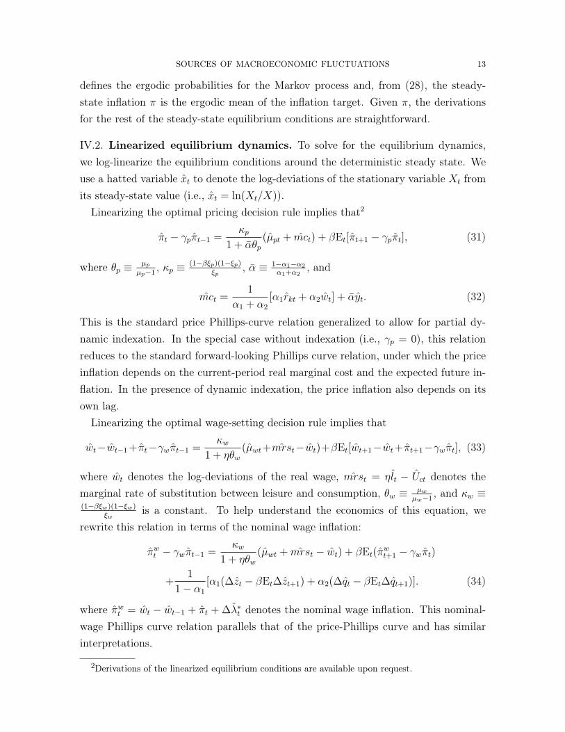
Linearizing the optimal pricing decision rule implies that2
πt − γpπt−1 =κp
1 + αθp
(µpt + mct) + βEt[πt+1 − γpπt], (31)
where θp ≡ µp
µp−1, κp ≡ (1−βξp)(1−ξp)
ξp, α ≡ 1−α1−α2
α1+α2, and
mct =1
α1 + α2
[α1rkt + α2wt] + αyt. (32)
This is the standard price Phillips-curve relation generalized to allow for partial dy-namic indexation. In the special case without indexation (i.e., γp = 0), this relationreduces to the standard forward-looking Phillips curve relation, under which the priceinflation depends on the current-period real marginal cost and the expected future in-flation. In the presence of dynamic indexation, the price inflation also depends on itsown lag.
Linearizing the optimal wage-setting decision rule implies that
wt−wt−1+πt−γwπt−1 =κw
1 + ηθw
(µwt+mrst−wt)+βEt[wt+1−wt+πt+1−γwπt], (33)
where wt denotes the log-deviations of the real wage, mrst = ηlt − Uct denotes themarginal rate of substitution between leisure and consumption, θw ≡ µw
µw−1, and κw ≡
(1−βξw)(1−ξw)ξw
is a constant. To help understand the economics of this equation, werewrite this relation in terms of the nominal wage inflation:
πwt − γwπt−1 =
κw
1 + ηθw
(µwt + mrst − wt) + βEt(πwt+1 − γwπt)
+1
1 − α1
[α1(∆zt − βEt∆zt+1) + α2(∆qt − βEt∆qt+1)]. (34)
where πwt = wt − wt−1 + πt + ∆λ∗
t denotes the nominal wage inflation. This nominal-wage Phillips curve relation parallels that of the price-Phillips curve and has similarinterpretations.
2Derivations of the linearized equilibrium conditions are available upon request.

SOURCES OF MACROECONOMIC FLUCTUATIONS 14
The rest of the linearized equilibrium conditions are summarized below:
qkt = S ′′(λI)λ2I
{∆it − βEt∆it+1
+1
1 − α1
[α2(∆zt − βEt∆zt+1) + ∆qt − βEt∆qt+1]
}, (35)
qkt = Et
{∆at+1 + ∆Uc,t+1 −
1
1 − α1
[α2∆zt+1 + ∆qt+1]
+β
λI
[(1 − δ)qk,t+1 − δδt+1 + rkrk,t+1
]}, (36)
rkt = σuut, (37)
0 = Et
[∆at+1 + ∆Uc,t+1 −
1
1 − α1
[α2∆zt+1 + α1∆qt+1] + Rt − πt+1
], (38)
kt =1 − δ
λI
[kt−1 −
1
1 − α1
(α2∆zt + ∆qt)
]− δ
λI
δt +
(1 − 1 − δ
λI
)it, (39)
yt = cy ct + iy it + uyut + gygt, (40)
yt = α1
[kt−1 + ut −
1
1 − α1
(α2∆zt + ∆qt)
]+ α2lt, (41)
wt = rkt + kt−1 + ut −1
1 − α1
(α2∆zt + ∆qt) − lt, (42)
where (35) is the linearized investment decision equation with qkt denoting the shadowvalue of existing capital (i.e., Tobin’s Q) and the ∆ denoting the first-difference operator(so that ∆xt = xt − xt−1); (36) is the linearized capital Euler equation; (37) is thelinearized capacity utilization decision equation with σu ≡ a′′(1)
a′(1)denoting the curvature
the function a(u) evaluated at the steady state; (38) is the linearized bond Eulerequation; (39) is the linearized law of motion for the capital stock; (40) is the linearizedaggregate resource constraint, with the steady-state ratios given by cy = C
Y, iy = I
Y,
uy = rkK
Y λI, and gy = G
Y; (41) is the linearized aggregate production function; and (42)
is the linearized factor demand relation.Finally, the linearized interest rate rule is given by
Rt = ρrRt−1 + (1 − ρr) [ϕπ(πt − π∗(st)) + ϕyyt] + σrtεrt, (43)
where the term π∗(st) ≡ log π∗(st)− log π denotes the deviations of the inflation targetfrom its ergodic mean.
V. Estimation Approach
We estimate the parameters in our model using the Bayesian method. We describe ageneral empirical strategy so that the method can be applied to other regimes-switching
SOURCES OF MACROECONOMIC FLUCTUATIONS 15
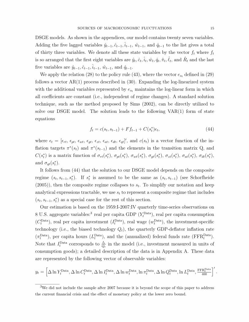
DSGE models. As shown in the appendices, our model contains twenty seven variables.Adding the five lagged variables yt−1, ct−1, it−1, wt−1, and qt−1 to the list gives a totalof thirty three variables. We denote all these state variables by the vector ft where ft
is so arranged that the first eight variables are yt, ct, it, wt, qt, πt, ℓt, and Rt and the lastfive variables are yt−1, ct−1, it−1, wt−1, and qt−1.
We apply the relation (28) to the policy rule (43), where the vector est defined in (29)follows a vector AR(1) process described in (30). Expanding the log-linearized systemwith the additional variables represented by est maintains the log-linear form in whichall coefficients are constant (i.e., independent of regime changes). A standard solutiontechnique, such as the method proposed by Sims (2002), can be directly utilized tosolve our DSGE model. The solution leads to the following VAR(1) form of stateequations
ft = c(st, st−1) + Fft−1 + C(s∗t )ϵt, (44)
where ϵt = [ϵrt, ϵpt, ϵwt, ϵgt, ϵzt, ϵat, ϵdt, ϵqt]′, and c(st) is a vector function of the in-
flation targets π∗(st) and π∗(st−1) and the elements in the transition matrix Q, andC(s∗t ) is a matrix function of σrt(s
∗t ), σpt(s
∗t ), σwt(s
∗t ), σgt(s
∗t ), σzt(s
∗t ), σat(s
∗t ), σdt(s
∗t ),
and σqt(s∗t ).
It follows from (44) that the solution to our DSGE model depends on the compositeregime (st, st−1, s
∗t ). If s∗t is assumed to be the same as (st, st−1) (see Schorfheide
(2005)), then the composite regime collapses to st. To simplify our notation and keepanalytical expressions tractable, we use st to represent a composite regime that includes(st, st−1, s
∗t ) as a special case for the rest of this section.
Our estimation is based on the 1959:I-2007:IV quarterly time-series observations on8 U.S. aggregate variables:3 real per capita GDP (Y Data
t ), real per capita consumption(CData
t ), real per capita investment (IDatat ), real wage (wData
t ), the investment-specifictechnology (i.e., the biased technology Qt), the quarterly GDP-deflator inflation rate(πData
t ), per capita hours (LDatat ), and the (annualized) federal funds rate (FFRData
t ).Note that IData
t corresponds to It
Qtin the model (i.e., investment measured in units of
consumption goods); a detailed description of the data is in Appendix A. These dataare represented by the following vector of observable variables:
yt =[∆ ln Y Data
t , ∆ ln CDatat , ∆ ln IData
t , ∆ ln wDatat , ln πData
t , ∆ ln QDatat , ln LData
t , FFRDatat
400
]′.
3We did not include the sample after 2007 because it is beyond the scope of this paper to addressthe current financial crisis and the effect of monetary policy at the lower zero bound.
SOURCES OF MACROECONOMIC FLUCTUATIONS 16
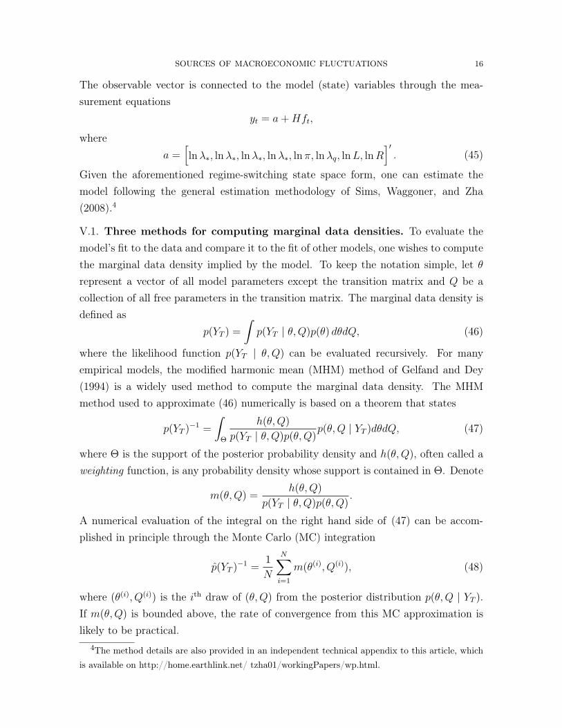
The observable vector is connected to the model (state) variables through the mea-surement equations
yt = a + Hft,
wherea =
[ln λ∗, ln λ∗, ln λ∗, ln λ∗, ln π, ln λq, ln L, ln R
]′. (45)
Given the aforementioned regime-switching state space form, one can estimate themodel following the general estimation methodology of Sims, Waggoner, and Zha(2008).4
V.1. Three methods for computing marginal data densities. To evaluate themodel’s fit to the data and compare it to the fit of other models, one wishes to computethe marginal data density implied by the model. To keep the notation simple, let θ
represent a vector of all model parameters except the transition matrix and Q be acollection of all free parameters in the transition matrix. The marginal data density isdefined as
p(YT ) =
∫p(YT | θ, Q)p(θ) dθdQ, (46)
where the likelihood function p(YT | θ,Q) can be evaluated recursively. For manyempirical models, the modified harmonic mean (MHM) method of Gelfand and Dey(1994) is a widely used method to compute the marginal data density. The MHMmethod used to approximate (46) numerically is based on a theorem that states
p(YT )−1 =
∫Θ
h(θ,Q)
p(YT | θ,Q)p(θ, Q)p(θ, Q | YT )dθdQ, (47)
where Θ is the support of the posterior probability density and h(θ,Q), often called aweighting function, is any probability density whose support is contained in Θ. Denote
m(θ, Q) =h(θ,Q)
p(YT | θ,Q)p(θ, Q).
A numerical evaluation of the integral on the right hand side of (47) can be accom-plished in principle through the Monte Carlo (MC) integration
p(YT )−1 =1
N
N∑i=1
m(θ(i), Q(i)), (48)
where (θ(i), Q(i)) is the ith draw of (θ,Q) from the posterior distribution p(θ,Q | YT ).If m(θ,Q) is bounded above, the rate of convergence from this MC approximation islikely to be practical.
4The method details are also provided in an independent technical appendix to this article, whichis available on http://home.earthlink.net/ tzha01/workingPapers/wp.html.
SOURCES OF MACROECONOMIC FLUCTUATIONS 17
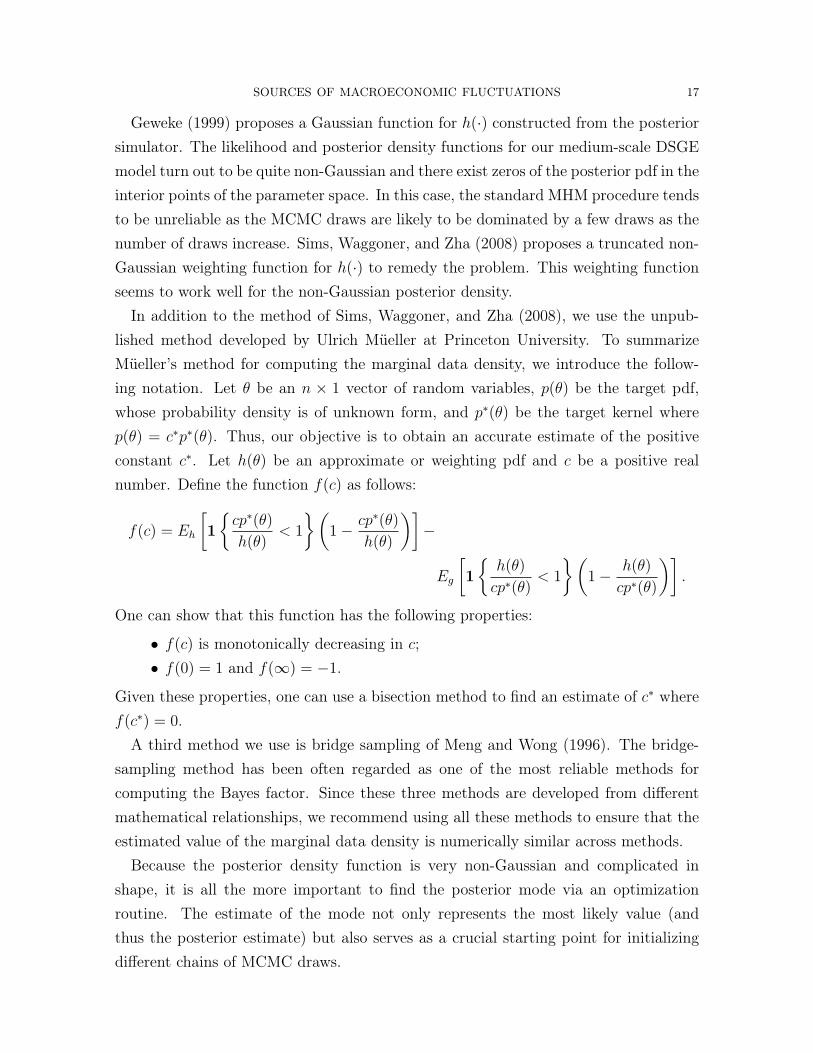
Geweke (1999) proposes a Gaussian function for h(·) constructed from the posteriorsimulator. The likelihood and posterior density functions for our medium-scale DSGEmodel turn out to be quite non-Gaussian and there exist zeros of the posterior pdf in theinterior points of the parameter space. In this case, the standard MHM procedure tendsto be unreliable as the MCMC draws are likely to be dominated by a few draws as thenumber of draws increase. Sims, Waggoner, and Zha (2008) proposes a truncated non-Gaussian weighting function for h(·) to remedy the problem. This weighting functionseems to work well for the non-Gaussian posterior density.
In addition to the method of Sims, Waggoner, and Zha (2008), we use the unpub-lished method developed by Ulrich Müeller at Princeton University. To summarizeMüeller’s method for computing the marginal data density, we introduce the follow-ing notation. Let θ be an n × 1 vector of random variables, p(θ) be the target pdf,whose probability density is of unknown form, and p∗(θ) be the target kernel wherep(θ) = c∗p∗(θ). Thus, our objective is to obtain an accurate estimate of the positiveconstant c∗. Let h(θ) be an approximate or weighting pdf and c be a positive realnumber. Define the function f(c) as follows:
f(c) = Eh
[1
{cp∗(θ)
h(θ)< 1
}(1 − cp∗(θ)
h(θ)
)]−
Eg
[1
{h(θ)
cp∗(θ)< 1
}(1 − h(θ)
cp∗(θ)
)].
One can show that this function has the following properties:
• f(c) is monotonically decreasing in c;• f(0) = 1 and f(∞) = −1.
Given these properties, one can use a bisection method to find an estimate of c∗ wheref(c∗) = 0.
A third method we use is bridge sampling of Meng and Wong (1996). The bridge-sampling method has been often regarded as one of the most reliable methods forcomputing the Bayes factor. Since these three methods are developed from differentmathematical relationships, we recommend using all these methods to ensure that theestimated value of the marginal data density is numerically similar across methods.
Because the posterior density function is very non-Gaussian and complicated inshape, it is all the more important to find the posterior mode via an optimizationroutine. The estimate of the mode not only represents the most likely value (andthus the posterior estimate) but also serves as a crucial starting point for initializingdifferent chains of MCMC draws.

SOURCES OF MACROECONOMIC FLUCTUATIONS 18
For various DSGE models studied in this paper, finding the mode has proven tobe a computationally challenging task. The optimization method we use combinesthe block-wise BFGS algorithm developed by Sims, Waggoner, and Zha (2008) andvarious constrained optimization routines contained in the commercial IMSL package.The block-wise BFGS algorithm, following the idea of Gibbs sampling and EM algo-rithm, breaks the set of model parameters into subsets and uses Christopher A. Sims’scsminwel program to maximize the likelihood of one set of the model’s parametersconditional on the other sets.5 Maximization is iterated at each subset until it con-verges. Then the optimization iterates between the block-wise BFGS algorithm andthe IMSL routines until it converges. The convergence criterion is the square root ofmachine epsilon.
Thus far we have described the optimization process for only one starting point.6
Our experience is that without such a thorough search, one can be easily misled to amuch lower posterior value (e.g., a few hundreds lower in log value than the posteriorpeak). We thus use a set of cluster computing tools described in Ramachandran,Urazov, Waggoner, and Zha (2007) to search for the posterior mode. We begin with agrid of 100 starting points; after convergence, we perturb each maximum point in bothsmall and large steps to generate additional 20 new starting points and restart theoptimization process again; the posterior estimates attain the highest posterior densityvalue. The other converged points typically have much lower likelihood values by atleast a magnitude of hundreds of log values. For each DSGE model, the peak value ofthe posterior kernel and the mode estimates are reported.
V.2. Priors. We set three parameters a priori. We set the steady-state governmentspending to output ratio at gy = 0.18. We follow Justiniano and Primiceri (2006)and fix the persistence of the government spending shock process at ρg = 0.99. Asnoted by Smets and Wouters (2007), all these government parameter are difficult toestimate unless government spending is included in the set of measurement equations.Finally, we normalize and fix the steady-state hours worked at L = 0.2. We estimateall the remaining parameters. Tables 3 and 4 summarize the prior distributions for thestructural parameters and the shock parameters.
5The csminwel program can be found on http://sims.princeton.edu/yftp/optimize/.6For the no-switching (constant-parameter) DSGE model, it takes a couple of hours to find the
posterior peak. While the model with two-regime shock variances takes about 20 hours to converge,the model with two-regime inflation targets and two-regime two-regime shock variances takes fourtimes longer.

SOURCES OF MACROECONOMIC FLUCTUATIONS 19
Our priors are chosen to be more flexible and less tight than those in the previousliterature. Specifically, instead of specifying the mean and the standard deviation, weuse the 90% probability interval to back out the hyperparameter values of the priordistribution.7 The intervals are generally set wide enough to allow the possibility ofmultiple posterior peaks (Del Negro and Schorfheide, 2008). Our approach is also nec-essary to deal with skewed distributions and allow for some reasonable hyperparametervalues in certain distributions (such as the Inverse-Gamma) where the first two mo-ments may not exist. The probability intervals reported in Table 3 cover the calibratedvalue of each parameter.
We begin with the preference parameters b, η, and β. Our prior for the habit-persistence parameter b follows the Beta distribution. We choose the 2 hyper-parametersof the Beta distribution such that the lower bound for b (0.05) has a cumulative prob-ability of 5% and the upper bound (0.948) has a cumulative probability of 95%. This90% probability interval for b covers the values used by most economists (for exam-ple, Boldrin, Christiano, and Fisher (2001) and Christiano, Eichenbaum, and Evans(2005)). Our prior for the inverse Frisch elasticity η follows the Gamma distribution.We choose the 2 hyper-parameters of the Gamma distribution such that the lowerbound (0.2) and the upper bound (10.0) of η correspond to the 90% probability in-terval. This prior range for η implies that the Frisch elasticity lies between 0.1 and5, a range broad enough to cover the values based on both microeconomic evidence(Pencavel, 1986) and macroeconomic studies (Rupert, Rogerson, and Wright, 2000).Our prior for the transformed subjective discount factor χβ ≡ 100( 1
β− 1) follows the
Gamma distribution, with the hyper-parameters appropriately chosen such that thebounds for the 90% probability interval of χβ are 0.2 and 4.0. The implied value of β
lies in the range between 0.9615 and 0.998, which nests the values obtained by Smetsand Wouters (2007) (β = 0.9975) and Altig, Christiano, Eichenbaum, and Linde (2004)(β = 0.9926).
Next, we discuss the prior distributions for the technology parameters α1, α2, λq, λ∗,σu, S ′′, and δ. Our priors for the labor share and capital share both follow the Betadistribution with the restriction α1 +α2 ≤ 1 so that the production technology requiresfirm-specific factors (Chari, Kehoe, and McGrattan, 2000). Specifically, the bounds forthe α1 values in the 90% probability interval are 0.15 and 0.35 and those for α2 are0.35 and 0.75. With the restriction α1 + α2 ≤ 1, however, the joint 90% probability
7The program for backing out the hyperparameter values of a given prior can be found inhttp://home.earthlink.net/ tzha02/ProgramCode/programCode.html.

SOURCES OF MACROECONOMIC FLUCTUATIONS 20
region would be somewhat different. We assume that the priors for the (transformed)trend growth rates of the investment-specific technology and the neutral technologyboth follow the Gamma distribution, with the 5% and 95% bounds given by 0.1 and1.5 respectively. These values imply that, with 90% probability, the prior values for thetrend growth rates λq and λ∗ lie in the range between 1.001 and 1.015 (correspondingto annual rates of 0.4% and 6%, respectively). We assume that the priors for thecapacity utilization parameter σu and the investment adjustment cost parameter S ′′
both follow the Gamma distribution, with the lower bounds given by 0.5 and 0.1 andthe upper bounds given by 3.0 and 5.0, respectively. These 90% probability rangescover the values obtained, for example, by Christiano, Eichenbaum, and Evans (2005)and Smets and Wouters (2007). We assume that the prior for the average annualizeddepreciation rate follows the Beta distribution with the 90% probability range lyingbetween 0.05 and 0.20.
Third, we discuss the prior distributions for the parameters that characterize priceand nominal wage setting in the model. These include the average price markup µp,the average wage markup µw, the Calvo probabilities of non-adjustment in pricing ξp
and in wage-setting ξw, and the indexation parameters γp and γw. The priors for thenet markups µp − 1 and µw − 1 both follow the Gamma distribution with the 90%
probability range covering the values between 0.01 and 0.5. This range covers most ofthe calibrated values of the markup parameters used in the literature (e.g., Basu andFernald (2002), Rotemberg and Woodford (1997), Huang and Liu (2002)). The priorsfor the price and wage duration parameters ξp and ξw both follow the Beta distributionwith the 90% probability range between 0.1 and 0.75. Under this prior distribution,the nominal contract durations vary, with 90% probability, between 1.1 quarters and 4
quarters. This range covers the values of the frequencies of price and wage adjustmentsused in the literature (e.g., Bils and Klenow (2004), Taylor (1999)). The priors for theindexation parameters γp and γw both follow the uniform distribution with the 90%
probability range lying between 0.05 and 0.95. In this sense, we have loose priors onthese indexation parameters, the range of which covers those used in most studies (e.g.,Christiano, Eichenbaum, and Evans (2005), Smets and Wouters (2007), and Woodford(2003)).
Finally, we discuss the coefficients in the monetary policy rule, including ρr, ϕπ, andϕy. The prior for the interest-rate smoothing parameter ρr follows the Beta distributionwith the 90% probability range between 0.05 and 0.948. The prior for the inflationcoefficient ϕπ follows the Gamma distribution with the 90% probability range between
SOURCES OF MACROECONOMIC FLUCTUATIONS 21
0.5 and 5.0. The prior for the output coefficient ϕy follows the Gamma distributionwith the 90% probability range between 0.05 and 3.0. This range includes the valuesobtained by Clarida, Galí, and Gertler (2000) and others. These prior values allowfor an indeterminacy region. When the equilibrium is indeterminate, we follow Boivinand Giannoni (2006) and use the MSV solution. In our estimation, however, there ispractically little probability for the parameters to be in the indeterminate region.
Our priors for the AR(1) coefficients for the neutral and biased technology shocksρq and ρz are uniformly distributed in the [0, 1] interval. The AR(1) coefficients for allother shocks and the MA(1) coefficients for the price and wage markup shocks followthe Beta distribution with the 5%-95% probability range given by [0.05, 0.948]. Theprior for the parameter ρgz follows the Gamma distribution with the 90% probabilityrange given by [0.2, 3.0]. The standard deviations of each of the 8 shocks follow theInverse Gamma distribution with the 90% probability range given by [0.0005, 1.0]. Thisprobability range implies a more agnostic prior than Smets and Wouters (2007) andJustiniano and Primiceri (2006). Such an agnostic prior is needed to allow for possiblelarge changes in shock variances across regimes, as found in Sims and Zha (2006).
We have experimented with different priors. In one alternative prior, we follow theliterature and make a prior on the persistence parameters in shock processes muchtighter towards zero, such as the Beta(1, 2) probability density. Our conclusions holdtrue for these priors as well.
VI. Empirical Results
In this section, we report our main empirical findings. We compare in Section VI.1the empirical fit of a variety of models nested by our general regime-switching DSGEframework. We then report in Section VI.2 the estimation results in our best-fit modeland highlight the difference of these estimates from some alternative models.
VI.1. Model Fit. The first set of results to discuss is measures of model fit, withthe comparison based on maximum log posterior densities adjusted by the Schwarzcriterion.8 Table 1 reports Schwarz criteria for different versions of our DSGE model(the column “Baseline”) and for models with the restriction that all the persistenceparameters in both price markup and wage markup processes are set to zero (thecolumn “Restricted”).
8The Schwarz criterion is similar to the Laplace approximation used by Smets and Wouters (2007).

SOURCES OF MACROECONOMIC FLUCTUATIONS 22
Table 1 shows that the model with regime shifts in shock variances only (DSGE-2v)is the best-fit model, much better than the constant-parameter DSGE model (DSGE-con). The Schwarz criterion for the baseline DSGE-2v model is 5963.03, comparedto 5859.71 for the DSGE-con model. When we allow the inflation target to switchregimes while holding the shock variances constant (DSGE-2c), the model’s fit doesnot improve upon the constant-parameter DSGE model. When we allow both theinflation target and shock variances to switch regimes with the same Markov process(i.e., regime switching is synchronized), the model (DSGE-2cv) does better than theone with regime switching in the inflation target alone, but it does not improve uponthe baseline DSGE-2v model with regime shifts in the shock variances only. Whenwe relax the assumption that switches in the shock regime and those in the inflationtarget regime are synchronized and compute the Schwarz criterion for the model withthe target regime and the shock regime independent of each other (DSGE-2c2v), wefind that the model’s fit does not improve relative to either the DSGE-2cv model withsynchronized regime shifts in the inflation target and the shock variances or the baselineDSGE-2v model with synchronized regime shifts in shock variances only. We have alsoexamined the possibility of 3 shock regimes instead of 2. We find that the 3-regimemodel (DSGE-3v) does not improve upon the baseline 2-regime model (DSGE-2v).
We have also estimated models with shock variances following independent Markovswitching processes. This scenario approximates stochastic volatility models, whereeach shock variance has its own independent stochastic process (Tauchen, 1986; Sims,Waggoner, and Zha, 2008). In addition, we have grouped a subset of shock varianceshaving the same Markov processes. None of these models fits to the data better thanour baseline DSGE-2v model. For example, when we allow regimes associated withthe variances of the two technology shocks to be independent of the regime switchingprocesses of the other shock variances (DSGE-2v2v), we obtain a Schwarz criterion of5958.18, which is lower than that of the baseline DSGE-2v model (5963.03). In short,the data favor the parsimoniously-parameterized model with shock variances switchingregimes simultaneously.
The last column in Table 1 shows that the model with regime changes in shock vari-ances only continues to dominate all the other models, when the persistence parametersin both price and wage markup shock processes are restricted to zero. In particular,the model with the target switching regimes (DSGE-2c) does not improve upon theconstant-parameter model. Of course, all these restricted models fit to the data much

SOURCES OF MACROECONOMIC FLUCTUATIONS 23
worse than the corresponding baseline models, implying that persistent shock processesare important in fitting the data.
Finally, we have estimated a number of models with persistence parameters in othershock processes set to zero and with habit and indexation parameters set to zero.The model with synchronized regimes in shock variances continue to outperform othermodels in fitting the data.
The relative performance of the alternative DSGE models in fitting the data does notchange when we look at the marginal data density (MDD). Table 2 reports the MDDfor each of the alternative models. The table shows that the model with simultaneousregime shifts in shock variances (DSGE-2v) is the best-fit model not only in termsof the Schwarz criterion, but also in terms of the marginal data density. In particu-lar, the DSGE-2v model’s MDD is 5832.38, much higher than that of the DSGE-conmodel (whose MDD is 5741.24). The model with regime switching in the inflationtarget alone (DSGE-2c) slightly outperforms the constant parameter model, but sub-stantially under-performs the DSGE-2v model. With regime shifts in shock variances,introducing regime shifts in the inflation target synchronized with regime shifts inshock variances (DSGE-2cv) or allowing the inflation target to follow a Markov switch-ing process independent of shock regimes (DSGE-2c2v) does not improve the marginaldata density relative to the DSGE-2v model.9
VI.2. Estimates of Structural Parameters. We first discuss our best-fit model“DSGE-2v.” The model is similar to that in Smets and Wouters (2007) with six notableexceptions. First, we introduce a source of real rigidity in the form of firm-specificfactors, which replaces the kinked demand curves considered by Smets and Wouters(2007). Second, we introduce trend growth in the investment-specific technologicalchange to better capture the data, in which the relative price of investment goods(e.g., equipment and software) has been declining for most of the postwar period,while in Smets and Wouters (2007) the investment-specific technological changes haveno trend component. We use the observed time series of biased technological changesin our estimation, while Smets and Wouters (2007) treat these changes as a latentvariable. Third, we introduce the depreciation shock that acts as a wedge in thecapital-accumulation Euler equation. Fourth, the preference shock in our model entersall intertemporal decisions, including choices of the nominal bond, the capital stock,
9The good fit represented by DSGE-2cv comes entirely from significant shifts in shock variances.The estimated inflation targets are 2.18% for one regime and 1.70% for the other regime and thedifference between these two targets are statistically insignificant.

SOURCES OF MACROECONOMIC FLUCTUATIONS 24
and investment, while Smets and Wouters (2007) introduce a “risk-premium shock” thatenters the bond Euler equation only and does not affect other intertemporal decisions.Fifth, in the interest rate rule, we assume that the nominal interest rate respondsto deviations of inflation from its target and detrended output, while in Smets andWouters (2007) the interest rate rule targets inflation, output gap, and the growth rateof output gap. Finally, we allow for heteroscadasticity of structural shocks to obtainthe accurate estimate of the role of a particular shock in explaining macroeconomicfluctuations. All these distinctions may explain some of the differences between ourestimated results and theirs.
Tables 3 and 4 report the estimates of the model parameters. The data are informa-tive about many structural parameters. Among the three preference parameters, theestimate for habit persistence (b) is 0.91 with the tight error bands. The estimate forη is 2.89, implying a Frisch elasticity of 0.35 and consistent with most microeconomicstudies. The probability interval indicates that η can be as high as 8.38. The estimatefor the subjective discount factor β is 0.998 (the same as the value obtained by Smetsand Wouters (2007)) with the tight probability interval [0.996, 0.999].
Among the technology parameters, the estimate for α1 (0.153) with the upper er-ror band (0.216) close to the estimate obtained by Smets and Wouters (2007) (0.19).Because of the constraint α1+α2 ≤ 1, the estimate for α2 is (0.835). These posterior es-timates suggest that the data prefer a model specification with (near) constant-returnsproduction technology. The estimated trend growth rate for the investment-specifictechnological change (λq) is 4% per annum, slightly higher than the calibrated valueobtained by Greenwood, Hercowitz, and Krusell (1997) because we include the datain the late 1990s until 2007 when the investment-specific technological improvementwas the fastest in the sample. The estimate for the trend growth rate of the neutraltechnological change (λ∗) is 0.95% per annum. There is a large amount of uncertaintyabout these trend estimates as shown in the last two columns of Table 3. The cur-vature parameter in the utilization function (σu) is estimated at 2.26, substantiallylower than the value obtained by Justiniano and Primiceri (2006) (7.13), but higherthan the values estimated by Altig, Christiano, Eichenbaum, and Linde (2004) (2.02)and by Smets and Wouters (2007) (1.174). The error bands show a large amount ofuncertainty around the estimate of this parameter. The investment adjustment costparameter (S ′′) is estimated to be 2.0, lower than those obtained in the literature.Unlike most studies in the literature that fix the value of the capital depreciation ratea priori, we allow the depreciation rate δ to follow a stationary stochastic process and

SOURCES OF MACROECONOMIC FLUCTUATIONS 25
estimate the parameter in the process. The estimated average annum depreciation rateis 13.4%, which is remarkably close to the standard calibration value in the real busi-ness cycle literature, but the error bands are very wide, implying the great uncertaintyabout this estimate.
Among the pricing and wage setting parameters, the estimated average price markup(µp) is about 1.0, which is consistent with the studies by Hall (1988), Basu and Fernald(1997), and Rotemberg and Woodford (1999), who argue that the pure economic profitis close to zero. It is also similar to the estimate obtained by Altig, Christiano, Eichen-baum, and Linde (2004), but much smaller than the value estimated by Justiniano andPrimiceri (2006). Our estimate for the average wage markup (µw) is 1.06, which is lowerthan the calibrated value (Huang and Liu, 2002) and the estimated value (Justinianoand Primiceri, 2006), but is similar to the value used by Christiano, Eichenbaum, andEvans (2005). The uncertainty about the wage markup parameter, judged by the .90probability bands, is much larger than that about the price markup parameter. Theestimated price and wage stickiness parameters (ξp = 0.412 and ξw = 0.213) imply that,on average, price contracts last for less than 2 quarters and nominal wage contractshave an even shorter duration, which is slightly more than 1 quarter. Our estimatednominal contract duration is consistent with the microeconomic studies such as Bilsand Klenow (2004). The estimated dynamic indexation is unimportant for price set-ting (γp = 0.178) but very important for nominal wage setting (γw = 1.0). The .90probability intervals indicate that while the price indexation is tightly estimated, theuncertainty about the nominal wage indexation is extremely large.
As shown in Tables 3, the estimated wage stickiness parameter lies below the lowerbound of the .90 probability interval. This phenomenon occurs because the posteriordistribution around the mode for this parameter is on the thin ridge and because thereare many local peaks that give a significant probability to regions containing the valuesabove the estimated wage stickiness parameter. While it is impossible to graph thisphenomenon in a high dimensional parameter space like ours, we display in Figure 1the joint distribution of the wage stickiness parameter and the average wage markupparameter after integrating out all other parameters. As one can see, the multiplelocal peaks give much of the probability to the values of the wage stickiness param-eters greater than the estimate at the posterior mode. Because the two-dimensionaldistribution displayed in Figure 1 integrates out all other parameters, the distributionis already skewed toward the values of the wage stickiness parameters greater than 0.2.
SOURCES OF MACROECONOMIC FLUCTUATIONS 26
Nonetheless, the picture demonstrates clearly the nature of thin ridges and multiplelocal peaks inherent in the posterior distribution.
The estimates of policy parameters suggest that interest-rate smoothing is important;the estimate of ρr is 0.82 with a narrow probability interval. The policy responseto deviations of inflation from its target in the interest rule (ϕπ) is 1.655 with thelower probability bound still significantly above 1.0. Policy does not respond much todetrended output and the parameter (ϕy) is tightly estimated. The inflation target(π∗) is estimated at 2.28% per annum.
The estimated results for shock processes are reported in Table 4. The AR(1) co-efficients for all shocks except the preference shock (ρa) are above 0.9, although thelower probability bounds for some coefficients are substantially below (0.9). The pref-erence shock is almost i.i.d.. The MA(1) coefficients in the price markup and wagemarkup processes (ϕp and ϕw) are both sizable. The estimates are 0.698 and 0.749 andthe corresponding .90 probability intervals support these high values. The governmentspending shock responds to the neutral technology shock; the response coefficient (ρgz)is 0.894 with a wide probability interval. Although the prior distributions for all theshock variances are the same, the posterior estimates are very disperse. The depre-ciation shock (σd) and the wage markup shock (σw) have the largest variances; themonetary policy shock (σr) and the two types of technology shocks (σz and σq) havethe smallest variances. The .90 probability intervals indicate that the marginal poste-rior distribution of a shock variance is skewed to the right. This shape is expected asthe variance is bounded below by zero below and has no upward bound.
As shown in Table 4, the estimated shock variances in the second regime are sub-stantially smaller than those in the first regime. The estimated transition probabilitiesare summarized by the matrix
Q =
[0.8072 0.0598
0.1928 0.9402
], (49)
where the elements in each column sum to one. The second regime (i.e., the regimewith low shock variances) is more persistent and, as shown in Figure 2, covers mostof the period since Greenspan became Chairman of the Federal Reserve Board. Thisresult is even stronger when one take into account the error bands, where the lowerbound of q22 is higher than the upper bound of q11.
Figure 3 plots the marginal posterior distribution of some key parameters. The localpeaks shown in the marginal distribution of the inflation target are the direct outcomeof the integrated effect of the non-Gaussian joint posterior distribution of all parameters

SOURCES OF MACROECONOMIC FLUCTUATIONS 27
that has thin ridges and multiple peaks. Most of the probability, however, concentratesbetween 2% and 4%. The marginal distribution of the response coefficient to inflation inthe Taylor indicates that there is practically no probability for indeterminate equilibriafor our model.
The marginal distribution of the price-stickiness parameter implies that the pricerigidity is much smaller than what is obtained in the previous literature. The posteriormode is near the lower tail of the marginal distribution. The joint distribution, asillustrated in Figure 1, has a thin ridge and many local peaks. After integrating outall other parameters, the marginal distribution of the wage-stickiness parameter showsa local peak around 0.7. The majority of the probability, however, lies below the value0.6.
There are two reasons why we obtain estimates that imply shorter durations of priceand wage contracts than those obtained in the literature such as Altig, Christiano,Eichenbaum, and Linde (2004) and Smets and Wouters (2007). First, our estimatessuggest that the price markup is very small, implying that the demand curve for dif-ferentiated goods is very flat. Thus, a small increase in the relative price can lead tolarge declines in relative output demand. Even if firms can re-optimize their pricingdecisions very frequently, they choose not to adjust their relative prices too much. Inthis sense, the small average markup and thus the large demand elasticity become asource of strategic complementarity in firms’ pricing decisions. Second, unlike Altig,Christiano, Eichenbaum, and Linde (2004) who use a minimum-distance estimator thatmatches the model’s impulse responses to those in the data, we use full-informationmaximum likelihood estimation. This difference is important because Altig, Chris-tiano, Eichenbaum, and Linde (2004) find that, while a shock to neutral technologyleads to rapid adjustments in prices, a shock to monetary policy leads to small andgradual price adjustments. Under their estimation approach, matching the impulseresponses following the monetary policy shock is important so that price adjustmentshave to be small and gradual. Our estimation approach differs from theirs and we findthat the most important shocks are those to neutral technology, capital depreciation,and wage markup, all of which lead to rapid adjustments in prices. Consequently, ourestimated durations of nominal contracts are shorter than those in the literature.
The last row of Figure 3 displays the marginal posterior distributions of the invest-ment technology trend and the wage indexation. The distribution of the investmenttechnology trend puts a significant amount of probability around 4%, consistent with

SOURCES OF MACROECONOMIC FLUCTUATIONS 28
the data on the relative price of investment. The distribution of the wage indexa-tion parameter is most interesting. While the estimate is at 1.0, there is considerableuncertainty around the wage indexation parameter so that the estimate of 1.0 is veryimprecise. This result implies that our estimation does not necessarily support a strongwage indexation.
VII. Economic Implications
We now discuss the economic implications of our best-fit model. We first examine,in Section VII.1, the role of the various shocks in driving macroeconomic fluctuationsthrough variance decompositions. We then present, in Section VII.2, impulse responsesof several key aggregate variables to each of the shocks that we identify as importantfor macroeconomic fluctuations. Finally, we provide some economic interpretations ofthe key sources of shocks and in particular, the capital depreciation shock.
VII.1. Variance decompositions. Tables 5 and 6 report variance decompositions inforecast errors of output, investment, hours, the real wage, and inflation under thetwo shock regimes at different forecasting horizons for our best-fit model. As we havediscussed in Section VI.2, the wage markup shock and the depreciation shock have thelargest variances among all eight structural shocks. The neutral technology shock isof considerable interest because of the debate in the recent literature on its dynamiceffects on the labor market variables (e.g., Galí (1999), Christiano, Eichenbaum, andVigfusson (2003), Uhlig (2004), and Liu and Phaneuf (2007)).
As we can see, capital depreciation shocks, neutral technology shocks, and wagemarkup shocks play an important role in driving business cycle fluctuations underboth regimes. Taken together, these three types of shocks account for 70 − 80% ofthe fluctuations in output, investment, hours, and inflation under each regime for theforecast horizons beyond eight quarters. Monetary policy shock accounts for a sizablefraction of inflation fluctuations under the first regime but otherwise it is unimportant.The price markup shock contributes to about 15 − 30% of the real wage fluctuationsunder both regimes. It is also somewhat important for inflation fluctuations under thesecond regime. The remaining three shocks, including the government spending shock,the preference shock, and the biased technology shock are unimportant in explainingmacroeconomic fluctuations.
VII.2. Impulse responses. To gain intuition about the model’s transmission mech-anisms, we analyze impulse responses of selected variables following some of the struc-tural shocks. In particular, we focus on the dynamic effects of a wage markup shock,

SOURCES OF MACROECONOMIC FLUCTUATIONS 29
a neutral technology shock, and a depreciation shock on output, investment, the realwage, the inflation rate, hours, and the nominal interest rate. These shocks, as we dis-cuss in the previous section, are the most important driving sources of macroeconomicfluctuations. Since the impulse responses display the same patterns for both shockregimes except the scaling effect, we report the impulse responses only for the secondregime.
Figure 4 displays the impulse responses following a one-standard-deviation shockto the capital depreciation rate. The increase in the depreciation rate reduces thevalue of capital accumulation and raises utilization and the rental price of capital;thus investment falls. Since the expected stock of capital wealth declines, the negativewealth effect leads to a fall in consumption as well. Consequently, aggregate outputfalls. The decline in output leads to a decline in hours. The decline in hours and inconsumption lowers the marginal rate of substitution between labor and consumption,so that the households’ desired wage falls. Thus, the equilibrium real wage declinesas well. The fall in the real wage reduces the firms’ marginal cost so that inflationdeclines. Through the Taylor rule, the nominal interest rate declines as well. As the.90 probability error bands show, all the responses are statistically significant.
Figure 5 reports the impulse responses following a one-standard-deviation shock tothe investment-specific technology. The biased shock raises the efficiency of investment,investment goods today become cheaper, and current consumption becomes more ex-pensive. This type of shock, unlike the depreciation shock or the neutral technologyshock, shifts resources from consumption to investment. Consequently, investmentrises and consumption declines. Hours declines initially due to the costly adjustmentin investment as well as the habit formation. After the second quarter, the increase indemand for investment gradually leads to a rise in hours and the real wage. The risein labor hours helps produce more output. Utilization and the rental price of capitalrise as well. All the responses are well estimated, judged by the .90 probability errorbands. In contrast to the responses to the depreciation shock, the biased technologyshock generates opposite movements in output and consumption in the short run andconsequently its impact on the macroeconomy is much smaller (by comparing the scalesin Figure 4 and those in Figure 5).
Both the capital depreciation shock and the investment-specific technology shockenter the intertemporal capital accumulation decision. But we find that this biased
SOURCES OF MACROECONOMIC FLUCTUATIONS 30
technology shock is much less important for macroeconomic fluctuations than the de-preciation shock. This finding is different from that in Justiniano, Primiceri, and Tam-balotti (2008), mainly because we use direct observations on the biased technologyshock in our estimation while they do not.
Figure 6 displays the impulse responses following a one-standard-deviation shock tothe neutral technology (i.e., the total factor productivity, or TFP). The positive neutraltechnology shock raises output, consumption, investment, utilization of capital, and thereal wage. All these responses are statistically significant for the most part. The shockshould lower inflation and, through the Taylor rule, the nominal interest rate. But theerror bands are wide so that the estimates are insignificant.
The neutral technology shock leads to a statistically significant decline in hoursworked. The decline in hours here, however, is not a direct consequence of pricestickiness. Even with much more frequent price adjustments, we find that the positiveneutral technology shock leads to a decline in hours (not reported). Instead, theinvestment adjustment cost (as well as the habit formation to a less extent) plays animportant role in generating the decline in hours. If the investment adjustment costparameter is small, we find that the model generates an increase in hours followingthe neutral technology shock (not reported), regardless of whether prices are sticky ornot. Thus, our finding does not support the view that the contractionary effect of aneutral technology shock arises from the price stickiness. It is consistent with Francisand Ramey (2005), who argue that a real business cycle model with habit persistenceand investment adjustment cost can generate a decline in hours following a positiveneutral technology shock.
Figure 7 reports the impulse responses following a one-standard-deviation shock tothe wage markup. An increase in the wage markup raises the households’ desired realwage. The households who can adjust their nominal wage raise their nominal wage.The increase in the nominal wage raises the firms’ marginal cost so that inflation risesand real aggregate demand falls. It follows that aggregate output, investment, andhours decline. Consequently, the rental price of capital and utilization rise. Throughthe interest-rate rule, the rise in inflation leads to an increase in the nominal interestrate. All these responses are statistically significant.
VII.3. What is a shock to capital depreciation? The variance decompositionsindicate that the TFP shock, the wage markup shock, and the depreciation shock arethe most important sources of macroeconomic fluctuations. The TFP shock and thewage markup shock should be familiar to many researchers, but the capital depreciation
SOURCES OF MACROECONOMIC FLUCTUATIONS 31
shock is new. Given its importance in accounting for the macroeconomic fluctuationsin our model, it is useful to provide economic interpretations of the depreciation shock.
Like the TFP shock or any other shocks in this class of models, the depreciationshock is of reduced form that captures some “deeper” sources of disturbances and pos-sibly microeconomic frictions that distort intertemporal capital accumulation decisions.Greenwood, Hercowitz, and Krusell (1997) draw a mapping between investment-specifictechnological changes and economic depreciation (as opposed to physical depreciation)of capital. They note that the economic depreciation rate rises when the equipmentprice relative to the consumption price is expected to decline in the future. As theequipment price is expected to fall, existing capital is worth less and investors haveincentive to postpone investment to future periods, leading to a contraction in currenteconomic activity, as does our depreciation shock.
Our depreciation shock also closely resembles the capital quality shock in Justiniano,Primiceri, and Tambalotti (2008) and Gertler and Kiyotaki (2010), who interpret theircapital quality shock as representing some exogenous changes in the value of capital.One possible microeconomic interpretation is that a large number of goods are producedusing good-specific capital. In each period, as a fraction of goods becomes obsoleterandomly, the capital used for producing those obsolete goods becomes worthless. Inaggregate, the law of motion for capital would feature a depreciation shock or similarlya capital quality shock to reflect the economic obsolescence of capital.
Thus, we view the depreciation shock as a stand in for economic obsolescence ofcapital. Unlike other intertemporal wedges such as the investment-specific technologyshock (or biased technology shock), the depreciation shock in our model generatespositive comovement between consumption, investment, hours, and the real wage. Ourempirical results in general suggest that the depreciation shock, along with the standardTFP shock and wage markup shock, is an important driving source of business cyclefluctuations in the U.S. economy.
VIII. Conclusion
We have studied a variety of fairly large DSGE models within a unified framework toreexamine the sources of observed macroeconomic fluctuations in the post-WWII U.S.economy. Our econometric estimation suggests that heteroscedasticity in shock distur-bances are important and that changes in shock variances take place simultaneouslyrather than independently. Three types of shocks stand out as the most important

SOURCES OF MACROECONOMIC FLUCTUATIONS 32
sources of macroeconomic volatilities: a depreciation shock that functions as an in-tertemporal wedge in capital accumulation, a total factor productivity shock that actsas an efficiency wedge, and a wage markup shock that serves as an intratemporal laborsupply wedge. We do not find evidence of changes in the inflation target, nor do wefind support for strong nominal rigidities in prices and nominal wages. These findingsare robust across a large set of regime-switching models.
Appendix A. Detailed Data Description
All data are either taken directly from the Haver Analytics Database or constructedby Patrick Higgins at the Federal Reserve Bank of Atlanta. The construction methodsdeveloped or used by Patrick Higgins, available on request, will be briefly describedbelow.
The model estimation is based on quarterly time-series observations on 8 U.S. aggre-gate variables during the sample period 1959:Q1–2007:Q4. The 8 variables are real percapita GDP (Y Data
t ), real per capita consumption (CDatat ), real per capita investment
(IDatat ) in capital goods, real wage (wData
t ), the quarterly GDP-deflator inflation rate(πData
t ), per capita hours (LDatat ), the federal funds rate (FFRData
t ), and the inverse ofthe relative price of investment (QData
t ).These series are derived from the original data in the Haver Analytics Database
(with the relevant data codes provided) or from the constructed data.
• Y Datat = GDPH
POP25-64 .• CData
t = (CN@USECON + CS@USECON)∗100/JGDPPOP25-64 .
• IDatat = (CD@USECON + F@USECON)∗100/JGDP
POP25-64 .• wData
t = LXNFC@USECON/100JGDP .
• πDatat = JGDPt
JGDPt−1.
• LDatat = LXNFH@USECON
POP25-64 .• FFRData
t = FFED@USECON400
.• QData
t = JGDPTornPriceInv4707CV .
The original data, the constructed data, and their sources are described as follows.
POP25-64: civilian noninstitutional population with ages 25-64 by eliminatingbreaks in population from 10-year censuses and post 2000 American CommunitySurveys using “error of closure” method. This fairly simple method was used bythe Census Bureau to get a smooth population monthly population series. Thissmooth series reduces the unusual influence of drastic demographic changes.
GDPH: real gross domestic product (2000 dollars). Source: BEA.

SOURCES OF MACROECONOMIC FLUCTUATIONS 33
CN@USECON: nominal personal consumption expenditures: nondurable goods.Source: BEA
CS@USECON: nominal consumption expenditures: services. Source: BEA.CD@USECON: nominal personal consumption expenditures: durable goods.
Source: BEA.F@USECON: nominal private fixed investment. Source: BEA.JGDP: gross domestic product: chain price index (2000=100). Source: BEA.LXNFC@USECON: nonfarm business sector: compensation per hour (1992=100).
Source: BLS.LXNFH@USECON: nonfarm business sector: hours of all persons (1992=100).
Source: BLS.FFED@USECON: annualized federal funds effective rate. Source: FRB.TornPriceInv4707CV: investment deflator. The Tornquist procedure is used
to construct this deflator as a weighted aggregate index from the four quality-adjusted price indexes: private nonresidential structures investment, privateresidential investment, private nonresidential equipment & software investment,and personal consumption expenditures on durable goods. Each price index is aweighted one from a number of individual price series within this categories. Foreach individual price series from 1947 to 1983, we use Gordon (1990)’s quality-adjusted price index. Following Cummins and Violante (2002), we estimate aneconometric model of Gordon’s price series as a function of a time trend and afew NIPA indicators (including the current and lagged values of the correspond-ing NIPA price series); the estimated coefficients are then used to extrapolatethe quality-adjusted price index for each individual price series for the samplefrom 1984 to 2007. These constructed price series are annual. Denton (1971)’smethod is used to interpolate these annual series on a quarterly frequency. TheTornquist procedure is then used to construct each quality-adjusted price indexfrom the appropriate interpolated quarterly price series.

SOURCES OF MACROECONOMIC FLUCTUATIONS 34
Table 1. Schwarz Criterion for the Set of DSGE Models
Model Baseline RestrictedDSGE-con 5859.71 5811.14DSGE-2v 5963.03 5920.01DSGE-2c 5853.13 5805.27DSGE-2cv 5960.71 5907.00DSGE-2c2v 5958.78 5913.85DSGE-2v2v 5958.18 5912.22DSGE-3v 5950.73 5926.91
Note: Column 1 lists the models studied: the DSGE model with all parameters thatare constant across time (DSGE-con), the DSGE model with two regimes in shockvariances (DSGE-2v), the DSGE model with two regimes in the inflation target only(DSGE-2c), the DSGE model with two common regimes for both shock variances andthe inflation target (DSGE-2cv), and the DSGE model with two independent Markovprocesses, one controlling two regimes in shock variances and the other controllingtwo regimes in the inflation target (DSGE-2c2v), the DSGE model with twoindependent Markov processes, one controlling two regimes in variances of twotechnology shocks and the other controlling two regimes in variances of all the othershocks (DSGE-2v2v), and the DSGE model with three regimes in shock variances(DSGE-3v). Column 2 reports the posterior densities at the posterior mode, adjustedby Schwarz criterion. Column 3 displays the posterior densities evaluated at theposterior modes for models with the persistence parameters in both the price andwage markup processes set to zero.
Table 2. Comprehensive Measures of Model Fits
Model Marginal Data DensityDSGE-con 5741.24DSGE-2v 5832.38DSGE-2c 5739.32DSGE-2cv 5832.60DSGE-2c2v 5830.84DSGE-2v2v 5826.95DSGE-3v 5813.91

SOURCES OF MACROECONOMIC FLUCTUATIONS 35
Table 3. Prior and Posterior Distributions of Structural Parameters forthe model “DSGE-2v.”
Prior PosteriorParameter Distribution 5% 95% Mode 5% 95%
b Beta 0.05 0.948 0.907 0.8898 0.9533
α1 Beta 0.15 0.35 0.163 0.1701 0.2162
α2 Beta 0.35 0.75 0.835 0.7348 0.8101
η Gamma 0.2 10.0 2.888 2.7151 8.3848
100(λq − 1) Gamma 0.1 1.5 1.000 0.7663 1.5001
100(λ∗ − 1) Gamma 0.1 1.5 0.237 0.0876 0.4414
100 (β−1 − 1) Beta 0.2 4.0 0.175 0.0518 0.3915
σu Gamma 0.5 3.0 2.263 1.3343 5.5196
S ′′ Gamma 0.5 5.0 2.000 1.2086 3.6145
µp − 1 Gamma 0.01 0.50 0.000 0.0001 0.0032
µw − 1 Gamma 0.01 0.50 0.060 0.0166 0.4151
4δ Beta 0.05 0.2 0.134 0.0956 0.5928
ξp Beta 0.1 0.75 0.412 0.2312 0.6202
γp Beta 0.05 0.95 0.178 0.0261 0.3390
ξw Beta 0.1 0.75 0.213 0.2482 0.6779
γw Beta 0.05 0.95 1.000 0.2275 0.9724
ρr Beta 0.05 0.948 0.816 0.7923 0.8726
ϕπ Gamma 0.5 5.0 1.655 1.4119 2.2899
ϕy Gamma 0.05 3.0 0.043 0.0241 0.1168
400 log π∗ Gamma 1.0 8.0 2.283 1.2228 6.1118
Note: “5%” and “95%” demarcate the bounds of the 90% probability interval.“DSGE-2v” denotes the model with two regimes in shock variances.
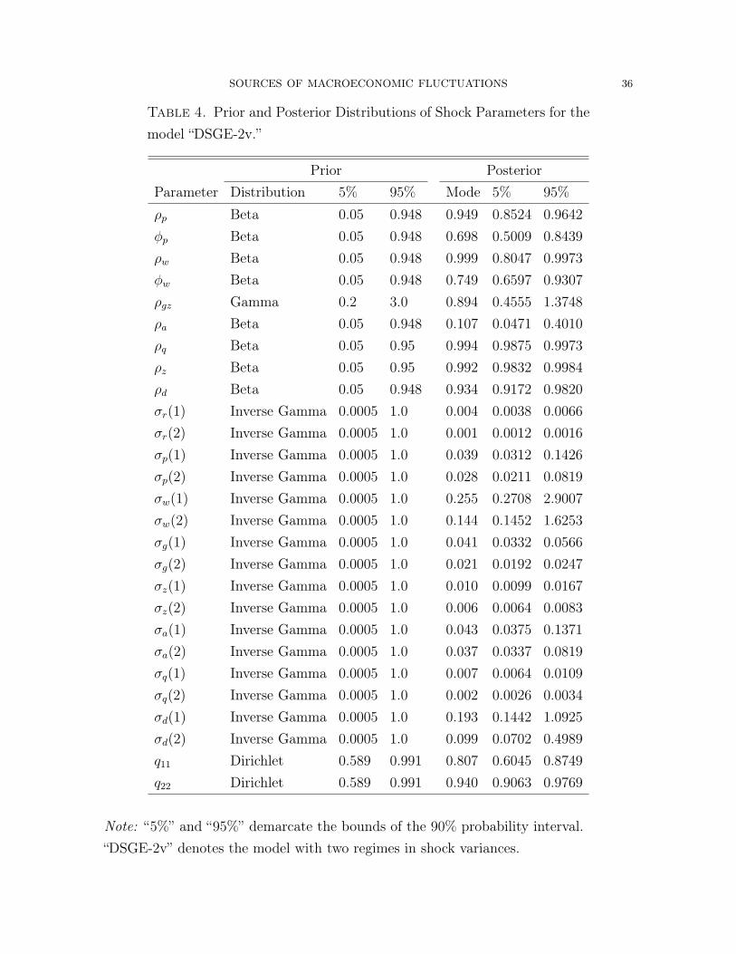
SOURCES OF MACROECONOMIC FLUCTUATIONS 36
Table 4. Prior and Posterior Distributions of Shock Parameters for themodel “DSGE-2v.”
Prior PosteriorParameter Distribution 5% 95% Mode 5% 95%
ρp Beta 0.05 0.948 0.949 0.8524 0.9642
ϕp Beta 0.05 0.948 0.698 0.5009 0.8439
ρw Beta 0.05 0.948 0.999 0.8047 0.9973
ϕw Beta 0.05 0.948 0.749 0.6597 0.9307
ρgz Gamma 0.2 3.0 0.894 0.4555 1.3748
ρa Beta 0.05 0.948 0.107 0.0471 0.4010
ρq Beta 0.05 0.95 0.994 0.9875 0.9973
ρz Beta 0.05 0.95 0.992 0.9832 0.9984
ρd Beta 0.05 0.948 0.934 0.9172 0.9820
σr(1) Inverse Gamma 0.0005 1.0 0.004 0.0038 0.0066
σr(2) Inverse Gamma 0.0005 1.0 0.001 0.0012 0.0016
σp(1) Inverse Gamma 0.0005 1.0 0.039 0.0312 0.1426
σp(2) Inverse Gamma 0.0005 1.0 0.028 0.0211 0.0819
σw(1) Inverse Gamma 0.0005 1.0 0.255 0.2708 2.9007
σw(2) Inverse Gamma 0.0005 1.0 0.144 0.1452 1.6253
σg(1) Inverse Gamma 0.0005 1.0 0.041 0.0332 0.0566
σg(2) Inverse Gamma 0.0005 1.0 0.021 0.0192 0.0247
σz(1) Inverse Gamma 0.0005 1.0 0.010 0.0099 0.0167
σz(2) Inverse Gamma 0.0005 1.0 0.006 0.0064 0.0083
σa(1) Inverse Gamma 0.0005 1.0 0.043 0.0375 0.1371
σa(2) Inverse Gamma 0.0005 1.0 0.037 0.0337 0.0819
σq(1) Inverse Gamma 0.0005 1.0 0.007 0.0064 0.0109
σq(2) Inverse Gamma 0.0005 1.0 0.002 0.0026 0.0034
σd(1) Inverse Gamma 0.0005 1.0 0.193 0.1442 1.0925
σd(2) Inverse Gamma 0.0005 1.0 0.099 0.0702 0.4989
q11 Dirichlet 0.589 0.991 0.807 0.6045 0.8749
q22 Dirichlet 0.589 0.991 0.940 0.9063 0.9769
Note: “5%” and “95%” demarcate the bounds of the 90% probability interval.“DSGE-2v” denotes the model with two regimes in shock variances.
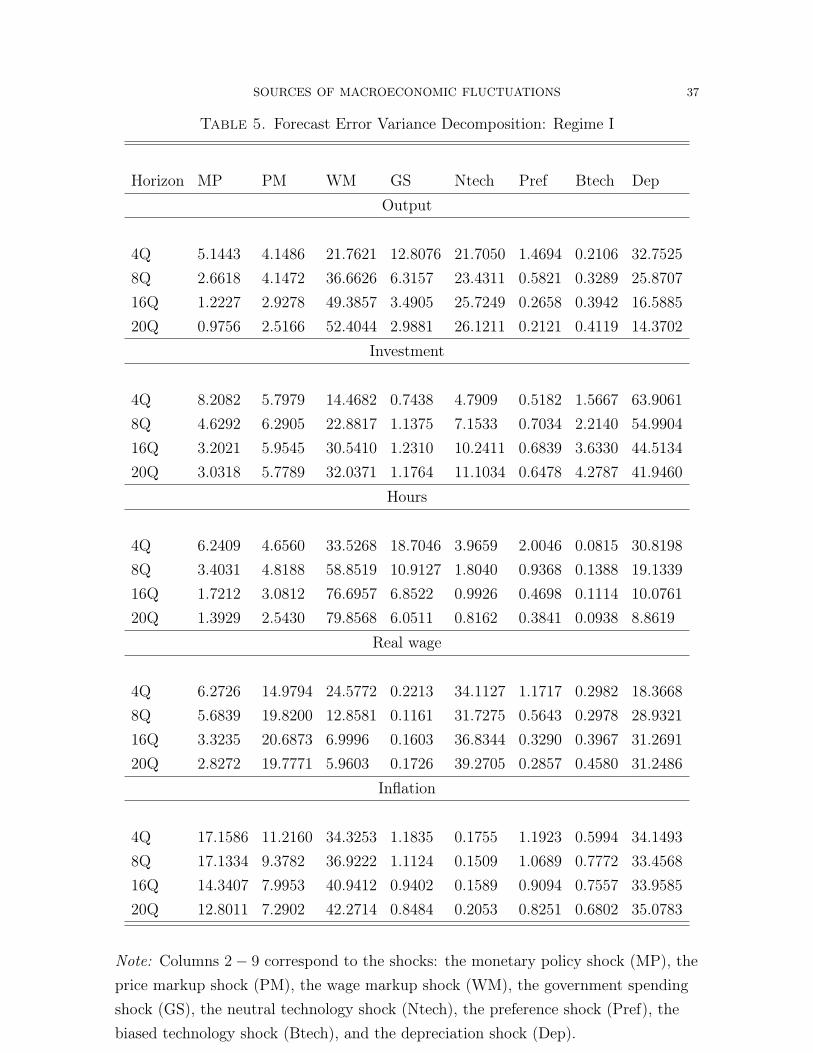
SOURCES OF MACROECONOMIC FLUCTUATIONS 37
Table 5. Forecast Error Variance Decomposition: Regime I
Horizon MP PM WM GS Ntech Pref Btech DepOutput
4Q 5.1443 4.1486 21.7621 12.8076 21.7050 1.4694 0.2106 32.75258Q 2.6618 4.1472 36.6626 6.3157 23.4311 0.5821 0.3289 25.870716Q 1.2227 2.9278 49.3857 3.4905 25.7249 0.2658 0.3942 16.588520Q 0.9756 2.5166 52.4044 2.9881 26.1211 0.2121 0.4119 14.3702
Investment
4Q 8.2082 5.7979 14.4682 0.7438 4.7909 0.5182 1.5667 63.90618Q 4.6292 6.2905 22.8817 1.1375 7.1533 0.7034 2.2140 54.990416Q 3.2021 5.9545 30.5410 1.2310 10.2411 0.6839 3.6330 44.513420Q 3.0318 5.7789 32.0371 1.1764 11.1034 0.6478 4.2787 41.9460
Hours
4Q 6.2409 4.6560 33.5268 18.7046 3.9659 2.0046 0.0815 30.81988Q 3.4031 4.8188 58.8519 10.9127 1.8040 0.9368 0.1388 19.133916Q 1.7212 3.0812 76.6957 6.8522 0.9926 0.4698 0.1114 10.076120Q 1.3929 2.5430 79.8568 6.0511 0.8162 0.3841 0.0938 8.8619
Real wage
4Q 6.2726 14.9794 24.5772 0.2213 34.1127 1.1717 0.2982 18.36688Q 5.6839 19.8200 12.8581 0.1161 31.7275 0.5643 0.2978 28.932116Q 3.3235 20.6873 6.9996 0.1603 36.8344 0.3290 0.3967 31.269120Q 2.8272 19.7771 5.9603 0.1726 39.2705 0.2857 0.4580 31.2486
Inflation
4Q 17.1586 11.2160 34.3253 1.1835 0.1755 1.1923 0.5994 34.14938Q 17.1334 9.3782 36.9222 1.1124 0.1509 1.0689 0.7772 33.456816Q 14.3407 7.9953 40.9412 0.9402 0.1589 0.9094 0.7557 33.958520Q 12.8011 7.2902 42.2714 0.8484 0.2053 0.8251 0.6802 35.0783
Note: Columns 2 − 9 correspond to the shocks: the monetary policy shock (MP), theprice markup shock (PM), the wage markup shock (WM), the government spendingshock (GS), the neutral technology shock (Ntech), the preference shock (Pref), thebiased technology shock (Btech), and the depreciation shock (Dep).

SOURCES OF MACROECONOMIC FLUCTUATIONS 38
Table 6. Forecast Error Variance Decomposition: Regime II
Horizon MP PM WM GS Ntech Pref Btech DepOutput
4Q 1.4623 6.8572 22.2957 10.9572 27.1732 3.5101 0.0921 27.65228Q 0.7325 6.6368 36.3663 5.2312 28.4007 1.3462 0.1392 21.147016Q 0.3285 4.5746 47.8282 2.8228 30.4437 0.6002 0.1629 13.239020Q 0.2611 3.9167 50.5532 2.4070 30.7917 0.4770 0.1696 11.4238
Investment
4Q 2.6142 10.7376 16.6082 0.7130 6.7202 1.3870 0.7675 60.45248Q 1.3975 11.0425 24.8966 1.0335 9.5109 1.7845 1.0280 49.306516Q 0.9411 10.1760 32.3509 1.0888 13.2559 1.6891 1.6423 38.855920Q 0.8887 9.8499 33.8462 1.0379 14.3342 1.5957 1.9291 36.5185
Hours
4Q 1.8550 8.0476 35.9182 16.7333 5.1919 5.0074 0.0373 27.20938Q 0.9744 8.0232 60.7354 9.4043 2.2750 2.2543 0.0611 16.272416Q 0.4847 5.0454 77.8436 5.8075 1.2310 1.1118 0.0482 8.427720Q 0.3918 4.1596 80.9619 5.1229 1.0112 0.9081 0.0406 7.4039
Real wage
4Q 1.5771 21.9006 22.2722 0.1675 37.7754 2.4758 0.1153 13.71618Q 1.4263 28.9214 11.6296 0.0877 35.0659 1.1900 0.1150 21.564116Q 0.8150 29.4979 6.1863 0.1183 39.7808 0.6781 0.1496 22.774020Q 0.6917 28.1379 5.2561 0.1271 42.3184 0.5875 0.1724 22.7089
Inflation
4Q 5.3155 20.2044 38.3260 1.1035 0.2395 3.1041 0.2856 31.42148Q 5.3827 17.1324 41.8078 1.0518 0.2089 2.8220 0.3755 31.218916Q 4.4593 14.4569 45.8850 0.8799 0.2176 2.3764 0.3614 31.363420Q 3.9610 13.1172 47.1437 0.7901 0.2798 2.1456 0.3237 32.2388

SOURCES OF MACROECONOMIC FLUCTUATIONS 39
0
0.2
0.4
0.6
0.8 00.2
0.40.6
0.8
0
500
1000
1500
2000
2500
3000
3500
Average wage markup (µw
−1)Wage stickiness parameter (ξ
w)
Figure 1. The histogram plot for the joint posterior distribution of thewage stickiness parameter and the average wage markup parameter forthe model DSGE-2v.

SOURCES OF MACROECONOMIC FLUCTUATIONS 40
1960 1965 1970 1975 1980 1985 1990 1995 2000 2005 20100
0.1
0.2
0.3
0.4
0.5
0.6
0.7
0.8
0.9
1
Pro
b of
2nd
reg
ime
Figure 2. Posterior probabilities of the second regime for the modelDSGE-2v.

SOURCES OF MACROECONOMIC FLUCTUATIONS 41
0 1 2 3 4 50
0.1
0.2
0.3
Inflation target1 1.5 2 2.5 3
0
0.5
1
1.5
2
Inflation coefficient in Taylor rule
0 0.2 0.4 0.6 0.8 10
1
2
3
4
Price stickness parameter0 0.2 0.4 0.6 0.8
0
1
2
3
4
Wage stickness parameter
2 4 6 8 10 120
0.2
0.4
0.6
0.8
Annual trend growth of investment0 0.2 0.4 0.6 0.8 1
0
0.5
1
1.5
2
Wage indexation
Figure 3. Marginal posterior distributions of some key parameters forthe DSGE-2v model.
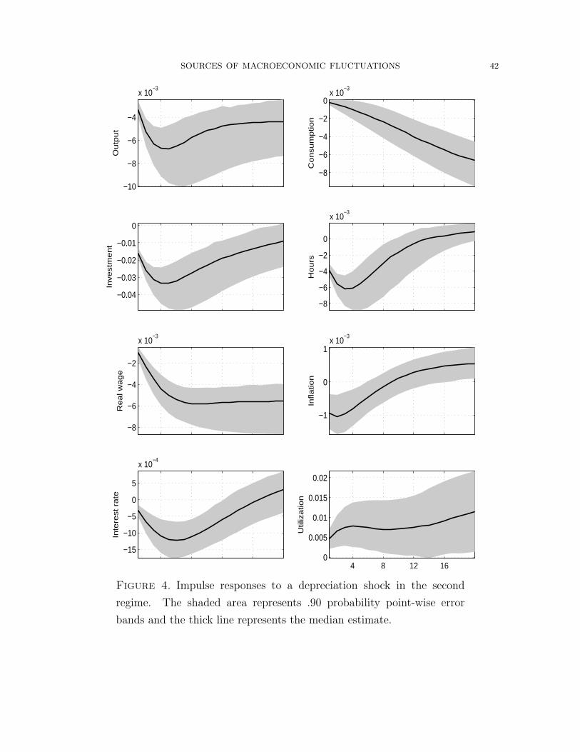
SOURCES OF MACROECONOMIC FLUCTUATIONS 42
−10
−8
−6
−4
x 10−3
Ou
tpu
t
−8
−6
−4
−2
0x 10
−3
Co
nsu
mp
tion
−0.04
−0.03
−0.02
−0.01
0
Inve
stm
en
t
−8
−6
−4
−2
0
x 10−3
Ho
urs
−8
−6
−4
−2
x 10−3
Re
al w
ag
e
−1
0
1x 10
−3
Infla
tion
−15
−10
−5
0
5
x 10−4
Inte
rest
ra
te
4 8 12 160
0.005
0.01
0.015
0.02
Util
iza
tion
Figure 4. Impulse responses to a depreciation shock in the secondregime. The shaded area represents .90 probability point-wise errorbands and the thick line represents the median estimate.

SOURCES OF MACROECONOMIC FLUCTUATIONS 43
−2
0
2
4
6x 10
−4
Ou
tpu
t
−4
−2
0
2
x 10−4
Co
nsu
mp
tion
1
2
3
4
5
x 10−3
Inve
stm
en
t
−2
0
2
4x 10
−4
Ho
urs
1
2
3
4
5
x 10−4
Re
al w
ag
e
0.5
1
1.5
x 10−4
Infla
tion
5
10
15
x 10−5
Inte
rest
ra
te
4 8 12 160.5
1
1.5
2
x 10−3
Util
iza
tion
Figure 5. Impulse responses to an investment-specific technology shockin the second regime. The shaded area represents .90 probability point-wise error bands and the thick line represents the median estimate.

SOURCES OF MACROECONOMIC FLUCTUATIONS 44
4
6
8x 10
−3
Ou
tpu
t
0
2
4
6x 10
−3
Co
nsu
mp
tion
5
10
15
x 10−3
Inve
stm
en
t
−3
−2
−1
0
x 10−3
Ho
urs
5
6
7
8x 10
−3
Re
al w
ag
e
−1
0
1
x 10−4
Infla
tion
−1
0
1
x 10−4
Inte
rest
ra
te
4 8 12 16
0.005
0.01
0.015
0.02
Util
iza
tion
Figure 6. Impulse responses to a neutral technology shock in the sec-ond regime. The shaded area represents .90 probability point-wise errorbands and the thick line represents the median estimate.

SOURCES OF MACROECONOMIC FLUCTUATIONS 45
−10
−8
−6
−4
−2
x 10−3
Ou
tpu
t
−12
−10
−8
−6
−4
−2
x 10−3
Co
nsu
mp
tion
−0.03
−0.02
−0.01
Inve
stm
en
t
−12
−10
−8
−6
−4
−2
x 10−3
Ho
urs
0
2
4
6
x 10−3
Re
al w
ag
e
5
10
15x 10
−4
Infla
tion
2
4
6
8
10
x 10−4
Inte
rest
ra
te
4 8 12 160
0.01
0.02
0.03
Util
iza
tion
Figure 7. Impulse responses to a wage markup shock in the secondregime. The shaded area represents .90 probability point-wise errorbands and the thick line represents the median estimate.

SOURCES OF MACROECONOMIC FLUCTUATIONS 46
References
Altig, D., L. J. Christiano, M. Eichenbaum, and J. Linde (2004): “Firm-Specific Capital, Nominal Rigidities and the Business Cycle,” Federal Reserve Bankof Cleveland Working Paper 04-16.
Basu, S., and J. G. Fernald (1997): “Returns to Scale in U.S. Production: Esti-mates and Implications,” Journal of Political Economy, 105(2), 249Ű–283.
(2002): “Aggregate Productivity and Aggregate Technology,” European Eco-nomic Review, 46(6), 963–991.
Bianchi, F. (2008): “Regime Switches, Agents’ Beliefs, and Post-World War II U.S.Macroeconomic Dynamics,” Manuscript, Princeton.
Bils, M., and P. J. Klenow (2004): “Some Evidence on the Importance of StickyPrices,” Journal of Political Economy, 112(5), 947–985.
Boivin, J., and M. Giannoni (2006): “Has Monetary Policy Become More Effec-tive?,” Review of Economics and Statistics, 88(3), 445–462.
Boldrin, M., L. J. Christiano, and J. D. Fisher (2001): “Habit Persistence,Asset Returns, and the Business Cycle,” American Economic Review, 91(1), 149–166.
Calvo, G. (1983): “Staggered Prices in a Utility-Maximizing Framework,” Journal ofMonetary Economics, 12, 383–398.
Canova, F., and L. Gambetti (2004): “Bad luck or bad policy? On the timevariations of US monetary policy,” Manuscript, IGIER and Universítá Bocconi.
Chari, V., P. J. Kehoe, and E. R. McGrattan (2000): “Sticky Price Models ofthe Business Cycle: Can the Contract Multiplier Solve the Persistence Problem?,”Econometrica, 68(5), 1151–1180.
Christiano, L., M. Eichenbaum, and C. Evans (2005): “Nominal Rigidities andthe Dynamics Effects of a Shock to Monetary Policy,” Journal of Political Economy,113, 1–45.
Christiano, L. J., M. Eichenbaum, and R. Vigfusson (2003): “What HappensAfter A Technology Shock?,” NBER Working Paper 9819.
Clarida, R., J. Galí, and M. Gertler (2000): “Monetary Policy Rules andMacroeconomic Stability: Evidence and Some Theory,” Quarterly Journal of Eco-nomics, CXV, 147–180.
Cogley, T., and T. J. Sargent (2005): “Drifts and Volatilities: Monetary Policiesand Outcomes in the Post WWII U.S.,” Review of Economic Dynamics, 8, 262–302.
SOURCES OF MACROECONOMIC FLUCTUATIONS 47
Cummins, J. G., and G. L. Violante (2002): “Investment-Specific Technical Changein the United States (1947-2000): Measurement and Macroeconomic Consequences,”Review of Economic Dynamics, 5, 243–284.
Del Negro, M., and F. Schorfheide (2008): “Forming Priors for DSGE Models(and How It Affects the Assessment of Nominal Rigidities),” Manuscript, FederalReserve Bank of New York and University of Pennsylvania.
Del Negro, M., F. Schorfheide, F. Smets, and R. Wouters (2007): “On theFit and Forecasting Performance of New Keynesian Models,” Journal of Businessand Economic Statistics, 25(2), 123–143.
Denton, F. T. (1971): “Adjustment of Monthly or Quarterly Series to Annual Totals:An Approach Based on Quadratic Minimization,” Journal of the American StatisticalAssociation, 66, 99–102.
Erceg, C. J., and A. T. Levin (2003): “Imperfect Credibility andn Inflation Persis-tence,” Journal of Monetary Economics, 50, 915–944.
Farmer, R. E., D. F. Waggoner, and T. Zha (2009): “Understanding Markov-Switching Rational Expectations Models,” Journal of Economic Theory, 144, 1849–1867.
Favero, C. A., and R. Rovelli (2003): “Macroeconomic Stability and the Pref-erences of the Fed: A Formal Analysis, 1961–98,” Journal of Money, Credit, andBanking, 35, 545–556.
Fernandez-Villaverde, J., and J. Rubio-Ramirez (Forthcoming): “EstimatingMacroeconomic Models: A Likelihood Approach,” Review of Economic Studies.
Fisher, J. D. M. (2006): “The Dynamic Effects of Neutral and Investment-SpecificTechnology Shocks,” Journal of Political Economy, 114(3), 413–451.
Francis, N., and V. A. Ramey (2005): “Is the technology-driven real business cyclehypothesis dead? Shocks and aggregate fluctuations revisited,” Journal of MonetaryEconomics, 52, 1379–1399.
Galí, J. (1999): “Technology, employment, and the business cycle: Do technologyshocks explain aggregate fluctuations?,” American Economic Review, 89(1), 249–271.
Gambetti, L., E. Pappa, and F. Canova (2008): “The Structural Dynamics of USOutput and Inflation: What Explains the Changes?,” Journal of Money, Credit, andBanking, 40, 369–388.
Gelfand, A. E., and D. K. Dey (1994): “Bayesian Model Choice: Asymptotics andExact Calculations,” Journal of the Royal Statistical Society (Series B), 56, 501–514.
SOURCES OF MACROECONOMIC FLUCTUATIONS 48
Gertler, M., and N. Kiyotaki (2010): “Financial Intermediation and Credit Pol-icy in Business Cycle Analysis,” Manuscript, New York University and PrincetonUniversity.
Geweke, J. (1999): “Using Simulation Methods for Bayesian Econometric Models:Inference, Development, and Communication,” Econometric Reviews, 18(1), 1–73.
Gordon, R. J. (1990): The Measurement of Durable Goods Prices. University ofChicago Press, Chicago,Illinois.
Greenwood, J., Z. Hercowitz, and P. Krusell (1997): “Long-Run Implicationsof Investment-Specific Technological Change,” American Economic Review, 87, 342–362.
Hall, R. E. (1988): “The Relation between Price and Marginal Cost in U.S. Industry,”Journal of Political Economy, 96, 921–947.
Hamilton, J. D. (1994): Times Series Analysis. Princeton University Press, Prince-ton, NJ.
Huang, K. X., and Z. Liu (2002): “Staggered Price-Setting, Staggered Wage-Setting,and Business Cycle Persistence,” Journal of Monetary Economics, 49(2), 405–433.
Huang, K. X., Z. Liu, and L. Phaneuf (2004): “Why Does the Cyclical Behaviorof Real Wages Change Over Time?,” American Economic Review, 94(4), 836–856.
Ireland, P. N. (2005): “Changes in the Federal Reserve’s Inflation Target: Causesand Consequences,” Manuscript, Boston College.
Justiniano, A., and G. E. Primiceri (2006): “The Time Varying Volatility ofMacroeconomic Fluctuations,” NBER Working Paper No. 12022.
(2008): “The Time Varying Volatility of Macroeconomic Fluctuations,” Amer-ican Economic Review, 98(3), 604–641.
Justiniano, A., G. E. Primiceri, and A. Tambalotti (2008): “Investment Shocksand Business Cycles,” Manuscript, Northwestern University.
Levin, A. T., A. Onatski, J. C. Williams, and N. Williams (2006): “MonetaryPolicy Under Uncertainty in Micro-Founded Macroeconometric Models,” in NBERMacroeconomics Annual 2005., ed. by M. Gertler, and K. Rogoff, pp. 229–287. MITPress, Cambridge, MA.
Liu, Z., and L. Phaneuf (2007): “Technology Shocks and Labor Market Dynamics:Some Evidence and Theory,” Journal of Monetary Economics, 54(8), 2534–2553.
Liu, Z., D. F. Waggoner, and T. Zha (2009): “Asymmetric Expectation Effects ofRegime Shifts in Monetary Policy,” Review of Economic Dynamics, 12(2), 284–303.

SOURCES OF MACROECONOMIC FLUCTUATIONS 49
Lubik, T. A., and F. Schorfheide (2004): “Testing for Indeterminacy: An Appli-cation to U.S. Monetary Policy,” American Economic Review, 94(1), 190–219.
Meng, X.-L., and W. H. Wong (1996): “Simulating Ratios of Normalizing Constantsvia a Simple Identity: A Theoretical Exploration,” Statistica Sinica, 6, 831–860.
Pencavel, J. H. (1986): “The Labor Supply of Men: A Survey,” in Handbook of LaborEconomics, ed. by O. C. Ashenfelter, and R. Layard, pp. 3–102. Elsevier, Amsterdam,North Holland.
Primiceri, G. (2005): “Time Varying Structural Vector Autoregressions and Mone-tary Policy,” Review of Economic Studies, 72, 821–852.
Ramachandran, K., V. Urazov, D. F. Waggoner, and T. Zha (2007): “EcoSys-tem: A Set of Cluster Computing Tools for a Class of Economic Applications,”Manuscript, Computing College at Georgia Institute of Technology.
Rotemberg, J. J., and M. Woodford (1997): “An Optimization-Based Economet-ric Framework for the Evaluation of Monetary Policy,” in NBER MacroeconomicsAnnual, ed. by B. S. Bernanke, and J. J. Rotemberg, pp. 297–346. The MIT Press,Cambridge (MA).
(1999): “The Cyclical Behavior of Prices and Costs,” in Handbook of Macroe-conomics, ed. by J. B. Taylor, and M. Woodford, vol. 1B. Elsevier, Amsterdam.
Rupert, P., R. Rogerson, and R. Wright (2000): “Homework in labor econom-ics: Household production and intertemporal substitution,” Journal of MonetaryEconomics, 46(3), 557–579.
Schorfheide, F. (2005): “Learning and Monetary Policy Shifts,” Review of EconomicDynamics, 8(2), 392–419.
Sims, C. A. (2002): “Solving Linear Rational Expectations Models,” ComputationalEconomics, 20(1), 1–20.
Sims, C. A., D. F. Waggoner, and T. Zha (2008): “Methods for Inferencein Large Multiple-Equation Markov-Switching Models,” Journal of Econometrics,146(2), 255–274.
Sims, C. A., and T. Zha (2006): “Were There Regime Switches in US MonetaryPolicy?,” American Economic Review, 96, 54–81.
Smets, F., and R. Wouters (2007): “Shocks and Frictions in US Business Cycles:A Bayesian DSGE Approach,” American Economic Review, 97, 586–606.
Stock, J. H., and M. W. Watson (2003): “Has the Business Cycles Changed?Evidence and Explanations,” in Monetary Policy and Uncertainty: Adapting to aChanging Economy, pp. 9–56. Federal Reserve Bank of Kansas City, Jackson Hole,

SOURCES OF MACROECONOMIC FLUCTUATIONS 50
Wyoming.Tauchen, G. (1986): “Finite State Markov-Chain Approximations to Univariate and
Vector Autoregressions,” Economics Letters, 20, 177–181.Taylor, J. B. (1999): “Staggered Price and Wage Setting in Macroeconomics,” in
Handbook of Macroeconomics, ed. by J. B. Taylor, and M. Woodford, pp. 1009–1050.Elsevier, Amsterdam, North Holland.
Uhlig, H. (2004): “Do Technology Shocks Lead to a Fall in Total Hours Worked?,”Journal of the European Economic Association, 2(2-3), 361–71.
Woodford, M. (2003): Interest and Prices: Foundations of a Theory of MonetaryPolicy. Princeton University Press, Princeton, New Jersey.
Federal Reserve Bank of San Francisco, Federal Reserve Bank of Atlanta, Fed-
eral Reserve Bank of Atlanta and Emory University