Loughborough UniversityInstitutional Repository

Some implications ofsuperconducting quantum

interference to theapplication of master

equations in engineeringquantum technologies

This item was submitted to Loughborough University's Institutional Repositoryby the/an author.

Citation: DUFFUS, S. ...et al., 2016. Some implications of superconduct-ing quantum interference to the application of master equations in engineeringquantum technologies. Physical Review B - Condensed Matter and MaterialsPhysics, 94, 064518.

Additional Information:

• This paper was accepted for publication in the journal Physical ReviewB - Condensed Matter and Materials Physics and the denitive publishedversion is available at http://dx.doi.org/10.1103/PhysRevB.94.064518

Metadata Record: https://dspace.lboro.ac.uk/2134/22477

Version: Accepted for publication

Publisher: c© American Physical Society

Rights: This work is made available according to the conditions of the CreativeCommons Attribution-NonCommercial-NoDerivatives 4.0 International (CC BY-NC-ND 4.0) licence. Full details of this licence are available at: https://creativecommons.org/licenses/by-nc-nd/4.0/

Please cite the published version.

Some implications of superconducting quantum interference to the application ofmaster equations in engineering quantum technologies

S.N.A. Duffus,1, 2 K.N. Bjergstrom,1, 2 V.M. Dwyer,1, 3 J.H. Samson,1, 2

T.P. Spiller,4 A.M. Zagoskin,2 W.J. Munro,5 Kae Nemoto,6 and M.J. Everitt1, 2, ∗

1Quantum Systems Engineering Research Group, LoughboroughUniversity, Loughborough, Leicestershire LE11 3TU, United Kingdom

2Department of Physics, Loughborough University3The Wolfson School, Loughborough University

4York Centre for Quantum Technologies, Department of Physics,University of York, York, YO10 5DD, United Kingdom5NTT Basic Research Laboratories, NTT Corporation,

3-1 Morinosato-Wakamiya, Atsugi, Kanagawa 243-0198, Japan6National Institute of Informatics, 2-1-2 Hitotsubashi, Chiyoda-ku, Tokyo 101-8430, Japan

(Dated: Friday 29th July, 2016)

In this paper we consider the modelling and simulation of open quantum systems from a deviceengineering perspective. We derive master equations at different levels of approximation for a Super-conducting Quantum Interference Device (SQUID) ring coupled to an ohmic bath. We demonstratethat the master equations we consider produce decoherences that are qualitatively and quantitativlydependent on both the level of approximation and the ring’s external flux bias. We discuss the is-sues raised when seeking to obtain Lindbladian dissipation and show, in this case, that the externalflux (which may be considered to be a control variable in some applications) is not confined to theHamiltonian, as often assumed in quantum control, but also appears in the Lindblad terms.

I. INTRODUCTION

With its ability to provide substantial cost savings andspeed up the exploration of parameter space, modellingand simulation plays a central role in the engineering pro-cess. As Quantum Technologies (QTs) move away fromlaboratory demonstrations and become integrated intoconsumer systems, accurate modelling will become in-creasingly important1–5. Here robust, and generally hier-archical, quantitative simulations will be required whichare capable of accurately and reliably predicting the be-haviour of the system-under-development at different lev-els of abstraction. The ultimate ambition of this ap-proach being to achieve a level of realism that would en-able the sort of zero-prototyping that occurs in the designof Very Large Scale Integrated (VLSI) microelectronicsand which is also now becoming an aim of the automo-tive and other industries. Given the intractability byclassical means of modelling complex quantum systems,it is an open question as to how well and how far thisdesign paradigm can be translated to the engineering ofquantum technologies. Consequently, there is a need toinvestigate the extent to which it is possible to develop ahierarchy of system models that is able to provide, froma design perspective, usefully accurate modelling, simu-lation and figures of merit at the component, device andsystem level.

Before one might consider developing such a systemlevel view, it is also necessary to establish the effective-ness of existing device level models and the degree towhich these might be leveraged for such applications. Ofparticular interest, at this stage, is the quantitative ac-curacy of models of open systems for single quantum ob-jects, such as the case of a classical device acting as the

environment for some quantum component. Ultimatelysuch models will need to include time-varying parameterssuch as in the case, for example, of the feedback and con-trol of a quantum resource. One standard approach, thatmight prove effective in forming part of an engineeringdesign strategy, derives from the application of quantummaster equations, as these provide a generic pathway forthe modelling of a quantum system and its interactionwith the environment. Master equations have become astandard tool in this regard as they promise a means ofextracting system properties from environmental influ-ences. It is a general view that the dynamics described isin good qualitative agreement with the ensemble averageof the system being studied, and that deviations of the-ory from experimental observations can be brought intoacceptable line by fine tuning model parameters, leadingto the conclusion that master equations provide a goodphenomenological approach6–8. The most widely usedmaster equations are memoryless, and take the Lindbladform9–12

dρSdt

= − i

~[HS , ρS ] +

1

2

∑j

[Lj , ρSL

†j ] + [LjρS , L

†j ]

(1)

where ρS is the reduced density operator of the system,HS is the system Hamiltonian and the Lj account for theeffects of the environmental degrees of freedom. Lindbladmaster equations dominate work on open quantum sys-tems as they conserve probability (i.e. Tr [ρS ] = 1) andensure that ρS is at least physically acceptable (i.e. thereare no negative probabilities, etc.). Master equations ofnon-Lindblad form, on the other hand, usually will leadto some situations which are unphysical10–14

In this work we seek to explore how effective the master

2

equation approach might be in engineering superconduct-ing quantum devices, and in particular for the case of theSuperconducting Quantum Interference Device (SQUID)ring (an LC circuit enclosing a Josephson junction weaklink) coupled to a low temperature Ohmic bath, with cut-off frequency Ω. We note that Josephson junction baseddevices are currently of significant technological impor-tance, with applications in quantum computation (e.g.D-Wave, IBM and Google) and metrology. Beyond theirsignificance for emerging quantum technologies, there aretwo further reasons we have chosen to investigate the de-coherence of SQUIDs as an example Josepheson junctiondevice.

First, the contribution to the Hamiltonian of theJosephson junction term brings with it non-trivial math-ematical properties which test the suitability of masterequations to quantitative engineering applications (in-cluding potentially control through the externally appliedflux Φx). Recent work has provided an exact solutionto the similar (but simpler) Quantum Brownian Motion(QBM) problem (in a quadratic well) to all orders of BornApproximation. The solution15,16 displays a logarithmicdependence on Ω which indicates the general result forsuch problems that the limit Ω→∞ does not exist (i.e.Ω is finite) and, additionally, highlights the importance ofparameterising the bath properly. The common practiceof terminating master equations at first order in ω0/Ω

(where ω0 = 1/√LC is a characteristic frequency in the

system) assumes that an expansion to second order willonly produce small corrections.

The second reason for our choice of system is that itallows us to investigate the issues in the standard deriva-tion of the master equation for a SQUID/Ohmic envi-ronment for a hierarchy of models, in which ω0/Ω playsthe role of a small expansion parameter. Thus, firstand second order master equations are obtained, usingwhat might be termed standard techniques, and com-pared through quantities at the steady state, such as pu-rity and screening current. The difficulties in such analy-sis are discussed and the generally bespoke nature of suchmethods highlighted. Finally, while a higher order Bornseries approximation might be more valuable, the issueswhich arise in the current, simpler analysis are quite sig-nificant enough and are likely to be indicative of thoseconsiderations that an investigation of stronger couplingthrough a Born series would require.

II. MODEL - A SQUID WITH A LOSSY BATH

The system considered here consists of a SQUID ringcoupled to an Ohmic bath represented by an infinite num-ber of harmonic oscillators at absolute zero temperature.Ideally, the Hamiltonian for this system should be derivedfrom a full quantum field theoretic description or from ageneral quantum circuit model (see, for example, [17]),and such analysis would certainly be needed for any ap-plication of this method to the engineering of a specific

quantum device, however its inclusion here would com-plicate our presentation and distract from our centraldiscussion of the issues associated with deriving masterequations for superconducting systems. The Hamilto-nian for the system is therefore taken to be of the form,H = HS + HB + HI , which is simply the sum of theHamiltonians of the SQUID HS , the bath HB and theinteraction between them HI , given by:

HS =Q2

2C+

(Φ− Φx

)2

2L− ~ν cos

(2πΦ

Φ0

)

HB =∑n

Q2n

2Cn+

Φ2n

2Ln

HI = −(

Φ− Φx

)∑n

κnΦn

(2)

where Q, Qn, Φ and Φn (n = 1, 2, ...) represent the chargeand flux operators of the system and bath modes respec-

tively, so that[Φ, Q

]=[Φn, Qn

]= i~, Φx is an exter-

nally applied flux, and L,C and the Ln, Cn are the induc-tance and capacitance values in each subsystem. As theHamiltonian has not been derived from a complete cir-cuit model, the parameters must be considered as beingthe effective values that arise through the coupling of thecomponents together - thus for example L and the Ln areeffective inductances. The bath mode coupling strengthκn is related to a system damping rate γ through theexplicit expression of the bath spectral density and cor-relation functions11. We note that, as is usually the casewith this sort of ‘particle confined by a potential’ sys-tem, we have not included any capacitive (momentum)coupling; its inclusion would naturally change the analy-sis which follows.

The SQUID Hamiltonian may be simplified to thatof an unshifted harmonic oscillator plus a perturba-tion term through the unitary translation operator T =

exp(−iQΦx/~

). The system Hamiltonians acting in

the translated (external flux) basis may then be writtenas18–20:

H ′S = T †HS T =Q2

2C+

Φ2

2L− ~ν cos

(2π

Φ0

(Φ + Φx

))H ′B = T †HBT = HB =

∑n

Q2n

2Cn+

Φ2n

2Ln

H ′I = T †HI T = −Φ∑n

κnΦn = −ΦB (3)

where we have introduced B as a shorthand for the bathoperator

∑n κnΦn and will drop the primed notation

from now on. As usual, as long as there is no explicit timedependence in the total Hamiltonian H = HS+HB+HI ,the Schrodinger and the Liouville-von Neumann equa-tions are unaltered by the translation. If the externalflux is time dependent there will arise additional terms

3

in H ′S due to this translation of the form QΦx - howeverthese would be small in the adiabatic limit21.

III. REVIEW OF DERIVING THE GENERALFORM OF THE MASTER EQUATION

The derivation of the master equation can now followstandard textbook methods, we include this discussionfor coherence within the paper, however the reader whois familiar with such material may wish to move forwardto section IV. The dynamics of the system+bath is givenby the Liouville-von Neumann equation:

dρ(t)

dt= − i

~[H, ρ(t)] (4)

As it is not generally possible to solve this equation, ana-lytically or numerically, we derive a master equation thatapproximates the dynamics of the reduced density ma-trix ρS(t) for the SQUID ring. Rotating the system intothe interaction picture, Eq. (4) becomes:

dρ(t)

dt= − i

~

[HI(t), ρ(t)

](5)

where we define A = ei(HS+HB)t/~Ae−i(HS+HB)t/~ as therotated version of an operator A. Integrating Eq. (5)yields:

ρ(t) = ρ(0)− i

~

∫ t

0

ds[HI(s), ρ(s)] (6)

It is usual, at this stage, to apply a set of assumptionswhich are collectively known as the Born-Markov approx-imation. This starts with the assumption that, at sometime in the past which we label t = 0, the bath andsystem were uncorrelated, i.e. in a separable pure state,so that ρ(0) = ρS(0) ⊗ ρB(0) where ρS and ρB are thereduced density matrices for the SQUID ring and bathrespectively. This approximation is generally sound inquantum optics but may not hold so well for condensedmatter systems. It is not clear whether non-Markovianmaster equations will become necessary in such cases,however these bring with them a number of additionalchallenges that are beyond the scope of this work. Fornow we impose the uncorrelated assumption and we jus-tify it as being valid at the point that the superconduct-ing condensate first forms. That is, if the condensationprocess removes any existing correlations between theelectrons and their environment, then this approxima-tion is acceptable and t = 0 is taken to be the time atcondensation.

Substituting the expression for ρ(t) into the Liouville-von Neumann equation in the interaction picture, Eq. (5)gives:

dρ(t)

dt= − i

~[HI(t), ρ(0)]− 1

~2

∫ t

0

ds[HI(t), [HI(s), ρ(s)]]

(7)

If further we apply the standard Markovian restrictionthat the bath is memoryless, it is possible to extend thisto ρ(t) = ρS(t)⊗ ρB(t), although previous studies of fullyquantum mechanical models of electromagnetic fieldswith SQUID rings show that there may be significantback-action between the ring and its environment whichcannot be captured by this approximation19,20,22–24 .However, it does allow for a further assumption that thebath is sufficiently big that the SQUID ring will havea negligible effect on it, so that we may take ρB(t) asapproximately constant.

Such considerations already raise the prospect that theBorn-Markov approximation may be inadequate for theaccurate study of condensed matter systems, limiting theuse of master equations in the modelling and simulationfor quantitive applications as part of an engineering so-lution; at best they may offer only a phenomenologicaltool. Despite these difficulties, such phenomenologicalmodels are important and an investigation of their pre-dictions is still worthwhile and we proceed on that basis.The consequence is that Eq. (7) simplifies to:

dρS(t)

dt⊗ ρB = − i

~[HI(t), ρS(0)⊗ ρB ] (8)

− 1

~2

∫ t

0

ds[HI(t), [HI(s), ρS(s)⊗ ρB ]]

To obtain the master equation for the SQUID ring dy-namics, the environment is traced out to yield:

dρS(t)

dt= − i

~TrB([HI(t), ρS(0)⊗ ρB ]) (9)

− 1

~2

∫ t

0

dsTrB([HI(t), [HI(s), ρS(s)⊗ ρB ]])

For a system, linearly coupled to the environment as here,we assume a Ohmic bath with zero mean so that the firstterm above vanishes to give:

dρS(t)

dt= − 1

~2

∫ t

0

dsTrB([HI(t), [HI(s), ρS(s)⊗ ρB ]])

(10)We note that there is increasing interest on the effect ofnon-linear couplings between systems (such as those witha Kerr type nonlinearity)25,26. In such circumstances, ashere, the approximations used in the standard derivationof the master equation would need to be examined indetail. The Markovian approximation further assumesthat the system is only dependent on its current stateand not on its state at earlier times which allows thereplacement ρS(s) → ρS(t) to be applied. Substitutioninto Eq. (10) then leads to the Redfield equation6:

dρS(t)

dt= − 1

~2

∫ t

0

dsTrB

[HI(t), [HI(s), ρS(t)⊗ ρB ]]

.

The correlations with the system at different times maybe made clearer by the change of variables s = t − τwhere τ is interpreted as the relaxation time for the sys-tem. In the Markovian limit, memory effects must be

4

short lived and the integrand within the dissipator decaysvery quickly for τ much larger than the bath correlationtime. With our previous discussion of the validity of theMarkovian approximation and caveats in mind, the lim-its of integration can therefore be extended to infinity(essentially here this requires t 1/Ω). This change ofvariable, together with interchanging the limits of inte-gration, gives the general form of the master equation inthe interaction picture:

dρS(t)

dt= − 1

~2

∫ ∞0

dτ TrB

[HI(t), [HI(t−τ), ρS(t)⊗ρB ]]

(11)

Finally, rotating these equations back into theSchrodinger picture yields the dynamics for the system’sreduced density matrix as:

dρS(t)

dt= − i

~[HS , ρS(t)] (12)

− 1

~2

∫ ∞0

dτ TrB

[HI ,

[HI(−τ), ρS(t)⊗ ρB

]].

as, for linear coupling and a time-independent Hamilto-

nian, Φ(−τ) = e−iHSτ/~ΦeiHSτ/~ (as Φ commutes with

HI and HB). This equation is of the form of a modi-fied Liouville-von Neumann equation. The first term de-scribes the free evolution of the system while the secondterm, the dissipator, represents non-unitary loss. Notethat rotation to and from the interaction picture will besignificantly more complex with a time-dependent exter-nal flux, or if the device dynamics includes a time-varyingcontroller.

Using the SQUID-environment interaction Hamilto-nian above, and expanding the commutators within theintegral, this can be written in the form:

dρS(t)

dt= − i

~[HS , ρS(t)]

+1

~2

∫ ∞0

dτ( i

2D(−τ)[Φ, Φ(−τ), ρS(t)]

−1

2D1(−τ)[Φ, [Φ(−τ), ρS(t)]]

)(13)

Here ρS(t) describes the reduced density matrix in theexternal flux basis and [·] and · denote commutatorsand anticommtutators respectively. As the terms in theintegrand of Eq. (13) are both commutators, the cyclicproperty of Tr ensures that Tr(dρ/dt) = 0, thus Tr(ρ) = 1for all t. However Lindblad form is not assured. Thefunctions D and D1 are related to the bath correlationfunction B by11:

D1(−τ) + iD(−τ) = 2 〈BB(−τ)〉B (14)

where the expectation value with respect to the bath isgiven by 〈BB(−τ)〉B = TrBBB(−τ)ρB. In this case,the coupling constants, κn, in Eq. (2) are determined by

a quasi-continuous spectral density J(ω), which describesthe absorption and emission of energy arising from thecoupling to the environment. The dissipation and noisekernels can be written in terms of the spectral densityas11:

D(−τ) = 2~∫ ∞

0

dωJ(ω) sin (ωτ)

D1(−τ) = 2~∫ ∞

0

dωJ(ω) coth

(~ω

2kBT

)cos (ωτ)

(15)

Whilst the first expression is easy to evalutate for anOhmic bath, the second requires the separation intoslowly and rapidly oscillating terms, as indicated in [14],which enables us to write D1(−τ) as approximately:

D1(−τ) =ω0

2coth

(~ω0

2kBT

)∫ ∞0

dωJ(ω)

ωcos (ωτ) (16)

For an Ohmic bath with a Lorentz-Drude cutoff function,with cutoff frequency Ω, the spectral density is given by:

J(ω) =2Cγ

πω

Ω2

Ω2 + ω2(17)

where ω is a bath frequency and γ represents the dampingrate of the system.

In this case, the dissipation11 and noise14 kernels,D(−τ) and D1(−τ), may be written, respectively, as:

D(−τ) = 2Cγ~Ω2e−Ω|τ | sgn τ

D1(−τ) = C~γΩω0 coth

(~ω0

4kBT

)e−Ω|τ |

in the mid-low temperature regime11,14, for system ther-mal energy kBT . In the limit temperature T → 0 thenoise kernel reduces further to

D1(−τ) = C~γΩω0e−Ω|τ | (18)

The approximation used in Eq. (16) has an easier justi-fication at higher temperatures. At low temperatures itwould be more accurate to swap the order of the time in-tegral in Eq. (13) and the frequency integral in Eq. (15),as is done for the special case of the Quantum BrownianMotion10–12,15,16,27–33. Details of this will be presentedin a future work.

IV. INTEGRATING THE MASTER EQUATION

An issue which arises with QBM is a logarithmic cut-offdivergence (leading to a log(Ω) dependence in the diffu-sion terms) in the exact solution of the master equation,thus making the large Ω limit difficult. Most approxi-mations stop at first order in ω0/Ω, before the log-termenters, and this rather begs the question of how accuratethis is and consequently we seek here both first and sec-ond order solutions. To derive a useful master equation

5

it is necessary to evaluate, or at least approximate, thedissipator integral in (13). A common means of approx-

imating the relaxation-time dependent flux term Φ(−τ)is through a power series expansion in τ , such that:

Φ(−τ) =∑n

An[Φ]τn (19)

where the functional An[Φ] is found by equating pow-ers of τ from the Baker-Campbell-Hausdorff expansion

of Φ(−τ) = e−iHSτ/~ΦeiHSτ/~ i.e.:

Φ(−τ) = Φ + τ

[− iHS

~, Φ

]+τ2

2!

[− iHS

~,

[− iHS

~, Φ

]]

+ · · ·+ τn

n!

[− iHS

~, ...,

[− iHS

~, Φ

]](20)

For the simpler case of a quantum Brownian particle ina harmonic oscillator potential, each of the An[Φ] is pro-portional to either the position or momentum operator,with pre-factors which add to give trigonometric terms16.Unfortunately the same cannot be said for the SQUID.Due to the nonlinear nature of the Josephson junctionterm in the Hamiltonian, the series grows in complexityas the order is increased. For this reason it is not possi-ble to evaluate Φ(−τ) analytically and it is necessary totruncate the series in Eq. (19). Analysis of this seriesshows it to be convergent and a more detailed study willfollow in later work. Including more terms in the seriesthough should lead to increasingly accurate master equa-tions and here we explore the impact of truncating to firstand second order. Note that if the system Hamiltonianwere to be time dependent (possess a time dependent ex-ternal flux Φx(t)), the series would grow significantly incomplexity and this method may not be applicable.

Substituting Eq. (19) into the expressions for the dis-sipator of Eq. (13) yields the non-Lindblad master equa-tion:

dρS(t)

dt= − i

~[HS , ρS(t)] +

iCγΩ

~

[Φ,

∑n

n!

ΩnAn[Φ], ρS(t)

]− C~γω0

2~

[Φ,

[∑n

n!

ΩnAn[Φ], ρS(t)

]](21)

where the identities for the dissipation and noise terms:

i

2~2

∫ ∞0

dτD(−τ)Φ(−τ) =∑n

iCγΩ

~n!

ΩnAn[Φ]

− 1

2~2

∫ ∞0

dτD1(−τ)Φ(−τ) = −C~γω0

2~∑n

n!

ΩnAn[Φ]

(22)

have been used alongside the identityΩn+1

∫∞0

dττne−Ωτ = n!.

V. FIRST ORDER MASTER EQUATION

If the series of Eq. (19) is truncated to first order inτ then the summations in Eq. (21) can be simplified ac-cordingly:

∑n

n!

ΩnAn ≈ A0 +

1

ΩA1 = Φ− Q

ΩC(23)

so that Eq. (21) yields the first order master equation:

dρSdt

=− i

~[HS , ρS ] +

renormalises L︷ ︸︸ ︷iCγΩ

~[Φ2, ρS ]−

dissipation term︷ ︸︸ ︷iγ

~[Φ, Q, ρS]

− Cω0γ

2~

([Φ, [Φ, ρS ]]︸ ︷︷ ︸noise term

− 1

ΩC[Φ, [Q, ρS ]]︸ ︷︷ ︸

first order cutoff

)(24)

It is worth remarking, at this stage, that additional ca-pacitive coupling in the interaction Hamiltonian (Eq. 2)will lead to a much more complicated expression thanEq. (24) due the the presence of a commutation relationbetween the charge operator and the Josephson couplingenergy and would inevitably lead to a non-linear depen-dence on external flux even in a first order master equa-tion. We believe this would produce noticeable differ-

6

ences in theory which could be observed experimentallyeven for modest couplings (again a more detailed studywill be the subject of future work). The final term in eqn(25) vanishes in the limit of high cutoff frequency. Thislimit is often assumed in quantum optics and the termneglected but, as indicated above, is not be applicableto condensed matter systems and we retain it for thisreason, and because it is also a necessary ingredient forturning Eq. (24) into Lindblad form.

The second term in Eq. (24) is simply a renormalisa-tion of the potential, or more specifically a shift in theSQUID inductance34–36 by a factor of λ = 2Ωγ

ω20(1+2Ωγ/ω2

0)

and can therefore be absorbed into the free evolution partof the equation to give:

dρ

dt=− i

~[HS1 , ρ]− iγ

~[Φ, Q, ρ]

− Cω0γ

2~

([Φ, [Φ, ρ]]− 1

ΩC[Φ, [Q, ρ]]

) (25)

where HS1 is of exactly the same form as HS as in Eq. (3)but uses the bare inductance of the SQUID ring, sinceL0 = L/(1 − λ), instead of L. Eq. (25) is a Caldeira-Leggett equation27, rather than in the Lindblad formof Eq. (1), and thus does not ensure all solutions will bephysically sensible13 (i.e. a density operator that is pos-tive). The simplest way to address this issue is to trans-form Eq. (25) into Lindblad form, as for QBM11,14,37.This is achieved through the addition of a term propor-tional to [Q, [Q, ρ]] . The physical significance of thisaddition becomes clear when considering the same sys-tem capacitively (rather than inductively) coupled to thebath, when such a term arises naturally. One can thenthink of this addition as the inclusion of a capacitiveelement in the interaction, an effect that will be pre-sented in future work. It should be noted that unlike thecase of QBM at high temperatures, the additional term isnot necessarily small. Nevertheless, proceeding this wayleads to

dρ

dt= − i

~[H, ρ] +

1

2

([L, ρL†] + [Lρ, L†]

)H = HS1

+~γ2

(XP + P X

)L = γ

12

[X +

(i− ξ

2

)P

] (26)

where we have introduced the dimensionless quantities

X =√

Cω0

~ Φ, P =√

1C~ω0

Q and ξ = ω0/Ω. There

are a number of observations to be made here in rela-tion to the introduction of the [Q, [Q, ρ]] into Eq. (25).First Eq. (26) recovers, in the limit ξ → 0, a more famil-iar Lindblad proportional to the annihilation operator.What the derivation here demonstrates is that in assum-ing L =

√2γa, for some γ, a significant adjustment to

the master equation is being made. Second, it is clearthat, within the Hamiltonian H, there exists a squeezingterm, which cannot be included in the Lindblad terms,

but which may instead be included in the system Hamil-tonian. This arises as a corollary of applying the Lind-blad process and its inclusion is very often neglected inthe literature. However, it is a necessary part of the sys-tem evolution which provides a physical frequency shift,and is essential in recovering the quantum to classicaltransition38–42.

This is evident from the harmonic oscillator com-ponent of the SQUID ring Hamiltonian, H =

HS1+ (~γ)/2

(XP + P X

)= ~ω(a†a + 1/2) +

(~γi)/2(a†2 − a2

); the significance of the second (the

squeezing) term appears when considering the correspon-dence limit. If the quantity Tr

(ddt (ρa)

)is found from

Eq. (1), without the squeezing term, one obtains an ex-pression for the expectation value of the evolution of theposition operator:

〈x(t)〉 =(〈x+〉 eiωt + 〈x−〉 e−iωt

)e−γt (27)

which describes a system oscillating at a frequency ω anddecaying at a rate e−γt.

Although there appears to be agreement with decayrate in classical models for the damped harmonic oscilla-tor, frequency shifts are not accounted for; and this vio-lates the correspondence principle. This result suggeststwo things: Lindblad operators describe dissipation only,and the frequency shift is described by the additionalHamiltonian term. The impact of the squeezing termcan be seen by performing a Bogoliubov transform43 sothat the Hamiltonian may be written in terms of a new

set of raising and lowering operators, b† and b

b = ua+ va†

b† = u∗a† + v∗a

that reproduce a† and a in the limit where γ → 0. Sat-isfying the requirement that |u|2 + |v|2 = 1 through theassumption that the constants u = sec θ and v = i tan θ,allows the Hamiltonian to be rewritten as

H ′ = ~ωb†b = ~ω√

1− γ2

ω2b†b

It is clear to see that this term is responsible for thefrequency shift of the dissipating system.

The Lindblad in Eq. (26) is a function of cut-off fre-quency as ξ = ω0/Ω, we now establish how significantthis is when compared with simply assuming a Lindbladterm proportional to the annihilation operator. Thereare many ways that we can quantify the effect of chang-ing cut-off frequency, but as our focus in this work is onestimating the effects of environmental decoherence wechoose to compare the purity, Tr

[ρ2], of the steady state

solution to Eq. (26) as a function of external flux andcut-off frequency. This is shown in Fig. 1. We first notethat in the limit Ω → ∞ we have ξ → 0 and the Lind-blad reduces to the annihilation operator times

√2γ and

the standard form of the master equation that has beenapplied to SQUIDs in previous work44–48.

7

2P

urity

, Tr[½

]

External flux, Φ /Φ x 0

0.4

0.5

0.6

0.7

0.8

0.9

1

0 0.2 0.4 0.6 0.8 1

0.45 0.55

First OrderΩ=20!0

First OrderΩ=10!0

First OrderΩ=2!0

AnnihilationOperator

FIG. 1. (colour online) To quantify the importance of cutofffrequency, Ω, in the first order master equation Eq. (26), we

show Tr[ρ2]

as a function of external flux Φx for the steadystate solution to the master equation for ξ = ω0/Ω equal to0 (Ω = ∞), 0.05 (Ω = 20ω0), 0.1 (Ω = 10ω0) and 0.5 (Ω =2ω0). We see that Ω =∞ and Ω = 20ω0 are indestinguishablewhilst near the dip at Φx = 0.5Φ0 there are small differencesat Ω = 10ω0. While the functional form is similar the effectof cut-off frequency is significant for Ω = 2ω0. Note, circuitparameters are C = 5 × 10−15F, L = 3 × 10−10H and Ic ≈3µA. The sharp dip at Φx = Φ0/2 is due to the fact thatthe SQUID’s potential becomes a double well and the groundenergy eignstate is a Schrodinger cat (i.e. a macroscopicallydistinct superposition of states). Decoherence of this stateproduces a statistical mixture of states equally localised ineach well - as there is a 50% chance of being in either wellTr[ρ2]

= 0.5 at Φx = Φ0/2. As we move away from thisbias point the ground state rapidly loses its Schrodinger catstructure and so decoherence is less significant at these values.The width of this dip is related to the the barrier hight andcan be changed by altering circuit parameters.

In this work, we have chosen reasonable SQUID pa-

rameters values of C = 5× 10−15F and L = 3× 10−10Hare used in all caluculations together with a Josephsoncoupling energy20 of ~ν = IcΦ0/2π = 9.99 × 10−22J,where Φ0 = h/2e is the flux quantum and Ic is the criti-cal current of the weak link (here Ic ≈ 3µA). The exter-nal environment is defined by the parameters γ, Ω, ~ν,and Φx where the damping rate γ determines the rate ofloss in the system. Treating the environment as a cavityof harmonic oscillator modes, this loss is directly pro-portional to the cavity quality factor Qc = 2πωc/γ forcavity frequency ωc. This quality factor can range fromQc ∼ 102 to Qc ∼ 106 or higher49,50. The cutoff fre-quency, Ω, defines the peak frequency of the bath’s spec-tral density which has a similar form to the impedancein Josephson circuits51,52. The results shown in Fig. 1might lead us to conclude that for a cut off frequency ofΩ = 10ω0 (ξ = 0.1) and higher (lower) that the usualchoice of a Lindblad proportional to the annihilation op-erator is a good one. In the next section we show thatthis conclusion is incorrect.

VI. SECOND ORDER APPROXIMATION

Although for systems of this type it is often assumed tobe adequate, truncation at first order of series (Eq. (23))may not always suffice and higher order terms in τ (orequivalently ω0/Ω) may be important; consideration ofa second order expression will help to justify that. Itis also important to explore the impact of higher orderterms as higher order models may differ quantitatively,if not qualitatively, to the first order model. ExpandingEq. (23) to second order in τ we obtain:

∑n

n!

ΩnAn ≈ Φ− Q

ΩC−ω

2

Ω2

(Φ +

2π~νLΦ0

sin

(2π

Φ0(Φ + Φx)

))(28)

where the external flux dependence, originating from thenon-linear SQUID potential, can be seen to enter thedissipator for the first time. Substituting (28) into (22)then allows (13) to be rewritten as:

dρSdt

= − i

~[HS , ρS(t)] +

iγΩC

~

( renormalises L︷ ︸︸ ︷(1− ω2

0

Ω2

)[Φ2, ρS(t)]]−

1st order dissipation︷ ︸︸ ︷1

ΩC[Φ, Q, ρS(t)]−

2nd order dissipation︷ ︸︸ ︷2π~νL

Φ0

ω20

Ω2

[Φ,

sin

(2π

Φ0(Φ + Φx)

), ρS(t)

])

− γω0C

2~

((1− ω2

0

Ω2

)[Φ, [Φ, ρS(t)]]︸ ︷︷ ︸

1st and 2nd order noise

− 1

ΩC[Φ, [Q, ρS(t)]]︸ ︷︷ ︸

1st order in cutoff

− 2π~νLΦ0

ω20

Ω2

[Φ,

[sin

(2π

Φ0(Φ + Φx)

), ρS(t)

]]︸ ︷︷ ︸

2nd order cutoff

)

(29)

where once again HS consists of the true in-ductance of the SQUID ring after second or-der renormalisation is accounted for, i.e. λ =

(2γΩ

(1− ω2

0

Ω2

))/ω2

0

(1 + 2γΩ

ω20

(1− ω2

0

Ω2

)).

Eq. (29) is once again not of Lindblad form, and suffersfrom the associated problems. However it may be madeso by following the same process as in the first order case,

8

External flux, Φ /Φ x 0

³ at Δ

min

0.6

0.65

0.7

0.75

0.8

0.85

0.9

0.95

1

0 0.2 0.4 0.6 0.8 1

Ω=50!0

Ω=10!0

Ω=2!0

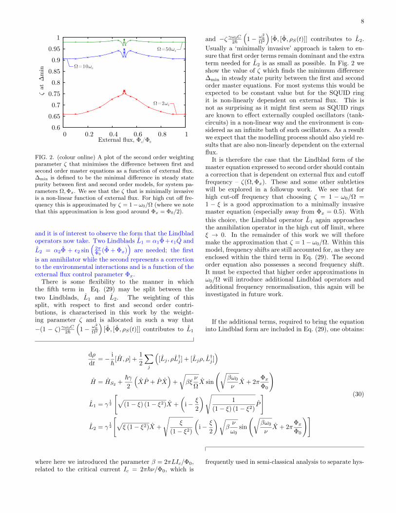
FIG. 2. (colour online) A plot of the second order weightingparameter ζ that minimises the difference between first andsecond order master equations as a function of external flux.∆min is defined to be the minimal difference in steady statepurity between first and second order models, for system pa-rameters Ω,Φx. We see that the ζ that is minimally invasiveis a non-linear function of external flux. For high cut off fre-quency this is approximated by ζ = 1−ω0/Ω (where we notethat this approximation is less good around Φx = Φ0/2).

and it is of interest to observe the form that the Lindbladoperators now take. Two Lindblads L1 = α1Φ+ ε1Q and

L2 = α2Φ + ε2 sin(

2πΦ0

(Φ + Φx))

are needed; the first

is an annihilator while the second represents a correctionto the environmental interactions and is a function of theexternal flux control parameter Φx.

There is some flexibility to the manner in whichthe fifth term in Eq. (29) may be split between the

two Lindblads, L1 and L2. The weighting of thissplit, with respect to first and second order contri-butions, is characterised in this work by the weight-ing parameter ζ and is allocated in such a way that

−(1 − ζ)γω0C2~

(1− ω2

0

Ω2

)[Φ, [Φ, ρS(t)]] contributes to L1

and −ζ γω0C2~

(1− ω2

0

Ω2

)[Φ, [Φ, ρS(t)]] contributes to L2.

Usually a ‘minimally invasive’ approach is taken to en-sure that first order terms remain dominant and the extraterm needed for L2 is as small as possible. In Fig. 2 weshow the value of ζ which finds the minimum difference∆min in steady state purity between the first and secondorder master equations. For most systems this would beexpected to be constant value but for the SQUID ringit is non-linearly dependent on external flux. This isnot as surprising as it might first seem as SQUID ringsare known to effect externally coupled oscillators (tank-circuits) in a non-linear way and the environment is con-sidered as an infinite bath of such oscillators. As a resultwe expect that the modelling process should also yield re-sults that are also non-linearly dependent on the externalflux.

It is therefore the case that the Lindblad form of themaster equation expressed to second order should containa correction that is dependent on external flux and cutofffrequency – ζ(Ω,Φx). These and some other subtletieswill be explored in a followup work. We see that forhigh cut-off frequency that choosing ζ = 1 − ω0/Ω =1 − ξ is a good approximation to a minimally invasivemaster equation (especially away from Φx = 0.5). With

this choice, the Lindblad operator L1 again approachesthe annihilation operator in the high cut off limit, whereξ → 0. In the remainder of this work we will theforemake the approximation that ζ = 1−ω0/Ω. Within thismodel, frequency shifts are still accounted for, as they areenclosed within the third term in Eq. (29). The secondorder equation also possesses a second frequency shift.It must be expected that higher order approximations inω0/Ω will introduce additional Lindblad operators andadditional frequency renormalisation, this again will beinvestigated in future work.

If the additional terms, required to bring the equationinto Lindblad form are included in Eq. (29), one obtains:

dρ

dt= − i

~[H, ρ] +

1

2

∑j

([Lj , ρL

†j ] + [Ljρ, L

†j ])

H = HS2+

~γ2

(XP + P X

)+

√βξ

ν

ΩX sin

(√βω0

νX + 2π

ΦxΦ0

)

L1 = γ12

[√(1− ξ) (1− ξ2)X +

(i− ξ

2

)√1

(1− ξ) (1− ξ2)P

]

L2 = γ12

[√ξ (1− ξ2)X +

√ξ

(1− ξ2)

(i− ξ

2

)√βν

ω0sin

(√βω0

νX + 2π

ΦxΦ0

)](30)

where here we introduced the parameter β = 2πLIc/Φ0,related to the critical current Ic = 2π~ν/Φ0, which is

frequently used in semi-classical analysis to separate hys-

9

0.4

0.5

0.6

0.7

0.8

0.9

1

0 0.2 0.4 0.6 0.8 1

s t1 OrderΩ=10!0

nd2 OrderΩ=10!0

s t1 OrderΩ=2!0

2P

urity

, Tr[½

]

External flux, Φ /Φ x 0

FIG. 3. (colour online) The purity Trρ2(t) of the steadystate solutions of the first order, Eq. (26), and second or-der Eq. (30), Lindblad master equations. In this figure we seeevidence that the order of truncation has a bigger effect onthe steady state purity than one might expect when comparedto that of decreasing cut-off frequency.

teretic (β > 1) from non-hysteretic behaviour (β ≤ 1).

In Fig. 3 we compare the purity Trρ2(t) of the steadystate solutions of the first order, Eq. (26), and second or-der Eq. (30), Linblad master equations for a cut-off fre-quency of Ω = 10ω0. We have also included for compari-son the first order master equation steady state purity forΩ = 2ω0. In Fig. 1, for a cut-off frequency of Ω = 10ω0,we concluded that there was little difference between thesteady state solution to the first order corrected mas-ter equation and one that just assumed an annihilationoperator as a Lindblad. In Fig. 3, for the same value ofcut-off frequency, we observe that the steady state purityis much lower and changes slightly in functional form inthe second order model. This indicates that neither theannihilation operator nor first order Lindblads are suffi-cient to quantitatively model the effects of decoherenceon the SQUID ring.

The difference between first and second order modelsis less obvious when considering the expectation valueof observables, such as screening current, as shown inFig. 4. This suggests that device characterisation basedsolely on simple expectation values of observables such aflux may not be sufficient and a more rigorous analysisof decoherence times, T1 and T2, as functions of externalflux is necessary in order to produce a good phenomenol-ogy. Such an approach may be used to parameterise themaster equation framework presented in this work and toassess its effectiveness in modelling decoherence processeson Josephson junction based devices.

-2

-1.5

-1

-0.5

0

0.5

1

1.5

2

0 0.2 0.4 0.6 0.8 1

0.45 0.55

External flux, Φ /Φ x 0

Scre

enin

g C

urre

nt (¹A

)

s t1 OrderΩ=10!0

nd2 OrderΩ=10!0

FIG. 4. (colour online) A plot of the expectation value of

screening current,⟨

Φ/L⟩

as a function of external flux for

first order (red) and second order (blue) models at a bath cut-off frequency of Ω = 10ω0. Despite the two models differingquite largely in terms of steady state purity, the expectationvalues of observables remain very similar.

VII. CONCLUSIONS

The necessity to consider stronger environmental cou-pling than might be admitted in lowest order Born Ap-proximation, or the effects of a finite bath cut-off fre-quency, or of a device operating at low temperature, sug-gest that the standard Born-Markov development of aMaster Equation will need to be extended. The mostobvious way to do this is through a small parameter ex-pansion, such as the Born series or, as here, by extendingthe large cut-off limit by developing the model as a seriesin the small parameter ω0/Ω, or similarly by extendinga zero temperature limit. We have chosen, here, perhapsthe simplest case (that of a finite cut-off), in the certainknowledge that whatever difficulties one finds are verylikely to appear in all others such attempts.

The most obvious consequence of the present anay-sis is that the correction obtained by including secondorder terms (in ω0/Ω) in the Master Equation is notan insignificant one, leading to steady-state impurities1−P (ρ) which are twice those predicted by using a firstorder model. More subtle is the appearance of the ex-ternal flux Φx entering the Master Equation, not onlyin the Hamiltonian terms, but also in the second orderLindblad. Indeed with capacitive coupling the externalflux is likely to appear in Lindblads at all orders. Asthe Josephson coupling energy dictates the height of thepotential well, and therefore the tunnelling probability,SQUIDs are (notoriously) sensitive to external magneticfields and so it is reasonable to expect a strong externalflux dependence19,20,53; Eq. (30) shows such a depen-dence lies also within the dissipator. Although this islargely contrary to the assumptions of quantum control,where it is generally considered to be the case that, for

10

systems with Lindbladian dissipation, control parameterssuch as Φx will only enter through the Hamiltonian (see,e.g., [54]), it is evident from the form of Eq. 21 that Φxcan play an important role in dissipation. That the dissi-pator will in general a function of control parameters hasbeen pointed out previously55, the current analysis showsthey may not all enter at the same order. Furthermore,we have shown that the second order correction to themaster equation has a surprisingly large effect. Hence,an understanding of this phenomenon and the role ofΦx will be of importance to those working on Josephsonjunction based devices especially for emerging quantumtechnologies.

Recent analysis of the Quantum Brownian Motion(QBM) system indicates that both regular and anoma-lous diffusion parameters show a logarithmic divergenceon bath cut-off frequency Ω, implying a finite cut-off. Itthus makes sense to consider a series solution, to differ-ent orders of ω0/Ω, if only to check that the common firstorder truncation is accurate. It is not surprising that, aswith QBM, it is necessary to add extra terms in orderto bring the master equation into Lindblad form and soavoid unphysical system development. However, in oursecond order approximation, the extra term needed tocomplete the first order Lindblad L1 is of a lower order

than the terms which make up the second order Lind-blad L2. This makes the ‘minimally invasive’ argumenta difficult one to sustain and so we appear to be left withthe choice of abandoning hierarchical checks, reworking anew standard method, or abandoning the Lindblad formfor systems such as these. None of which is attractive.

With the exception of a quadratic constraining poten-tial, which is simple because the position operator (Φhere) links only neighbouring states of fixed energy dif-ference ω0, all other systems are likely to run into thesame difficulties we have here.

ACKNOWLEDGMENTS

MJE would like to thank Kae Nemoto and SNADwould like to thank Todd Tilma for the generous hos-pitality, valuable discussions, and support whilst visitingthem in Tokyo. SNAD and MJE would like to thankMichael Hanks and Jason Ralph for many valuable, andenjoyable, discussions. MJE, KNB and VMD would liketo thank the DSTL for their support through the grantEngineering for Quantum Reliability. This paper recog-nises the use of the ‘Hydra’ High Performance System atLoughborough University.

∗ m.j.everitt@lboro.ac.uk1 J. P. Dowling and G. J. Milburn, Philosophical transac-

tions. Series A, Mathematical, physical, and engineeringsciences 361, 1655 (2003).

2 S. Boixo, T. F. Rønnow, S. V. Isakov, Z. Wang, D. Wecker,D. a. Lidar, J. M. Martinis, and M. Troyer, Nature Physics10, 218 (2014).

3 J. Clarke and I. Braginski, Alex, eds., The SQUID Hand-book , Vol. 1 (Wiley-VCH, 2004) pp. 127–170.

4 B. Ruggiero, V. Corato, C. Granata, L. Longobardi,S. Rombetto, and P. Silvestrini, Physical Review B 67,132504 (2003).

5 K. Ogunyanda, W. Fritz, and R. van Zyl, Journal of En-gineering, Design and Technology 13, 298 (2015).

6 U. Weiss, Quantum Dissipative Systems (World ScientificPublishing, 1999).

7 E. Joos, H. D. Zeh, C. Kiefer, D. Guilini, J. Kupsch, andO. Stamatescu, I, Decoherence and the Appearance of aClassical World in Quantum Theory , 2nd ed. (Springer,2003).

8 J. P. Santos and F. L. Semiao, Physical Review A - Atomic,Molecular, and Optical Physics 89, 022128 (2014).

9 G. Lindblad, Communications in Mathematical Physics48, 119 (1976).

10 C. W. Gardiner, Quantum Noise (Springer-Verlag, Berlin,1991).

11 H. Breuer and F. Petruccione, The Theory of Open Quan-tum Systems (Oxford University Press, 2002).

12 M. Schlosshauer, Decoherence: And the Quantum-To-Classical Transition (Springer, 2007).

13 W. Munro and C. Gardiner, Physical Review A 53, 2633(1996).

14 S. Gao, Physical Review Letters 79, 3101 (1997).15 C. H. Fleming, A. Roura, and B. L. Hu, Annals of Physics

326, 1207 (2011).16 P. Massignan, A. Lampo, J. Wehr, and M. Lewenstein,

Physical Review A - Atomic, Molecular, and OpticalPhysics 91, 033627 (2015).

17 G. Burkard, Physical Review B - Condensed Matter andMaterials Physics 71, 1 (2005).

18 C. Cohen-Tannoudji, B. Diu, and F. Laloe, Quantum Me-chanics (Wiley-VCH, 2005).

19 M. J. Everitt, T. D. Clark, P. Stiffell, H. Prance, R. J.Prance, a. Vourdas, and J. Ralph, Phys. Rev. B 64, 184517(2001).

20 M. Everitt, P. Stiffell, T. Clark, a. Vourdas, J. Ralph,H. Prance, and R. Prance, Physical Review B 63, 144530(2001).

21 T. Clark, J. Diggins, J. Ralph, M. Everitt, R. Prance,H. Prance, R. Whiteman, a. Widom, and Y. Srivastava,Annals of Physics 268, 5821 (1998).

22 F. Helmer, M. Mariantoni, E. Solano, and F. Marquardt,Physical Review A 79, 052115 (2009).

23 G. Romero, J. J. Garcıa-Ripoll, and E. Solano, PhysicalReview Letters 102, 173602 (2009).

24 P. B. Stiffell, M. J. Everitt, T. D. Clark, C. J. Harland,and J. F. Ralph, Physical Review B - Condensed Matterand Materials Physics 72, 014508 (2005).

25 Y. Hu, G. Q. Ge, S. Chen, X. F. Yang, and Y. L.Chen, Physical Review A - Atomic, Molecular, and Op-tical Physics 84, 012329 (2011).

26 M. S. Allman, F. Altomare, J. D. Whittaker, K. Cicak,D. Li, A. Sirois, J. Strong, J. D. Teufel, and R. W. Sim-monds, Physical Review Letters 104, 177004 (2010).

11

27 A. Caldeira and A. Leggett, Physica A: Statistical Mechan-ics and its Applications 121, 587 (1983).

28 C. H. Chou, B. L. Hu, and T. Yu, Physica A: Sta-tistical Mechanics and its Applications 387, 432 (2008),0708.0882.

29 L. Diosi, Europhysics Letters (EPL) 22, 1 (1993).30 J. J. Halliwell and T. Yu, Physical Review D 53, 2012

(1996).31 B. L. Hu, J. P. Paz, and Y. Zhang, “Quantum Brownian

motion in a general environment: Exact master equationwith nonlocal dissipation and colored noise,” (1992).

32 W. G. Unruh and W. H. Zurek, Physical Review D 40,1071 (1989).

33 G. S. Agarwal, Physical Review A 4, 739 (1971).34 R. J. Prance, T. P. Spiller, H. Prance, T. D. Clark,

J. Ralph, A. Clippingdale, Y. Srivastava, and A. Widom,Il Nuovo Cimento B Series 11 106, 431 (1991).

35 P. R. J. Diggins J, Ralph J F, Spiller T P, Clark T D,Prance H, Physical Review E 49, 1854 (1994).

36 T. P. Spiller, D. A. Poulton, T. D. Clark, R. J. Prance,and H. Prance, International Journal of Modern Physics B5, 1437 (1991).

37 H. M. Wiseman and W. J. Munro, Phys. Rev. Lett. 80,5702 (1998).

38 M. J. Everitt, W. J. Munro, and T. P. Spiller, PhysicalReview A - Atomic, Molecular, and Optical Physics 79,032328 (2009).

39 M. J. Everitt, New Journal of Physics 11 (2009),10.1088/1367-2630/11/1/013014.

40 A. Montina and F. T. Arecchi, Physical Review Letters100, 120401 (2008).

41 A. Kapulkin and A. K. Pattanayak, Physical Review Let-ters 101, 074101 (2008).

42 H. Li, J. Shao, and S. Wang, Physical Review E - Statisti-cal, Nonlinear, and Soft Matter Physics 84, 051112 (2011),1205.4616.

43 N. Bogoliubov, Journal of Physics 9, 23 (1947).44 M. J. Everitt, T. P. Spiller, G. J. Milburn, R. D. Wilson,

and A. M. Zagoskin, Frontiers in ICT 1, 1 (2014).45 L. Viola, R. Onofrio, and T. Calarco, Measurement 9601,

7 (1997).46 M. A. Nielsen and I. L. Chuang, Quantum Dynami-

cal Semigroups and Applications (Cambridge UniversityPress, Cambridge, 2000).

47 J. Dajka and J. Luczka, Physical Review B - CondensedMatter and Materials Physics 80, 174529 (2009).

48 H. Nakano, H. Tanaka, S. Saito, K. Semba, H. Takayanagi,and M. Ueda, Science And Technology , 15 (2004).

49 Y. X. Liu, L. F. Wei, and F. Nori, Physical Review A 72,033818 (2005).

50 J. D. Whittaker, F. C. S. Da Silva, M. S. Allman,F. Lecocq, K. Cicak, A. J. Sirois, J. D. Teufel, J. Aumen-tado, and R. W. Simmonds, Physical Review B - Con-densed Matter and Materials Physics 90, 024513 (2014).

51 Y. Makhlin, G. Schon, and A. Shnirman, ChemicalPhysics 296, 315 (2004).

52 A. Shnirman, Y. Makhlin, and G. Schon, Physica ScriptaT102, 147 (2002).

53 M. J. Everitt, T. D. Clark, P. B. Stiffell, J. F. Ralph, andC. J. Harland, Physical Review B - Condensed Matter andMaterials Physics 72, 094509 (2005).

54 P. Rooney, A. M. Bloch, and C. Rangan,arXiv:1602.06353v1 (2016).

55 D. DAlessandro, E. Jonckheere, and R. Romano, Pro-ceedings of 54th IEEE Conference on Decision andControl (CDC), 15-18 Dec., Osaka, Japan (2015),10.1109/CDC.2015.7403237.