solutions by to s.b. damelin and w. miller the mathematics
TRANSCRIPT

Solutions byS. B. Damelin, H. Guo and W. Miller
to
S.B. Damelin and W. Miller
The Mathematics of SignalProcessing
Cambridge Texts in Applied Mathematics,no. 48 (2012)
December 2020
Solutions to Chapter 1
Exercise 1.1 Verify explicitly that ‖ · ‖1 is a norm on Cn
Solution: We need to verify those three conditions in Definition 1.13 for ‖ · ‖1:
1. Since ‖x‖1 =∑n
j=1 |xj|, it is obvious that ‖x‖1 ≥ 0. ‖x‖1 = 0 if and only if xj = 0for all j = 1, · · · , n, i.e. x = 0;
2. ‖αx‖1 =∑n
j=1 |αxj| = |α|∑n
j=1 |xj| = |α|‖x‖1 for all α ∈ F;
3. ‖x+ y‖1 =∑n
j=1 |xj + yj|. Since
|xj + yj| ≤ |xj|+ |yj|,
we haven∑j=1
|xj + yj| ≤n∑j=1
(|xj|+ |yj|
)=
n∑j=1
|xj|+n∑j=1
|yj| = ‖x‖1 + ‖y‖1,
i.e. ‖x+ y‖1 ≤ ‖x‖1 + ‖y‖1.
Exercise 1.2 Verify explicitly the steps in the proof of the Holder inequality.
Solution: Starting from (1.3) that
|n∑j=1
xjyj| ≤λp
p‖x‖pp +
λ−q
q‖y‖qq,
where the minimum of the right hand side is achieved at λ = λ0 = ‖y‖1/pq /‖x‖1/qp . Since
1
p+
1
q= 1,
we haveλp0p‖x‖pp =
1
p‖x‖p(1−1/q)p ‖y‖q =
1
p‖x‖p‖y‖q,
andλ−q0
q‖y‖qq =
1
q‖x‖p‖y‖q(1−1/p)q =
1
q‖x‖p‖y‖q.
Thus,λp0p‖x‖pp +
λ−q0
q‖y‖qq = ‖x‖p‖y‖q.
Consequently, we have the Holder inequality
|n∑j=1
xjyj| ≤ ‖x‖p‖y‖q.
1

Exercise 1.3 Prove Theorem 1.23.
Solution: Check those three conditions in Definition 1.13 for ‖ · ‖∞:
1. Since ‖x‖∞ = maxj=1,...,n |xj|, it is obvious that ‖x‖∞ ≥ 0. ‖x‖∞ = 0 if and onlyif x = 0;
2. ‖αx‖∞ = maxj=1,...,n |αxj| = |α|maxj=1,...,n |xj| = |α|‖x‖∞ for all α ∈ F;
3. ‖x+ y‖∞ = maxj=1,...,n |xj + yj|. Since
|xj + yj| ≤ |xj|+ |yj|,
we have
maxj=1,...,n
|xj + yj| ≤ maxj=1,...,n
(|xj|+ |yj|
)≤ max
i=1,...,n|xi|+ max
j=1,...,n|yj| = ‖x‖∞ + ‖y‖∞,
i.e. ‖x+ y‖∞ ≤ ‖x‖∞ + ‖y‖∞.
Since
limp→∞
( n∑j=1
|xj|p)1/p≤ lim
p→∞
(n maxj=1,...,p
|xj|p)1/p
= limp→∞
n1/p maxj=1,...,p
|xj| = maxj=1,...,p
|xj|,
and
limp→∞
( n∑j=1
|xj|p)1/p≥ lim
p→∞
(maxj=1,...,p
|xj|p)1/p
= maxj=1,...,p
|xj|,
we have limp→∞ ‖x‖p = ‖x‖∞. For any p > 1,
maxj=1,...,p
|xj| =(
maxj=1,...,p
|xj|p)1/p≤( n∑j=1
|xj|p)1/p
,
i.e. ‖x‖∞ ≤ ‖x‖p.
Exercise 1.4 Prove Lemma 1.25.
Solution: Since (|y1|+ |y2|+ · · ·+ |yn|)p ≥ |y1|p + |y2|p + · · ·+ |yn|p is true for n = 2by Lamma 1.24, we can prove it by induction. Suppose
(|y1|+ |y2|+ · · ·+ |yj|)p ≥ |y1|p + |y2|p + · · ·+ |yj|p
is true for n = 2, 3, . . . , k, where k is an upper bound integer. Thus, we have
(|y1|+ |y2|+ · · ·+ |yk|+ |yk+1|)p ≥ (|y1|+ |y2|+ · · ·+ |yk|)p + |yk+1|p (case of n = 2),
and(|y1|+ |y2|+ · · ·+ |yk|)p ≥ |y1|p + |y2|p + · · ·+ |yk|p (case of n = k).
Consequently, we have
(|y1|+ |y2|+ · · ·+ |yk|+ |yk+1|)p ≥ |y1|p + |y2|p + · · ·+ |yk|p + |yk+1|p,
i.e. the inequality is true for all n ≥ 2.
2

Exercise 1.5 Show that there are “holes” in the rationals by demonstrating that√p cannot
be rational for a prime integer p. Hint: if p is rational then there are relatively primeintegers m,n such that
√p = m/n, so m2 = pn2.
Solution: Starting from the hint. If m2 = pn2, p divides m2 which implies p dividesm. Hence, there exists an integer k for which m = pk. Thus, we have pk2 = n2,which implies p also divides n. This is a contradiction to the assumption that m,n isrelatively prime.
Exercise 1.6 Write the vector w = (1,−2, 3) as a linear combination of each of the basese(i), u(i), v(i) of Example 1.62.
Solution:
1. w = e(1) − 2e(2) + 3e(3);
2. w = 3u(1) − 5u(2) + 3u(3);
3. w = v(1) − v(2) + v(3);
Exercise 1.7 (a) Let V be a vector space. Convince yourself that V and Θ are subspacesof V and every subspace W of V is a vector space over the same field as V .
(b) Show that there are only two nontrivial subspaces of R3. (1) A plane passingthrough the origin and (2) A line passing through the origin.
Solution: (a) Since V is a vector space, it is obvious that αu+βv ∈ V for all α, β ∈ Fand u, v ∈ V . Hence, V is a subspace of V itself.Since V is a vector space, Θ ⊂ V . αΘ + βΘ = Θ ∈ Θ for all α, β ∈ F andΘ ∈ Θ. Hence, Θ is a subspace of V .If W is a subspace of V , using
αu+ βv ∈ W, for all α, β ∈ F and u, v ∈ W,
and the fact that V is a vector space, it is easy to verify that W satisfies the properties(Definition 1.1):
• For every pair u, v ∈ W , there is defined a unique vector w = u+ v ∈ W ;
• For every α ∈ F, u ∈ W , there is defined a unique vector z = αu ∈ W ;
• Commutative, Associative and Distributive laws
1. u+ v = v + u (inherited from vector space V );
2. (u+ v) + w = u+ (v + w) (inherited from vector space V );
3. Θ ∈ W (Let α = 0, β = 0);
4. For every u ∈ W there is a −u ∈ W (Let α = −1, β = 0);
5. 1u = u for all u ∈ W (inherited from vector space V );
6. α(βu) = (αβ)u for all α, β ∈ F (inherited from vector space V );
7. (α + β)u = αu+ βu (inherited from vector space V );
3

8. α(u+ v) = αu+ αv (inherited from vector space V ).
Thus, W is a vector space.
(b) First, we show that (1) A plane passing through the origin and (2) A line passingthrough the origin are subspaces of R3.(1) A plane passing through the origin can be represented as any vector v = (x, y, z) ∈R3 satisfies
ax+ by + cz = 0,
where t = (a, b, c) ∈ R3 is a non-zero vector. This is essentially saying that v ∈ N(t).According to Lemma 1.81, N(t) is a subspace of R3.(2) A line passing through the origin can be represented as any vector v = (x, y, z) ∈ R3
satisfiesx = αt for all α ∈ F,
in which t = (a, b, c) ∈ R3 is a non-zero vector. This is essentially saying that v ∈ R(t).According to Lemma 1.81, R(t) is a subspace of R3.Next, we show that any nontrivial subspace of R3 is essentially (1) or (2). R3 canbe represented by the span of any 3 of independent vector u(1), u(2), u(3) belong toR3. Therefore, any nontrivial subspace of R3 another than R3 and Θ can only beR(u(i)) (i = 1, 2, 3) or R([u(i), u(j)]) = N(u(6−i−j)) (i, j = 1, 2, 3, i 6= j), of which theformer is an instance of (1) and the latter is an instance of (2).
Exercise 1.8 (a) Prove or give a counterexample to the following statement: If v(1), . . . , v(k)
are elements of a vector space V and do not span V , then v(1), . . . , v(k) are linearly in-dependent.(b) Prove that if v(1), . . . , v(m) are linearly independent, then any subset v(1), . . . , v(k)
with k < m is also linearly independent.(c) Does the same hold true for linearly dependent vectors? If not, give a counterex-ample.
Solution: (a) False. For example, v(1) = (1, 0, 0), v(2) = (0, 1, 0), v(3) = (1, 1, 0) islinearly dependent and they do not span R3.
(b) Proof by contradiction. If v(1), . . . , v(k) with k < m is linearly dependent, i.e. thereexists a non-zero solution (α1, α2, . . . , αk) for
α1v(1) + α2v
(2) + · · ·+ αkv(k) = 0,
then (α1, α2, . . . , αk, αk+1, . . . , αm) with αk+1 = · · · = αm = 0 is a non-zero solution for
α1v(1) + α2v
(2) + · · ·+ αkv(m) = 0,
which contradicts to the assumption that v(1), . . . , v(m) is linearly independent.
(c) It is not true for linearly dependent vectors. In the example of (a), v(1), v(2), v(3) islinearly dependent, but v(1), v(2) is linearly independent.
4

Exercise 1.9 Show that the basic monomials 1, x, x2, x3, . . . , xn are linearly independentin the space of polynomials in x. Hint: Use the Fundamental Theorem of Algebrawhich states that a non-zero polynomial of degree n ≥ 1 has at most n distinct realroots (and exactly n complex roots, not necessarily distinct).
Solution: Starting from the hint. Since for non-zero vector u = (α0, α1, . . . , αn), thesolution of
α0 + α1x+ · · ·+ αnxn = 0
respected to x has at most n distinct values, which means that no non-zero u ∈Cn+1 can satisfy the above equation for arbitrary x. Thus, only u = Θ solve theabove equation irrespectively of the value of x, i.e. 1, x, x2, x3, . . . , xn are linearlyindependent.
Exercise 1.10 The Wronskian of a pair of differentiable, real-valued functions f and g isthe scalar function
W [f(x), g(x)] = det
(f(x) g(x)f ′(x) g′(x)
)= f(x)g′(x)− f ′(x)g(x).
(a) Prove that if f, g are linearly dependent, then W [f(x), g(x)] ≡ 0.
(b) Prove that if W [f(x), g(x)] 6≡ 0, then f, g are linearly independent.
(c) Let f(x) = x3 and g(x) = |x|3. Prove that f and g are twice continuously differen-tiable on R, are linearly independent but W [f(x), g(x)] ≡ 0. Thus (b) is sufficient butnot necessary. Indeed, one can show the following: W [f(x), g(x)] ≡ 0 iff f, g satisfy asecond-order linear ordinary differential equation.
Solution: (a) If f, g are linearly dependent, there exist α, β ∈ F and α, β are not allzeros, satisfying
αf(x) + βg(x) ≡ 0,
which also impliesαf ′(x) + βg′(x) ≡ 0.
Assume that α 6= 0, then we have f(x) = −βαg(x) and f ′(x) = −β
αg′(x). Thus,
W [f(x), g(x)] = f(x)g′(x)− f ′(x)g(x) = −βαg(x)g′(x) +
β
αg′(x)g(x) ≡ 0.
(b) This is the contrapositive of (a). Thus, it is true since (a) is true.
(c) f(x) is obviously twice continuously differentiable on R since it is a polynomialfunction of order 3.
g(x) =
x3, x ≥ 0−x3, x < 0
, g′(x) =
3x2, x ≥ 0−3x2, x < 0
, g′′(x) =
6x, x ≥ 0−6x, x < 0
.
It is easy to check thatlimx→0+
g(x) = limx→0−
g(x) = 0,
5
in which g can be g, g′ or g′′. Hence, g(x) is twice continuously differentiable on R.
The equation for αf(x) +βg(x) ≡ 0 can be considered separately for x ≥ 0 and x < 0.For x ≥ 0, the solution is α = −β; For x < 0, the solution is α = β. It implies that−β = β, thus α = β = 0 is the only possible solution, i.e. f, g are linearly independent.We can directly check that
W [x3, |x3|] =
3x5 − 3x5, x ≥ 0−3x5 + 3x5, x < 0
≡ 0.
Exercise 1.11 Prove the following theorem. Suppose that V is an n ≥ 1 dimensional vectorspace. Then the following hold.
(a) Every set of more than n elements of V is linearly dependent.
(b) No set of less than n elements spans V .
(c) A set of n elements forms a basis iff it spans V .
(d) A set of n elements forms a basis iff it is linearly independent.
Solution: (a) Suppose that one set is T = [v(1), v(2), . . . , v(m)] ∈ Cn×m, with m > n.According to Theorem 1.82 and Corollary 1.83, we have
dim(N(T )
)+ dim
(R(T )
)= m,
where dim(X) denotes the dimension of space X. Since the span of T is a subspaceof V , we have dim
(R(T )
)= r ≤ n. Thus, dim
(N(T )
)= m− r > 0, which means the
null space of T is not Θ, i.e. v(1), v(2), . . . , v(m) is linearly dependent.
(b) In the example of (a), dim(N(T )
)and dim
(R(T )
)are both non-negative integers.
If m < n, we have dim(R(T )
)≤ m < n, which means the span of T can not be V
itself.
(c) If a set of n elements v(1), v(2), . . . , v(n) forms a basis, any arbitrary u ∈ Cn = Vcan be expressed by a linear combination of than set. Hence, v(1), v(2), . . . , v(n) spansV .Conversely, if v(1), v(2), . . . , v(n) spans V , every elements in V can be expressed asa linear combination of v(1), v(2), . . . , v(n), we need to prove that the expression isunique. Let T = [v(1), v(2), . . . , v(n)]. Since v(1), v(2), . . . , v(n) spans V , we havedim
(R(T )
)= n. Thus, dim
(N(T )
)= n − n = 0, which indicates that the linear
expression of any element in V by v(1), v(2), . . . , v(n) is unique.
(d) Follow by the same notation in above solution, if v(1), v(2), . . . , v(n) forms a basis,then dim
(R(T )
)= n and thereby dim
(N(T )
)= 0. Thus, the null space of T is Θ,
i.e. v(1), v(2), . . . , v(n) is linearly independent.Conversely, if v(1), v(2), . . . , v(n) is linearly independent, dim
(N(T )
)= 0. Thus,
dim(R(T )
)= n, which means the span of v(1), v(2), . . . , v(n) is V . Therefore, every
element in V can be expressed as a linear combination of v(1), v(2), . . . , v(n), and theexpression is unique due to N(T ) = Θ, i.e. v(1), v(2), . . . , v(n) forms a basis.
6

Exercise 1.12 The Legendre polynomials Pn(x), n = 0, 1, . . . are the ON set of polynomialson the real space L2[−1, 1] with inner product
(f, g) =
∫ 1
−1f(x)g(x)dx,
obtained by applying the Gram-Schmidt process to the monomials 1, x, x2, x3, . . . anddefined uniquely by the requirement that the coefficient of tn in Pn(t) is positive. (Infact they form an ON basis for L2[−1, 1].) Compute the first four of these polynomial.
Solution: First, let N0(x) = 1. P0(x) should have have the form P0(x) = c > 0 and(P0, P0) = 1, where c is a constant. Hence, P0(x) = 1/
√2. By applying Gram-Schmidt
process
N1(x) = x− (x,N0)
(N0, N0)N0 = x.
Thus, P1(x) = N1/√
(N1, N1) =√
3/2x. Similarly,
N2(x) = x2 − (x2, N0)
(N0, N0)N0 −
(x2, N1)
(N1, N1)N1 = x2 − 1
3.
Then,
P2(x) = N2/√
(N2, N2) =3√
10
4
(x2 − 1
3
).
N3(x) = x3 − (x3, N0)
(N0, N0)N0 −
(x3, N1)
(N1, N1)N1 −
(x3, N2)
(N2, N2)N2 = x3 − 3
5x.
Thus,
P3(x) = N3/√
(N3, N3) =5√
14
4
(x3 − 3
5x).
Exercise 1.13 Using the facts from the preceding exercise, show that the Legendre poly-nomials must satisfy a three-term recurrence relation
xPn(x) = anPn+1(x) + bnPn(x) + cnPn−1(x), n = 0, 1, 2, . . .
where we take P−1(x) ≡ 0. (Note:If you had a general sequence of polynomials pn(x),where the highest-order term on pn(x) was a nonzero multiple of tn, then the best youcould say was that
xpn(x) =n+1∑j=0
αjpj(x).
What is special about orthogonal polynomials that leads to three-term relations?)What can you say about an, bn, cn without doing any detailed computations?
Solution: Suppose thatPn(x) = knx
n + pn−1(x),
7

in which kn is the leading coefficient of the term xn, and pn−1(x) is a polynomial of de-gree≤ n−1. Then Pn+1(x)−xkn+1/knPn(x) is a polynomial of degree≤ n, and it can beuniquely expressed as the linearly combination of the ON basis P0(x), P1(x), . . . , Pn(x),i.e.
Pn+1(x)− kn+1
knxPn(x) =
n∑j=0
αjPj(x).
Due to the orthogonality property,(Pn+1(x)− kn+1
knxPn(x), Pj(x)
)= αj
(Pj(x), Pj(x)
)= αj
thus
αj =(Pn+1(x)−kn+1
knxPn(x), Pj(x)
)= −kn+1
kn
(xPn(x), Pj(x)
)= −kn+1
kn
(Pn(x), xPj(x)
).
For j < n − 1 we have the degree of xPj(x) < n, which means(Pn(x), xPj(x)
)= 0.
Hence, αj = 0 for j < n−1. Consequently, it results the three term recurrence relation
Pn+1(x)− kn+1
knxPn(x) = αnPn(x) + αn−1Pn−1(x).
Furthermore, by applying inner product with Pn−1(x) on both side of the above equa-tion, we have
αn−1 = −kn+1
kn
(xPn(x), Pn−1(x)
)= −kn+1
kn
(Pn(x), xPn−1(x)
),
in which
xPn−1(x) =kn−1kn
Pn(x) +n−1∑j=0
βjPj(x).
Again, due to the orthogonality property,(Pn(x), xPn−1(x)
)=kn−1kn
.
Thus,
αn−1 = −kn−1kn+1
k2n.
Similarly,
αn = −kn+1
kn
(xPn(x), Pn(x)
).
By writing in the form of
xPn(x) = anPn+1(x) + bnPn(x) + cnPn−1(x),
we have
an =knkn+1
, bn =(xPn(x), Pn(x)
), cn =
kn−1kn
.
8

Exercise 1.14 Let L2[R, ω(x)] be the space of square integrable functions on the real line,with respect to the weight function ω(x) = e−x
2. The inner product on this space is
thus
(f, g) =
∫ ∞−∞
f(x)g(x)ω(x)dx
The Hermite polynomials Hn(x), n = 0, 1, . . . are the ON set of polynomials onL2[RR, ω(x)], obtained by applying the Gram-Schmidt process to the monomials 1, x, x2, x3, . . .and defined uniquely by the requirement that the coefficient of xn in Hn(x) is positive.(In fact they form an ON basis for L2[R, ω(x)].) Compute the first four of these polyno-mials. NOTE: In the study of Fourier transforms we will show that
∫∞−∞ e
−isxe−x2dt =
√πe−s
2/4. You can use this result, if you wish, to simplify the calculations.
Solution: Let hn(x) be the unnormalized polynomial of Hn(x), and h0(x) = 1. Since(H0(x), H0(x)
)= 1, we have H0(x) = 1/ 4
√π.
h1(x) = x− (x, h0)
(h0, h0)h0 = x,
thus
H1(x) =h1√
(h1, h1)=
√2
4√πx.
Then
h2(x) = x2 − (x2, h0)
(h0, h0)h0 −
(x2, h1)
(h1, h1)h1 = x2 − 1
2,
and
H2(x) =h2√
(h2, h2)=
√2
4√π
(x2 − 1
2
).
Then
h3(x) = x3 − (x3, h0)
(h0, h0)h0 −
(x3, h1)
(h1, h1)h1 −
(x3, h2)
(h2, h2)h2 = x3 − 3
2x,
and
H3(x) =h3√
(h3, h3)=
2√
3
3 4√π
(x3 − 3
2x).
Exercise 1.15 Note that in the last problem, H0(x), H2(x) contained only even powers of xand H1(x), H3(x) contained only odd powers. Can you find a simple proof, using onlythe uniqueness of the Gram-Schmidt process, of the fact that Hn(x) = (−1)nHn(x) forall n?
Solution: We can prove it by induction. Since H0(x) = H0(−x) = 1/ 4√x and H1(x) =
−H1(−x) = (√
2/ 4√π)x, we assume that for k = 0, 1, . . . , n, Hk(x) = (−1)kHk(x). By
using the Gram-Schmidt process to get hn+1(−x), we have
hn+1(−x) = (−x)n+1 −n∑k=0
((−x)n+1, Hk(−x)
)(Hk(−x), Hk(−x)
)Hk(−x),
9

in which (Hk(−x), Hk(−x)
)= (−1)2k
(Hk(x), Hk(x)
)=(Hk(x), Hk(x)
),
and ((−x)n+1, Hk(−x)
)Hk(−x) = (−1)n+1(−1)2k
(xn+1, Hk(x)
)Hk(x)
= (−1)n+1(xn+1, Hk(x)
)Hk(x).
Therefore,
hn+1(−x) = (−1)n+1(xn+1 −
n∑k=0
(xn+1, Hk(x)
)(Hk(x), Hk(x)
)Hk(x))
= (−1)n+1hn+1(x).
After the normalization we have
Hn+1(−x) = (−1)n+1Hn+1(x).
Exercise 1.16 Use least squares to fit a straight line of the form y = bx+ c to the data
x = 0 1 3 4y = 0 8 8 20
in order to estimate the value of y when x = 2.0. Hint: Write the problem in the form08820
=
0 11 13 14 1
(bc).
Solution: Let
v =
08820
, A =
0 11 13 14 1
, w =
(bc
).
The solution w to the least square problem is the solution w of the normal equation
ATAw = ATv.
Thus,
x =
(41
).
i.e. b = 4.0, c = 1.0. For x = 2.0, y = bx+ c = 9.0.
10
Exercise 1.17 Repeat the previous problem to find the best least squares fit of the data toa parabola of the form y = ax2 + bx+ c. Again, estimate the value of y when x = 2.0
Solution: In this problem, each row of matrix A should be [x2 x 1] for each value ofx. Thus
A =
0 0 11 1 19 3 116 4 1
and w =
abc
By solving the normal equation ATAw = ATv, we have w = [2/3 4/3 2]T . Forx = 2.0, y = ax2 + bx+ c = 22/3.
Exercise 1.18 Project the function f(t) = t onto the subspace of L2[0, 1] spanned by thefunctions φ(t), ψ(t), ψ(2t), ψ(2t− 1), where
φ(t) =
1, for 0 ≤ t ≤ 10, otherwise
ψ(t) =
1, for 0 ≤ t ≤ 1/2−1, for 1/2 ≤ t < 10, otherwise
(This is related to the Haar wavelet expansion for f .)
Solution: If we can express the projection of f(t) on the subspace as
proj[f(t)] = aφ(t) + bψ(t) + cψ(2t) + dψ(2t− 1),
then
a =
(f(t), φ(t)
)(φ(t), φ(t)
) =1
2, b =
(f(t), ψ(t)
)(ψ(t), ψ(t)
) = −1
4
c =
(f(t), ψ(2t)
)(ψ(2t), ψ(2t)
) = −1
8, d =
(f(t), ψ(2t− 1)
)(ψ(2t− 1), ψ(2t− 1)
) = −1
8
Exercise 1.19 A vector space pair V := (V, ‖ · ‖) is called a quasi-normed space if for everyx, y ∈ V and α ∈ F , there exists a map ‖ · ‖ : V → [ 0,∞) such that
(i) ‖x‖ > 0 if x 6= 0 and ‖0‖ = 0. (positivity)(ii) ‖αx‖ = |α|‖x‖. (homogeneity)(iii) ‖x+ y‖ ≤ C(‖x‖+ ‖y‖) for some C > 0 independent of x and y.
If C = 1 in (iii), then V is just a normed space since (iii) is just the triangle inequality.If C = 1, ‖x‖ = 0 but x 6≡ 0, then V is called a semi-normed space.
(a) Let n ≥ 1 and for x = (x1, x2, . . . , xn) ∈ Rn and y = (y1, y2, . . . , yn) ∈ Rn let(x, y) :=
∑nj=1 xjyj. Recall and prove that (·, ·) defines the Euclidean inner product on
the finite-dimensional vector space Rn with Euclidean norm (x21 + · · · + x2n)1/2. Notethat the Euclidean inner product is exactly the same as the dot product we know fromthe study of vectors. In this sense, inner product is a natural generalization of dotproduct.
11
(b) Use the triangle inequality to show that any metric is a continuous mapping. Fromthis deduce that any norm and inner product are continuous mappings.
(c) Let 0 < p <∞, [a, b] ⊂ R and consider the infinite-dimensional vector space Lp[a, b]
of p integrable functions f : [a, b] → R, i.e., for which∫ ba|f(x)|pdx < ∞ where we
identify functions equal if they are equal almost everywhere. Use the Cauchy-Schwarzinequality to show that (f, g) =
∫ baf(x)g(x)dx is finite and also that (·, ·), defines an
inner product on L2[a, b]. Hint: you need to show that∫ b
a
|f(x)g(x)|dx ≤(∫ b
a
|f(x)|2dx)1/2(∫ b
a
|g(x)|2dx)1/2
Let 1/p+ 1/q = 1, p > 1. The Holder-Minkowski inequality∫ b
a
|f(x)g(x)|dx ≤(∫ b
a
|f(x)|pdx)1/p(∫ b
a
|g(x)|pdx)1/q
for f ∈ Lp[a, b], g ∈ Lp[a, b], generalizes the former inequality. Prove this first for stepfunctions using the Holder inequality, Theorem 1.21, and then in general by approxi-mating Lp[a, b] and Lq[a, b] functions by step functions. Note that without the almosteverywhere identification above, Lp[a, b] is a semi-normed space.
(d) Show that Lp[a, b] is a complete metric space for all 0 < p < ∞ by defining
d(f, g) := (∫ ba|f(x)− g(x)|pdx)1/p.
(e) Show that Lp[a, b] is a complete normed space (Banach space) for all 1 ≤ p < ∞and a quasi-normed space for 0 < p < 1 by defining ‖f‖ := (
∫ ba|f(x)|pdx)1/p.
(f) Show that Lp[a, b] is a complete inner product space (Hilbert space) iff p = 2.
(g) L∞[a, b] is defined as the space of essentially bounded functions f : [a, b] → R forwhich ‖f‖∞[a, b] := supx∈[a,b] |f(x)| < ∞. C[a, b] is the space of continuous functionsf : [a, b]→ R with the same norm. Show that both these spaces are Banach spaces.
Solution: (a) It is easy to check that (·, ·) satisfy
1. (x+ y, z) = (x, z) + (y, z)
2. (αx, y) = α(x, y) for α ∈ F3. (x, y) = (y, x)
4. (x, x) = ‖x‖2 ≥ 0 and equal iff x = 0
Thus, (·, ·) together with vector space Rn defines an inner product space.
(b) Suppose that x, x′ ∈ Rn and x, x′ are close to each other in the sense that
maxj=1,...,n
(|xj − x′j|) < ε,
where ε is an arbitrary positive real number. Apparently, in R the metric of two scalaris d(xj, x
′j) = |xj − x′j|, j = 1, . . . , n. Let
z(j) = (x′1, x′2, . . . , x
′j, xj+1, . . . , xn), j = 1, 2, . . . , n− 1
12
and d(x, x′) defines a metric in Rn. Thus, due to that a metric must satisfies thetriangle inequality
d(x, x′) ≤ d(x, z(1)) + d(z(1), y)
≤ d(x, z(1)) + d(z(1), z(2)) + d(z(2), y)
≤ d(x, z(1)) + d(z(1), z(2)) + · · ·+ d(z(n−2), z(n−1)) + d(z(n−1), x′)
≤n∑j=1
|zj| ≤ nε.
Since n is a finite integer and ε can be arbitrarily small, we have d(x, x′)→ 0 if x′ → x.Suppose that we have x, x′, y, y′ ∈ Rn,
maxj=1,...,n
(|xj − x′j|) < ε1, and maxj=1,...,n
(|yj − y′j|) < ε2,
then
d(x, y)− d(x′, y′) = d(x, y)− d(x′, y) + d(x′, y)− d(x′, y′)
≤ d(x, x′) + d(y, y′)
≤ n(ε1 + ε2),
which means d(x, y) − d(x′, y′) → 0 if x′ → x and y′ → y. Thus, any metric is acontinuous mapping.It easy to check that the norm ‖x‖ = ‖x− 0‖ define a metric d(x, 0) since
1. ‖x− 0‖ ≥ 0 and equal iff x = 0
2. ‖x− 0‖ = ‖0− x‖3. ‖x+ z‖ ≤ ‖x‖+ ‖z‖
Thus, any norm is a continuous mapping.
(c) Let’s define the step function f corresponding to f ∈ Lp[a, b] as
f(x) := fj := f
((2j + 1)(b− a)
2n
)= f(xj), j =
⌊ nx
b− a
⌋,
where n is the number of steps, b∗c is the rounding operator toward −∞. Apparently,|x−xi| ≤ (b−a)/(2n) and limn→∞ f(x) = f(x). Thus, by using the Holder’s inequality,Theorem 1.21, we have∫ b
a
|f(x)g(x)|dx =b− an
n∑j=1
|fjgj| ≤b− an
(n∑j=1
|fj|p)1/p( n∑
j=1
|gj|q)1/q
,
where p > 1, 1/p+ 1/q = 1. Let p = q = 2, then we have
b− an
n∑j=1
|fjgj| ≤
(b− an
n∑j=1
|fj|2)1/2(
b− an
n∑j=1
|gj|2)1/2
.
13

since
limn→∞
b− an
n∑j=1
|fjgj| =∫ b
a
|f(x)g(x)|dx,
limn→∞
b− an
n∑j=1
|fj|2 =
∫ b
a
|f(x)|2dx,
limn→∞
b− an
n∑j=1
|gj|2 =
∫ b
a
|g(x)|2dx,
thus ∫ b
a
|f(x)g(x)|dx ≤(∫ b
a
|f(x)|2dx)1/2(∫ b
a
|g(x)|2dx)1/2
<∞.
As (f, g) =∫ baf(x)g(x)dx ≤
∫ ba|f(x)g(x)|dx, therefore
∫ baf(x)g(x)dx < ∞. We can
easily check that
1. (f, g) = (g, f)
2. (f + h, g) = (f, g) + (h, g)
3. (αf, g) = α(f, g), for all α ∈ R4. (f, f) ≥ 0, and (f, f) = 0 iff f = 0
Thus, (·, ·) defines an inner product on L2[a, b].
(d) If sequence fj(x) ∈ Lp[a, b], j = 1, 2, . . . is a Cauchy sequence, namely for anyε > 0, there is an nε ∈ N such that for any m ≥ nε, n ≥ nε, we have
d(fm, fn) =
(∫ b
a
|fm(x)− fn(x)|pdx)1/p
< ε, 0 < p <∞,
which implies that if nε is large enough, fm(x) is equal to fn(x) almost everywhere form,n ≥ nε. If fj(x), j = 1, 2, . . . converges, let f(x) = limj→∞ fj(x). Thus,
d(fm, 0)− d(f, 0) =
(∫ b
a
|fm(x)|pdx)1/p
−(∫ b
a
|f(x)|pdx)1/p
≤ d(fm, f) < ε,
form ≥ nε. Since fm(x) ∈ Lp[a, b], thus∫ ba|fm(x)|pdx <∞. Consequently,
∫ ba|f(x)|pdx <
∞, by definition, f(x) ∈ Lp[a, b] and thereby Lp[a, b] is a complete metric space.
(e) According to the definition of norm ‖f‖ := (∫ ba|f(x)|pdx)1/p, we have ‖f − g‖ =
d(f, g), where d(f, g) is defined in (d). Therefore, the conclusion of (d) tells us Lp[a, b]is complete upon the equipped norm ‖ · ‖. For 1 ≤ p < ∞, the Minkowski inequalityguarantees the triangle inequality
‖f + g‖ ≤ ‖f‖+ ‖g‖,
14

thus, ‖f‖ defines a norm and thereby Lp[a, b] is a complete normed space. However,for 0 < p < 1 we have
‖f + g‖ ≤ 2(1−p)/p(‖f‖+ ‖g‖) ≤ K(‖f‖+ ‖g‖),
for and K ≥ 2(1−p)/p. Thus ‖ · ‖ defines a quasi-norm and thereby Lp[a, b] is a completequasi-normed space.
(f) If p = 2, the inner product is given by
(f, g) =
∫ b
a
f(x)g(x)dx,
thus
‖f‖ =√
(f, f) =
(∫ b
a
|f(x)|2dx)1/2
,
is a norm and we can easily check that it satisfies the parallelogram law
‖f + g‖2 + ‖f − g‖2 = 2(‖f‖2 + ‖g‖2
).
Therefore, L2[a, b] is a Hilbert space.If Lp[a, b] is a Hilbert space, it must satisfies the parallelogram law that
‖f + g‖2 + ‖f − g‖2 = 2(‖f‖2 + ‖g‖2
),
for any f, g ∈ Lp[a, b]. Let
f(x) =
(b−a2
)−1/p, a ≤ x ≤ a+b
2
0, otherwise, g(x) =
(b−a2
)−1/p, a+b
2≤ x ≤ b
0, otherwise,
then we have ‖f‖2 = ‖g‖2 = 1 and ‖f +g‖2 = ‖f −g‖2 = 22/p. Consequently, we musthave
22/p + 22/p = 4,
for which only p = 2 is valid.
(g) Suppose fj(x) ∈ L∞[a, b], j = 1, 2, . . . and limj→∞ fj(x) = f(x) is a Cauchysequence, for any ε > 0, there is an nε ∈ N such that for any m ≥ nε, we have
‖fm(x)− f(x)‖∞ = supx∈[a,b]
|fm(x)− f(x)| < ε.
Since supx∈[a,b] |fm(x)| < ∞, then we have supx∈[a,b] |f(x)| < ∞, i.e. f(x) ∈ L∞[a, b]and thereby L∞[a, b] is a Banach space.Similar proof can be made for that C[a, b] is a Banach space.
Exercise 1.20 Prove that
(f, g) :=
∫ b
a
[f(x)g(x) + f ′(x)g′(x)]dx
15

defines an inner product on C1[a, b], the space of real–valued continuously differentiablefunction on the interval [a,b]. The induced norm is called the Sobolev H1 norm.
Solution: We would need to verify (f, g) is well-defined on C1[a, b] and it satisfies theproperties in definition 1.15 case two.The operation is well defined because continuous function on a closed interval is inte-grable.
1. (f, g) = (g, f) follows directly from the fact multiplication of real number iscommutative.
2. (f+h, g) = (f, g)+(h, g). Since both f and h ∈ C1[a, b], so is f+h, since differentialoperation is linear, and the sum of continuous function is continuous. Then theabove result arrives easily by the fact integration is a linear operation.
3. (αf, g) = α(f, g) follows by homogeneity of integration.
4. (f, f) ≥ 0 and equal iff f = 0. As (f, f) =∫ ba[f(x)2 + f ′(x)2]dx, since [f(x)2 +
f ′(x)2] ≥ 0, so (f, f) ≥ (b − a)0 = 0, and the equality holds iff f(x) = 0, andf ′(x) = 0∀x ∈ [a, b], i.e f = 0.
Exercise 1.21 Let 1 ≤ p ≤ ∞ and consider the infinite-dimensional space lp(R) of all realsequences xi∞i=1 so that (
∑∞i=1 |xi|p)1/p ≤ ∞.
Also define
l∞(R) := sup|x1|, |x2|, ....
. Then show the following.(a) (xi, yi) =
∑∞i=1 xiyi defines an inner product on lp(R) iff p = 2.
(b) lp(R) is a complete normed space for all 1 ≤ p ≤ ∞.
(c) lp(R) is a quasi–normed, complete space for 0 < p < 1.
(d) Recall the Holder–Minkowski inequality for lp(R), 1 < p < ∞. See Theorem 1.21.In particular, prove that
(x1 + x2 + · · ·+ xn)2 ≤ n(x21 + x22 + · · ·+ x2n)
for all real number x1, x2, . . . , xn. When does equality hold in the above?
Solution: (a) Let ‖x‖p = (∑∞
i=1 |xi|p)1/p. If (xi, yi) =∑∞
i=1 xiyi is the associated
inner product of lp(R), namely ‖x‖p =√
(x, x) for x ∈ lp(R), then it must satisfy theparallelogram equality
‖x+ y‖2p + ‖x− y‖2p = 2(‖x‖2p + ‖y‖2p),
for x, y ∈ lp(R). Let x = (1, 0, 0, 0, . . . ) and y = (0, 1, 0, 0, . . . ), then
‖x+ y‖2p + ‖x− y‖2p = 22/p + 22/p = 21+2/p,
16

while2(‖x‖2p + ‖y‖2p) = 4.
Hence, we must have21+2/p = 4,
where only p = 2 is valid.
(b) For 1 ≤ p ≤ ∞, suppose xi ∈ lp(R), i = 1, 2, . . . is a Cauchy sequence thatlimi→∞ xi = x, namely
limi→∞‖xi − x‖p = 0.
Since ‖xi‖p <∞ for all i, then we have ‖x‖p <∞. Thus, by definition x ∈ lp(R) andthereby lp(R) is complete.
(c) Proof is similar to (b). However, for 0 < p < 1, we have ‖x+y‖p ≤ K(‖x‖p+‖y‖p)and K > 1, which makes ‖ · ‖ a quasi–norm. Thus, lp(R) is quasi–normed completespace.
(d) Let x = [x1, x2, . . . ] and y = [1, 1, . . . ] ∈ l2(R). According to Holder’s inequality,we have
|(x, y)|2 ≤ ‖x‖22 · ‖y‖22,where |(x, y)|2 = (
∑ni=1 xi)
2, ‖y‖22 = n and ‖x‖22 =
∑ni=1 x
2i . Thus, we have
(x1 + x2 + · · ·+ xn)2 ≤ n(x21 + x22 + · · ·+ x2n).
The equality holds if and only if x1 = x2 = · · · = xn.
Exercise 1.22 Let V be an inner product space with induced norm ‖ · ‖. If x ⊥ y showthat
‖x‖+ ‖y‖ ≤√
2‖x+ y‖, x, y ∈ V.
Solution: Let (·, ·) denote the inner product in V , and thereby the induced norm forx ∈ V is ‖x‖ =
√(x, x). Thus
2‖x+ y‖2 − (‖x‖+ ‖y‖)2 = 2(‖x‖2 + ‖y‖2 + 2(x, y)
)−(‖x‖2 + ‖y‖2 + 2‖x‖‖y‖
)= ‖x‖2 + ‖y‖2 − 2‖x‖‖y‖+ 4(x, y)
= (‖x‖ − ‖y‖)2 + 4(x, y)
Since x ⊥ y, we have (x, y) = 0. Thus
2‖x+ y‖2 − (‖x‖+ ‖y‖)2 = (‖x‖ − ‖y‖)2 ≥ 0.
Exercise 1.23 Let V be an inner product space with induced norm ‖ · ‖. Prove the paral-lelogram law
‖x+ y‖2 + ‖x− y‖2 = 2‖x‖2 + 2‖y‖2, x, y ∈ V.The parallelogram law does not hold for normed spaces in general. Indeed, inner prod-uct spaces are completely characterized as normed spaces satisfying the parallelogramlaw.
17

Solution: Let (·, ·) denote the inner product in V , and thereby the induced norm forx ∈ V is ‖x‖ =
√(x, x). Thus
‖x+ y‖2 + ‖x− y‖2 = (x+ y, x+ y) + (x− y, x− y)
= (x, x) + (y, y) + 2(x, y) + (x, x) + (y, y)− 2(x, y)
= 2‖x‖2 + 2‖y‖2.
Exercise 1.24 Show that for 0 < p < ∞, f, g ∈ Lp[a, b] and xi, yi ∈ lp(F), the Minkowskiand triangle inequalities yield the following:
• For all f, g ∈ Lp[a, b], there exists C > 0 independent of f and g such that(∫ b
a
|f(x) + g(x)|pdx)1/p
≤ C
[(∫ b
a
|f(x)|pdx)1/p
+
(∫ b
a
|g(x)|pdx)1/p
].
• For all xi, yi ∈ lp(F), there exists C ′ > 0 independent of xi and yi such that(∞∑i=1
|xi + yi|p)1/p
≤ C ′
( ∞∑i=1
|xi|p)1/p
+
(∞∑i=1
|yi|p)1/p
Solution: For f, g ∈ Lp[a, b], let ‖f‖p denotes
(∫ ba|f(x)|pdx
)1/p. If 1 ≤ p < ∞, the
Minkowski inequality holds, i.e.
‖f + g‖p ≤ ‖f‖p + ‖g‖p,
thus, C = 1. If 0 < p < 1, we have(∫ b
a
|f(x) + g(x)|pdx)1/p
≤(∫ b
a
(|f(x)|p + |g(x)|p)dx)1/p
(due to (a+ b)p ≤ ap + bp, a, b ≥ 0)
≤ 21p−1
((∫ b
a
|f(x)|pdx)1/p
+
(∫ b
a
|g(x)|pdx)1/p
)(convexity of a1/p)
≤ 21p−1(‖f‖p + ‖g‖p).
Hence, any constant C ≥ 21p−1 is valid.
Similar proof can be made for the case in lp(F) space.
Exercise 1.25 An n×n matrix K is called positive definite if it is symmetric, KT = K andK satisfies the positivity condition xTKx > 0 for all x 6= 0 ∈ Rn. K is called positivesemi definite if xTKx ≥ 0 for all x ∈ Rn. Show the following:
• Every inner product on Rn is given by
(x, y) = xTKy, x, y ∈ Rn
where K is symmetric and a positive definite matrix.
18

• If K is positive definite, then K is nonsingular.
• Every diagonal matrix is positive definite (semi positive definite) iff all its diagonalentries are positive (nonnegative). What is the associated inner product?
Solution: Suppose x, y ∈ Rn and let e1, e2, . . . , en denote the unit basis in Rn, where
x = x1e1 + x2e2 + · · ·+ xnen, y = y1e1 + y2e2 + · · ·+ ynen,
then
(x, y) =n∑
i,j=1
xiyj (ei, ej) =n∑
i,j=1
xiKijyj,
where Kij = (ei, ej) = (ej, ei) = Kji. Let K to be the matrix whose (i, j)-th entries isKij, then we have
(x, y) = xTKy,
and K is symmetric. The symmetric K must have n eigenvalues λ1, λ2, . . . , λn andtheir associated non-zeros eigenvectors v1, v2, . . . , vn. Consequently,
(vi, vi) = vTi Kvi = vTi λivi = λi(vTi vi) > 0.
Since (vTi vi) > 0, we must have λi > 0, i = 1, 2, . . . , n. Thus, K is a positive definitematrix.Conversely, suppose (x, y) = xTKy, where K is a positive definite matrix. We cancheck that
1. (y, x) = yTKx = (yTKx)T = xTKTy = xTKy = (x, y), since K = KT .
2. (αx, y) = αxTKy = α(x, y).
3. (x+ y, z) = (x+ y)TKz = xTKz + yTKz = (x, z) + (y, z).
4. (x, x) = xTKx > 0 if x 6= 0, since by definition K is a positive definite matrix.
Thus, (x, y) = xTKy is a valid norm in Rn.
If K is positive definite, it must have an eigen-decomposition
K = V ΛV T ,
in which Λ = diag(λ1, λ2, . . . , λn), with proper ordering so that λ1 ≥ λ2 ≥ · · · ≥ λn.V = [v1 v2 . . . vn] is a unitary matrix whose row vectors are the eigenvectorsof K. Since λi > 0, i = 1, 2, . . . , n. This eigen-decomposition is also a singulardecomposition of K, whose singular values σi, i = 1, 2, . . . , n are also its eigenvalues.As σi > 0, i = 1, 2, . . . , n, K is nonsingular.
For a diagonal matrix D = diag(d1, d2, . . . , dn) and any x 6= 0 ∈ Rn,
xTDx =n∑i=1
dix2i .
19
If di > 0 or di ≥ 0, i = 1, 2, . . . , n, then we have xTDx > 0 or xTDx ≥ 0. By definition,D is a positive or positive semi definite matrix.Conversely, suppose a diagonal matrix D = diag(d1, d2, . . . , dn) is positive or positivesemi definite, we have
eTi Dei = di > ( or ≥) 0, i = 1, 2, . . . , n,
in which ei = [0 0 . . . 0 1 0 . . . . . . 0]T is the unit vector whose non-zero entryis i-th entry.For x, y ∈ Rn, the associated inner product respected to the diagonal matrix D is
(x, y) = xTDy =n∑i=1
dixiyi,
where di > 0, i = 1, 2, . . . , n.
Exercise 1.26 Let V be an inner product space and let v1, v2, . . . , vn ∈ V . The associatedGram matrix:
K :=
(v1, v1) (v1, v2) . . . (v1, vn)(v2, v1) (v2, v2) . . . (v2, vn)
......
......
(vn, v1) (vn, v2) . . . (vn, vn)
is the n×n matrix whose entries are the inner products between selective vector spaceelements. Show that K is positive semi definite and positive definite iff all v1, . . . , vnare linearly independent.
Given an m× n matrix V, n ≤ m, show that the following are equivalent:— The m× n Gram matrix ATA is positive definite.— A has linearly independent columns.— A has rank n.— N(A) = 0.
Solution: Let e1, e2, . . . , en denote the unit basis in Rn, then vi = [v(1)i v
(2)i . . . v
(n)i ]T
can be expressed as
vi =n∑p=1
v(p)i ep.
Thus,
(vi, vj) =n∑
p,q=1
v(p)i v
(q)j (ep, eq) = vTi
(e1, e1) (e1, e2) . . . (e1, en)(e2, e1) (e2, e2) . . . (e2, en)
......
......
(en, e1) (en, e2) . . . (en, en)
︸ ︷︷ ︸
:=G
vj.
Furthermore, let V = [v1 v2 . . . vn] ∈ Rn×n, K can be expressed as
K = V TGV.
20

According to conclusion of Exercise 1.25, G is a positive definite matrix.
Suppose that K is a positive definite matrix, then rank(K) = n, which requiresrank(V ) = n, i.e. v1, v2, . . . , vn must be linearly independent.Conversely, suppose that v1, v2, . . . , vn are linearly independent. For any x 6= 0 ∈ Rn,V x = y 6= 0 because V is nonsingular. Hence, xTKx = yTGy > 0, by definition K isa positive definite matrix.
For any x 6= 0 ∈ Rn, y = Ax ∈ Rm is the non-zero linear combination of the columnsof A. If A has linearly independent columns ⇔ y 6= 0 ⇔ xTATAx = yTy > 0 ⇔ ATAis positive definite.A has linearly independent columns ⇔ A has rank n.y = Ax 6= 0 ∈ Rm for any x 6= 0 ∈ Rn ⇔ N(A) = 0.
Exercise 1.27 Given n ≥ 1, a Hilbert matrix is of the form:
K(n) :=
1 1/2 . . . 1/n
1/2 1/3 . . . 1/(n+ 1)...
......
...1/n 1/(n+ 1) . . . 1/(2n− 1)
.
• Show that in L2[0, 1], the Gram matrix from the monomials 1, x, x2 is the Hilbertmatrix K(3).
• More generally, show that the Gram matrix corresponding to the monomials1, x, . . . , xn has entries 1/(i+ j − 1), i, j = 1, . . . , n+ 1 and is K(n+ 1).
• Deduce that K(n) is positive definite and nonsingular.
Solution: Let fi(x) = xi−1 ∈ L2[0, 1], i = 1, 2, . . . , n, then we have
(fi, fj) =
∫ 1
0
xi+j−2dx =xi+j−1
i+ j − 1
∣∣∣∣10
=1
i+ j − 1.
thus, (fi, fj) = [K(n + 1)]ij, namely, K(n + 1) is the Gram matrix of fi(x), i =1, 2, . . . , n.
Since the monomials 1, x, x2, . . . , xn−1 are linearly independent, according to the con-clusion of Exercise 1.26, their Gram matrix K(n) is positive definite and thereby non-singular.
Exercise 1.28 Use Exercise 1.25 to prove: If K is a symmetric, positive definite n×n, n ≥ 1matrix, f ∈ Rn and c ∈ R, then the quadratic function:
xTKx− 2xTf + c
has a unique minimizer c− fTK−1f = c− fTx∗ = c− (x∗)TKx∗ which is a solution tothe linear system Kx = f .
21

Prove the following: Let v1, . . . , vn form a basis for a subspace V ⊂ Rm, n,m ≥ 1.Then given b ∈ Rm, the closest point v∗ ∈ V is the solution x∗ = K−1f of Kx = fwhere K is the Gram matrix, whose (i, j)th entry is (vi, vj) and f ∈ Rn is the vectorwhose ith entry is the inner product (vi, b). Show also that the distance
‖v∗ − b‖ =√‖b‖2 − fTx∗.
Solution: Since K is positive definite, K−1 exists and it is also positive definite.Hence,
xTKx− 2xTf + c = xTKx− 2xTf + fTK−1f + c− fTK−1f= (Kx− f)T (x−K−1f) + c− fTK−1f= (Kx− f)TK−1(Kx− f) + c− fTK−1f.
As K−1 is positive definite, (Kx− f)TK−1(Kx− f) is an inner product of (Kx− f)respected to K−1, namely,
(Kx− f)TK−1(Kx− f) = (Kx− f,Kx− f)K−1 ≥ 0,
and the equality is reached only if Kx − f = 0. Thus, x∗ = K−1f is the uniqueminimizer and the minimal is c− fTK−1f .
Let b ∈ Rm and v ∈ V . Since v1, v2, . . . , vn form a basis for V , v can be expressed as alinear combination of v1, v2, . . . , vn as
v = x1v1 + x2v2 + · · ·+ xnvn = Ux,
in which U = [v1 v2 . . . vn] ∈ Rm×n and x = [x1 x2 . . . xn]T ∈ Rn.
For a, b ∈ Rm, suppose that the inner product in Rm is defined as
(a, b) = aTGb,
where G is certain positive definite matrix, and the distance between a and b is definedas
‖a− b‖ =√
(a− b, a− b).Hence, the squared distance between v and b can be expressed as
‖Ux− b‖2 = (Ux− b)TG(Ux− b)= xTUTGUx− 2bTGUx+ bTGb.
By definition, UTGU = K, bTGU = fT and bTGb = (b, b) = ‖b‖2, because vTi Gvj =(vi, vj) and bTGvi = (b, vi) for i, j = 1, . . . , n. Hence,
‖Ux− b‖2 = xTKx− 2fTx+ ‖b‖2,
and its minimizer is x∗ = K−1f and the minimal is ‖b‖2 − fTK−1f = ‖b‖2 − fTx∗.Thus, the minimal distance is the square root of the minimal, i.e.
‖v∗ − b‖ =√‖b‖2 − fTx∗.
22

Exercise 1.29 Suppose w : R→ (0,∞) is continuous and for each fixed j ≥ 0, the moments,µj :=
∫R x
jw(x)dx are finite. Use Gram–Schmidt to construct for j ≥ 0, a sequenceof orthogonal polynomials Pj of degree at most j such that
∫R Pi(x)Pj(x) = δij where
δij is 1 when i = j and 0 otherwise. Recall the Pj are orthogonal if we only require∫R Pi(x)Pj(x) = 0, i 6= j. Now consider the Hankel matrix
K :=
µ0 µ1 . . .µ1 µ2 . . .µ2 µ3 . . ....
......
.
Prove that K is positive-semi definite and hence that Pj are unique. The sequencePj defines the unique orthonormal polynomials with respect to the weight w.
Solution: Suppose that K ∈ Rn×n and any z ∈ Rn, thus
zTKz =n∑
i,j=1
zizjKij
=2n−2∑k=0
µk
( ∑i+j−2=k1≤i,j≤n
zizj
)
=2n−2∑k=0
∫Rxkw(x)dx
( ∑i+j−2=k1≤i,j≤n
zizj
)
=
∫R
(n∑
i,j=1
zixi−1zjx
j−1
)w(x)dx
=
∫R
(n∑i=1
zixi−1
)2
w(x)dx ≥ 0 (if w(x) ≥ 0).
Thus, K is positive semi definite.
Exercise 1.30 For n ≥ 1, let t1, t2, . . . , tn+1 be n + 1 distinct points in R. Define the1 ≤ k ≤ n+ 1th Lagrange interpolating polynomial by
Lk(t) :=n+1∏j=1j 6=k
t− tjtk − tj
, t ∈ R.
Verify that for each fixed k, Lk is of exact degree n and Lk(ti) = δik.
Prove the following: Given a collection of points (say data points), y1, . . . , yn+1 in R,the polynomial p(t) :=
∑n+1j=1 yjLj(t), t ∈ R is of degree at most n and is the unique
polynomial of degree at most n interpolating the pairs (tj, yj), j = 1, . . . , n + 1, i.e.p(tj) = yj for every j ≥ 0.
23

Now let y be an arbitrary polynomial of full degree n on R with coefficients cj, 0 ≤ j ≤n. Show that the total least squares error between m ≥ 1 data points t1, . . . , tm and thesample values y(ti), 1 ≤ i ≤ m is ‖y − Ax‖2 where x = [c1, . . . , cm]T , y = [y1, . . . , ym]T
and
A :=
1 t1 t21 . . . tn11 t2 t22 . . . tn2...
......
...1 tm t2m . . . tnm
,
which is called the Vandermonde matrix.
Show thatdet(A) =
∏1≤i≤j≤n+1
(tj − ti)
Solution: Since there are n terms of product of degree–1 polynomials for Lk, Lk is ofexact degree n. If j 6= k, Lk(tj) has the term
tj−tjtk−tj
= 0, thus Lk(tj) = 0. If j = k,
Lk(tj) has the termtk−tjtk−tj
, which the numerator cancels the denominator and the restparts are
Lk(tk) =n+1∏j=1j 6=k
tk − tjtk − tj
= 1.
Hence, Lk(ti) = δik.
Since Lj, j = 1, . . . , n+ 1 is of exact degree n, p(t) :=∑n+1
j=1 yjLj(t), t ∈ R is the linearcombination of Lj, j = 1, . . . , n+ 1 and thereby is at most of degree n. Moreover,
p(tj) =n+1∑i=1
yiδij = yj.
Let p(t) =∑n+1
i=1 aiti−1, we have p(tj) =
∑ni=0 ait
ij = yj for j = 1, . . . , n+ 1, which can
be expressed as a linear system1 t1 t21 . . . tn11 t2 t22 . . . tn2...
......
...1 tn+1 t2n+1 . . . tnn+1
︸ ︷︷ ︸
:=T∈R(n+1)×(n+1)
a1a2...
an+1
=
y1y2...
yn+1
.
Since t1, t2, . . . , tn+1 are distinct, the row vectors in T are linearly independent. Thus,T is nonsingular, and for a given [y1 y2 . . . yn+1]
T there is a unique solution for thecoefficients [a1 a2 . . . an+1]
T . Hence, p(t) is unique.
Similarly, given polynomial p(t) =∑n+1
j=1 cjtj−1, the least squares error between p(ti)
and the sample value yi for i = 1, . . . ,m is
m∑i=1
(p(ti)− yi)2 =m∑i=1
(n+1∑j=1
cjtj−1i − yi
)2
= ‖Ax− y‖2,
24

where
A =
1 t1 t21 . . . tn11 t2 t22 . . . tn2...
......
...1 tm t2m . . . tnm
, x =
c1c2...cn
, y =
y1y2...ym
.
To prove that det(A) =∏
1≤i≤j≤n+1(tj − ti) for square Vandermonde matrix A, we usethe principle of mathematical induction.
For n+ 1 = 2, we can easily check that
det
([1 t11 t2
])= t2 − t1 =
∏1≤i≤j≤2
(tj − ti).
Suppose that det(A) =∏
1≤i≤j≤n+1(tj − ti) is true for some n ≥ 1, then for the case ofn+ 1,
A =
1 t1 t21 . . . tn11 t2 t22 . . . tn2...
......
...1 tn+1 t2n+1 . . . tnn+1
.
By subtracting t1 times the (n − i)th column of A to the (n − i + 1)th row (i =0, . . . , n− 1), we obtain the matrix
B =
1 0 0 . . . 01 t2 − t1 t2(t2 − t1) . . . tn−12 (t2 − t1)...
......
...1 tn+1 − t1 tn+1(tn+1 − t1) . . . tn−1n+1(tn+1 − t1)
.
Considering the sub-matrix C = B2:n+1,2:n+1, since each row has a linear factor (ti −t1), i = 2, . . . , n+ 1, we have
det(A) = det(B) = det(C) = det(D)∏
2≤i≤n+1
(ti − t1),
where
D =
1 t2 t22 . . . tn21 t3 t23 . . . tn3...
......
...1 tn+1 t2n+1 . . . tnn+1
.
By the assumption, det(D) =∏
2≤i≤j≤n+1(tj − ti). Thus,
det(A) =
( ∏2≤i≤j≤n+1
(tj − ti)
)( ∏2≤i≤n+1
(ti − t1)
)=
∏1≤i≤j≤n+1
(tj − ti).
25
Solutions to Chapter 2
Exercise 2.1 Use the integral test and Example (2.3) to show that∑∞
n=21
n(logn)aconverges
iff a > 1
Solution: Since ∫ s
2
1
x(log x)a=
log(log s)− log(log 2), a = 1;(log 2)1−a−(log s)1−a
a−1 , a 6= 1.
Hence,
lims→∞
∫ s
2
1
x(log x)a=
∞, a ≤ 1;(log 2)1−a
a−1 , a > 1.
and the integral converges iff a > 1. Therefore,∑∞
n=21
n(logn)aconverges iff a > 1.
Exercise 2.2 Are∫∞−∞ e
−|x|dx and∫∞∞ xdx convergent? If so, evaluate them.
Solution: Since ∫ s2
s1
e−|x|dx = 2− es1 − e−s2 ,
thus,
lims1→−∞, s2→∞
∫ s2
s1
e−|x|dx = 2.
While ∫ s2
s1
xdx =1
2(s22 − s21),
thus∫∞∞ xdx is not well defined, and thereby it is divergent.
Exercise 2.3 In Chapter 1, we defined completeness of a metric space. Formulate Lemma2.7 into a statement about completeness of the real numbers.
Solution: For every F : (a, x)→ R, if limx→∞ F (x) = F (x) exists and F (x) ∈ R, thenF is a complete mapping to the real number R.
Exercise 2.4 Prove Theorem 2.9 using the fact that a monotone (i.e. all terms have thesame sign) bounded sequence converges. What is this limit?.
Solution: Since g(x) ≥ 0,∫∞ag(x)dx is convergent,
∫∞C′g(x)dx is convergent for any
C ′ ≥ a and let∫∞C′g(x)dx = y. If there exist nonnegative constants C,C ′ such that for
x ≥ C ′, |f(x)| ≤ Cg(x)|, then we have∫ ∞C′|f(x)|dx ≤
∫ ∞C′
Cg(x)dx = Cy,
1

namely∫∞a|f(x)|dx is convergent. Since 0 ≤ f(x) + |f(x)| ≤ 2|f(x)|, we have
0 ≤∫ s
a
(f(x) + |f(x)|)dx ≤ 2
∫ s
a
|f(x)|dx ≤ 2
∫ ∞a
|f(x)|dx,
for any s ≥ a. Hence,∫ sa
(f(x) + |f(x)|)dx is a monotone bounded sequence as s→∞and thereby
∫∞a
(f(x) + |f(x)|)dx converges. Noting that∫∞af(x)dx =
∫∞a
(f(x) +|f(x)|)dx−
∫∞a|f(x)|dx is the difference of convergent integrals, thus
∫∞af(x)dx con-
verges.
Exercise 2.5 Show, using Definition 2.13 that∫ 1
−1dx√1−x2 = π.
Solution: Since
lims→−1+
∫ 0
s
dx√1− x2
= lims→−1+
− arcsin(s) =π
2,
and
lims→1−
∫ 0
s
dx√1− x2
= lims→1−
arcsin(s) =π
2,
we have ∫ 1
−1
dx√1− x2
=π
2+π
2= π.
Exercise 2.6 (a) Show that∫ 1
0sin(lnx)√
xdx is absolutely convergent.
(b) Show that∫ π/20
1/(√
t cos(t))dt is divergent. (Hint: Split the integral into two
integrals from [0, π/4] and from [π/4, π/2]. For the first integral use that cos(t) isdecreasing and for the second integral expand cos(t) about π/2.)
(c) Show that∫ 1
−11xdx is divergent.
Solution: (a) Since
∫ 1
s
∣∣∣∣sin(lnx)√x
∣∣∣∣dx =
∫ 1
s
√(sin(lnx))2
√x
dx =4
5− 2
5
√s(1− 2 cot(ln s)) | sin(ln s)|,
then we have
4
5−2
5
√s(| sin(ln s)|+ 2 cos(ln s)) ≤
∫ 1
s
∣∣∣∣sin(lnx)√x
∣∣∣∣dx ≤ 4
5+
2
5
√s(| sin(ln s)|+ 2 cos(ln s)).
Hence
lims→0+
∫ 1
s
∣∣∣∣sin(lnx)√x
∣∣∣∣dx =4
5.
(b) Since
0 <
∫ π/4
s
1√t cos(t)
dt <1
cos(π4
) ∫ π/4
s
1√tdt =
√2(√π − 2
√s),
2
lims→0+∫ π/4s
1√t cos(t)
dt converges. However, for π/4 ≤ s ≤ π/2, we have
∫ s
π/4
1√t cos(t)
dt >
∫ s
π/4
1√t(π/2− t)
dt = 2
√2
π
(−arcsinh(1) + arctanh
(√2s
π
)).
Hence, lims→(π/2)−∫ sπ/4
1√t cos(t)
dt diverges.
(c) Since ∫ s1
−1
1
xdx = ln(−s1),
∫ 1
s2
1
xdx = − ln(s2),∫ 1
−11xdx diverges.
Exercise 2.7 Test the following integrals for convergence/absolute convergence/conditionalconvergence:
(a)∫∞10
1x(lnx)(ln lnx)a
dx, a > 1.
(b)∫∞1
cosxxdx.
(c)∫∞−∞ P (x)e−|x|dx, P is a polynomial.
(d)∫∞−∞ P (x) ln(1 + x2)e−x
2dx, P is a polynomial.
(e)∫∞1
cosx sinxx
dx.
(f)∫∞−∞ sign(x)dx.
(g)∫∞1
cos 2xxdx.
(h)∫∞9
lnxx(ln lnx)100
dx.
Solution: (a) Since 1x(lnx)(ln lnx)a
> 0 for x ≥ 10,∫ s
10
∣∣∣∣ 1
x(lnx)(ln lnx)a
∣∣∣∣dx =
∫ s
10
1
x(lnx)(ln lnx)adx =
(ln ln 10)1−a − (ln ln s)1−a
a− 1.
Hence
lims→∞
∫ s
10
∣∣∣∣ 1
x(lnx)(ln lnx)a
∣∣∣∣dx =ln ln 10)1−a
a− 1,
i.e.∫∞10
1x(lnx)(ln lnx)a
dx, a > 1 is absolute convergence and thereby convergence.
(b) Since ∫ s
1
∣∣∣cosx
x
∣∣∣dx > ∫ s
1
cos2 x
xdx =
1
2(−Ci(2) + Ci(2s) + ln s),
thus lims→∞∫ s1
∣∣ cosxx
∣∣dx diverges. However,∫ ∞1
cosx
xdx = −Ci(1).
Hence,∫∞1
cosxxdx is conditional convergence.
3

(c) Let P (x) =∑n
j=0 ajxj, thus∫ ∞
0
∣∣P (x)e−x∣∣dx ≤ n∑
j=0
|aj|∫ ∞0
xje−xdx =n∑j=0
|aj|Γ(j + 1).
Similarly, ∫ 0
−∞|P (x)ex|dx ≤
n∑j=1
|aj|Γ(j + 1).
Hence,∫∞−∞ P (x)e−|x|dx is absolute convergence.
(d) Let P (x) =∑n
j=0 ajxj. Since |x| ≥ ln(1 + x2), we have∫ ∞
−∞|x|j ln
(1 + x2
)e−x
2
dx ≤∫ ∞−∞|x|j+1e−x
2
dx = Γ
(1 +
j
2
).
Hence,∫∞−∞ P (x) ln(1 + x2)e−x
2dx is absolute convergence.
(e) Since cosx sinx = 12
sin 2x, thus∫ ∞1
cosx sinx
xdx =
∫ ∞1
sin 2x
2xdx =
1
2
∫ ∞2
sin t
tdt.
Similar to that in (b),∫∞2
sin ttdt is conditional convergence. Particularly,
1
2
∫ ∞2
sin t
tdt =
1
4(π − 2Si(2))
(f) Since ∫ 0
s1
sign(x)dx+
∫ s2
0
sign(x)dx = s1 + s2,
thus lims1→−∞,s2→∞∫ s2s1
sign(x)dx is divergence.
(g) Since ∫ ∞1
cos 2x
xdx =
∫ ∞2
cos t
tdt.
According to (b),∫∞2
cos ttdt is conditional convergence. Particularly,∫ ∞
2
cos t
tdt = −Ci(2)
(h) Since∫ s
9
∣∣∣∣ lnx
x(ln lnx)100
∣∣∣∣dx =
∫ s
9
lnx
x(ln lnx)100dx =
E100(−2 ln ln 9)
(ln ln 9)99− E100(−2 ln ln s)
(ln ln s)99,
where
E100(−2 ln ln s)
(ln ln s)99=−299(ln ln s)99Γ(−99,−2 ln ln s)
(ln ln s)99= −299Γ(99,−2 ln ln s).
thus, we have lims→∞ Γ(99,−2 ln ln s) = 0, and thereby∫∞9
lnxx(ln lnx)100
dx is absoluteconvergence.
4
Exercise 2.8 Let f : [a,∞) → R with f ∈ R[a, s], ∀s > a and suppose that∫∞af(x)dx
converges. Show that ∀ε > 0, there exists Bε > 0 such that
s ≥ Bε implies
∣∣∣∣∫ ∞s
f(x)dx
∣∣∣∣ < ε
Solution: According to Theorem 2.8, if∫∞af(x)dx converges, there exists Bε such
that for s, t ≥ Bε, we have ∣∣∣∣∫ s
a
f(x)dx−∫ t
a
f(x)dx
∣∣∣∣ < ε.
Let t→∞, then we have∣∣∣∣∫ s
a
f(x)dx−∫ ∞a
f(x)dx
∣∣∣∣ =
∣∣∣∣∫ ∞s
f(x)dx
∣∣∣∣ < ε.
Exercise 2.9 Show that if f, g : [a,∞)→ R and∫∞af(x)dx and
∫∞ag(x)dx converges, then
∀α, β ∈ R,∫∞a
[αf(x) + βg(x)]dx converges to α∫∞af(x) + β
∫∞ag(x)dx.
Solution: Apparently,∫ s
a
[αf(x) + βg(x)]dx =
∫ s
a
αf(x)dx+
∫ s
a
βg(x)dx = α
∫ s
a
f(x)dx+ β
∫ s
a
g(x)dx.
Hence,
lims→∞
∫ s
a
[αf(x) + βg(x)]dx = α lims→∞
∫ s
a
f(x)dx+ β lims→∞
∫ s
a
g(x)dx,
namely,∫∞a
[αf(x) + βg(x)]dx converges to α∫∞af(x) + β
∫∞ag(x)dx.
Exercise 2.10 The substitution rule for improper integrals. Suppose that g : [a,∞)→R is monotone, increasing and continuously differentiable and limt→∞ g(t) =∞. Sup-pose that f : [g(a),∞) → R and f ∈ R[a, s], ∀s > g(a). Show that
∫∞af(g(t))g′(t)dt
converges iff∫∞g(a)
f(x)dx converges and if either converges, both are equal.
Solution: Suppose that F is an antiderivative of f , then we have∫ s
a
f(g(t))g′(t)dt =
∫ s
a
F (g(t))′dt
= F (g(s))− F (g(a))
=
∫ g(s)
g(a)
f(x)dx.
Since s → ∞ gives g(s) → ∞, if lims→∞∫ saf(g(t))g′(t)dt converges, we have the
convergence of limg(s)→∞∫ g(s)g(a)
f(x)dx and∫ ∞a
f(g(t))g′(t)dt =
∫ ∞g(a)
f(x)dx.
5

Exercise 2.11 For what values of a do the series below converge?
∞∑n=1
1
na,
∞∑n=2
1
n(lnn)a,
∞∑n=3
1
n(lnn)(ln lnn)a.
Solution: Since ∫ s
1
1
xa=
ln s, a = 1;1−s1−a
a−1 , a 6= 1.
Hence, according to the integral test,∑∞
n=11na converges for a > 1 and diverges for
a ≤ 1.
Since ∫ s
2
1
x(lnx)a=
ln ln s− ln ln 2, a = 1;(ln 2)1−a−(ln 2)1−a
a−1 , a 6= 1.
Hence,∑∞
n=21
n(lnn)aconverges for a > 1 and diverges for a ≤ 1.
Since ∫ s
3
1
x(lnx)(ln lnx)a=
ln ln ln s− ln ln ln 2, a = 1;(ln ln 3)1−a−(ln ln s)1−a
a−1 , a 6= 1.
Hence,∑∞
n=31
n(lnn)(ln lnn)aconverges for a > 1 and diverges for a ≤ 1.
Exercise 2.12 Use integration by parts for the integral∫ s1
sinxxdx to establish the conver-
gence of the improper integral∫∞1
sinxxdx.
Solution: Since ∫ s
1
sinx
xdx = −
∫ s
1
d(cosx)
x
=cosx
x
∣∣∣1s−∫ s
1
cosx
x2dx,
thus,
lims→∞
∫ s
1
sinx
xdx = cos(1)− lim
s→∞
∫ s
1
cosx
x2dx.
Because∫∞1
∣∣ cosxx2
∣∣dx < ∫∞1
1x2dx converges,
∫∞1
sinxxdx converges accordingly.
Exercise 2.13 If f = f1 + if2 is a complex-valued function on [a,∞), we define∫ ∞a
f(x)dx =
∫ ∞a
f1(x)dx+ i
∫ ∞a
f2(x)dx,
whenever both integrals on the right–hand side are defined and finite. Show that∫ ∞1
eix
x
converges.
6

Solution: Since∫ ∞1
eix
xdx =
∫ ∞1
cosx+ i sinx
xdx =
∫ ∞1
cosx
xdx+ i
∫ ∞1
sinx
xdx,
in which∫∞1
cosxxdx and
∫∞1
sinxxdx both converge, thus
∫∞1
eix
xconverges.
Exercise 2.14 Suppose that f : [−a, a] → R and f ∈ R[−s, s], ∀ 0 < s < a, but f 6∈R[−a, a]. Suppose furthermore that f is even or odd. Show that
∫ a−a f(x)dx converges
iff∫ 0
−a f(x)dx converges and∫ a
−af(x)dx =
2∫ a0f(x)dx, if f even;
0, if f odd.
Solution: If f is even or odd, for 0 < s < a we have∫ s
−sf(x)dx =
∫ 0
−sf(x)dx+
∫ s
0
f(x)dx =
2∫ s0f(x)dx, if f(x) = f(−x) (even);
0, if f(x) = −f(−x) (odd).
Hence,
lims→a−
∫ s
−sf(x)dx =
2 lims→a−
∫ s0f(x)dx, if f even;
lims→a−∫ s0f(x)dx− lims→a−
∫ s0f(x)dx, if f odd.
Therefore,∫ a−a f(x)dx converges iff
∫ 0
−a f(x)dx converge and∫ a
−af(x)dx =
2∫ a0f(x)dx, if f even;
0, if f odd.
Exercise 2.15 Test the following integrals for convergence/absolute convergence/conditionalconvergence. Also say whether or not they are improper.
(a)∫ 1
−1 |x|−adx, a > 0.
(b)∫ 1
0sin(1/x)
xdx.
(c)∫ 1
0(t(1− t))−adt, a > 0.
(d)∫ 1
0sinxxdx.
(e)∫∞1e−x(x− 1)−2/3dx.
(f)∫∞−∞ e
−x2|x|−1dx.
(g) The Beta function, Definition 33:
B(p, q) =
∫ 1
0
tp−1(1− t)q−1dt.
7

Solution: (a) Since ∫ 1
−1||x|−a|dx =
∫ 1
−1|x|−adx = 2 lim
s→0+
∫ 1
s
x−a.
For a > 0 and a 6= 1,
2 lims→0+
∫ 1
s
x−a = 2 lims→0+
s1−a − 1
a− 1.
Hence,∫ 1
−1 |x|−adx is an improper integral. It converges if 0 < a < 1 and diverges if
a > 1.
For a = 1,
2 lims→0+
∫ 1
s
x−a = −2 lims→0+
ln s.
Hence,∫ 1
−1 |x|−1dx diverges.
Therefore,∫ 1
−1 |x|−adx is an improper integral. It is absolute convergence for 0 < a < 1
and divergence for a ≥ 1.
(b) For 0 < s < 1,∫ 1
s
∣∣∣∣sin(1/x)
x
∣∣∣∣dx < ∫ 1
s
sin2(1/x)
xdx =
1
2
(Ci(2)− Ci
(2
s
)− ln s
).
Hence,∫ 1
0
∣∣∣ sin(1/x)x
∣∣∣dx diverges. However,∫ 1
s
sin(1/x)
xdx = Si
(1
s
)− Si(1),
thus lims→0+∫ 1
ssin(1/x)
xdx = π/2 − Si(1).
∫ 1
0sin(1/x)
xdx is an improper integral and
conditional convergence.
(c) Since ∫ 1
0
(t(1− t))−adt =
∫ 1/2
0
(t(1− t))−adt+
∫ 1
1/2
(t(1− t))−adt,
and let r = 1− t, ∫ 1
1/2
(t(1− t))−adt =
∫ 1/2
0
(r(1− r))−adr,
we have∫ 1
0
∣∣(t(1− t))−a∣∣dt =
∫ 1
0
(t(1− t))−adt = 2
∫ 1/2
0
(t(1− t))−adt < 2a+1
∫ 1/2
0
1
tadt,
as well as
2
∫ 1/2
0
(t(1− t))−adt > 2
∫ 1/2
0
1
tadt.
8

According to (a),∫ 1/2
01tadt converges for 0 < a < 1 and diverges for a ≥ 1. Therefore,∫ 1
0(t(1− t))−adt is an improper integral. It is absolute convergence for 0 < a < 1 and
divergence for a ≥ 1.
(d) since ∫ 1
0
∣∣∣∣sinxx∣∣∣∣dx =
∫ 1
0
sinx
xdx = Si(1),
and
lims→0+
sinx
x= 1,∫ 1
0sinxxdx is a regular integral and convergence.
(e) Since∫ ∞1
∣∣e−x(x− 1)−2/3∣∣dx =
∫ ∞1
e−x(x− 1)−2/3dx < e−1∫ ∞1
x−1(x− 1)−2/3dx,
∫∞1e−x(x− 1)−2/3dx is an improper integral and absolute convergence. Actually,∫ ∞
1
e−x(x− 1)−2/3dx = e−1Γ
(1
3
).
(f) Since∫ ∞−∞
∣∣e−x2|x|−1∣∣dx =
∫ ∞−∞
e−x2|x|−1dx = 2 lim
s→0+
∫ 1
s
e−x2
x−1dx+ 2
∫ ∞1
e−x2
x−1dx,
and
lims→0+
∫ 1
s
e−x2
x−1dx > e−1 lims→0+
∫ 1
s
x−1dx,
where lims→0+∫ 1
sx−1dx diverges, thus
∫∞−∞ e
−x2|x|−1dx is an improper integral anddivergence.
(g) If p, q ≥ 1, Beta function is a regular integral and thereby convergence. If either0 < p < 1 or 0 < q < 1, very similar to (c), it is an improper integral and absoluteconvergence.
Exercise 2.16 Cauchy Principal Value. Sometimes, even when∫ baf(x)dx diverges for a
function f that is unbounded at some c ∈ (a, b), we may still define what is called theCauchy Principal Value Integral: Suppose that f ∈ R[a, c − ε] and f ∈ R[c + ε, b] forall small enough ε > 0 but f is unbounded at c. Define
P.V.
∫ b
a
f(x)dx := limε→)+
[∫ c−ε
a
f(x)dx+
∫ b
c+ε
f(x)dx
]if the limit exists. (P.V. stands for Principal Value).
(a) Show that∫ 1
−11xdx diverges but P.V.
∫ 1
−11xdx = 0.
9

(b) Show that P.V.∫ ba
1x−cdx = ln b−c
c−a if c ∈ (a, b).
(c) Show that if f is odd and f ∈ R[ε, 1], ∀ 0 < ε < 1, then P.V.∫ 1
−1 f(x)dx = 0.
Solution: (a) Since∫ 1
01xdx and
∫ 0
−11xdx diverge, then
∫ 1
−11xdx diverges. However
P.V.
∫ 1
−1
1
xdx = lim
ε→0+
[∫ −ε−1
1
xdx+
∫ 1
ε
1
xdx
]= lim
ε→0+(− ln ε+ ln ε) = 0
(b) For c ∈ (a, b),
P.V.
∫ b
a
1
x− cdx = lim
ε→0+
[∫ c−ε
a
1
x− cdx+
∫ b
c+ε
1
x− cdx
]= lim
ε→0+(ln ε− ln(c− a) + ln(b− c)− ln ε) = ln
(b− cc− a
).
(c) For 0 < ε < 1 and f is odd,
P.V.
∫ 1
−1f(x)dx = lim
ε→0+
[∫ −ε−1
f(x)dx+
∫ 1
ε
f(x)dx
](let y = −x)
= limε→0+
[−∫ 1
ε
f(−y)d(−y) +
∫ 1
ε
f(x)dx
]= lim
ε→0+
[−∫ 1
ε
f(x)dx+
∫ 1
ε
f(x)dx
]= 0.
Exercise 2.17 (a) Use integration by parts to show that
Γ(x+ 1) = xΓ(x), x > 0
This is called the difference equation for Γ(x)
(b) Show that Γ(1) = 1 and deduce that for n ≥ 0,Γ(n + 1) = n!. Thus Γ generalizesthe factorial function.
(c) Show that for n ≥ 1,
Γ(n+ 1/2) = (n− 1/2)(n− 3/2) . . . (3/2)(1/2)π1/2
Solution: (a)
Γ(x+ 1) =
∫ ∞0
txe−tdt
= −txe−t∣∣∣∞0
+ x
∫ ∞0
txe−tdt
= 0− 0 + xΓ(x− 1) = xΓ(x− 1).
10

(b)
Γ(1) =
∫ ∞0
e−tdt = −e−t∣∣∣∞0
= 1.
From (a) we have Γ(n + 1) = nΓ(n). By using the mathematical induction, we haveΓ(n+ 1) = n!
(c) For n ≥ 1,
Γ(n+ 1/2) = (n− 1/2)Γ(n− 1/2)
= (n− 1/2)(n− 3/2)Γ(n− 3/2)
= . . .
= (n− 1/2)(n− 3/2) . . . (3/2)(1/2)Γ(1/2),
where
Γ(1/2) =
∫ ∞0
t−1/2etdt =√π erf(
√t)∣∣∣∞0
=√π.
Exercise 2.18 (a) Show that
B(p, q) =
∫ ∞0
yp−1(1 + y)−p−qdy
(b) Show that
B(p, q) = (1/2)p+q−1∫ 1
−1(1 + x)p−1(1− x)q−1dx.
Also B(p, q) = B(q, p).
(c) Show that forB(p, q) = B(p+ 1, q) +B(p, q + 1).
(d) Write out B(m,n) for m and n positive integers.
Solution: (a) Since
B(p, q) =
∫ 1
0
tp−1(1− t)q−1dt,
let t = y/(1 + y), then
B(p, q) =
∫ ∞0
(y
1 + y
)p−1(1− y
1 + y
)q−1d
(y
1 + y
)=
∫ ∞0
yp−1(1 + y)−(p−1)−(q−1)−2dy
=
∫ ∞0
yp−1(1 + y)−p−qdy.
11

(b) Let t = 12(1 + x), then
B(p, q) =
∫ 1
−1
(1
2
)p−1(x+ 1)p−1
(1− 1
2(x+ 1)
)q−1d
(1
2(x+ 1)
)=
(1
2
)p−1+q−1+1 ∫ 1
−1(1 + x)p−1(1− x)q−1dx
=
(1
2
)p+q−1 ∫ 1
−1(1 + x)p−1(1− x)q−1dx.
Similarly, let t = 12(x− 1), then we have
B(q, p) =
(1
2
)p+q−1 ∫ 1
−1(1 + x)p−1(1− x)q−1dx.
Hence, B(q, p) = B(p, q).
(c)
B(p+ 1, q) +B(p, q + 1) =
∫ 1
0
tp(1− t)q−1dt+
∫ 1
0
tp(1− t)qdt
=
∫ 1
0
tp−1(1− t)q−1(t+ 1− t)dt
=
∫ 1
0
tp−1(1− t)q−1dt = B(p, q).
(d) Since
Γ(p)Γ(q) =
∫ ∞0
tp−1e−tdt ·∫ ∞0
rq−1e−rdr
=
∫ ∞t=0
∫ ∞r=0
tp−1rq−1e−t−rdtdr
Let t = yx and r = y(1− x), we have
Γ(p)Γ(q) =
∫ ∞y=0
∫ 1
x=0
e−y(yx)p−1(y(1− x))q−1ydxdy
=
∫ ∞y=0
e−yyp+q−1dy ·∫ 1
x=0
xp−1(1− x)q−1dx
= Γ(p+ q)B(p, q).
Therefore,Γ(p)Γ(q)
Γ(p+ q)= B(p, q).
For positive integers m and n, according to Exercise 2.17(b), we have
B(m,n) =(m− 1)!(n− 1)!
(m+ n− 1)!.
12
Exercise 2.19 Large O and little o notation Let f and h : [a,∞) → R, g : [a,∞) →(0,∞). We write f(x) = O(g(x)), x→∞ iff there exists C > 0 independent of x suchthat
|f(x)| < Cg(x), ∀ large enough x
We write f(x) = o(g(x)), x → ∞ iff limx→∞ f(x)/g(x) = 0. Quite often, we takeg ≡ 1. In this case, f(x) = O(1), x → ∞ means |f(x)| ≤ C for some C independentof x, i.e. f is uniformly bounded above in absolute value for large enough x andf(x) = o(1), x→∞ means limx→∞ f(x) = 0.
(a) Show that if f(x) = O(1) and h(x) = o(1) as x→∞, then f(x)h(x) = o(1), x→∞and f(x) + h(x) = o(1), x → ∞. Can we say anything about the ratio h(x)/f(x) ingeneral for large enough x?
(b) Suppose that f, g ∈ R[a, s], ∀ s > a and∫∞ag(x)dx converges. Show that if
f(x) = O(g(x)), x→∞, then∫∞af(x)dx converges absolutely.
(c) Show that if also h is nonnegative and
f(x) = O(g(x)), x→∞, g(x) = O(h(x)), x→∞
then this relation is transitive, that is
f(x) = O(h(x)), x→∞.
Solution: (a) If f(x) = O(1) and h(x) = o(1),
limx→∞|f(x)g(x)| < C lim
x→∞|g(x)| = C · 0 = 0.
Thus, by definition f(x)g(x) = o(1), x→∞. Similarly,
limx→∞|f(x) + g(x)| ≤ C + lim
x→∞|g(x)| = C.
Thus, by definition f(x) + h(x) = o(1), x→∞. Since it is possible that f(x) = o(1) iff(x) = O(1) for x→∞, h(x)/f(x), x→∞ is undetermined.
(b) If f(x) = O(g(x)), x→∞, there exists a x0 > a and C > 0 that for x > x0,
|f(x)| < Cg(x).
Therefore, ∫ ∞a
|f(x)|dx =
∫ x0
a
|f(x)|dx+
∫ ∞x0
|f(x)|dx
≤∫ x0
a
|f(x)|dx+ C
∫ ∞x0
g(x)dx
≤∫ x0
a
|f(x)|dx+ C
∫ ∞a
g(x)dx.
13

Since∫∞ag(x)dx converges, then
∫∞a|f(x)|dx converges.
(c) If f(x) = O(g(x)), x→∞, g(x) = O(h(x)), x→∞, then there exists B,C > 0
|f(x)| ≤ Bg(x), |g(x)| ≤ Ch(x), h(x) ≥ 0, x→∞.
Hence,|f(x)| ≤ BCh(x), x→∞,
where BC > 0. By definition, f(x) = O(h(x)), x→∞.
Exercise 2.20 Show that∞∏n=2
(1− 2
n(n+ 1)
)=
1
3
Solution:
∞∏n=2
(1− 2
n(n+ 1)
)=∞∏n=2
(n+ 2)(n− 1)
n(n+ 1)
= limn→∞
(4 · 5 · · · · · (n+ 2))(1 · 2 · · · · · (n− 1))
(2 · 3 · · · · · n)(3 · 4 · · · · · (n+ 1))
= limn→∞
n+ 2
n · 3=
1
3.
Exercise 2.21 Show that∞∏n=1
(1 +
6
(n+ 1)(2n+ 9)
)=
21
8
Solution:
∞∏n=1
(1 +
6
(n+ 1)(2n+ 9)
)=∞∏n=1
(2n+ 5)(n+ 3)
(n+ 1)(2n+ 9)
= limn→∞
(7 · 9 · · · · · (2n+ 5))(4 · 5 · · · · · (n+ 3))
(2 · 3 · · · · · (n+ 1))(11 · 13 · · · · · (2n+ 9))
= limn→∞
7 · 9 · (n+ 1)(n+ 2)
2 · 3 · (2n+ 7)(2n+ 9)=
21
8.
Exercise 2.22 Show that∞∏n=0
(1 + x2
n)=
1
1− x, |x| < 1.
Hint: Multiple the partial products by 1− x.
14

Solution:
(1− x)∞∏n=0
(1 + x2
n)= (1− x)(1 + x)(1 + x2)(1 + x4) . . .
= (1− x2)(1 + x2)(1 + x4) . . .
= (1− x4)(1 + x4) . . .
= . . .
= limn→∞
(1− x2n+1
) = 1, |x| < 1.
Hence,∏∞
n=0
(1 + x2
n)= 1
1−x , |x| < 1.
Exercise 2.23 Let a, b ∈ C and suppose that they are not negative integers. Show that
∞∏n=1
(1 +
a− b− 1
(n+ a)(n+ b)
)=
a
b+ 1.
Solution:∞∏n=1
(1 +
a− b− 1
(n+ a)(n+ b)
)=∞∏n=1
(n+ a− 1)(n+ b+ 1)
(n+ a)(n+ b)
= limn→∞
(1 + a− 1)(n+ b+ 1)
(n+ a)(1 + b)
=a
b+ 1
Exercise 2.24 Is∏∞
n=1 (1 + n−1) convergent?
Solution: According the Theorem 2.27, since∑∞
n=1 n−1 is not convergent, thus
∏∞n=1 (1 + n−1)
is not convergent, too.
Exercise 2.25 Prove the inequality 0 ≤ eu − 1 ≤ 3u for u ∈ (0, 1) and deduce that∏∞n=1
(1 +
(e1/n − 1
)/n)
converges.
Solution: Let f(u) = (eu − 1)/(3u). Since f ′(u) > 0 for u ∈ (0, 1), and
f(0) = limu→0+
f(u) =eu
3=
1
3
f(1) =e− 1
3≈ 0.572761.
Hence,0 ≤ eu − 1 ≤ 3u, u ∈ (0, 1)
Sincee1/n − 1
n=
1
n2+
1
2n3+
1
6n4+ o
(1
n5
),∑∞
n=1(e1/n − 1)/n converges. Therefore,
∏∞n=1
(1 +
(e1/n − 1
)/n)
converges.
15
Exercise 2.26 The Euler–Mascheroni Constant. Let
Hn =n∑k=1
1
k, n ≥ 1.
Show that 1/k ≥ 1/x, x ∈ [k, k + 1] and hence that
1
k≥∫ k+1
k
1
xdx.
Deduce that
Hn ≥∫ n+1
1
1
xdx = ln(n+ 1),
and that
[Hn+1 − ln(n+ 1)]− [Hn − lnn] =1
n+ 1+ ln
(1− 1
n+ 1
)= −
∞∑k=2
(1
n+ 1
)k/k < 0.
Deduce that Hn − lnn decreases as n increases and thus has a non–negative limitγ, called the Euler–Mascheroni constant and with value approximately 0.5772 . . . notknown to be either rational or irrational. Finally show that
n∏k=1
(1 +
1
k
)e−1/k =
n∏k=1
(1 +
1
k
) n∏k=1
e−1/k =n+ 1
nexp (−(Hn − lnn)).
Deduce that∞∏k=1
(1 +
1
k
)e−1/k = e−γ.
Many functions have nice infinite product expansions which can be derived from firstprinciples. The following examples, utilizing contour integration in the complex plane,illustrate some of these nice expansions.
Solution: Of course if x ∈ [k, k + 1] ≥ k > 0, then 1/k ≥ 1/x and
1
k=
∫ k+1
k
1
kdx ≥
∫ k+1
k
1
xdx.
Hence,
Hn =n∑k=1
∫ k+1
k
1
kdx ≥
n∑k=1
∫ k+1
k
1
xdx =
∫ n+1
1
1
xdx = ln(n+ 1).
Thus,
[Hn+1 − ln(n+ 1)]− [Hn − lnn] =1
n+ 1+ ln
(1− 1
n+ 1
)= −
∞∑k=2
(1
n+ 1
)k/k < 0.
16
Since the Taylor expansion of ln (1− 1/(n+ 1)) is
ln
(1− 1
n+ 1
)= −
∞∑k=1
(1
n+ 1
)k/k,
then1
n+ 1+ ln
(1− 1
n+ 1
)= −
∞∑k=2
(1
n+ 1
)k/k < 0.
Hence, Hn − lnn decreases as n increases.
n∏k=1
(1 +
1
k
)e−1/k =
n∏k=1
(1 +
1
k
) n∏k=1
e−1/k
=2 · 3 · · · · · (n+ 1)
1 · 2 · · · · · ne−Hn
= (n+ 1)e−(Hn−lnn)e− lnn
=n+ 1
ne−(hn−lnn).
Hence,
limn→∞
n∏k=1
(1 +
1
k
)e−1/k = lim
n→∞
n+ 1
ne−(hn−lnn) = e−γ.
Exercise 2.28 Using the previous exercise, derive the following expansions for those argu-ments for which the RHS is meaningful.
(1) sin(x) = x∏∞
j=1 (1− (x/jπ)2).
(2) cos(x) =∏∞
j=1
(1−
(x
(j−1/2)π
)2).
(3) Euler’s product formula for the gamma function
xΓ(x) =∞∏n=1
[(1 + 1/n)x(1 + x/n)−1
].
(4) Weierstrass’s product formula for the gamma function
(Γ(x))−1 = xexγ∞∏k=1
[(1 + x/k)e−x/k
].
Here, γ is the Euler–Mascheroni constant.
Solution: (1) Since
sin(πx)
πx=
1
xΓ(x)Γ(1− x)=
1
Γ(1 + x)Γ(1− x),
17

and
Γ(x) =1
x
∞∏j=1
(1 + 1/j)x
1 + x/j,
then we have
1
Γ(1 + x)Γ(1− x)= (1− x2)
∞∏j=1
(1 + 1/j + x/j)(1 + 1/j − x/j)(1 + 1/j)1+x+1−x
= (1− x2)∞∏j=1
(1 + 1/j)2 − (x/j)2
(1 + 1/j)2
= (1− x2)∞∏j=1
(1−
(x
j + 1
)2)
=∞∏j=0
(1−
(x
j + 1
)2)
=∞∏j=1
(1−
(x
j
)2).
Hence,
sin(x)
x=∞∏j=1
(1−
(x
jπ
)2),
and thereby sin(x) = x∏∞
j=1 (1− (x/jπ)2).
(2)
cos(x) =sin(2x)
2 sin(x)
=2x∏∞
j=1 (1− (2x/jπ)2)
2x∏∞
j=1 (1− (x/jπ)2)
=2x∏∞
j=1 (1− (2x/jπ)2)
2x∏∞
j=1 (1− (2x/2jπ)2)
=∞∏j=1
(1−
(2x
2(j − 1)π
)2)
=∞∏j=1
(1−
(x
(j − 1/2)π
)2).
(3) Let g(x) = ln Γ(x). By using Γ(x+ 1) = xΓ(x) repeatedly, we have
g(x+ n) =n−1∑j=0
ln(x+ j) + g(x),
and
Ln(x) =n−1∑j=1
ln(j) + x ln(x+ n− 1) ≤ g(x+ n) ≤n−1∑j=1
ln(j) + x lnn = Un(x).
18

Since
limn→∞
Un(x)− Ln(x) = limn→∞
x(lnn− ln(x+ n− 1))
= limn→∞
x ln
(1
1 + (x− 1)/n
)= 0,
then
g(x) = limn→∞
(Un(x)−
n−1∑j=0
ln(x+ j)
)= lim
n→∞
(n−1∑j=1
(ln j − ln(x+ j))− lnx+ x lnn
),
and
Γ(x) = limn→∞
exp
[(n−1∑j=1
(ln j − ln(x+ j))− lnx+ x lnn
)]
= limn→∞
nx(n− 1)!
x(x+ 1) . . . (x+ n− 1)
= limn→∞
(n+ 1)xn!
x(x+ 1) . . . (x+ n)
=1
xlimn→∞
n∏j=1
(1 + 1/j)x
1 + x/j
(4) Following (3), we have
1
Γ(x)= x
∞∏j=1
1 + x/j
(1 + 1/j)x
= xexγe−xγ∞∏j=1
1 + x/j
(1 + 1/j)x
= xexγ∞∏j=1
(1 + 1/j)xe−x/j∞∏j=1
1 + x/j
(1 + 1/j)x
= xexγ∞∏j=1
(1 + x/j)e−x/j.
19

Solutions to Chapter 3
Exercise 3.1 Let g(a) =∫ 2π+a
af(t)dt and give a new proof of lemma 3.1 based on a com-
putation of the derivative g’(a).
Solution: By fundamental theorem of calculus, for all a:
g(a) =
∫ 2π+a
a
f(t)dt = F (2π + a)− F (a)
Thusg′(a) = F ′(2π + a)− F ′(a) = f(2π + a)− f(a) = 0
which means g(a) is a constant function
Exercise 3.2 Verify lemma 3.3
Solution: Euler’s formula eiy = cos(y) + i sin(y)
1. ez1ez2 = ex1+iy1ex2+iy2 = ex1+iy1+x2+iy2 = ez1+z2
2. |ez| = |ex|| cos(y) + i sin(y)| = ex(cos2(y) + sin2(y)) = ex
3. ez = ex(cos(y) + i sin(y)) = ex(cos(y)− i sin(y)) = exe−iy = ez
Exercise 3.4 Suppose f is piecewise continuous and 2π-periodic. For any point t define theright-hand derivative f ′R(t) and the left-hand derivative f ′L(t) of f by
f ′R(t) = limu→t+
f(u)− f(t+ 0)
u− t
f ′L(t) = limu→t−
f(u)− f(t− 0)
u− trespectively. Show that in the proof of Theorem 3.12 we can drop the requirement forf’ to be piecewise continuous and the conclusion of the theorem will still hold at anypoint t such that both f ′R(t) and f ′L(t) exist.Solution: All we need to show under the new condition
limx→0+
f(t+ x) + f(t− x)− 2f(t)
2 sin(x2
)still existsWe can split the expression into
limx→0+
[f(t+ x)− f(t)
2 sin(x2
) − f(t)− f(t− x)
2 sin(x2
) ]
1
limx→0+
[f(t+ x)− f(t)
2 sin(x2
) ]− limx→0+
[f(t)− f(t− x)
2 sin(x2
) ]
For each t, Define h+t (x) = f(t+ x)− f(t),and h−t (x) = f(t)− f(t− x)By assumption f is piecewise continuous, we have
limx→0+
h+t (x) = limx→0+
h−t (x) = 0
Also f ′R(t) and f ′L(t) exist, which can be rewritten (change of variable) as
f ′R(t) = limx→0+
f(x+ t)− f(t+ 0)
x
f ′L(t) = limx→0+
f(t)− f(t− x)
x
Then by L’Hopital’s rule the limit we are looking at exists
Exercise 3.5 Show that if f and f’ are piecewise continuous then for any point t we havef ′(t+ 0) = f ′R(t) and f ′(t− 0) = f ′L(t)Solution: Starting from the hint. for u > t and u sufficient close to t there is a point
c such that t < c < u andf(u)− f(t+ 0)
u− t= f ′(c)
Then take the limit u→ t+ and limit u→ t− we obtained the result desired
Exercise 3.6 Let
f(t) = t2 sin
(1t
), for t 6= 0
0, for t = 0
Show that f is continuous for all t and that f ′R(t) = f ′L(t) = 0. Show that f ′(t + 0)and f ′(t− 0) do not exist for t = 0. Hence argue that f ′ is not a piecewise continuousfunction.
Solution: By definition
f ′R(0) = limu→0+
f(u)− f(0 + 0)
u− 0= lim
u→0+
u2(sin(1/u))− 0
u= lim
u→0+u(sin(1/u))
Since sin function is bounded by -1 and 1, by comparison test, we have f ′R(0) = 0 andby similar argument we have f ′L(0) = 0
f ′(0 + 0) = limt→0+
f ′(t) = limt→0+
[t sin
(1
t
)− cos
(1
t
)]
which does not exist, identical argument can be made regard f ′(0− 0)
2

Exercise 3.7 let
f(t) = 2 sin( t2)
t, for 0 < |t| ≤ π
1, for t = 0
Extend f to be a 2π-periodic function on the entire real line. Verify that f satis-fies the hypotheses of Theorem 3.12 and is continuous at t=0. Apply the localiza-tion Theorem(3.12) to f at t = 0 to give a new evaluation of the improper integral∫∞0
sin(x)xdx = π
2.
Solution: First verify the properties
1. f is piecewise continuous on [−π, π]
2. f ′ is piecewise continuous on [−π, π]
For (1) since f is differentiable everywhere except at t = 0, so all we need to verify isf is continuous at t = 0. By L’Hopital’s Rule
limt→0
f(t) = limt→0
2 sin(t2
)t
= limt→0
cos(t2
)1
= 1 = f(0)
For (2) for t 6= 0,f ′(t) =t cos( t2)−2 sin( t2)
t2is differentiable, so all we need to verify is f ′ is
continuous at t = 0. Apply L’Hopital’s Rule
limt→0
f ′(t) = limt→0
t cos(t2
)− 2 sin
(t2
)t2
= limt→0
cos(t2
)− sin( t2)
2− cos
(t2
)2t
= 0
Exists Follow Theorem 3.11
limk→∞
Sk(0) = limk→∞
1
π
∫ δ
−δDk(−x)f(x)dx = lim
k→∞
1
π
∫ δ
−δ
sin[(k + 12)x]
xdx
Since function integrating is even function, and we can do a change of integrating vari-able with x′ = (k + 1
2)x, we have:
limk→∞
Sk(0) =2
πlimk→∞
∫ kδ+ 12
0
sin(x′)
x′dx′ =
∫ ∞0
sin(x)
xdx
By Theorem 3.121 = f(0) = lim
k→∞Sk(0)
After simple substitution, we obtained result we desire.
Exercise 3.8 Let
f(x) = 0 for − π < x ≤ −π
2
1 for − π2< x ≤ π
2
0 for π2< x ≤ π
in a Fourier series on the interval −pi ≤ x ≤ π. Plot both f and the partial sums Skfor k = 5, 10, 20, 40.Observe how the partial sums approximate f . What accounts forthe slow rate of convergence?
3
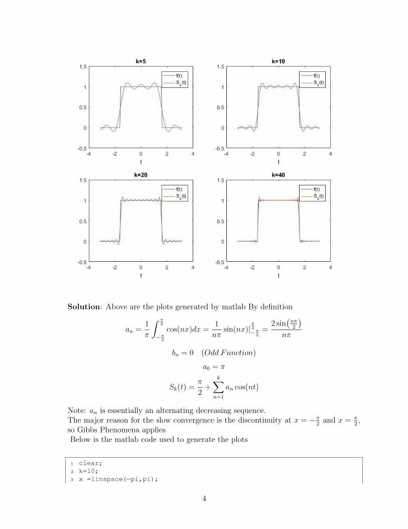
Solution: Above are the plots generated by matlab By definition
an =1
π
∫ π2
−π2
cos(nx)dx =1
nπsin(nx)|
π2
−π2
=2 sin
(nπ2
)nπ
bn = 0 (Odd Function)
a0 = π
Sk(t) =π
2+
k∑n=1
an cos(nt)
Note: an is essentially an alternating decreasing sequence.The major reason for the slow convergence is the discontinuity at x = −π
2and x = π
2,
so Gibbs Phenomena appliesBelow is the matlab code used to generate the plots
1 clear;2 k=10;3 x =linspace(−pi,pi);
4

4 f =ones(100,1);5 f(1:25)=0;6 f(76:end)=0;7 idx=1:k;8 A=zeros(k,100);9 a=2*sin(pi*idx/2)./(pi*idx);
10 for i=1:k11 for j=1:10012 A(i,j)=cos(x(j)*i);13 end14 end15 S k=1/2+a*A;16 plot(x,f,x,S k);
Exercise 3.9 Consider Example 3.9: f(t) = t, 0 ≤ t ≤ π. Is it permissible to differentiatethe Fourier sine series for this function term-by-term? If so, say what the differentiatedseries converges to at each point. Is it permissible to differentiate the Fourier cosineseries for the function f(t) term-by-term? If so, say what the differentiated seriesconverges to at each point.Solution:
Fourier sin:
t ≈∞∑n=1
2(−1)(n+1) sin(nt)
n
Fourier cos:
t ≈ π
2− π
4
∞∑j=1
cos[(2j − 1)t]
(2j − 1)2
Differentiate term-by-term we haveFourier sin:
1 ≈∞∑n=1
2(−1)(n+1) cos(nt)
Which does not converge, since 2(−1)(n+1) cos(nt) does not go to 0Fourier cos:
1 ≈ π
4
∞∑j=1
sin[(2j − 1)t]
(2j − 1)=π
4
∞∑n=1
sin(nt)
n≈ 2− t
π
Exercise 3.10 Derive Lemma 3.24 from expression (3.13) and Lemma 3.23.Solution:
5

θk(t) =1
π
∫ 2π
0
Fk(t− x)f(x)dx (Expression 3.13)
=1
π
∫ 2π
0
Fk(t− x) + Fk(t+ x)
2f(x)dx
=2
π
∫ π
0
Fk(t− x) + Fk(t+ x)
2f(x)dx
=2
kπ
∫ π
0
Fk(t− x) + Fk(t+ x)
2[sin(kx2
)sin x
2
]2dx (Lemma 3.23)
=2
kπ
∫ π2
0
(Fk(t− 2x) + Fk(t+ 2x))[sin(kx)
sin(x)]2dx (Change of variable)
Exercise 3.11 Expand
f(x) = 0 for − π < x ≤ −π
2
1 for − π2< x ≤ π
2
0 for π2< x ≤ π
in a Fourier series on the interval −π ≤ x ≤ π. Plot both f and the arithmetic sum θkfor k = 5, 10, 20, 40. Observe how the arithmetic sums approximate f . Compare withExercise 3.8.Solution:
As you can see in the figure below, the new approximate has a slower convergencerate with respect to mean-square norm (due to the fact we are taking mean values),but better point wise convergence result(no more Gibbs Phenomenon). Below is thematlab code used to generate the plots
1 k=20;2 theta k=0;3 x =linspace(−pi,pi);4 f =ones(100,1);5 f(1:25)=0;6 f(76:end)=0;7 for n=1:k8 idx=1:n;9 A=zeros(n,100);
10 a=2*sin(pi*idx/2)./(pi*idx);11 for i=1:n12 for j=1:10013 A(i,j)=cos(x(j)*i);14 end15 end16 theta k=theta k+1/2+a*A;17 end18 theta k=theta k/k;19 subplot(2,2,3);20 plot(x,f,x,theta k);21 title('k=20');
6

7

22 xlabel('t');23 legend('f(t)','S k(t)')
Exercise 3.12 let f(x) = x, x ∈ [−π, π].(a) Show that f(x) has the Fourier series
∞∑n=1
2
n(−1)n−1 sin(nx).
(b) Let α > 0 Show that f(x) = exp(αx), x ∈ [−π, π] has the Fourier series
(eαπ − e−απ
π)(
1
2α+∞∑k=1
(−1)kα cos(kx)− k sin(kx)
α2 + k2
(c) Let α be any real number other than an integer. Let f(x) = cos(αx), x ∈ [−π, π].Show that f has a Fourier series
sin(απ)
απ+
1
π
∞∑n=1
[sin(α + n)π
α + n+
sin(α− n)π
α− n] cos(nx).
(d) Find the Fourier series of f(x) = −α sin(αx), x ∈ [−π, π]. Do you notice anyrelationship to that in (c)?(e) Find the Fourier series of f(x) = |x|, x ∈ [−π, π].(f) Find the Fourier series of
f(x) = sign(x) = −1, x < 00, x = 01, x > 0
Do you notice any relationship to that in (e)?Solution:
(a) f(x) is odd function, so an = 0
bn =2
π
∫ π
0
x sin(nx)dx
bn =2
π
∫ π
0
x sin(nx)dx
= − 2
πnx cos(nx)
∣∣∣π0
+2
πn
∫ π
0
cos(nx)dx (Integration by Part)
= − 2
ncos(nπ)
=2
n(−1)n−1
8

f(x) = a02
+∑∞
n=1(an cos(nx) + bn sin(nx))
(b)By Euler’s formula we have sin(nx) = einx−e−inx2i
and cos(nx) = einx+e−inx
2
a0 =1
π
∫ π
−πeαxdx =
eαπ − e−απ
απ
an =1
π
∫ π
−πeαx cos(nx)dx
=1
2π[
∫ π
−πe(α+in)xdx+
∫ π
−πe(α−in)xdx]
= (−1)nα
α2 + n2
bn =1
π
∫ π
−πeαx sin(nx)dx
=1
2πi[
∫ π
−πe(α+in)xdx−
∫ π
−πe(α−in)xdx]
= (−1)n−n
α2 + n2
f(x) = a02
+∑∞
n=1(an cos(nx) + bn sin(nx))(c) we can take part (b)’s result, and plug in αi instead of α, and take the real part.The remaining is purely algebraic manipulation.(d) Notice that f(x) = −α sin(αx) = d
dx(cos(αx)), and it’s piecewise smooth so the
Fourier series is:
− 1
π
∞∑n=1
[n sin(α + n)π
α + n+n sin(α− n)π
α− n] sin(nx)
(e) Even function, so bn = 0
a0 =2
π
∫ π
0
xdx = π
an =2
π
∫ π
0
x cos(nx)dx
=2
πnx sin(nx)
∣∣∣π0− 2
πn
∫ π
0
sin(nx)dx (Integration by Part)
=2
πn2[(−1)n − 1]
f(x) =π
2+
2
π
∞∑n=1
(−1)n cos(nx)− cos(nx)
n2
(f) Notice that f(x) is the derivative of the function in (e), and it’s piecewise smooth,so the Fourier series is:
f(x) =2
π
∞∑n=1
(−1)n−1 sin(nx) + sin(nx)
n
9

Exercise 3.13 Sum the series∑∞
n=0 2−n cos(nt), and∑∞
n=0 2−n sin(nt).Hint: Take the real and imaginary parts of the
∑∞n=0 2−neint You should be able to
sum this last series directly. Solution:
∞∑n=0
2−neint =1
1− eit
2
(Sum of GeometricSeries)
=2
2− cos(t)− i sin(t)
=4− 2 cos(t) + 2i sin(t)
5− 4 cos(t)
So the cos sum is:4− 2 cos(t)
5− 4 cos(t)
The sin sum is:2 sin(t)
5− 4 cos(t)
Exercise 3.14 Find the L2[−π, π] projection of the function f1(x) = x2 onto the (2n+ 1)-dimensional subspace spanned by the ON set
1√2π,cos(kx)√
π,sin(kx)√
π: k = 1, ..., n
for n=1. Repeat for n=2,3. Plot these projections along with f1. Repeat the wholeexercise for f2(x) = x3. Do you see any marked differences between the graphs in thetwo cases?Solution:
For f1(x), it is an even function, so bn = 0,
a0 =2
π
∫ π
0
x2dx =2π2
3
Similar to calculation with Excercise 3.12(a), but this time with two-steps of integrationby part, we have:
an =2
π
∫ π
0
x2 cos(nx)dx
=4
n2(−1)n
For f2(x), it is an odd function, so an = 0, Similar to calculation above, but this timewith three-steps of integration by part, we have:
bn =2
π
∫ π
0
x3 sin(nx)dx
=12
n3(−1)n − 2π2(−1)n
n
Below is the matlab code used to generate the plots
10

11

1 x=linspace(−pi,pi);2 f1=x.ˆ2;3 f2=x.ˆ3;4 k=3;5 idx=1:k;6 A1=zeros(k,100);7 A2=zeros(k,100);8 a1=4*(−1).ˆidx./(idx.ˆ2);9 a2=12*((−1).ˆidx)./(idx.ˆ3)−2*piˆ2*((−1).ˆidx)./idx;
10 for i=1:k11 for j=1:10012 A1(i,j)=cos(x(j)*i);13 A2(i,j)=sin(x(j)*i);14 end15 end16 S1 k=piˆ2/3+a1*A1;17 S2 k=a2*A2;18
19 subplot(2,3,3);20 plot(x,f1,x,S1 k);21 title('k=3');22 xlabel('t');23 legend('f1(t)','S1 k(t)')24 subplot(2,3,6);25 plot(x,f2,x,S2 k);26 title('k=3');27 xlabel('t');28 legend('f2(t)','S2 k(t)')
Notice that we can interpret f1(x) = 13( ddx
(f2(x))) Because f1(x) is continuous, howeverfx(x) has a point of discontinuity at the edge, we observe Gibbs Phenomenon in f2(x)but not in f1(x)
Exercise 3.15 By substituting special values of x in convergent Fourier series, we can of-ten deduce interesting series expansions for various numbers, or just find the sum ofimportant series.(a) Use the Fourier series for f(x) = x2 to show that
∞∑n=1
(−1)n−1
n2=π2
12
(b) Prove that Fourier series for f(x) = x converges in (−π, π) and hence that∞∑l=0
(−1)l
2l + 1=π
4
(c) Show that the Fourier series of f(x) = exp(αx), x ∈ [−π, π] converges in [−π, pi)to exp(αx) and at x = π to exp(αpi)+exp(−αpi)
2. Hence show that
απ
tanh(απ) = 1 +∑∞
k=12α2
k2+α2
12

(d) Show that
π
4=
1
2+∞∑n=1
(−1)n−1
4n2 − 1.
(e) Plot both f(x) = x2 and the partial sums
Sk(x) =a02
+∞∑n=0
(an cos(nx) + bn sin(nx))
for k=1,2,5,7. Observe how the partial sums approximate f .Solution:
(a) The Fourier series is already derived in Exercise 3.14, since f(x) has smooth deriva-tive, it’s Fourier Series converges point-wise in (−π, π), take x = 0, we obtained thedesired equality.(b) The Fourier series is already derived in Exercise 3.12(a), since f(x) has smoothderivative in (−π, π), the series converge within the same range. Then take x = π
2we
obtained the desired equality.(c) The Fourier series is already derived in Exercise 3.12(b), since f(x) has smoothderivative in (−π, π), the series converge within the same range. And since its deriva-tive is right-continuous at −π and left-continuous at π, then at point π it converges tothe average of the two limit, which is exp(αpi)+exp(−αpi)
2.
Then take x = π we obtained the desired equality.(d) Follow the Fourier series obtained in Exercise 3.12(c), take α = 1
2and x = 0, we
obtained the desired equality (e) Identical Result to Exercise 3.14
Exercise 3.16 Let f1(x) = x and f2(x) = π2 − 3x2,−π ≤ t ≤ π. Find the Fourier series off1 and f2 and use them alone to sum the following series:
1.∑∞
n=1(−1)n2n+1
2.∑∞
n=11n2
3.∑∞
n=1(−1)nn2
4.∑∞
n=11n4
Solution: Fourier series f1(x) is already obtained as in Exercise 3.12(a) For f2(x) it’sa modified version from Exercise 3.14, we can obtained it’s Fourier series easily:
f2(x) =∞∑n=1
12(−1)n−1
n2
1. Directly obtained from Excercise 3.15(b), it’s equal to∑∞
n=1(−1)n2n+1
= pi4− 1
2. Take x = π for f2(x), we have∑∞
n=11n2 = π
6
3. Multiply by -1 to Exercise 3.15(a),∑∞
n=1(−1)nn2 = −π2
12
4. Apply Parseval’s identity to f2(x), we have∑∞
n=11n4 = π4
90
13

Exercise 3.17 By Applying Parseval’s identity to suitable Fourier Series:(a) show that
∞∑n=1
1
n4=π4
90.
(b) Evaluate∞∑n=1
1
α2 + n2.
(c) Show that∞∑l=0
1
(2l + 1)4=π4
96.
Solution:
(a) Same as Exercise 3.16.4(b) From Exercise 3.15 (c):
∞∑n=1
1
α2 + n2=
π
2α tanh(απ)− 1
2α2
(c) Apply Parseval’s identity to f(x) = |x|, note (−1)n−1 = 0forneven and (−1)n−1 =−2fornodd
π2
2+∞∑l=0
16
(2l + 1)4=
2π2
3
Thus we obtained the quality desired
Exercise 3.18 Is∞∑n=1
cos(nx)
n1/2
The Fourier series of some square integrable function f on [−π, π]?The same question for the series
∞∑n=1
cos(nx)
log(n+ 2)
Solution:
Neither of them are.Prove By contradition, assume they are, then they will satisfy Parseval’s identityHowever, neither of the series sum converge (in fact they diverge to infinity):
∑∞n=1
1n
note: Famous divergent series, and can apply integral test to prove it’s a divergentseries)∑∞
n=11
[log(n+2)]2, apply comparison test with the series above so neither of them can be
the Fourier series of some square integrable function
14

Solutions to Chapter 4
Exercise 4.1 Verify the rules for Fourier transforms listed above.
Solution:
F [af + bg] =1√2π
∫ ∞−∞
(af(t) + bg(t))e−iλtdt
= a1√2π
∫ ∞−∞
f(t)e−iλtdt+ b1√2π
∫ ∞−∞
g(t)e−iλtdt
= aF [f ] + bF [g].
F∗[af + bg] =1√2π
∫ ∞−∞
(af(λ) + bg(λ))eiλtdλ
= a1√2π
∫ ∞−∞
f(λ)eiλtdλ+ b1√2π
∫ ∞−∞
g(λ)eiλtdλ
= aF∗[f ] + bF∗[g].
F [tnf(t)](λ) =1√2π
∫ ∞−∞
tnf(t)e−iλtdt
=1√2π
1
(−i)ndn
dλn
∫ ∞−∞
f(t)e−iλtdt
= indn
dλnF [f ](λ).
F∗[λnf(λ)](t) =1√2π
∫ ∞−∞
λnf(λ)eiλtdλ
=1√2π
1
indn
dtn
∫ ∞−∞
f(λ)eiλtdλ
= (−i)n dn
dλnF [f ](λ).
Since
F [f ′](λ) =1√2π
∫ ∞−∞
f ′(t)e−iλtdt
=1√2πf(t)e−iλt
∣∣∣∞t=−∞
− 1√2π
∫ ∞−∞
(−iλ)f(t)e−iλtdt
= iλ1√2π
∫ ∞−∞
f(t)e−iλtdt = iλF [f ](λ),
thusF [f (n)](λ) = (iλ)nF [f ](λ).
1
Since
F∗[f ′](t) =1√2π
∫ ∞−∞
f ′(λ)eiλtdλ
=1√2πf(λ)eiλt
∣∣∣∞λ=−∞
− 1√2π
∫ ∞−∞
(it)f(λ)eiλtdλ
= −it 1√2π
∫ ∞−∞
f(λ)eiλtdλ = −itF [f ](λ),
thusF∗[f (n)](t) = (−it)nF∗[f ](t).
Let bt− a = r, then t = r/b+ a/b, dt = dr/b and
F [f(bt− a)](λ) =1√2π
∫ ∞−∞
f(bt− a)e−iλtdt
=1√2π
∫ ∞−∞
1
bf(r)e−i(r/b+a/b)λdr
=1
be−iλa/b
1√2π
∫ ∞−∞
f(r)e−iλr/bdr =1
be−iλa/bF [f ](
λ
b).
Exercise 4.2 Let f, g, h : R→ R. Let a, b ∈ R, show that:
(i) Convolution is linear:
(af + bg) ∗ h = a(f ∗ h) + b(g ∗ h).
(ii) Convolution is commutative:
f ∗ g = g ∗ f
(iii) Convolution is associative:
(f ∗ g) ∗ h = f ∗ (g ∗ h)
Solution: (i)
(af + bg) ∗ h =
∫ ∞−∞
(af(x) + bg(x))h(t− x)dx
= a
∫ ∞−∞
f(x)h(t− x)dx+ b
∫ ∞−∞
g(x)h(t− x)dx
= a(f ∗ h) + b(g ∗ h).
(ii) Let y = t− x, then x = t− y, dx = −dy and
f ∗ g =
∫ ∞−∞
f(x)g(t− x)dx
= −∫ −∞∞
f(t− y)g(y)dy
=
∫ ∞−∞
f(t− y)g(y)dy = g ∗ f.
2

(iii)
(f ∗ g) ∗ h =
∫ ∞−∞
(∫ ∞−∞
f(x)g(y − x)dx
)h(t− y)dy
Let y = x+ z, then∫ ∞−∞
(∫ ∞−∞
f(x)g(y − x)dx
)h(t− y)dy =
∫ ∞−∞
f(x)
(∫ ∞−∞
g(z)h(t− x− z)dz
)dx
=
∫ ∞−∞
f(x)(g ∗ h)(t− x)dx
= f ∗ (g ∗ h).
Exercise 4.3 Let
Π(t) =
1 for − 1
2< t < 1
2
0 otherwise,
the box function on the real line. We will often have the occasion to express the Fouriertransform of f(at+b) in terms of the Fourier transform f(λ) of f(t), where a, b are realparameters. This exercise will give you practice in correct application of the transform.
1. Sketch the graphs of Π(t), Π(t− 3) and π(2t− 3) = Π(2(t− 3/2)).
2. Sketch the graphs of Π(t), Π(2t) and Π(2(t − 3)). Note: In the first part a right3-translate is followed by a 2-dilate; but in the second part a 2-dilate is followed by aright 3-translate. The results are not the same.
3. Find the Fourier transforms of g1(t) = Π(2t− 3) and g2(t) = Π(2(t− 3)) from parts1 and 2.
4. Set g(t) = Π(2t) and check your answers to part 3 by applying the translation ruleto
g1(t) = g(t− 3
2), g2(t) = g(t− 3), noting g2(t) = g1(t−
3
2).
Solution: 1. See Figure 1.
2. See Figure 2.
3.
F [g1](λ) =1√2π
∫ ∞−∞
g1(t)e−iλtdt
=1√2π
∫ 7/4
5/4
e−iλtdt
=2e−3iλ/2 sin(λ/4)√
2πλ
3

Figure 1:
Figure 2:
F [g2](λ) =1√2π
∫ ∞−∞
g1(t)e−iλtdt
=1√2π
∫ 13/4
11/4
e−iλtdt
=2e−3iλ sin(λ/4)√
2πλ
4. Since
F [g](λ) =2 sin(λ/4)√
2πλ,
thenF [g1](λ) = e−3iλ/2F [g](λ), F [g2](λ) = e−3iλF [g](λ).
Exercise 4.4 Assuming that the improper integral∫∞0
(sinx/x)dx = I exists, establish its
4

value (2.1) by first using the Riemann-Lebesgue lemma for Fourier series to show that
I = limk→∞
∫ (k+1/2)π
0
sinx
xdx = lim
k→∞
∫ π
0
Dk(u)du
where Dk(u) is the Dirichlet kernel function. Then use Lemma 3.11.
Solution: Let x = (k + 1/2)u, then dx = (k + 1/2)du and
limk→∞
∫ (k+1/2)π
0
sinx
xdx = lim
k→∞
∫ π
0
sin(k + 1/2)u
udu
= limk→∞
∫ δ
0
sin(k + 1/2)u
udu+ lim
k→∞
∫ π
δ
sin(k + 1/2)u
udu.
The second part of the integral is zero and it can be replaced as
limk→∞
∫ π
δ
sin(k + 1/2)u
udu = 0 = lim
k→∞
∫ π
δ
sin(k + 1/2)u
2 sin(u/2)du.
If δ is sufficient small and u ∈ [0, δ], u↔ 2 sin(u/2), thus the first part of the integralcan be replaced as
limk→∞
∫ δ
0
sin(k + 1/2)u
udu = lim
k→∞
∫ δ
0
sin(k + 1/2)u
2 sin(u/2)du.
Consequently, we have
limk→∞
∫ π
0
sin(k + 1/2)u
udu = lim
k→∞
∫ π
0
sin(k + 1/2)u
2 sin(u/2)du,
where ∫ π
0
sin(k + 1/2)u
2 sin(u/2)du =
∫ π
0
(1
2+
k∑n=1
cosnu
)du =
π
2.
Exercise 4.5 Define the right-hand derivative f ′R(t) and the left-hand derivative f ′L(t) of fby
f ′R(t) = limu→t+
f(u)− f(t+ 0)
u− t, f ′L(t) = lim
u→t−
f(u)− f(t− 0)
u− t,
respectively, as in Exercise 3.4. Show that in the proof of Theorem 4.17 we can dropthe requirements 3 and 4, and the right-hand side of (4.12) will converge to (t+0)+f(t−0)
2
at any point t such that both f ′R(t) and f ′L(t) exist.
Solution: In the proof of Theorem 4.17∫ c
0
(f(t+ x) + f(t− x))sinLx
πxdx =
∫ c
0
f(t+ x)sinLx
πxdx+
∫ c
0
f(t− x)sinLx
πxdx,
when L→∞, in the right hand side, the first part will converge to f(t+ 0)/2 if f ′R(t)exist and the second part will converge to f(t − 0)/2 if f ′L(t) exist. Hence, the total
result converge to (t+0)+f(t−0)2
.
5
Exercise 4.6 Let a > 0. Use the Fourier transforms of sinc (x) and sinc 2(x), together withthe basic tools of Fourier transform theory, such as Parseval’s equation, substitution,... to show the following. (Use only rules from Fourier transform theory. You shouldn’tdo any detailed computation such as integration by parts.)
•∫∞−∞
(sin axx
)3dx = 3a2π
4
•∫∞−∞
(sin axx
)4dx = 2a3π
3
Solution: ∫ ∞−∞
(sin ax
x
)3
dx = a3∫ ∞−∞
(sin ax
ax
)2(sin ax
ax
)dx
= a3∫ ∞−∞F
[(sin ax
ax
)2]
(λ)F[
sin ax
ax
](λ)dλ
= a3∫ ∞−∞
√π√
2a2tri
(λ
2a
) √π√
2a2rect
(λ
2a
)dλ
=πa
2
∫ a
−atri
(λ
2a
)dλ
= πa
∫ a
0
(1− λ
2a
)dλ =
3a2π
4.
∫ ∞−∞
(sin ax
x
)4
dx = a4∫ ∞−∞
(sin ax
ax
)2(sin ax
ax
)2
dx
= a4∫ ∞−∞F
[(sin ax
ax
)2]
(λ)F
[(sin ax
ax
)2]
(λ)dλ
= a4∫ ∞−∞
√π√
2a2tri
(λ
2a
) √π√
2a2tri
(λ
2a
)dλ
=πa2
2
∫ 2a
−2atri2(λ
2a
)dλ
= πa2∫ 2a
0
(1− λ
2a
)2
dλ =2a3π
3.
Exercise 4.7 Show that the n-translates of sinc are orthonormal:∫ ∞−∞
sinc (x− n) · sinc (x−m)dx =
1 for n = m0 otherwise,
n,m = 0,±1, . . .
6

Solution:∫ ∞−∞
sinc (x− n) · sinc (x−m)dx =
∫ ∞−∞F [sinc (x− n)](λ) · F [sinc (x−m)](λ)dλ
=1
2π
∫ ∞−∞
rect2(λ
2π
)e−i(n−m)λdλ
=1
2π
∫ π
−πe−i(n−m)λdλ.
Hence,1
2π
∫ π
−πe−i(n−m)λdλ =
1 for n = m0 otherwise,
n,m = 0,±1, . . .
Exercise 4.8 Let
f(t) =
1 −2 ≤ t ≤ −11 1 ≤ t ≤ 20 otherwise.
• Compute the Fourier transform f(λ) and sketch the graphs of f and f .
• Compute and sketch the graph of the function with Fourier transform f(−λ).
• Compute and sketch the graph of the function with Fourier transform f ′(λ).
• Compute and sketch the graph of the function with Fourier transform f ∗ f(λ).
• Compute and sketch the graph of the function with Fourier transform f(λ/2).
Solution:
• f(t) = rect(t+ 3/2) + rect(t− 3/2), thus
f(λ) = (e−3iλ/2 + e3iλ/2)sinc (λ
2π) = 2 cos(3λ/2)sinc (
λ
2π).
See Figure 3.
• f(−λ) = f(λ) = f(λ).
•
f ′(λ) =√
2πF [−itf(t)](λ) =2(−λ cos(λ) + 2λ cos(2λ) + sin(λ)− sin(2λ))
λ2
See Figure 4.
• f ∗ f(λ) = (2π)3/2F [f 2(t)](λ) = (2π)3/2F [f(t)](λ) = 2πf(λ). See Figure 5.
• f(λ/2) = 2√
2πF [f(2t)](λ). See Figure 6.
7

-3 -2 -1 0 1 2 3
t
0
0.2
0.4
0.6
0.8
1
-10 -5 0 5 10-2
-1.5
-1
-0.5
0
0.5
1
1.5
2
Figure 3: f(t) and f(λ)
-10 -8 -6 -4 -2 0 2 4 6 8 10-3
-2
-1
0
1
2
3
Figure 4: f ′(λ)
Exercise 4.9 Deduce what you can about the Fourier transform f(λ) if you know that f(t)satisfies the dilation equation
f(t) = f(2t) + f(2t− 1)
8

-10 -8 -6 -4 -2 0 2 4 6 8 10-15
-10
-5
0
5
10
15
Figure 5: f ∗ f(λ)
-10 -8 -6 -4 -2 0 2 4 6 8 10-2
-1.5
-1
-0.5
0
0.5
1
1.5
2
Figure 6: f(λ/2)
9

Solution:
f(λ) =1
2f
(λ
2
)+e−iλ/2
2f
(λ
2
)=
1 + e−iλ/2
2f
(λ
2
)Exercise 4.10 Just as Fourier series have a complex version and a real version, so does the
Fourier transform. Under the same assumptions as Theorem 4.17 set
C(α) =1
2
[f(α) + f(−α)
], S(α) =
1
2i
[−f(α) + f(−α)
], α ≥ 0
and derive the expansion
f(t) =1
π
∫ ∞0
(C(α) cosαt+ S(α) sinαt
)dα,
C(α) =
∫ ∞−∞
f(s) cos(αs)ds, S(α) =
∫ ∞−∞
f(s) sin(αs)ds.
Show that the transform can be written in a more compact form as
f(t) =1
π
∫ ∞0
dα
∫ ∞−∞
f(s) cosα(s− t)ds
Solution:1
π
∫ ∞0
(C(α) cosαt+ S(α) sinαt
)dα
=1
2π
∫ ∞0
(f(α)(cosαt+ i sinαt) + f(−α)(cos(−αt) + i sin(−αt))
)dα
=1
2π
∫ ∞−∞
f(α)(cosαt+ i sinαt)dα
=1
2π
∫ ∞−∞
f(α)eiαtdα = f(t).
C(α) =1
2
[∫ ∞−∞
f(s)e−iαsds+
(∫ ∞−∞
f ∗(s)e−iαsds
)∗]=
1
2
[∫ ∞−∞
f(s)e−iαsds+
∫ ∞−∞
f(s)eiαs]
=1
2
∫ ∞−∞
f(s)(e−iαs + eiαs
)ds
=
∫ ∞−∞
f(s) cos(αs)ds
S(α) =1
2i
[−∫ ∞−∞
f(s)e−iαsds+
(∫ ∞−∞
f ∗(s)e−iαsds
)∗]=
1
2i
[−∫ ∞−∞
f(s)e−iαsds+
∫ ∞−∞
f(s)eiαs]
=1
2i
∫ ∞−∞
f(s)(−e−iαs + eiαs
)ds
=
∫ ∞−∞
f(s) sin(αs)ds
10

Substitute the expansion of C(α) and S(α) into the expansion of f(t), then we have
f(t) =1
π
∫ ∞0
(∫ ∞−∞
f(s) cos(αs) cos(αt)ds+
∫ ∞−∞
f(s) sin(αs) sin(αt)ds
)dα
=1
π
∫ ∞0
(∫ ∞−∞
f(s)(cos(αs) cos(αt) + sin(αs) sin(αt))ds
)dα
=1
π
∫ ∞0
dα
∫ ∞−∞
f(s) cosα(s− t)ds
Exercise 4.11 There are also Fourier integral analogs of the Fourier cosine series and theFourier sine series. Let f(t) be defined for all t ≥ 0 and extend it to an even functionon the real line, defined by
F (t) =
f(t), if t ≥ 0f(−t), if t < 0
By applying the results of Exercise 4.10 show that, formally,
f(t) =2
π
∫ ∞0
cosαt dα
∫ ∞0
f(s) cosαs ds, t ≥ 0
Find conditions on f(t) such that this pointwise expansion is rigorously correct.
Solution: According to the result of Exercise 4.10,
F (t) =1
π
∫ ∞0
dα
∫ ∞−∞
F (s) cosα(s− t)ds
=1
π
∫ ∞0
cosαt dα
∫ ∞−∞
F (s) cosαs ds+1
π
∫ ∞0
sinαt dα
∫ ∞−∞
F (s) sinαs ds.
Since F (s), cosαs are even functions and sinαs is odd function, we have∫ ∞−∞
F (s) cosαs ds = 2
∫ ∞0
F (s) cosαs ds = 2
∫ ∞0
f(s) cosαs ds,
∫ ∞−∞
F (s) sinαs ds = 0.
Thus, for t ≥ 0
f(t) = F (t) =2
π
∫ ∞0
cosαt dα
∫ ∞0
f(s) cosαs ds.
If f(t) satisfies the assumptions in Theorem 4.17, this pointwise expansion is rigorouslycorrect.
11
Exercise 4.12 Let f(t) be defined for all t > 0 and extend it to an odd function on the realline, defined by
G(t) =
f(t), if t > 0−f(−t), if t < 0
By applying the results of Exercise 4.10 show that, formally
f(t) =2
π
∫ ∞0
sinαt dα
∫ ∞0
f(s) sinαs ds, t > 0
Find conditions on f(t) such that this pointwise expansion is rigorously correct.
Solution: According to the result of Exercise 4.10,
G(t) =1
π
∫ ∞0
dα
∫ ∞−∞
F (s) cosα(s− t)ds
=1
π
∫ ∞0
cosαt dα
∫ ∞−∞
G(s) cosαs ds+1
π
∫ ∞0
sinαt dα
∫ ∞−∞
G(s) sinαs ds.
Since cosαs is even function and G(s), sinαs are odd functions, we have∫ ∞−∞
G(s) cosαs ds = 0,
∫ ∞−∞
G(s) sinαs ds = 2
∫ ∞0
G(s) sinαs ds = 2
∫ ∞0
f(s) sinαs ds.
Thus, for t > 0
f(t) = G(t) =2
π
∫ ∞0
sinαt dα
∫ ∞0
f(s) sinαs ds.
If f(t) satisfies the assumptions in Theorem 4.17, this pointwise expansion is rigorouslycorrect.
Exercise 4.13 Find the Fourier Cosine and Sine transforms of the following functions:
f(t) :=
1, t ∈ [0, a]0, t > a
f(t) :=
cos(at), t ∈ [0, a]0, t > a
Solution: For the first function,
f c(α) =
∫ ∞−∞
f(t) cos(αt)dt
=
∫ a
0
cos(αt)dt =1
αsin(aα)
12

f s(α) =
∫ ∞−∞
f(t) sin(αt)dt
=
∫ a
0
sin(αt)dt =1
α(1− cos(aα))
For the second function,
f c(α) =
∫ ∞−∞
f(t) cos(αt)dt
=
∫ a
0
cos(at) cos(αt)dt
=a cos(aα) sin(a2)− α cos(a2) sin(aα)
a2 − α2
f s(α) =
∫ ∞−∞
f(t) sin(αt)dt
=
∫ a
0
cos(at) sin(αt)dt
=α cos(a2) cos(aα) + a sin(a2) sin(aα)− α
a2 − α2
Exercise 4.14 Use the fact that f(t) = sinc (t + a) is frequency bandlimited with B = πto show that
sinc (t+ a) =∞∑
j=−∞
sinc (j + a)sinc (t− j)
for all a, t. Derive the identity
1 =∞∑
j=−∞
sinc 2(t− j).
Solution: Since we have the Fourier transform
f(t+ a)←→ eiaλf(λ),
Substitute f(t), f(λ) and B in the proof of Theorem 4.18 with f(t+ a), eiaλf(λ) andπ, respectively. Then, we have
eiaλf(λ) =∞∑
k=−∞
ckeikλ, ck =
1
2π
∫ π
π
f(λ)ei(a−k)λ,
thus,
f(t+a) = sinc (t+a) =1
2π
∫ ∞−∞
eiaλf(λ)eiλtdλ =1
2π
∞∑−∞
ck
∫ π
−πei(k+t)λdλ =
∞∑k=−∞
cksinc (t+k),
13

where
ck =1
2π
∫ pi
−πf(λ)ei(a−k)λdλ = f(−k + a) = sinc (−k + a).
Hence, setting k = −j,
sinc (t+ a) =∞∑
j=−∞
sinc (j + a)sinc (t− j).
Let a = −t, then sinc (t + a) = sinc (0) = 1, and sinc (j − t) = sinc (t − j) sincesinc (x) is an even function. Thus, we have
1 =∞∑
j=−∞
sinc 2(t− j).
Exercise 4.15 Suppose f(t) satisfies the conditions of Theorem 4.18. Derive the Parsevalformula ∫ ∞
−∞|f(t)|2dt =
1
2π
∫ ∞−∞|f(λ)|2dλ =
π
B
∞∑k=−∞
|f(πk
B)|2
Solution: ∫ ∞−∞|f(t)|2dt =
1
2π
∫ ∞−∞|f(λ)|2dλ
is valid from the property of Fourier transform. We only prove that∫ ∞−∞|f(t)|2dt =
π
B
∞∑−∞
|f(πk
B)|2.
Since
f(t) =∞∑
j=−∞
f(jπ
B)sinc (
Bt
π− j),
then∫ ∞−∞|f(t)|2dt =
∫ ∞−∞
(∞∑
j=−∞
f(jπ
B)sinc (
Bt
π− j)
)(∞∑
i=−∞
f(iπ
B)sinc (
Bt
π− i)
)∗dt
=∞∑
i,j=−∞
f(jπ
B)f ∗(
iπ
B)
∫ ∞−∞
sinc (Bt
π− j)sinc (
Bt
π− i)dt.
Due to the orthogonal property that∫ ∞−∞
sinc (Bt
π− j)sinc (
Bt
π− i)dt =
Bπ, i = j
0, i 6= j,
then we have ∫ ∞−∞|f(t)|2dt =
π
B
∞∑k=−∞
|f(πk
B)|2.
14
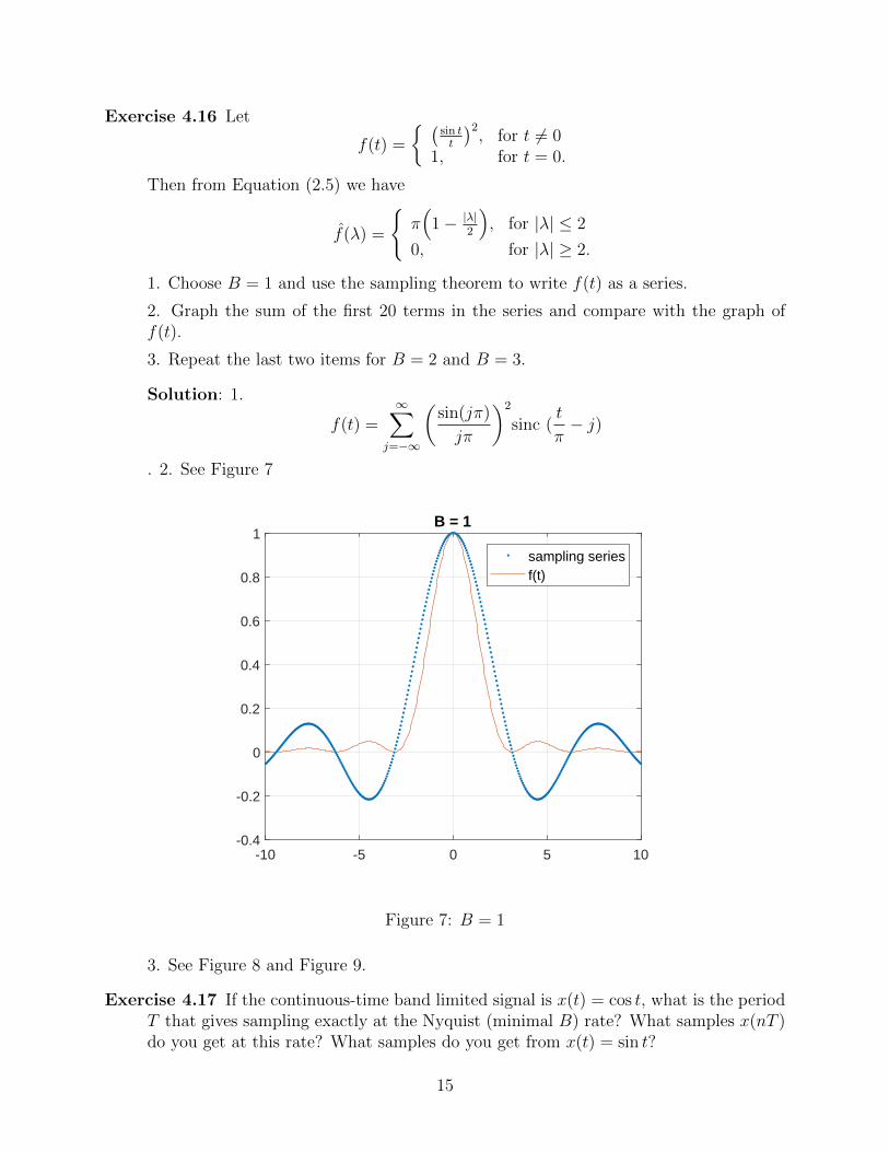
Exercise 4.16 Let
f(t) =
(sin tt
)2, for t 6= 0
1, for t = 0.
Then from Equation (2.5) we have
f(λ) =
π(
1− |λ|2
), for |λ| ≤ 2
0, for |λ| ≥ 2.
1. Choose B = 1 and use the sampling theorem to write f(t) as a series.
2. Graph the sum of the first 20 terms in the series and compare with the graph off(t).
3. Repeat the last two items for B = 2 and B = 3.
Solution: 1.
f(t) =∞∑
j=−∞
(sin(jπ)
jπ
)2
sinc (t
π− j)
. 2. See Figure 7
-10 -5 0 5 10-0.4
-0.2
0
0.2
0.4
0.6
0.8
1B = 1
sampling seriesf(t)
Figure 7: B = 1
3. See Figure 8 and Figure 9.
Exercise 4.17 If the continuous-time band limited signal is x(t) = cos t, what is the periodT that gives sampling exactly at the Nyquist (minimal B) rate? What samples x(nT )do you get at this rate? What samples do you get from x(t) = sin t?
15
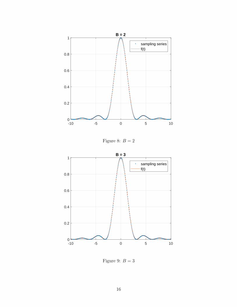
-10 -5 0 5 100
0.2
0.4
0.6
0.8
1B = 2
sampling seriesf(t)
Figure 8: B = 2
-10 -5 0 5 100
0.2
0.4
0.6
0.8
1B = 3
sampling seriesf(t)
Figure 9: B = 3
16

Solution: For x(t) = cos t, x(λ) = π(δ(λ− 1) + δ(λ+ 1)). Thus, Bmin = 1 andT = π/Bmin = π. Consequently, x(nT ) = x(nπ) = cos(nπ).
Similarly, for x(t) = sin t, x(λ) = −iπ(δ(λ− 1)− δ(λ+ 1)). Thus, Bmin = 1 andT = π/Bmin = π. Consequently, x(nT ) = x(nπ) = sin(nπ).
Exercise 4.18 Show that the function
h(λ) =
exp(
11−λ2
), if− 1 < λ < 1
0, if|λ| ≥ 1,
is infinitely differentiable with compact support. In particular compute the derivativesdn
dλnh(±1) for all n.
Solution: limλ→±1dn
dλnh(λ)⇒ ±∞
Exercise 4.19 Construct a function g(λ) which (1) is arbitrarily differentiable, (2) hassupport contained in the interval [−4, 4] and (3) g(λ) = 1 for λ ∈ [1, 1]. Hint: Considerthe convolution 1
2cR[−2,2] ∗ h2(λ) where R[−2,2] is the rectangular box function on the
interval [−2, 2], h2(λ) = h(λ/2), h is defined in Exercise 4.18 and c =∫∞−∞ h(λ)dλ.
Solution: Problematic because of Exercise 4.18, and c→∞ is indefinite.
Exercise 4.20 Let f(t) = at2+a2
for a > 0.
• Show that f(t) = πe−a|λ|. Hint: It is easier to work backwards.
• Use the Poisson summation formula to derive the identity
∞∑n=−∞
1
n2 + a2=π
a
1 + e−2πa
1− e−2πa
What happens as a→ 0+? Can you obtain the value of∑∞
n=11n2 from this?
Solution:
1
2π
∫ ∞−∞
f(λ)eiλtdλ =
∫ ∞0
e−aλ+iλtdλ =e−aλ+iλt
−a+ it
∣∣∣∣∞λ=0
=a+ it
t2 + a2,
thus,
Re
(a+ it
t2 + a2
)=
a
t2 + a2= f(t).
By using the Poisson summation,
∞∑n=−∞
f(n) =∞∑
n=−∞
f(2πn),
17
we have
∞∑n=−∞
1
n2 + a2=
∞∑n=−∞
π
ae−a|2πn|
=π
a+
2π
a
∞∑n=1
e−2naπ
=π
a+
2π
a
e−2πa
1− e−2πa=π
a
1 + e−2πa
1− e−2πa.
Since∞∑
n=−∞
1
n2 + a2=
1
a2+ 2
∞∑n=1
1
n2 + a2,
then
∞∑n=1
1
n2 + a2=
1
2
(π
a
1 + e−2πa
1− e−2πa− 1
a2
)=
1 + πa+ e2πa(−1 + πa)
2a2(−1 + e2πa).
Hence,
lima→0+
1 + πa+ e2πa(−1 + πa)
2a2(−1 + e2πa)= lim
a→0+
23π3a3 +O(a4)
4πa3 +O(a4)=π2
6=∞∑n=1
1
n2
Exercise 4.21 Verify Equations (4.22).
Solution: As
‖f‖2 =
∫ ∞−∞|f(t)|2dt =
∫ ∞−∞
f(t) · f(t)dt,
then
‖g‖2 =
∫ ∞−∞
g(t) · g(t)dt =
∫ ∞−∞
f(t+ t0) · f(t+ t0)e−iλ0t+iλ0td(t+ t0)
=
∫ ∞−∞
f(s)f(s)ds = ‖f‖2.
According to Plancherel identity
2π‖f‖2 = ‖f‖2, 2π‖g‖2 = ‖g‖2,
then we have‖f‖2 = ‖g‖2.
Consequently,
D0g =
∫ ∞−∞
t2|g(t)|2
‖g‖2dt =
∫ ∞−∞
t2|f(t+ t0)|2
‖f‖2dt
s:=t+t0=
∫ ∞−∞
(s− t0)2|f(s)|2
‖f‖2ds = Dt0f.
18
Sinceg(t) = f(λ+ λ0)e
it0λ,
then
D0g =
∫ ∞−∞
λ2|g(λ)|2
‖g‖2dλ =
∫ ∞−∞
λ2|f(λ+ λ0)|2
‖f‖2dλ
s:=λ+λ0=
∫ ∞−∞
(s−λ0)2|f(s)|2
‖f‖2ds = Dλ0 f .
Exercise 4.22 Let
f(t) =
0, if t < 0√
2e−t, if t ≥ 0
Compute (Dt0f)(Dλ0 f) for any t), λ0 ∈ R and compare with Theorem 4.21.
Solution: Since ‖f‖2 =∫∞0
2e−2tdt = 1 = 12π‖f‖2, and f(λ) =
√2 1−iλλ2+1
then
Dt0f =
∫ ∞0
(t− t0)22e−2tdt = t20 − t0 +1
2,
Dλ0 f =
∫ ∞−∞
(λ− λ0)2
π(λ2 + 1)dλ = undefined(→∞).
Hence, (Dt0f)(Dλ0 f)→∞ ≥ 1/4.
Exercise 4.23 Show that the eigenvalues of a covariance matrix are nonnegative.
Solution: Since C = E((t− u)(t− u)T
), for arbitrary vector v 6= 0,
vTCv = E(vT (t− u)(t− u)Tv
)= E(s2) ≥ 0,
where s = vT (t−u) = (t−u)Tv is a scalar random viable. Therefore, C is semidefinitepositive and its eigenvalues are nonnegative.
Exercise 4.24 Show that C is in fact the covariance matrix of the distribution (4.24). Thistakes some work and involves making an orthogonal change of coordinates where thenew coordinate vectors are the orthonormal eigenvectors of C.
Solution: Since C is semidefinite positive, we have the eigen-decomposition C =V ΛV T , where V is an orthonormal matrix consisted the eigenvectors of C, and Λ is adiagonal matrix that Λ = diag(σ2
1, σ22, . . . , σ
2n) with σ2
i ≥ 0.
Let s be the new coordinates of random variables t under the coordinate transformV , then we have t = V s and µ = E(t) = E(V s) = V · E(s) = V ν, or alternativelys = V T t and ν = V Tµ. Due to the eigen-decomposition, under this new coordinatesystem we have
E((si − νi)(sj − νj)) =
σ2i , i = j
0, i 6= j,
19

which means that s1, s2, . . . , sn are independent. Thus, the multivariate normaldistribution under the new coordinate system is
ρ(s) =1√
(2π)n∏n
i=1 σ2i
exp
[n∑i=1
(−(si − νi)2
2σ2i
)]
=1√
(2π)n det(C)exp
[1
2(s− ν)Tdiag(σ−21 , σ−22 , . . . , σ−2n )(s− ν)
]=
1√(2π)n det(C)
exp
[1
2(t− µ)TV Λ−1V T (t− µ)
]=
1√(2π)n det(C)
exp
[1
2(t− µ)TC−1(t− µ)
]= ρ(t).
Exercise 4.25 If the random variables are independently distributed, show that
C(ti, tj) = σ2i δij
Solution: If the random variables are independently distributed, the covariance of anypair (ti, tj) is zero if i 6= j. This is because that
E((ti − µi)(tj − µj)) = E(titj)− E(ti)E(tj).
If ti, tj are independent, E(titj) = E(ti)E(tj) and thus E((ti − µi)(tj − µj)) = 0. Ifi = j, E((ti − µi)(tj − µj)) = σ2
i
Exercise 4.26 Show that E(TiTj) = µ2 + σ2δij
Solution: If i 6= j, since Ti and Tj are independent, E(TiTj) = E(Ti)E(Tj) = µ2.
If i = j, σ2 = E(T 2i )− E2(Ti) = E(T 2
i )− µ2, thus E(T 2i ) = σ2 + µ2.
Exercise 4.27 Let f(x) = exp(−sx2) for fixed s > 0 and all x. Verify that f(λ) =√π/s exp(−λ2/4s). Hint: By differentiating under the integral sign and integration
by parts, establish that
df(λ)
dλ= − λ
2sf(λ), so f(λ) = C exp
(−λ2/4s
)for some constant C. To compute C, note that[∫ ∞
−∞e−sx
2
dx
]2=
∫ ∞−∞
∫ ∞−∞
e−s(x2+y2)dxdy =
∫ 2π
0
dθ
∫ ∞0
e−sr2
rdr
Solution: Since
f(λ) =
∫ ∞−∞
e−(sx2+iλx)dx,
20
then we have
df(λ)
dλ=
∫ ∞−∞−xe−sx2 · ie−iλxdx
=i
2se−sx
2−iλx∣∣∣∞x=−∞
− λ
2s
∫ ∞−∞
e−(sx2+iλx)dx = − λ
2sf(λ).
Hence,f(λ) = Ce−λ
2/4s.
As ∫ ∞−∞|f(x)|2dx =
∫ ∞−∞
e−2sx2
dx =
√π
2s,
and ∫ ∞−∞|f(λ)|2dλ = C2
∫ ∞−∞
e−λ2/2sdλ = C2
√2πs,
according to the Plancherel identity
2π
∫ ∞−∞|f(x)|2dx =
∫ ∞−∞|f(λ)|2dλ,
we have C =√
πs. Hence
f(λ) =
√π
se−λ
2/4s.
Exercise 4.28 Let g : R→ R. Find a function H such that for all x,
1√2π
∫ x
−∞g(t)dt = (H ∗ g)(x).
(H is called the Heaviside function)
Solution:
(H ∗ g)(x) =
∫ ∞−∞
H(x− t)g(t)dt =1√2π
∫ x
−∞g(t)dt.
so H could be
H(t) =
1√2π, t ≥ 0
0, t < 0.
Exercise 4.29 Let f, g : R → R. Let f ′ exist. Assuming the convergence of the relevantintegrals below, show that
(f ∗ g)′(x) = f ′(x) ∗ g(x).
Solution:
(f ∗ g)′(x) =
∫ ∞−∞
[f(x− t)g(t)]′xdt =
∫ ∞−∞
f ′(x− t)g(t)dt = f ′(x) ∗ g(x).
21

Exercise 4.30 For a ∈ R, let
fa(t) =
0, t < a1, t ≥ a.
Compute fa ∗ fb for a, b ∈ R. Deduce that
(fa ∗ f−a)(x) =xf0(x)√
2π.
Does fa ∗ (1− fb) exist? For a ∈ R, let
ga(t) :=
0, t < 0exp(−at), t ≥ 0.
Compute ga ∗ gb.
Solution:
(fa ∗ fb)(x) =
∫ ∞−∞
fa(x− t)fb(t)dt =
x− (a+ b), x ≥ a+ b0, x < a+ b.
Thus
(fa ∗ f−a)(x) =
x, x ≥ 00, x < 0.
= xf0(x)
. Since 1− fb(t) = f−b(−t), then
(fa ∗ (1− fb))(x) =
∫ ∞−∞
fa(x− t)f−b(−t)dt =
∫ min(b,x−a)
−∞dt.
Hence, fa ∗ (1− fb) does not exist.
(ga ∗ gb)(x) =
∫ ∞−∞
ga(x− t)gb(t)dt =
∫ x0e−(a+b)tdt = 1−exp(−(a+b)x)
a+b, x ≥ 0
0, x < 0.
Exercise 4.31 Fourier transforms are useful in “deconvolution” or solving “convolutionintegral equations.” Suppose that we are given functions g, h and are given that
f ∗ g = h.
Over task is to find f in terms of g, h.
(i) Show thatF [f ] = F [h]/F [g]
and hence, if we can find a function k such that
F [h]/F [g] = F [k]
then f = k.
22

(ii) As an example, suppose that
f ∗ exp(−t2/2
)= (1/2)t exp
(−t2/4
).
Solution: (i) If f ∗ g = h, then we have F [f ] · F [g] = F [h]. Thus, F [f ] = F [h]/F [g].
(ii)F [f ∗ exp
(−t2/2
)] = F [f ] · F [exp
(−t2/2
)] = F [(1/2)t exp
(−t2/4
)],
thus
F [f ] · e−λ2/2 = i√
2λe−λ2
⇒F [f ] = i√
2λe−λ2/2
⇒f =√
2te−t2/2.
Exercise 4.32 (i) The Laplace transform of a function f : [0;∞)→ R is defined as
L[f ](p) =
∫ ∞0
f(t) exp(−pt)dt
whenever the right-hand side makes sense. Show formally, that if we set
g(x) :=
f(x), x ≥ 00, x < 0
thenL[f ](p) :=
√2πF [g](−ip).
(ii) Let h : R→ R and define:
h+(x) :=
h(x), x ≥ 00, x < 0
and
h−(x) :=
h(−x), x ≥ 00, x < 0
Show that h(x) = h+(x) + hx(x) and express F [h] in terms of L[h+] and L[h−].
Solution: (i)
L[f ](p) =
∫ ∞0
f(t)e−ptdt
=
∫ ∞−∞
g(t)e−i(−ip)tdt
= g(−ip) =√
2πF [g](−ip).
23

(ii)
F [h](λ) =1√2π
∫ ∞−∞
h(x)e−ixλdx
=1√2π
(∫ ∞0
h(−x)e−x(−iλ)dx+
∫ ∞0
h(x)e−x(iλ)dx
)=
1√2π
(L[h−](−iλ) + L[h+](iλ)).
24

Solutions to Chapter 5
Exercise 5.1 Why is the row of 1’s needed in the sample matrix for example (5.2)?
Solution: The row of 1’s is particularly helpful for the 0th sample whose 2nd ∼ mthrows are [0 0 . . . 0]T , to distinguish it from the sample of no input signal, as well askeep all n samples the same length m.
Exercise 5.2 Using the method of expression (5.2) design a sample matrix to detect a1-sparse signal of length n = 16. Apply your matrix to a signal with a spike x9 = −2.
Solution: The Φ matrix is1 1 1 1 1 1 1 1 1 1 1 1 1 1 1 10 1 0 1 0 1 0 1 0 1 0 1 0 1 0 10 0 1 1 0 0 1 1 0 0 1 1 0 0 1 10 0 0 0 1 1 1 1 0 0 0 0 1 1 1 10 0 0 0 0 0 0 0 1 1 1 1 1 1 1 1
The sample for x9 = −2 is [−2 − 2 0 0 − 2]T .
Exercise 5.3 Show that even though Σk is not a vector space, it can be expressed as theset–theoretical union of subspaces XTk = x : supp(x) ⊂ Tk where Tk runs over allk-element subsets of the integers 1, 2, . . . , n, i.e.
Σk = ∪TkXTk
Solution: In the view of set, which considers the n elements of a vector outside thevector context, Σk defined in (5.3) is essentially interpreted by Σk = ∪TkXTk .
Exercise 5.4 Verify that the matrix Φ∗TΦT is self-adjoint
Solution:(Φ∗TΦT )∗ = Φ∗T (Φ∗T )∗ = Φ∗TΦT
Exercise 5.5 In the proof of Theorem 5.4 show in detail why Φ(−hSc) = Φ(hS) = Θ.
Solution: If hS 6= Θ, since Σ2k ∩ N(Φ) = Θ and apparently hS ∈ Σ2k, thenhS 6∈ N(Φ) and thereby Φ(−hSc) = Φ(hS) 6= Θ.
Exercise 5.6 In the proof of Theorem 5.4 show why the `1 norm rather than some other `pnorm is essential.
Solution: Because in the proof of Theorem 5.4 we used the result of the Definition5.3, which is based on `1 norm.
1

Exercise 5.7 Show that if Φ satisfies the null space property of order k then it also satisfiesthe null space property for orders 1, 2, . . . , k − 1.
Solution: Since Σ2p ⊂ Σ2(p+1) for any integer 1 ≤ p < bn/2c, then Σ2p ∩N(Φ) = Θis valid for any 1 ≤ p ≤ k − 1 if Σ2p ∩ N(Φ) = Θ is valid, i.e. Φ satisfies the nullspace property of order k.
Exercise 5.8 We order the components of x ∈ Cn in terms of the magnitude of the absolutevalue, so that
|xi1| ≥ |xi2| ≥ · · · ≥ |xin|.Show that σk(x) =
∑nj=k+1 |xij |, i.e., σk(x) is the sum of the absolute values of the
n− k smallest components of x. Show that
Argmin infz∈Σk
‖x− z‖1 = xk
where xk has index set T = i1, i2, . . . , ik. Thus, xk is the closest k-sparse approxi-mation of x with respect to the `1 norm.
Solution: If z ∈ Σk, we denote the k indices with nonzero values in z by S, and then− k indices with zero values in z by Sc, thus
σk(x) = infz∈Σk
‖x− z‖1 = infz∈Σk
n∑i=1
|xi − zi|
= infz∈Σk
(∑i∈S
|xi − zi|+∑i∈Sc
|xi − 0|
)(let zi = xi for i ∈ S)
= infz∈Σk
∑i∈Sc
|xi|.
Hence, choosing Sc to be the indices where the elements have the smallest absolutevalue can result in the infimum of σk(x). Meanwhile, the z results in the infimum ofσk(x) have the form of
zij = xij for j = 1, . . . , k and zij = 0 for j = k + 1, . . . , n.
Exercise 5.9 Ifx = (3,−2, 6, 0, 3,−1, 2,−5) ∈ C8,
find xk and σk(x) for k = 1, 2, . . . , 7.
Solution: x1 = (0, 0, 6, 0, 0, 0, 0, 0), σ1(x) = 16;
x2 = (0, 0, 6, 0, 0, 0, 0,−5), σ2(x) = 11;
x3 = (3, 0, 6, 0, 0, 0, 0,−5) or (0, 0, 6, 0, 3, 0, 0,−5) σ3(x) = 8;
x4 = (3, 0, 6, 0, 3, 0, 0,−5), σ4(x) = 5;
x5 = (3,−2, 6, 0, 3, 0, 0,−5) or (3, 0, 6, 0, 3, 0, 2,−5) σ5(x) = 3;
x6 = (3,−2, 6, 0, 3, 0, 2,−5), σ6(x) = 1;
x7 = (3,−2, 6, 0, 3,−1, 2,−5), σ7(x) = 0;
2

Exercise 5.10 Show that if Φ satisfies the null space property of order k, Definition 5.3,then there exists a ρ ∈ (0, 1) such that Φ satisfies the null space property of order kwith constant ρ.
Solution: If Φ satisfies the null space property of order k, Definition 5.3, then forevery index set S with #(S) = k we have
‖hS‖1 < ‖hSc‖1, ∀ h ∈ N(Φ), h 6= Θ,
then we have‖hS‖1 ≤ ρ‖hSc‖1, ∀ h ∈ N(Φ), h 6= Θ,
where ρ ∈ (0, 1). For any index set T ⊆ S, let R = T − S. then
‖hS‖1 = ‖hT‖1 + ‖hR‖1 ≤ ρ‖hSc‖1 = ρ(‖hT c‖1 − ‖hR‖1).
Hence‖hT‖1 ≤ ρ‖hT c‖1 − (1 + ρ)‖hR‖1 ≤ ρ‖hT c‖1.
Exercise 5.11 Give the details of the derivation of inequalities (5.18).
Solution: Any k-sparse x can be decomposed as the linear combination of the eigen-vectors v1, v2, . . . , vr of Φ∗TΦT , as
x = a1v1 + a2v2 + · · ·+ vrar,
where r ≤ k and v1, v2, . . . , vr are orthonormal,corresponding to the eigenvalues λmax(T ) =λ1 ≥ λ2 ≥ · · · ≥ λr = λmin(T ) > 0 of Φ∗TΦT . Thus,
‖x‖22 = |a1|2 + |a2|2 + · · ·+ |ar|2,
and we have
‖ΦTx‖22 = x∗Φ∗TΦTx = λ1|a1|2 + λ2|a2|2 + · · ·+ λr|ar|2.
Apparently,λmin(T )‖x‖2
2 ≤ ‖ΦTx‖22 ≤ λmax(T )‖x‖2
2.
Since λmin ≤ λmin(T ) and λmax ≥ λmax(T ) for over all index sets T with ≤ k indices,then
λmin‖x‖22 ≤ ‖Φx‖2
2 ≤ λmax‖x‖22.
Exercise 5.12 Show that (1) hT` ∈ Σk, (2) hT` · hT`′ = 0 for ` 6= `′ and (3)
h =a∑`=0
hT` .
Solution: (1) By definition, T`, ` = 0, 1, . . . , a − 1 are k-index sets and Ta is r-indexset where r < k. Therefore, hT` ∈ Σk.
(2) Since T` and T`′ are disjoint sets as ` 6= `′, then T` · T`′ = 0.
(3) By definition, h =∑a
`=0 hT`
3

Exercise 5.13 Verify the details of the proof of Lemma 5.10.
Solution: Since2(1− δ2k) ≤ ‖Φ(z + z′)‖2
2 ≤ 2(1 + δ2k),
2(1− δ2k) ≤ ‖Φ(z − z′)‖22 ≤ 2(1 + δ2k),
then
2(1− δ2k)− 2(1 + δ2k)
4≤ 1
4
(‖Φ(z + z′)‖2
2 − ‖Φ(z − z′)‖22
)≤ 2(1 + δ2k)− 2(1− δ2k)
4,
namely
−δ2k ≤1
4
(‖Φ(z + z′)‖2
2 − ‖Φ(z − z′)‖22
)≤ δ2k.
Therefore,|〈Φz,Φz′〉| ≤ δ2k,
for ‖z‖2 = ‖z′‖2 = 1. By renormalizing, we have
|〈Φx,Φx′〉| ≤ δ2k‖x‖2‖x′‖2
Exercise 5.14 If δ2k = 1/4 for some k and the sample matrix Φ, verify from Theorem 5.13that the estimate ‖x−x‖1 ≤ 5 : 5673‖x−xk‖1 holds for the approximation of a signalx by a k-sparse signal x.
Solution: Can not find Theorem 5.13.
Exercise 5.15 Show that even though RIP implies the null space property, the converse isfalse. Hint: Given an m × n sample matrix Φ let Ξ = AΦ be a new sample matrix,where A is an invertible m×m matrix. If Φ satisfies the null space property, then sodoes Ξ. However, if Φ satisfies RIP we can choose A so that Ξ violates RIP.
Solution: Suppose that a sample matrix Φ satisfies RIP, and thereby it is impliedto satisfy the null space property. A is an invertible matrix and Ξ = AΦ. It is clearthat N(Φ) = N(AΦ), thus Ξ also satisfies the null space property. Φ satisfying RIPindicates that
‖Φ(x)‖22 ≤ (1 + δk)‖x‖2
2,
for x ∈ Σk with δk < 1, which implies that
‖Φ(x)‖22 < 2‖x‖2
2,
if Φ satisfies RIP. For arbitrary x0 ∈ Σk and ‖x0‖2 = 1, let α = ‖Φ(x0)‖22. Then, we
can form A as a diagonal matrix with all diagonal entries to be√β where β > 2/α.
Hence‖Ξx0‖2
2 = ‖AΦx0‖22 = βα > 2,
which means that Ξ violates RIP. Therefore, we can have a sample matrix Ξ whichsatisfies the null space property but violates RIP.
4

Exercise 5.16 Verify the inequality (5.39) via the following elementary argument.
1. Using upper and lower Darboux sums for∫ n
1lnxdx, establish the inequality
n−1∑j=1
ln j ≤∫ n
1
lnxdx ≤n∑j=2
ln j.
2. Show that(n− 1)! ≤ e
(ne
)n≤ n!.
3. Verify that (nk
)≡ n!
k!(n− k)!≤ nk
k!≤(nek
)kSolution: 1. Since
ln j ≤∫ j+1
j
lnxdx ≤ ln(j + 1),
for j ≥ 1. Hence
n−1∑j=1
ln j ≤n−1∑j=1
∫ j+1
j
lnxdx =
∫ n
1
lnxdx ≤n∑j=2
ln j.
2. Since ∫ n
1
lnxdx = n ln(ne
)+ 1,
and from 1. we have
exp
(n−1∑j=1
ln j
)≤ exp
(∫ n
1
lnxdx
)≤ exp
(n∑j=2
ln j
),
thus(n− 1)! ≤ e
(ne
)n≤ n!.
3. Becausen!
(n− k)!= n · (n− 1) · · · · · (n− k + 1) ≤ nk,
and from 2. we have1
k!≤ 1
e
( ek
)k,
thusn!
k!(n− k)!≤ nk
k!≤ 1
e
(nek
)k≤(nek
)k.
5
Exercise 5.17 Verify the identity (5.43).
Solution:
m∑i=1
n∑j=1
T 2ij =
m∑i=1
n∑j=1
n∑k=1
t2ikO2kj
=m∑i=1
n∑k=1
t2ik
(n∑j=1
O2kj
)
=m∑i=1
n∑k=1
t2ik
Exercise 5.18 Show that E(‖Φx‖`n2
)=∫∞
0τp(τ)dτ = 1 by evaluating the integral explic-
itly.
Solution: Let x = mτ/2, then∫ ∞0
τm/2e−mτ/2dτ =
(2
m
)m/2+1 ∫ ∞0
xm/2e−xdx
=
(2
m
)m/2+1
Γ(m/2 + 1)
=
(2
m
)m/2+1(m2
)Γ(m/2) =
(2
m
)m/2Γ(m/2).
Hence, ∫ ∞0
τp(τ)dτ = 1.
Exercise 5.19 Verify the right-hand inequality in (5.46) by showing that the maximumvalue of the function f(ε) = (1 + ε) exp(−ε+ ε2/2− ε3/3) on the interval 0 < ε is 1.
Solution: Sincef ′(ε) = −x3 exp
(−ε+ ε2/2− ε3/3
),
f ′(ε) ≤ 0 for ε ≥ 0. Hence, fmax appears at f(ε = 0) = 1 for ε ≥ 0. Therefore,
fm/2(ε) =[e−ε(1 + ε)]
m/2
e−m(ε2/4−ε3/6)≤ 1,
and thereby [e−ε(1 + ε)
]m/2 ≤ e−m(ε2/4−ε3/6).
Exercise 5.20 Verify the right-hand inequality in (5.47) by showing that g(ε) = (1 −ε)eε+ε
2/2−ε3/3 ≤ 1 for 0 < ε < 1.
Solution: sinceg′(ε) = (x− 2)x2 exp
(ε+ ε2/2− ε3/3
),
6

g′(ε) ≤ 0 for 0 ≤ ε ≤ 1. Hence, gmax appears at g(ε = 0) = 1 for 0 ≤ ε ≤ 1. Therefore,
gm/2(ε) =[eε(1− ε)]m/2
e−m(ε2/4−ε3/6)≤ 1,
and thereby[eε(1− ε)]m/2 ≤ e−m(ε2/4−ε3/6).
Exercise 5.21 Using Lemmas 5.19, 5.20 and the mean value theorem, show that for theuniform probability distribution ρ1 the “worst case” is w = (1, . . . , 1)/
√n.
Solution: Lemma 5.19 shows that the “worst case” must occur for all xj ≥ 0. Lemma5.20 shows that when all xj ≥ 0, the “worst case” must occur for θ = π/4, viz., anytwo entries of x must equal. Therefore, the “worst case” is x = w = (1, . . . , 1)/
√n.
Exercise 5.22 Demonstrate the roughly logarithmic dependence of required sample size onn for fixed k by verifying that if n = 1010, k = 6,m = 22000 then the estimate (5.64)guarantees that the method will work with a probability of failure less than 6× 10⁻²².Thus squaring n requires only that m be doubled for success.
Solution: According to Theorem 5.17, the method will work with a probability offailure less than e−mc2 , where
c2 = c0
(δ
2
)− k
m
[ln(nk
)+ 1 + ln
(12
δ
)]− ln 2
m,
in which δ ≈ 0.4142 and c0(ε) = ε2/4 − ε3/6. Thus c2 ≈ 0.0022293 and then e−mc2 ≈5.0143× 10⁻²² < 6× 10⁻²².
Exercise 5.23 Work out explicitly the action of the Vandermonde coder/decoder Example5.2 for (a) k = 1, and (b) k = 2.
Solution: (a) for k = 1,
Φ =
(1 1 . . . 1a1 a2 . . . an
).
Thus, any 2k × 2k submatrix is
Φsub =
(1 1ai aj
),
where 1 ≤ i 6= j ≤ n, and Det(Φsub) = aj − ai 6= 0.
(b) for k = 2,
Φ =
1 1 . . . 1a1 a2 . . . ana2
1 a22 . . . a2
n
a31 a3
2 . . . a3n
.
7
Thus, any 2k × 2k submatrix is
Φ =
1 1 1 1ak1 ak2 ak3 ak4a2k1
a2k2
a2k3
a2k4
a3k1
a3k2
a3k3
a3k4
,
where 1 ≤ ki 6= kj ≤ n for i, j = 1, 2, 3, 4. Thus, Det(Φsub) = ±∏
i>j(aki − akj) 6= 0.
Exercise 5.24 (a) Show that the minimization problems (5.7) and (5.8) are equivalent. (b)Show that the minimization problems (5.9) and (5.10) are equivalent.
Solution: (a) x ∈ F (y)⇔ Φx = y ⇔ yk = r(k) · x for k = 1, . . . ,m. And
Argminx‖x‖1 ⇔ Argminx
n∑j=1
|xj| ⇔ Argminu
n∑j=1
uj for − uj ≤ xj ≤ uj.
(b)
Argminx
m∑i=1
|yi − r(i) · x| ⇔ Argminu
m∑i=1
ui for − ui ≤ yi − r(i) · x ≤ ui.
Exercise 5.25 Show that the `∞ minimization problems analogous to (5.7) and (5.9) canbe expressed as problems in linear programming.
Solution: The linear programming problem for the `∞ analogous problem of (5.7) is
min t, such that yk = r(k) · x, −t ≤ xi ≤ t.
The linear programming problem for the `∞ analogous problem of (5.9) is
min t, such that − t ≤ yk − r(k) · x ≤ t.
Exercise 5.26 Let Φ be a sample matrix with identical columns Φ = (c, c, . . . , c) where‖c‖2 = 1. Show that δ1 = 0, so this matrix does not satisfy RIP.
Solution: If x is 1-sparse, then ‖Φx‖22 = ‖x‖2
2‖c‖22 = ‖x‖2
2. Thus, the satisfied δ1 for
(1− δ1)‖x‖22 ≤ ‖Φx‖2
2 ≤ (1 + δ1)‖x‖22,
is δ1 = 0. Therefore, this matrix does not satisfy RIP.
Exercise 5.27 Use the eigenvalue property (5.18) to show that for any sample matrix Φ itis not possible for δk = 0 if k ≥ 2.
Solution: If δk = 0 for k ≥ 2, then we have λmin = λmax = 1, which means any Φ∗TΦT
is an identity matrix, namely, the columns of ΦT are orthonormal, over all index set Twith ≤ k indices where k ≥ 2.
8

However, for any Φ ∈ Cm×n with m < n, we can always find two columns in Φ which arenot orthogonal, then we can form a submatrix ΦT that containing such non-orthogonalcolumns, and obtain an invertible Φ∗TΦT 6= I, for which it has λmin(T ) < λmax(T )strictly. Hence, we always have λmin < λmax over all index set T with ≤ k indiceswhere k ≥ 2, and thereby δk > 0 for k ≥ 2.
Exercise 5.28 Use the m × n sample matrix with constant elements Φij = 1/√m and k-
sparse signals x such that xj = 1 for x ∈ T to show that this sample matrix is not RIPfor k ≥ 2.
Solution: If x is k-sparse and has exact k non-zero entries, then ‖x‖22 = k and
‖Φx‖22 = k2. Apparently, ‖Φx‖2
2 ≥ 2‖x‖22 if k ≥ 2, which violates the RIP condition
‖Φx‖22 ≤ (1 + δk)‖x‖2
2 for δk < 1.
Exercise 5.29 Derive (5.53).
Solution: Since
E(t2k) =
∫ ∞−∞
t2k√m
2πe−mt
2/2dt = 2
√m
2π
∫ ∞0
t2ke−mt2/2dt.
Let x = mt2/2, then t =√
2x/m, dt = dx√
1/2mx. Hence,
E(t2k) = 2
√m
2π
√1
2m
∫ ∞0
2k
mkxk−
12 e−xdx
=2k
mk√π
Γ
(k +
1
2
)=
2k
mk√π· (2k)!
4kk!
√π
=(2k)!
k!(2m)k.
Because(2k)!
k!2k= (2k − 1)!! ≥ 1,
thus(2k)!
k!(2m)k≥ 1
mk.
Exercise 5.30 Verify the right-hand inequality in (5.58).
Solution: Since u = mε(1 + ε)/2,
eu(1−ε)[1− u
m+
3u2
2m2
]m= emε(1−ε
2)/2[1− ε/2− ε2/8 + 3ε3/4 + 3ε4/8
]m.
9

Thus,
f(ε) =eε(1−ε
2)/2[1− ε/2− ε2/8 + 3ε3/4 + 3ε4/8]
e−(ε2/4−ε3/6)
= eε/2+ε2/4−2ε3/3[1− ε/2− ε2/8 + 3ε3/4 + 3ε4/8
].
Actually, we have −5.66922 × 10⁻⁸ ≤ f(ε) − 1 ≤ 0 for 0 ≤ ε ≤ 0.0294155, which letthe inequality
eu(1−ε)[1− u
m+
3u2
2m2
]m≤ e−m(ε2/4−ε3/6),
to be satisfied in a very weak sense.
Exercise 5.31 Verify the inequality (5.62).
Solution: For ` = 0, 1, . . . , j − 1, j = 1, 2, . . . , we have
4j
(2j − 2
2`
)/2
(2j
2`+ 1
)=
4j(2j − 2− 2`+ 1)(2`+ 1)
2 · 2j(2j − 1)
=(2j − 2`− 1)(2`+ 1)
2j − 1
=mn
m+ n− 1
where m = 2j − 2` − 1, n = 2` + 1. Apparently, if m + n − 1 ≡ k, then (mn)min = kwhen m = k, n = 1 or m = 1, n = k. Hence,
4j
(2j − 2
2`
)≥ 2
(2j
2`+ 1
).
Exercise 5.32 Verify the inequality (5.63).
Solution: Let
f(k) =(2k)!
k!(2m)k
/3k
(2k + 1)mk=
(2k)!
k!(2k + 1)6k.
f(x) > 1 when k ≥ 6. Hence,
EN(0, 1√m
)(t2k) > Eρ1(t
2k),
if k ≥ 6.
10

Solutions to Chapter 6
Exercise 6.1 Use the theorems above to show the following:
(i) If x = kak then X[z] = az(z−a)2 .
(ii) If x = kak−4 then X[z] = a−3z(z−a)2 .
Solution:
(i) X[z] =∑∞
k=0 kakz−k = −z∂
(∑∞k=0 a
kz−k)/∂z = −z∂
(z
z−a
)/∂z = az
(z−a)2 .
(ii) X[z] = a−4∑∞
k=0 kakz−k = a−4[ az
(z−a)2 ] = a−3z(z−a)2
Exercise 6.2 Verify Theorem 6.4.
Solution: (i)
X(−l)[z] =∞∑k=0
xk−lz−k =
∞∑k=l
xk−lz−k = z−l
∞∑k=l
xk−lz−(k−l) =
1
zlX[z].
(ii)
X(l)[z] =∞∑k=0
xk+lz−k = zl
(∞∑k=0
xk+lz−(k+l)
)= zl
(∞∑k=0
xkz−k −l−1∑j=0
xjz−j
)= zl
(X[z]−
l−1∑j=0
xjz−j
)
Exercise 6.3 Let xk = ak, k ≥ 0, a ∈ R. Recalling that
Z[ak] =z
z − a
show that
X(−2)[z] =1
z(z − a)
and that
X(3)[z] =z3(a/z)3
1− a/z.
Solution:
X(−2) = z−2z
z − a=
1
z(z − a).
X(3) = z3
(∞∑k=3
ak
zk
)=z3(a/z)3
1− a/z.
1

Exercise 6.4 Consider the space of 2N -tuples f ′ = (f ′[0], . . . , f ′[2N−1]). Let µ = e−2πi/2N ,define the appropriate inner product (f ′, g′)2N for this space and verify that the vectorse(`)
′= (e(`)
′[0], . . . , (e(`)
′[2N − 1], ` = 0, . . . , 2N − 1, form an ON basis for the space,
where e(`)′[n] = µ−`n.
Solution: The inner product (f ′, g′)2N is defined as
(f ′, g′)2N =1
2N
2N−1∑n=0
f ′[n]g′[n].
Since e(`)′[n] = µ−`n = e2`nπi/2N , let 2N = M and according to Lemma 6.14 and Lemma
6.15, we conclude that e(`)′= (e(`)
′[0], . . . , (e(`)
′[2N −1], ` = 0, . . . , 2N −1, form an ON
basis for the space.
Exercise 6.5 1. Show that a 2N -tuple f ′ satisfies the relation f ′[n] = f ′[2N −n− 1] for allintegers n if and only if f ′ = Rf , (6.10), for some N -tuple f .
2. Show that f ′ = Rf for f an N -tuple if and only if f ′ is a linear combination of2N -tuples E(k), k = 0, 1, . . . , N − 1 where
E(k)[n] =1
2
(µ−k/2e(k)
′[n] + µk/2e(−k)
′[n])
= cos[ πN
(n+ 1/2)k],
and n = 0, 1, . . . , 2N − 1. Recall that e(−k)′[n] = e(2N−k)
′[n].
Solution: 1. If a 2N -tuple f ′ satisfies the relation f ′[n] = f ′[2N−n−1] for all integersn, let f, f [n] = f ′[N + n], n = 0, . . . , N − 1 to be an N -tuple, then we have f ′ = Rf .Conversely, if f is an N -tuple and f ′ = Rf , then we have f ′[n] = f ′[2N − n − 1] forn = 0, . . . , 2N − 1.
2. Since
E(k)[2N − n− 1] = cos[π
N(2N − n− 1 + 1/2)k]
= cos[2π − π
N(n+ 1/2)k]
= cos[π
N(n+ 1/2)k]
= E(k)[n],
then if f ′ is a linear combination of E(k), we have f ′[n] = f ′[2N − n− 1]. Conversely,
let E(k)1/2 = (E(k)[0], . . . , E(k)[N − 1]) be the N -tuple consisted of the first N entries of
2

the 2N -tuple of E(k). Since e(k)′, k = 1, . . . , 2N − 1 form an ON basis, then
< E(k)1/2, E
(h)1/2 >N =< E(k), E(h) >2N
=1
2N
2N−1∑n=0
1
4
(µ−k/2e(k)
′[n] + µk/2e(2N−k)
′[n])(µh/2e(2N−h)
′[n] + µ−h/2e(h)
′[n])
=1
8N
∑k′=±k,h′=±h
2N−1∑n=0
µ−(k′+h′)/2e(k
′)′ [n]e(h′)′ [n]
=1
4
∑k′=±k,h′=±h
µ−(k′+h′)/2 < e(k
′)′ , e(−h′)′ >2N .
For k, h = 0, . . . , N−1, if k 6= h, < E(k)1/2, E
(h)1/2 >N= 0 and if k = h, < E
(k)1/2, E
(h)1/2 >N 6= 0.
Thus, E(k)1/2, k = 0, . . . , N−1 form an orthogonal basis, and any f is a linear combination
of E(k)1/2 and therefore any f ′ = Rf is a linear combination of E(k).
Exercise 6.6 Verify the orthogonality relations
< E(k), E(h) >2N=
12
if h = k 6= 01 if h = k = 00 if h 6= k
Solution: According to the result of Exercise 6.5, if k 6= h, < e(k′)′ , e(h
′)′ >2N= 0⇒<E(k), E(h) >2N= 0.If k = h, < E(k), E(h) >2N= 1
4
∑k′=±k,h′=±h µ
−(k′+h′)/2, so when
k = h = 0, < E(k), E(h) >2N= 1; when k = h 6= 0, µ±(k−k)/2 < e(k)′, e(k)
′>2N= 1 and
µ±(k+k)/2 < e(k)′, e(−k)
′>2N= 0, thus < E(k), E(h) >2N= 1/2.
Exercise 6.7 Using the results of the preceding exercises and the fact that f [n] = f [N +n]for 0 ≤ n ≤ N − 1, establish the discrete cosine transform and its inverse:
F [k] = ω[k]N−1∑n=0
f [n] cos[ πN
(n+ 1/2)k], k = 0, . . . , N − 1,
f [n] =N−1∑k=0
ω[k]F [k] cos[ πN
(n+ 1/2)k], n = 0, . . . , N − 1,
where ω[0] = 1/√N and ω[k] =
√2/N for 1 ≤ k ≤ N − 1.
Solution: We assume that the N -tuple f [n] is given and the N -tuple F [k] isdefined by the discrete cosine transform. Since
cos
[π
N(n+
1
2)k
]= − cos
[π
N(n+
1
2)(2N − k)
], k = 0, . . . N − 1,
3

and cos[πN
(n+ 12)N]
= 0, we can extend F to a 2N -tuple by defining F [2N − k] =−F [k], ω[2N − k] = ω[k], for k = 0, . . . N , (so F [N ] = 0 and we assume ω[N ] 6= 0). Inanalogy with Exercise 6.6, it is straightforward to derive the orthogonality relation
2N−1∑k=1
cos
[π
N(n+
1
2)k
]cos
[π
N(m+
1
2)k
]= δn,mN.
Thus2N−1∑k=0
F [k]
ω[k]cos
[π
N(m+
1
2)k
]=
N−1∑n=0
f [n]2N−1∑k=0
cos
[π
N(m+
1
2)k
]cos
[π
N(n+
1
2)k
]= N f [m],
so
f(m) =2N−1∑k=0
F [k]
Nω[k]cos
[π
N(m+
1
2)k
]=
F (0)
Nω[0]+ 2
N−1∑k=1
F [k]
Nω[k]
=N−1∑k=0
ω[k]F [k] cos
[π
N(m+
1
2)k
], m = 0, . . . , N − 1,
the desired inverse discrete cosine transform.
Exercise 6.8 Find the Z transforms of the following sequences:
(i) (1/4)k∞0 .
(ii) (−7i)k∞0 .
(iii) 8(−7i)k + 4(1/4)k∞0 .
(iv) 5k∞0 .
(v) k23k∞0 .
(vi) 2k/k!∞0 .
(vii) xj∞0 where
xj =
(−1)(j−1)/2, j odd0, j even
(viii) cos(kθ)∞0
Solution: For x = ak∞0 , X[z] = z/(z − a), thus
(i) X[z] = z/(z − 1/4);
(ii) X[z] = z/(z + 7i);
(iii) X[z] = 8z/(z + 7i) + 4z/(z − 1/4);
For x = kak∞0 , X[z] = az/(z − a)2, thus
(iv) X[z] = 5z/(z − 1)2;
4

For x = k2ak∞0 , X[z] = −z∂[az/(z − a)2]/∂z = az(z + a)/(z − a)3, thus
(v) X[z] = 3z(z + 3)/(z − 3)3;
(vi) X[z] = e2/z;
(vii) X[z] = z/(1 + z2);
(viii) X[z] = z(z − cos θ)/(1 + z2 − 2z cos θ).
Exercise 6.9 Let x = xk∞0 , y, z be sequences. Show that
(i) x ∗ y = y ∗ x.
(ii) (ax+ by) ∗ z = a(x ∗ z) + b(y ∗ z), a, b ∈ R.
Solution: (i) Let w1 = x ∗ y and w2 = y ∗ x, then W1[z] = X[z]Y [z] = Y [z]X[z] =W2[z], by the uniqueness of Z transform we have x ∗ y = y ∗ x.
(ii) Similar to (i), proved by using the linearity and uniqueness of Z transform.
Exercise 6.10 Let x(t) be the signal defined on the integers t and such that
x(t) =
1 if t = 0, 10 otherwise.
1. Compute the convolution x2(t) = x ∗ x(t).
2. Compute the convolution x3(t) = x ∗ (x ∗ x)(t) = x ∗ x2(t).3. Evaluate the convolution xn(t) = x ∗ xn−1(t) for n = 2, 3, . . . . Hint: Use Pascal’striangle relation for binomial coefficients.
Solution: 1. x2(0) = 1, x2(1) = 2, x2(2) = 1 and x2(t) = 0 for t ≥ 3.
2. x3(0) = 1, x3(1) = 3, x3(2) = 3, x3(3) = 1 and x2(t) = 0 for t ≥ 4.
3. xn(t) = Cnt = n!
t!(n−t)! for 0 ≤ t ≤ n, and xn(t) = 0 for t ≥ n+ 1.
Exercise 6.11 Find the inverse Z transforms of the the following:
(i) zz−i .
(ii) z3z+1
.
(iii) 4z3z+1
.
(iv) 13z+1
.
(v) 4z+73z+1
.
(vi) 1z(z−i) .
(vii) 3z2+4z−5/z−z−2
z3.
Solution:
(i) Z−1(
zz−i
)= ik∞0 .
5

(ii) Z−1(
z3z+1
)= (1/3)(−1/3)k∞0 .
(iii) Z−1(
4z3z+1
)= (4/3)(−1/3)k∞0 .
(iv) Z−1(
13z+1
)= (−1)k+1(1/3)ku[k − 1]0∞.
(v) Z−1(4z+73z+1
)= 7(−1)k+1(1/3)ku[k − 1]∞0 + (4/3)(−1/3)k∞0 .
(vi) Z−1(
1z(z−i)
)= iδ(k − 1)− ik∞1 = −iku[k − 2]∞0 .
(vii) Z−1(
3z2+4z−5/z−z−2
z3
)= 0, 3, 4,−5,−1, 0, 0, . . . .
Exercise 6.12 Prove that if
X[z] =∞∑k=0
xkz−k
is a power series in 1/z and ` is a positive integer, then the inverse Z transform ofz−`X[z] is the sequence xk−`∞0 .
Solution: Since
z−`X[z] =∞∑k=0
xkz−k−` =
∞∑j=0
xj−`z−j,
thenZ−1
(z−`X[z]
)= xk−` u[k − `]∞0 .
Exercise 6.13 Using partial fractions, find the inverse z transforms of the following func-tions:
(i) z(z−1)(z−2) .
(ii) zz2−z+1
.
(iii) 2z+1(z+1)(z−3) .
(iv) z2
(2z+1)(z−1) .
(v) z2
(z−1)2(z2−z+1).
(vi) 2z2−7z(z−1)2(z−3) .
Solution:
(i) z(z−1)(z−2) = 2
z−2 −1z−1 , thus Z−1
(2z−2 −
1z−1
)= (2k − 1)u[k − 1]∞0 = 2k − 1∞0 .
(ii) zz2−z+1
= 1sin(π/3)
sin(π/3)zz2−2 cos(π/3)z+1
, thus Z−1(
1sin(π/3)
sin(π/3)zz2−2 cos(π/3)z+1
)= 2
√3
3sin(kπ/3)∞0 .
(iii) 2z+1(z+1)(z−3) = 7
4(z−3) + 14(z+1)
, thus Z−1(
74(z−3) + 1
4(z+1)
)= (7
43k−1 + 1
4(−1)k−1)u[k−
1]∞0 .
(iv) z2
(2z+1)(z−1) = z3(2z+1)
+ z3(z−1) , thus Z−1
(z
3(2z+1)+ z
3(z−1)
)= 1
6(−2)−k + 1
3∞0 .
6

(v) z2
(z−1)2(z2−z+1)= 1
(z−1)2 + 1z−1 −
zz2−z+1
, thus Z−1(
1(z−1)2 + 1
z−1 −z
z2−z+1
)= (k −
1)u[k − 1] + u[k − 1]− 2√3
3sin(kπ/3)∞0 = k − 2
√3
3sin(kπ/3)∞0 .
(vi) 2z2−7z(z−1)2(z−3) = − 3
4(z−3) + 52(z−1)2 + 11
4(z−1) , thus Z−1(− 3
4(z−3) + 52(z−1)2 + 11
4(z−1)
)=
−343k−1u[k − 1] + 5
2(k − 1)u[k − 1] + 11
4u[k − 1]∞0 = −3k/4 + 5
2k + 1
4∞0 .
Exercise 6.14 Solve the following difference equations, using Z transform methods:
(i) 8yk+2 − 6yk+1 + yk = 9, y0 = 1, y1 = 3/2.
(ii) yk+2 − 2yk+1 + yk = 0, y0, y1 = 1.
(iii) yk+2 − 5yk+1 − 6yk = (1/2)k, y0 = 1, y1 = 2.
(iv) 2yk+2 − 3yk+1 − 2yk = 6k + 1, y0 = 1, y1 = 2.
(v) yk+2 − 4yk = 3k − 5, y0 = 1, y1 = 0.
Solution:
(i) Since
8z2(Y [z]− 1− 3
2z−1)− 6z(Y [z]− 1) + Y [z] =
9z
(z − 1),
we have
Y [z] =3z
z − 1− 8z
2z − 1+
8z
4z − 1,
and thusyk = 3 + 21−2k − 22−k, k ≥ 0.
(ii) Sincez2(Y [z]− 1− z−1
)− 2z(Y [z]− 1) + Y [z] = 0,
we haveY [z] =
z
z − 1,
and thusyk = 1, k ≥ 0.
(iii) Since
z2Y [z]− 5zY [z]− 6Y [z] =2z
(2z − 1),
we have
Y [z] =12
77(z − 6)− 2
21(z + 1)+
4
33(2z − 1),
and thus
yk = 2
((−1)k
21− 21−k
33+
6k
77
), k ≥ 0.
(iv) Since
2z2(Y [z]− 1− 2z−1
)− 3z(Y [z]− 1)− 2Y [z] =
6z
(z − 1)2+
z
z − 1,
7

we have
Y [z] =12z
5(z − 2)− 2z
(z − 1)2− z
z − 1− 4z
5(2z + 1),
and thus
yk = −1− 2k − 2(−2)−k
5+
3(2)2+k
5, k ≥ 0.
(v) Since
z2Y [z]− 4Y [z] =3z
(z − 1)2− 5z
z − 1,
we haveY [z] = − z
2(z − 2)− z
(z − 1)2+
z
z − 1− z
2(z + 2),
and thusyk = 1− k + (−2)k−1 − 2k−1, k ≥ 0.
Exercise 6.15 (i) Let a, b, c, d, e be real numbers. Consider the difference equation:
ayk+3 + byk+2 + cyk+1 + dyk = e.
(ii) Let Y [z] be as usual. Show that
Y [z](az3 + bz2 + cz + d) = z3(ay0) + z2(ay1 + by0) + z(ay2 + by1 + cy0) +ez
z − 1.
Deduce that when y0 = y1 = 0,
Y [z] =z(ay2) + ez
z−1
az3 + bz2 + cz + d.
(iii) Use (i) - (ii) to solve the difference equation
yk+3 + 9yk+2 + 26yk+1 + 24yk = 60
subject to y0 = y1 = 0, y2 = 60.
Solution: Take Z transform to the difference equation of (i),
az3(Y [z]−y0−z−1y1−z−2y2)+ bz2(Y [z]−y0−z−1y1)+ cz(Y [z]−y0)+dY [z] =ez
z − 1.
After some rearrangement, we have
Y [z](az3 + bz2 + cz + d) = z3(ay0) + z2(ay1 + by0) + z(ay2 + by1 + cy0) +ez
z − 1.
By letting y0 = y1 = 0, we get
Y [z] =z(ay2) + ez
z−1
az3 + bz2 + cz + d.
8

For a = 1, b = 9, c = 26, d = 24, e = 60, y2 = 60, we have
Y [z] =60z + 60z
z−1
z3 + 9z2 + 26z + 24=
1
z − 1− 40
z + 2+
135
z + 3− 96
z + 4.
Therefore, by taking the inverse Z transform, we get
yk = 1 + 5(−2)2+k + 3(−1)k23+2k − 5(−3)2+k, k ≥ 0.
Exercise 6.16 Let N = 6 and f [n] = n, n = 0, . . . , 5. Compute the DFT F [n] explicitlyand verify the recovery of f from its transform
Solution:
F [k] =N∑n=0
f [n]e−i2πkn/N ,
thus, F [0] = 15, F [1] = −3 + 5.19615i, F [2] = −3 + 1.73205i, F [3] = −3, F [4] =−3− 1.73205i, F [5] = −3− 5.19615i. By using
f [n] =1
N
N∑k=0
F [k]ei2πkn/N ,
we can recover f [n] = n.
Exercise 6.17 (i) Let N = 4 and f [n] = an, n = 0, . . . , 3. Compute the DFT F [n] explicitlyand verify the recovery of f from its transform.
(ii) Let N = 4 and f [n] = an, n = 0, . . . , 3. Compute the DCT F [n] explicitly andverify the recovery of f from its transform.
Solution: (i) F [0] = a0 + a1 + a2 + a3, F [1] = a0− ia1− a2 + ia3, F [2] = a0− a1 + a2−a3, F [3] = a0 + ia1 − a2 − ia3. It is easy to check the recovery process.
(ii) the DCT and inverse DCT are
F [k] = ω[k]N−1∑n=0
f [n] cos[ πN
(n+ 1/2)k], k = 0, . . . , N − 1,
f [n] =N−1∑k=0
ω[k]F [k] cos[ πN
(n+ 1/2)k], n = 0, . . . , N − 1,
where ω[0] = 1/√N and ω[k] =
√2/N for 1 ≤ k ≤ N − 1.
Thus, F [0] = 12(a0+a1+a2+a3), F [1] = 1√
2(cos(π/8)(a0 − a3) + sin(π/8)(a1 − a2)), F [2] =
12(a0 − a1 − a2 + a3), F [3] = 1√
2(cos(π/8)(a2 − a1) + sin(π/8)(a0 − a3)).
We can check the inverse process directly.
9

Exercise 6.18 This problem investigates the use of the FFT in denoising. Let
f = exp(−t2/10
)(sin(t) + 2 cos(5t) + 5t2) 0 < t ≤ 2π.
Discretize f by setting fk = f(2kπ/256), k = 1, . . . , 256. Suppose the signal has beencorrupted by noise, modeled by the addition of the vector
x=2∗rand (1 ,2ˆ8)−0.5
in MATLAB, i.e., by random addition of a number between −2 and 2 at each value of k,so that the corrupted signal is g = f + x. Use MATLAB’s fft command to compute gkfor 0 ≤ k ≤ 255. (Note that gn−k = gk. Thus the low-frequency coecients are g0, . . . , gmand g256−m, . . . , g256 for some small integer m). Filter out the high-frequency terms bysetting gk = 0 for m ≤ k ≤ 255−m with m = 10. Then apply the inverse FFT to thesefiltered gk to compute the filtered gk. Plot the results and compare with the originalunfiltered signal. Experiment with several different values of m.
The following sample MATLAB program is an implementation of the denoising proce-dure in Exercise 6.18.
t=linspace (0 ,2∗pi , 2 ˆ 8 ) ;x=2∗(rand (1 ,2ˆ8) −0 .5 ) ;f=exp(−t . ˆ 2 / 1 0 ) .∗ ( sin ( t )+2∗cos (5∗ t )+5∗ t . ˆ 2 ) ;g=f+x ;m=10; % F i l t e r parameter .hatg=f f t ( g ) ;%I f $hatg$ i s FFT of $g$ , can f i l t e r out h igh f requency%components from $hatg$ with command such as
deno i sehatg =[ hatg ( 1 :m) zeros (1 ,2ˆ8−2∗m) hatg (2ˆ8−m+ 1 : 2 ˆ 8 ) ] ;
f iguresubplot ( 2 , 2 , 1 )plot ( t , f ) % The s i g n a l .t i t l e ( ’The s i g n a l ’ )axis ( [ 0 2∗pi 0 2 0 ] )xlabel ( ’ t ’ )ylabel ( ’ f ’ )
subplot ( 2 , 2 , 2 )plot ( t , x ) % The noi se .t i t l e ( ’The no i s e ’ )axis ( [ 0 2∗pi −2 2 ] )xlabel ( ’ t ’ )ylabel ( ’ x ’ )
subplot ( 2 , 2 , 3 )
10
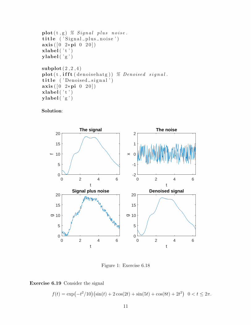
plot ( t , g ) % Signa l p l u s no i se .t i t l e ( ’ S i gna l p lus no i s e ’ )axis ( [ 0 2∗pi 0 2 0 ] )xlabel ( ’ t ’ )ylabel ( ’ g ’ )
subplot ( 2 , 2 , 4 )plot ( t , i f f t ( deno i sehatg ) ) % Denoised s i g n a l .t i t l e ( ’ Denoised s i g n a l ’ )axis ( [ 0 2∗pi 0 2 0 ] )xlabel ( ’ t ’ )ylabel ( ’ g ’ )
Solution:
0 2 4 6
t
0
5
10
15
20
f
The signal
0 2 4 6
t
-2
-1
0
1
2x
The noise
0 2 4 6
t
0
5
10
15
20
g
Signal plus noise
0 2 4 6
t
0
5
10
15
20
g
Denoised signal
Figure 1: Exercise 6.18
Exercise 6.19 Consider the signal
f(t) = exp(−t2/10
)(sin(t) + 2 cos(2t) + sin(5t) + cos(8t) + 2t2
)0 < t ≤ 2π.
11

Discretize f by setting fk = f(2kπ/256), k = 1, . . . , 256. Suppose the signal has beencorrupted by noise, modeled by the addition of the vector
x=2∗rand (1 ,2ˆ8)−0.5
Discretize f by setting fk = f(2kπ/256), k = 1, . . . , 256, as in Exercise 6.18. Thus theinformation in f is given by prescribing 256 ordered numbers, one for each value ofk. The problem here is to compress the information in the signal f by expressing itin terms of only 256c ordered numbers, where 0 < c < 1 is the compression ratio.This will involve throwing away some information about the original signal, but wewant to use the compressed data to reconstitute a facsimile of f that retains as muchinformation about f as possible. The strategy is to compute the FFT f of f andcompress the transformed signal by zeroing out the fraction 1 − c of the terms fkwith smallest absolute value. Apply the inverse FFT to the compressed transformedsignal to get a compressed signal fck . Plot the results and compare with the originaluncompressed signal. Experiment with several different values of c. A measure of theinformation lost from the original signal is L2error= ‖f − fc‖2 = ‖f‖2, so one wouldlike to have c as small as possible while at the same time keeping the L2 error as smallas possible. Experiment with c and with other signals, and also use your inspectionof the graphs of the original and compressed signals to judge the effectiveness of thecompression.
The following sample MATLAB program is an implementation of the compressionprocedure in Exercise 6.19.
% Input : time vec t o r t , s i g n a l v e c t o r f , compression ra t e c ,%( between 0 and 1)t=linspace (0 ,2∗pi , 2 ˆ 8 ) ;f=exp(−t . ˆ 2 / 1 0 ) .∗ ( sin ( t )+2∗cos (2∗ t)+sin (5∗ t)+cos (8∗ t )+2∗ t . ˆ 2 ) ;c =.5 ;ha t f=f f t ( f ) ;% Input v ec t o r f and r a t i o c : 0<= c <=1.% Output i s v e c t o r f c in which sma l l e s t% 100c% of terms f k , in a b s o l u t e va lue , are s e t% equa l to zero .N=length ( f ) ; Nc=f loor (N∗c ) ;f f=sort (abs ( hat f ) ) ;c u t o f f=abs ( f f (Nc+1)) ;
ha t f c =(abs ( hat f)>=c u t o f f ) . ∗ hat f ;f c= i f f t ( ha t f c ) ;L2error=norm( f−fc , 2 ) /norm( f ) ; %Re l a t i v e L2 in format ion l o s s
subplot ( 1 , 2 , 1 )plot ( t , f ) %Graph o f ft i t l e ( ’ Or i g i na l ’ )axis ( [ 0 2∗pi 0 9 ] )
12

xlabel ( ’ t ’ )ylabel ( ’ f ’ )
subplot ( 1 , 2 , 2 )plot ( t , fc , ’ r ’ ) % Graph o f compression o f ft i t l e ( [ ’ Compressed , c =0.5 , e r r=’ ,num2str( L2error ) ] )axis ( [ 0 2∗pi 0 9 ] )xlabel ( ’ t ’ )ylabel ( ’ f c ’ )
Solution:
0 1 2 3 4 5 6
t
0
1
2
3
4
5
6
7
8
9
f
Original
0 1 2 3 4 5 6
t
0
1
2
3
4
5
6
7
8
9
f c
Compressed, c=0.5, err=0.0067527
Figure 2: Exercise 6.19
13

Solutions to Chapter 7
Exercise 7.1 Verify that each of these four examples y(j)(n) defines a time-independent,causal, FIR filter, compute the associated impulse response vector h(j)(k) and deter-mine the number of taps.
Solution: y(1)(n) =∑∞
k=−∞ h(k)x(n−i), where h(k) = 0 except for h(1) = h(2) = 1/2.h(k) is independent of n, thus it is time-independent. h(k) = 0 for k < 0, thus it iscausal. h(k) 6= 0 for only finite k = 0, 1, thus it is FIR. The number of taps is 2.
y(2)(n) =∑∞
k=−∞ h(k)x(n − i), where h(k) = 0 except for h(0) = 1/2, h(1) = −1/2.h(k) is independent of n, thus it is time-independent. h(k) = 0 for k < 0, thus it iscausal. h(k) 6= 0 for only finite k = 0, 1, thus it is FIR. The number of taps is 2.
y(3)(n) =∑∞
k=−∞ h(k)x(n− i), where h(k) = 0 except for h(i) = 1/150, i = 0, . . . , 149.h(k) is independent of n, thus it is time-independent. h(k) = 0 for k < 0, thus it iscausal. h(k) 6= 0 for only finite k = 0, . . . , 149, thus it is FIR. The number of taps is150.
y(4)(n) =∑∞
k=−∞ h(k)x(n − i), where h(k) = 0 except for h(0) = 149/150, h(i) =−1/150, i = 1, . . . , 149. h(k) is independent of n, thus it is time-independent. h(k) = 0for k < 0, thus it is causal. h(k) 6= 0 for only finite k = 0, . . . , 149, thus it is FIR. Thenumber of taps is 150.
Exercise 7.2 Suppose the only nonzero components of the input vector x and the impulseresponse vector h are x0 = 1, x1 = 2 and h0 = 1/4, h1 = 1/2, h2 = 1/4. Compute theoutputs yn = (x ∗ h)n. Verify in the frequency domain that Y (ω) = H(ω)X(ω).
Solution: y0 = h0x0 = 1/4, y1 = x0h1 +x1h0 = 1, y2 = x0h2 +x1h1 = 5/4, y3 = x1h2 =1/2.
Y (ω) = 1/4 + e−iω + 5e−2iω/4 + e−3iω/2.
H(ω) = 1/4 + e−iω/2 + e−2iω/4.
X(ω) = 1 + 2e−iω
It is apparent to see that Y (ω) = H(ω)X(ω).
Exercise 7.3 Iterate the averaging filter H of Exercise 7.2 four times to get K = H4. Whatis K(ω) and what is the impulse response kn?
Solution: K(ω) = H4(ω) = 1/256 + e−iω/32 + 7e−2iω/64 + 7e−3iω/32 + 35e−4iω/128 +7e−5iω/32 + 7e−6iω/64 + e−7iω/32 + e−8iω/256.
Thus, k0 = 1/256, k1 = 1/32, k2 = 7/64, k3 = 7/32, k4 = 35/128, k5 = 7/32, k6 =7/64, k7 = 1/32, k8 = 1/256.
1

Exercise 7.4 Consider a filter with finite impulse response vector h. The problem is toverify the convolution rule Y = HX in the special case that h1 = 1 and all otherhn = 0. Thus
h = (. . . , 0, 0, 0, 1, 0, . . . ).
It will be accomplished in the following steps:
1. What is y = h ∗ x = h ∗ (. . . , x−1, x0, x1, . . . )?
2. What is H(ω)?
3. Verify that∑
yne−inω agrees with H(ω)X(ω).
Solution: 1. yk = xk−1.
2. H(ω) = e−iω.
3. Y (ω) =∑
k xke−i(k+1)ω, and X(ω) =
∑k xke
−ikω. Thus, it is easy to see thatY (ω) = H(ω)X(ω).
Exercise 7.5 • Write down the infinite matrix (↓ 3) that executes the downsampling:(↓ 3)xn = x3n.
• Write down the infinite matrix (↑ 3) that executes the upsampling:
(↑ 3)yn =
y
n3 , if 3 divides n
0, otherwise.
• Multiply the matrices (↑ 3)(↓ 3) and (↓ 3)(↑ 3). Describe the output for each ofthese product operations.
Solution:
(↓ 3) =
. . . . . .. . . 1 0 0 0 0 0 0 . . .. . . 0 0 0 1 0 0 0 . . .. . . 0 0 0 0 0 0 1 . . .. . . . . .
.
(↑ 3) =
. . . . . .
. . . 1 0 0 . . .
. . . 0 0 0 . . .
. . . 0 0 0 . . .
. . . 0 1 0 . . .
. . . 0 0 0 . . .
. . . 0 0 0 . . .
. . . 0 0 1 . . .
. . . . . .
.
2
(↑ 3)(↓ 3) =
. . . . . .
. . . 1 0 0 0 0 0 0 . . .
. . . 0 0 0 0 0 0 0 . . .
. . . 0 0 0 0 0 0 0 . . .
. . . 0 0 0 1 0 0 0 . . .
. . . 0 0 0 0 0 0 0 . . .
. . . 0 0 0 0 0 0 0 . . .
. . . 0 0 0 0 0 0 1 . . .
. . . . . .
.
(↓ 3)(↑ 3) = I.
Exercise 7.6 Show that if x ∈ `1 then x ∈ `2.
Solution: If x ∈ `1, then∞∑
k=−∞
|xk| <∞.
Thus, we have∞∑
k=−∞
|xk|2 ≤
(∞∑
k=−∞
|xk|
)2
<∞,
which indicates x ∈ `2.
Exercise 7.7 Verify the property (7.4) for the Z transform of the composition of two FIRfilters.
Solution: Since the Z transform of y = Φx = h ∗ y is Y [z] = H[z]X[z], and the Ztransform of w = Ψy = k ∗ y is W [z] = K[z]Y [z], thus W [z] = K[z]H[z]X[z], which isthe Z transform of w = Ψ(Φx) = k ∗ (h ∗ x).
Exercise 7.8 For each of the operators R,L, (↓ 2), (↑ 2),A,F,AIF determine which of theproperties of time invariance, causality and finite impulse response are satisfied.
Solution: R: time invariance, causality, finite impulse response.
L: time invariance, non-causality, finite impulse response.
(↓ 2): time invariance, non-causality, infinite impulse response.
(↑ 2): time invariance, non-causality, infinite impulse response.
AIF: time-dependent, non-causality, infinite impulse response.
Exercise 7.9 A direct approach to the convolution rule Y = HX. What is the coefficientof z−n in
(∑hkz
−k)(∑x`z−`)? Show that your answer agree with
∑hkxn−k.
Solution: The coefficient of z−n in(∑
hkz−k)(∑x`z
−`) is
a =∑
k+`=n
hkx` =∑k
hkxn−k.
3

Exercise 7.10 Let H be a causal filter with six taps, i.e., only coefficients h0, h1, . . . , h5
can be nonzero. We say that such a filter is anti-symmetric if the reflection of habout its midpoint (5/2 in this case) takes h to its negative: hk = −h5−k. Can such anantisymmetric filter ever be low pass? Either give an example or show that no exampleexists.
Solution: No, it cannot be a low pass filter. Since hk = −h5−k, we have H(0) =∑5k=0 hk = 0.
4

Solutions to Chapter 8
Exercise 8.1 Show directly that PP∗ = I on V ′.
Solution: Let φ ∈ V ′. Using (8.6), (8.7), (8.8) we have
PP∗φ = P
(∫ 1
0
φ(x1, y)dy
)=
e2πix2∑n=−∞
∫ 1
0
φ(n+ x1, y)dy
=∞∑
n=−∞
e2πinx2∫ 1
0
e−2πinyφ(x1, y)dy = φ(x1, x2),
so PP∗ = I on V ′.
Exercise 8.2 Using the results of Exercise 4.15, show that the Shannon-Whittaker samplingprocedure can be interpreted to define a tight frame. What is the frame bound?
Solution: Let the inner product be (f, g) =∫∞−∞ f(t) ¯g(t)dt and f (j)(t) = δ(t− πj
B), a
Dirac delta function. From Exercise 4.15 we have
‖f‖2 =π
B
∑j
|(f, f (j))|2,
so f (j) is a tight frame with frame bound B/π.
Exercise 8.3 Using the definition (8.22) of T∗ show that if ‖T‖ ≤ K for some constant Kthen ‖T∗‖ ≤ K. Hint: Choose f = T∗ξ.
Solution: Let f = T∗ξ, then
‖T∗ξ‖2 = (T∗ξ,T∗ξ)
=< ξ,TT∗ξ >
≤ ‖ξ‖ · ‖TT∗ξ‖≤ ‖ξ‖2 · ‖TT∗‖,
thus‖T∗ξ‖2
‖ξ‖2≤ ‖TT∗‖ ≤ ‖T‖ · ‖T∗‖,
which means‖T∗‖2 ≤ ‖T‖ · ‖T∗‖.
Therefore, we have‖T∗‖ ≤ ‖T‖ ≤ K.
1

Exercise 8.4 Verify that the requirement∫∞∞ w(t)dt = 0 ensure that C is finite, where
C =∫|w(λ)|2 dλ|λ| in the Plancherel formula for continuous wavelets.
Solution: If C is finite, we must have∫ 0
−ε
|w(λ)|2
|λ|dλ <∞ and
∫ ε
0
|w(λ)|2
|λ|dλ <∞,
where ε is an arbitrary positive real number and ε → 0+. If w(0) 6= 0, we can alwaysfind positive real number a and b such that∫ 0
−ε
|w(λ)|2
|λ|dλ > a
∫ 0
−ε
1
|λ|dλ→∞ and
∫ ε
0
|w(λ)|2
|λ|dλ > b
∫ ε
0
1
|λ|dλ→∞,
Thus, w(0) =∫∞∞ w(t)e−0tdt =
∫∞∞ w(t)dt must be zero to ensure C to be finite. Here,
we only prove that∫∞∞ w(t)dt = 0 is the necessary condition for C being finite.
Exercise 8.5 Consider the Haar mother wavelet
w(t) =
−1, 0 ≤ t < 1
2
1, 12≤ t < 1
0, otherwise.
Compute the explicit expression for the wavelet transform. Find the explicit integralexpression for C. Can you determine its exact value?
Solution: The continuous wavelet transform is
Fw(a, b) = |a|−1/2(∫ b+|a|/2
b
−f(t)dt+
∫ b+|a|
b+|a|/2f(t)dt
)
= |a|1/2(∫ 1/2
0
−f(au+ b)du+
∫ 1
1/2
f(au+ b)du
).
Since
w(λ) =
∫ ∞−∞
w(t)e−iλtdt =
∫ 1/2
0
−e−iλtdt+
∫ 1
1/2
e−iλtdt
=i− 2ie−iλ/2 + ie−iλ
λ
= −4sin2(λ/4)(sin(λ/2) + i cos(λ/2))
λ,
we have
|w(λ)|2 = w(λ) ∗ w(λ) =16 sin4(λ/4)
λ2.
Therefore
C =
∫ ∞∞
|w(λ)|2
|λ|dλ = 2
∫ ∞0
16 sin4(λ/4)
λ3dλ = 2 ln 2
2

Exercise 8.6 Show that the derivatives of the Gaussian distribution
w(n)(t) = Kndn
dtnG(t), G(t) =
1√2πσ
exp(−t2/2σ2
), n = 1, 2, . . .
each satisfy the conditions for reconstruction with a single wavelet in the case a > 0,provided the constant Kn is chosen so that ‖w(n)‖ = 1. In common use is the casen = 2, the Mexican hat wavelet. Graph this wavelet to explain the name.
Solution: Sincew(n)(λ) = Kn(iλ)n exp
(−σ2λ2
),
we have w(n)(0) ≡ 0 to satisfy the conditions for reconstruction with a single wavelet.For n = 2,
w(2)(t) =K2√2πσ5
(t2 − σ2) exp(−t2/2σ2
).
If ‖w(2)‖ = 1, we should have K2 = −(2/3)√
6π1/4σ5/2. Let σ = 1, then we have
w(2)(t) =2√
3
3π−1/4(1− t2) exp
(−t2/2
).
The plot of w(2)(t) is shown in Figure 1, whose shape is similar to a Mexican hat.
Exercise 8.7 Show that the continuous wavelets w(n) are insensitive to signals tk of orderk < n. Of course, polynomials are not square integrable on the real line. However, itfollows from this that w(n) will filter out most of the polynomial portion (of order < n)of a signal restricted to a finite interval.
Solution: Let’s prove it by induction. Obviously,∫∞−∞ w
(n)(t)dt =∫∞−∞w
(n)(t)dt = 0.Assume that for certain n ≥ 1, we have
Fn,k(a, b) = |a|1/2∫ ∞−∞
(at+ b)kw(n)(t)dt = 0, for 0 ≤ k < n.
Thus,
Fn+1,k(a, b) = |a|1/2∫ ∞−∞
(at+ b)kw(n+1)(t)dt (1 ≤ k < n+ 1)
= |a|1/2∫ ∞−∞
(at+ b)kd(w(n)(t)
)= |a|1/2
((at+ b)kw(n)(t)
∣∣∣∞−∞− ak
∫ ∞−∞
(at+ b)k−1w(n)(t)dt
).
Since w(n)(t) has the form of Pn(t)e−t2/2σ2
, where P (t) is a n-th polynomial respected
to t, we always have (at+ b)kw(n)(t)∣∣∣∞−∞
= 0 for the first part. Furthermore,∫∞−∞(at+
b)k−1w(n)(t)dt = 0 is obtained by the assumption. Hence, we prove that Fn+1,k(a, b) = 0for 0 ≤ k < n+ 1.
3

-5 -4 -3 -2 -1 0 1 2 3 4 5
t
-0.4
-0.2
0
0.2
0.4
0.6
0.8
1w
(t)
Figure 1: Exercise 8.6
Exercise 8.8 For students with access to the MATLAB wavelet toolbox. The MATLABfunction cwt computes F (a, b), (called Ca,b by MATLAB) for a specified discrete setof values of a and for b ranging the length of the signal vector. Consider the signalf(t) = e−t
2/10(sin t+ 2 cos 2t+ sin(5t+ cos 8t+ 2t22), 0 ≤ t < 2π. Discretize the signalinto a 512 component vector and use the Mexican hat wavelet gau2 to compute thecontinuous wavelet transform Ca,b for a taking integer values from 1 to 32 A simplecode that works is
t=linspace (0 ,2∗pi , 2 ˆ 8 ) ;f=exp(−t . ˆ 2 / 1 0 ) .∗ ( sin ( t )+2∗cos (2∗ t)+sin (5∗ t)+cos (8∗ t )+2∗ t . ˆ 2 ) ;c=cwt ( f , 1 : 3 2 , ’ gau2 ’ )
For color graphical output an appropriate command is
cc=cwt ( f , 1 : 3 2 , ’ gau2 ’ , ’ p l o t ’ )
This produces four colored graphs whose colors represent the magnitudes of the realand the imaginary parts of Ca,b, the absolute value of Ca,b and the phase angle ofCa,b, respectively, for the matrix of values (a, b). Repeat the analysis for the Haar
4

wavelet ′db1′ or ′haar′ and for ′cgau3′. Taking Exercise 8.7 into account, what is yourinterpretation of the information about the signal obtained from these graphs?
Solution: The above Matlab command can only work with the wavelet ′cgau3′ inMatlab of newer versions. The output is shown in Figure 2. Those graphs indicatethat the signal has weak oscillation in high frequency regime (a→ 1.0), but noticeableoscillation in intermediate and low frequency regimes (a→ 32.0).
Real part
50 100 150 200 250
Time b
1.00
5.00
9.00
13.00
17.00
21.00
25.00
29.00
Sca
les
a
Imaginary part
50 100 150 200 250
Time b
1.00
5.00
9.00
13.00
17.00
21.00
25.00
29.00
Sca
les
a
Modulus
50 100 150 200 250
Time b
1.00
5.00
9.00
13.00
17.00
21.00
25.00
29.00
Sca
les
a
Angle
50 100 150 200 250
Time b
1.00
5.00
9.00
13.00
17.00
21.00
25.00
29.00
Sca
les
a
Figure 2: The output with ‘cgau3′ wavelet of Exercise 8.8.
Exercise 8.9 Show that the affine translations w(a,b)(t) span L2(R) where w(t) = G(t), theGaussian distribution.
Solution: If f(t) ∈ L2(R) and 〈f, w(a,b)〉 = 0 for all a > 0 and b ∈ R. According to
5

Plancherel theorem, we have∫ ∞−∞
f(t)w(a,b)(t)dt =1
2π
∫ ∞−∞
f(λ)w(a,b)(λ)dλ
=1
2π
∫ ∞−∞
af(λ)e−(aσλ)2/2eibλdλ ≡ 0,
where the RHS is the inverse Fourier transform of af(λ)e−(aσλ)2/2 respected to b.
Due to the uniqueness of Fourier/inverse Fourier transform, we can conclude thataf(λ)e−(aσλ)
2/2 ≡ 0 and therefore f(λ) ≡ 0. Consequently, f(t) ≡ 0, which meansw(a,b)(t) span L2(R).
Exercise 8.10 Show that the set of affine translations of a complex Gaussian w(n)ω (t) span
L2(R). Hint: We already know that the affine translations of the real Gaussian (8.45)span L2(R).
Solution: Similar to Exercise 8.9, if f(t) ∈ L2(R) and 〈f,(w
(n)ω
)(a,b)〉 = 0 for all a > 0
and b ∈ R. According to Plancherel theorem, we have∫ ∞−∞
f(t)(w
(n)ω
)(a,b)(t)dt =
1
2π
∫ ∞−∞
f(λ)(w
(n)ω
)(a,b)(λ)dλ
=1
2π
∫ ∞−∞
af(λ)e−σ2(ω−aλ)2/2(iλ)neibλdλ ≡ 0,
where the RHS is the inverse Fourier transform of af(λ)e−σ2(ω−aλ)2/2(iλ)n respected to
b. Due to the uniqueness of Fourier/inverse Fourier transform, we can conclude thataf(λ)e−σ
2(ω−aλ)2/2(iλ)n ≡ 0 and therefore f(λ) ≡ 0. Consequently, f(t) ≡ 0, which
means(w
(n)ω
)(a,b)(t) span L2(R).
Exercise 8.11 This is a continuation of Exercise 8.5 on the Haar mother wavelet. Choosingthe lattice a0 = 2j, b0 = 1, for fixed integer j 6= 0, show that the discrete wavelets wmn
for m,n = 0,±1,±2, . . . form an ON set in L2(R). (In fact it is an ON basis.)
Solution: If the discrete wavelets wmn for m,n = 0,±1,±2, . . . based on Haar motherwavelet form an ON set in L2(R), the Haar mother wavelet should be defined in theinternal (0, 1] as
w(t) =
1, 1
2≤ t < 1
−1, 0 ≤ t < 12
0, otherwise.
Thus,
(wmn, wmn) = (2−mj/2)2∫ (n+1/2)2mj
n2mjdt+ (2−mj/2)2
∫ (n+1)2mj
(n+1/2)2mjdt =
1
2+
1
2= 1.
6

For m 6= m′ or n 6= n′, wmn and wm′n′
are either have non-overlapping domains ofdefinition, or the domain of definition of wmn (wm
′n′) is completely encompassed in
either arm of the domain of definition of wm′n′
(wmn). Therefore,(wmn, wm
′n′)≡ 0, for m 6= m′ or n 6= n′.
Exercise 8.12 For lattice parameters a0 = 2, b0 = 1, choose w+ = χ[1,2) and w− = χ(−2,−1].Show that w+ generates a tight frame for H+ with A = B = 1 and w− generates a tightframe for H− with A = B = 1, so wmn+ , wmn− is a tight frame for L2(R). (Indeed, onecan verify directly that wmn± is an ON basis for L2(R).)
Solution: For any integer m′ and any 1 ≤ ν < 2, we can have a ω = ν/(2m′2π) > 0
which is ranged in (0,∞], such that 1 ≤ am′2πω = 2m
′2πω < 2, and it is obvious that
am′−12πω < 1 and am
′+12πω ≥ 2. Thus∑m
|Fw+(am0 ω)|2 =∑m
|w+(am0 2πω)|2
= . . . 0 + 0 + 1 + 0 + 0 . . .
= 1
According to Lemma 8.21, wmn+ is a tight frame for H+ with A = B = 1/b0 = 1.Similarly, we can show that wmn− is a tight frame for H− with A = B = 1/b0 = 1.Hence, wmn+ , wmn− is a tight frame for L2(R).
Exercise 8.13 Let w be the function such that
Fw(ω) =1√ln a
0, if ω ≤ `
sin π2v(
ω−``(a−1)
), if ` < ω ≤ a`
cos π2v(
ω−a`a`(a−1)
), if a` < ω ≤ a2`
0, if ω > a2`
where v(x) is defined as in (8.27). Show that Fw(ω) is a tight frame for H+ withA = B = 1/b ln a. Furthermore, for w+ = w and w− = w show that wmn± is a tightframe for L2(R).
Solution: For any ω > 0, there must be certain m′ such that ` < am′ω ≤ a`. Let
ω′ = am′`, then∑
m
|Fw(amω)|2 = . . . 0 + 0 +1
ln asin2 π
2v
(ω′ − ``(a− 1)
)+
1
ln acos2
π
2v
(aω′ − a`a`(a− 1)
)+ 0 + 0 . . .
=1
ln a
(sin2 π
2v
(ω′ − ``(a− 1)
)+ cos2
π
2v
(ω′ − ``(a− 1)
))=
1
ln a.
7

According to Lemma 8.21, wmn is a tight frame for H+ with A = B = 1/b ln a.For w− = w, we have Fw−(ω) = Fw(−ω) = Fw(−ω), which has the support in theinterval [−a2`,−`]. Thus, wmn− is a tight frame for H− with A = B = 1/b ln a.Consequently, wmn± is a tight frame for L2(R).
Exercise 8.14 Verify formulas (8.2), using the definitions (8.3).
Solution: ∫ ∞−∞
t|g[x1,x2](t)|2dt =
∫ ∞−∞
t|e2πitx2g(t+ x1)|2dt
=
∫ ∞−∞
t|g(t+ x1)|2dt
=
∫ ∞−∞
(r − x1)|g(r)|2dr
=
∫ ∞−∞
r|g(r)|2dr − x1∫ ∞−∞|g(r)|2dr
= t0 − x1∫ ∞−∞
ω|g[x1,x2](ω)|2dω =
∫ ∞−∞
ω|F[e2πitx2g(t+ x1)
]|2dω
=
∫ ∞−∞
ω|e2πiωx1 g(t− x2)|2dt
=
∫ ∞−∞
(ν + x2)|g(ν)|2dν
=
∫ ∞−∞
ν|g(ν)|2dν + x2
∫ ∞−∞|g(ν)|2dν
= w0 + x2
Exercise 8.15 Derive the inequality (8.5).
Solution: Since g(ω) = g(2πω) and ‖g‖2 = ‖g‖2 = 12π‖g‖2 = 1, we have∫ ∞
−∞(t− t0)2|g(t)|2dt
∫ ∞−∞
(ω − ω0)2|g(ω)|2dω =
∫ ∞−∞
(t− t0)2|g(t)|2
‖g‖2dt
∫ ∞−∞
(ω − ω0)22π|g(2πω)|2
‖g‖2dω
= (Dt0g)
∫ ∞−∞
(λ
2π− ω0)
22π|g(λ)|2
‖g‖2dλ
2π
=1
4π2(Dt0g)
∫ ∞−∞
(λ− 2πω0)2 g(λ)|2
‖g‖2dλ
=1
4π2(Dt0g)(D2πω0 g).
The Heisenberg’s inequality ensures that
(Dt0g)(D2πω0 g) ≥ 1
4,
8

thus ∫ ∞−∞
(t− t0)2|g(t)|2dt∫ ∞−∞
(ω − ω0)2|g(ω)|2dω ≥ 1
16π2.
Exercise 8.16 Given the function
g(t) = φ(t) =
1, 0 ≤ t < 10, otherwise,
i.e., the Haar scaling function, show that the set g[m,n] is an ON basis for L2(R).Here, m,n run over the integers. Thus g[x1,x2] is overcomplete.
Solution: Since g[m,n](t) = e2πitng(t+m), we have(g[m,n], g[m
′,n′])
=
∫[−m,−m+1]∪[−m′,−m′+1]
e2πit(n−n′)g(t+m)g(t+m′)dt.
If m = m′ and n = n′,(g[m,n], g[m
′,n′])
= 1;
If m 6= m′, g(t+m)g(t+m′) ≡ 0 and therefore(g[m,n], g[m
′,n′])
= 0;
If m = m′ and n 6= n′,(g[m,n], g[m
′,n′])
=∫ 1
0e2πit(n−n
′)dt = 0.
Hence, the set g[m,n] is an ON basis for L2(R).
Exercise 8.17 Verify expansion (8.19) for a frame.
Solution: According to the definition of T∗, we have
(T∗ξ, f) =< ξ,Tf >=∑j
ξj(f, f (j)) =∑j
ξj(f(j), f) =
(∑j
ξjf(j), f
).
Thus, T∗ξ =∑
j ξjf(j).
Exercise 8.18 Show that the necessary and sufficient condition for a frame f (1), . . . , f (M)
in the finite-dimensional inner product space Vn is that the N ×M matrix Ω, (8.21),be of rank N . In particular we must have M ≥ N .
Solution: The condition that f (j) be a frame is that there exist real numbers 0 <A ≤ B such that
Aφtrφ ≤ φtrΩΩ∗φ ≤ Bφtrφ,
for all N -tuples φ.
Let λ1 ≥ λ2 ≥ · · · ≥ λN ≥ 0 be the N eigenvalues of ΩΩ∗. Apparently, A ≤ λN andB ≥ λ1. If such 0 < A ≤ B exists, we have λN ≥ A > 0, which means rank(ΩΩ∗) = Nand therefore rank(Ω) = N .
Conversely, if rank(Ω) = N , then we have rank(ΩΩ∗) = N and consequently λN > 0.Therefore, there exist real numbers A,B with 0 < A ≤ λN ≤ λ1 ≤ B such that
Aφtrφ ≤ φtrΩΩ∗φ ≤ Bφtrφ,
for all N -tuples φ, which means that f (j) is a frame.
9

Exercise 8.19 Show that the necessary and sufficient condition for a frame f (1), . . . , f (M)
in the finite-dimensional inner product space Vn to be a Riesz basis is that M = N .
Solution: According to Exercise 8.18, the necessary and sufficient condition for aframe f (1), . . . , f (M) in the finite-dimensional inner product space Vn is that the N×Mmatrix Ω be of rank N . In addition, to be a Riesz basis, f (1), . . . , f (M) must be linearlyindependent. Therefore, the necessary and sufficient condition for a frame f (1), . . . , f (M)
to be a Riesz basis is rank(Ω) = N and M = N .
Exercise 8.20 Show that the N ×M matrix defining the dual frame is (ΩΩ∗)−1Ω.
Solution: According to the definition of dual frame S−1f (j), where S = T∗T = ΩΩ∗,it is obviously that the dual frame is (ΩΩ∗)−1Ω.
Exercise 8.21 Verify that λj = σ2j , for j = 1, . . . , N where the σj are the singular values of
the matrix Ω, (8.21). Thus optimal values for A and B can be computed directly fromthe singular value decomposition of Ω.
Solution: Let UΣV ∗ = Ω be the singular value decomposition of Ω, where Σ =diag[σ1, σ2, . . . , σN ]. Therefore, UΣ2U∗ = ΩΩ∗ is the eigenvalue decomposition of ΩΩ∗,where Σ2 = diag[σ2
1, σ22, . . . , σ
2N ] = diag[λ1, λ2, . . . , λN ]. Hence, λj = σ2
j , for j =1, . . . , N .
Exercise 8.22 Show that expansion (8.21) for a frame in the finite-dimensional real innerproduct space VN corresponds to the matrix identity φ = ΩΩ∗(ΩΩ∗)−1φ
Solution: don’t know what exactly does the question mean.
Exercise 8.23 Find the matrix identity corresponding to the expansion (8.21) for a framein the finite-dimensional real inner product space VN .
Solution: don’t know what exactly does the question mean.
Exercise 8.24 By translation in t if necessary, assume that∫∞−∞ t|w±(t)|2dt = 0. Let
k+ =
∫ ∞0
y|Fw+(y)|2dy, k− =
∫ 0
−∞y|Fw−(y)|2dy.
Then w± are centered about the origin in position space and about k± in momentumspace. Show that∫ ∞
−∞t|w(a,b)± (t)|2dt = −b, ±
∫ ∞0
y|Fw(a,b)± (±y)|2dy = a−1k±,
so that w(a,b)± are centered about −b in time and a−1k± in frequency.
10

Solution: Since w(a,b)(t) = |a|−1/2w(t−ba
), thus∫ ∞
−∞t|w(a,b)± (t)|2dt =
∫ ∞−∞
t∣∣|a|−1/2w±(
t− ba
)∣∣2dt
=
∫ ∞−∞
(au+ b)
a
∣∣w±(u)∣∣2adu
= a
∫ ∞−∞
u∣∣w±(u)
∣∣2du+ b
∫ ∞−∞
∣∣w±(u)∣∣2du
= b.
Moreover, Fw(a,b)(y) = e−2πiby|a|1/2Fw(ay), thus
±∫ ∞0
y|Fw(a,b)± (±y)|2dy = ±
∫ ∞0
ay|Fw±(±ay)|2dy
= ±∫ ∞0
z|Fw±(±z)|2dza
= a−1k±.
Exercise 8.25 Show that if the support of w+ is contained in an interval of length ` in
the time domain then the support of w(a,b)+ is contained in an interval of length |a|l.
Similarly, show that if the support of Fw+ is contained in an interval of length L in
the frequency domain then the support of Fw(a,b)+ is contained in an interval of length
|a|−1L. This implies that the length and width of the “window” in time-frequencyspace will be rescaled by a and a−1 but the area of the window will remain unchanged.
Solution: Since w(a,b)(t) = |a|−1/2w(t−ba
)and Fw(a,b)(y) = e−2πiby|a|1/2Fw(ay), it is
obvious that there intervals are rescaled by |a| and |a|−1, respectively.
11

Solutions to Chapter 10
Exercise 10.1 For each of the Figures 10.1, 10.2, 10.3, determine the significance of thehorizontal and vertical scales
Solution: For Figure 10.1, 10.2 and 10.3, the horizontal scales can be mapped tothe support internal [0, 3], [0, 5] and [0, 7] for D4, D6 and D8. The vertical scales areadjusted according to the number of discretized points of the Daubechies wavelets inthe support internals, so that the norm of the vectors for the wavelets’ values is unit.
Exercise 10.2 Apply the cascade algorithm to the inner product vector of the ith iterateof the cascade algorithm with the scaling function itself
b(i)k =
∫ ∞−∞
φ(t)φ(i)(t− k)dt,
and derive, by the method leading to (10.1), the result
b(i+1) = Tb(i).
Solution:
b(i+1)s =
∫ ∞−∞
φ(t)φ(i+1)(t− s)dt =
∫ ∞−∞
φ(t+ s)φ(i+1)(t)dt
= 2∑k,`
c`ck
∫ ∞−∞
φ(2t+ 2s− `)φ(i)(2t− k)dt
=∑k,`
c`ck
∫ ∞−∞
φ(t+ 2s− `)φ(i)(t− k)dt
=∑k,`
c`ckb(i)2s−`+k =
∑m,j
c2s+mcm+jb(i)j ,
thusb(i+1) = Tb(i) = (↓ 2)CCtrb(i).
Exercise 10.3 The application of Theorem 10.1 to the Haar scaling function leads to anidentity for the sinc function. Derive it.
Solution: If φ(t) is the Haar scaling function, then φ(t) = e−iω/2sinc (ω/(2π)) and wehave the identity
A(ω) =∞∑
n=−∞
∣∣∣sinc( ω
2π+ n)∣∣∣2 =
∞∑n=−∞
∣∣∣∣sin(ω/2 + nπ)
ω/2 + nπ
∣∣∣∣2 ≡ 1.
1

Exercise 10.4 The finite T matrix for the dilation equation associated with a prospectivefamily of wavelets has the form
T =
0 − 1
160 0 0
1 916
0 − 116
00 9
161 9
160
0 − 116
0 916
10 0 0 − 1
160
Designate the components of the low pass filter defining this matrix by c0, . . . , cN .
1. What is N in this case? Give a reason for your answer.
2. The vector ak =∫φ(t)φ(t− k)dt, for k = −2,−1, 0, 1, 2 is an eigenvector of the
T matrix with eigenvalue 1. By looking at T can you tell if these wavelets areON?
3. The Jordan canonical form for T is
J =
1 0 0 0 00 1
20 0 0
0 0 18
0 00 0 0 1
41
0 0 0 0 14
What are the eigenvalues of T?
4. Does the cascade algorithm converge in this case to give an L2 scaling functionφ(t)? Give a reason for your answer.
5. What polynomials P (t) can be expanded by the φ(t − k) basis, with no error.(This is equivalent to determining the value of p.) Give a reason for your answer.
Solution: [−1/16, 0, 9/16, 1, 9/16, 0,−1/16] are the coefficients of the halfband filter
P [z] for the Daubechies wavelet D4. Thus, c0 = 1+√3
4√2, c1 = 3+
√3
4√2, c2 = 3−
√3
4√2, c3 = 1−
√3
4√2
.
1. The dimension of T is 2N − 1 = 5, so N = 3.
2. These wavelets are ON because for P [z] = − 116z3 + 9
16z+1+ 9
16z−1− 1
16z−3, P [z]+
P [−z] = 2.
3. The eigenvalues of T are 1, 12, 14
and 18.
4. Yes, because T has all its eigenvalues |λ| < 1 except for the simple eigenvalueλ = 1.
5. Any polynomial with order p ≤ 2 can be expanded by the φ(t− k) basis with noerror, since N = 2p− 1 = 5 and therefore p = 2.
2

Solutions to Chapter 11
Exercise 11.1 Verify that the 2-spline scaling function φ2(t) can be embedded in a 5/3filter bank defined by
S(0)[z] =
(1 + z−1
2
)2
, H(0)[z] =
(1 + z−1
2
)2
[−1 + 4z−1 − z−2],
i.e. p = 2 This corresponds to Daubechies D4 (which would be 4/4). Work out the filtercoefficients for the analysis and synthesis filters. Show that the convergence criteriaare satisfied, so that this defines a family of biorthogonal wavelets.
Solution: The synthesis filter coefficient is s0 = 14, s1 = 1
2, s2 = 1
4.
The analysis filter coefficient is h0 = −14, h1 = 1
2, h2 = 3
2, h3 = 1
2, h4 = −1
4.
Its halfband filter is P (0)[z] = S(0)[z]H(0)[z] = − 116z3 + 9
16z + 1 + 9
16z−1 − 1
16z−3. Thus
its finite T matrix is
T =
0 − 1
160 0 0
1 916
0 − 116
00 9
161 9
160
0 − 116
0 916
10 0 0 − 1
160
and its eigenvalues are 1, 1
2, 1
4, 1
8, which satisfies the convergence criteria of Theorem
10.2.
Exercise 11.2 Verify Lemma 11.14.
Solution: Since (↑M) means up sampling by M times, by definition we have
xk =
y k
M, if M divides k
0, otherwise
In frequency domain, as Y (ω) =∑
k yke−jkω, we haveX(ω)
∑k xke
−jkω =∑
k yke−jkMω =
Y (Mω).
For the Z transform, as Y [z] =∑
k ykz−k, we have X[z] =
∑k xkz
−k =∑
k ykz−Mk =
Y [zM ].
For u = (↓M)(↑M)x, as
1
M
M−1∑k=0
X[ze2πik/M ] =∑n
xn
(∑M−1k=0 e−2πikn/M
)M
z−n,
whereM−1∑k=0
e−2πikn/M =
M, if M divides n0, otherwise
1

Therefore,
1
M
M−1∑k=0
X[ze2πik/M ] =∑k
xkMz−kM ,
which is a subset of X[z] only taking the n-th term when M divides n.
Exercise 11.3 Let x = (x0, x1, x2, x3) be a finite signal. Write down the infinite signalsobtained from x by (a) zero padding, (b) constant padding with c = 1, (c) wraparound,(d) whole-point refection, (e) halfpoint refection.
Solution: (a)
xk =
xk, 0 ≤ k ≤ 30, otherwise
.
(b)
xk =
xk, 0 ≤ k ≤ 31, otherwise
.
(c)xn = xn mod 3.
(d)xn = xn mod 6, where x4 = x2, x5 = x1.
(e)xn = xn mod 8, where x4 = x3, x5 = x2, x6 = x1, x7 = x0.
Exercise 11.4 Verify explicitly that the circulant matrix Φ of Example 11.18 is diagonal inthe DFT frequency space and compute its diagonal elements.
Solution:
DΦ = F−1ΦF =1
MFΦF =
11 0 0 00 −3 0 00 0 −2− 3i 00 0 0 −2 + 3i
.
2

Solutions to Chapter 12
Exercise 12.1 Consider the image immediately above. Use a contrast stretch to constructthis image from the image
5 8 8 60 0 0 07 9 9 60 0 0 0
Solution: By using
b[m,n] =234(a[m,n]−min[a(m,n)])
max[a(m,n)]−min[a(m,n)],
we have
b =
130 208 208 1560 0 0 0
182 234 234 1560 0 0 0
.Exercise 11.2 Assume we have a system producing a dynamic range of 256, i.e., 8 bits
and the system adds two percent (of the dynamic range) random noise to the image.Suppose we measure the dark image first and then add two percent random noise to itas shown. Show that the contrast stretching has no effect on the dynamic range/noiseratio.
Solution: Since Inoise = Isignal+noise − Isignal and the stretching operator is
I ′[m,n] =(2N − 1)(I[m,n]−min[I(m,n)])
max[I(m,n)]−min[I(m,n)],
we have
I ′singal+noise[m,n] =(2N − 1)(Isingal[m,n]
max(Isignal+nosie)−min(Isignal+nosie)δ(Inoise)
Exercise 12.3 Consider the examples already studied. For a suitable structuring element Kof your choice, calculate (1) The boundary of the element below using the structuringelement shown. (2) The boundary of the nuts and bolts example using a dilation of 2.(3) Study the thickened boundary (AdK) ∩ (AeK). What do you find?
1

Solution: (1) Let
A =
0 0 0 0 0 0 00 0 0 1 0 0 00 0 1 1 1 0 00 1 1 1 1 1 00 0 1 1 1 0 00 0 0 1 0 0 00 0 0 0 0 0 0
, K =
1 1 11 1 11 1 1
then the boundary of A is
∂A =
0 0 0 0 0 0 00 0 0 1 0 0 00 0 1 0 1 0 00 1 0 0 0 1 00 0 1 0 1 0 00 0 0 1 0 0 00 0 0 0 0 0 0
.
The thickened boundary (AdK) ∩ (AcdK) is
(AdK) ∩ (AcdK) =
0 0 0 1 0 0 00 0 1 1 1 0 00 1 1 0 1 1 01 1 0 0 0 1 10 1 1 0 1 1 00 0 1 1 1 0 00 0 0 1 0 0 0
.
Exercise 12.4 Apply the skeletal algorithm above to the nuts and bolts example above.
Solution: For another picture with circles, the comparison of the original and skele-tonized pictures is shown in Figure 1.
Exercise 12.5 Take FTs of two images. Add them using a suitable morphology operatorfor example a blend, and take the inverse Fourier Transform of the sum. Explain theresult.
Solution: Two pictures for blending is shown in Figure 2. The blended picture isshown in Figure 3.
Exercise 12.6 Add different sorts of noise to two images and compare the FT’s. Investigateif the Fourier Transform is distributive over multiplication.
Solution:
2
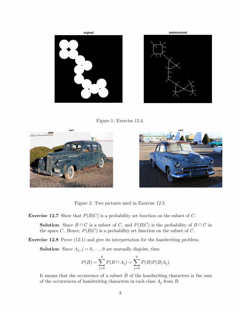
orginal skeletonized
Figure 1: Exercise 12.4.
car1 car2
Figure 2: Two pictures used in Exercise 12.5.
Exercise 12.7 Show that P (B|C) is a probability set function on the subset of C.
Solution: Since B ∩ C is a subset of C, and P (B|C) is the probability of B ∩ C inthe space C. Hence, P (B|C) is a probability set function on the subset of C.
Exercise 12.8 Prove (12.1) and give its interpretation for the handwriting problem.
Solution: Since Aj, j = 0, . . . , 9 are mutually disjoint, thus
P (B) =9∑j=0
P (B ∩ Aj) =9∑j=0
P (B)P (B|Aj).
It means that the occurrence of a subset B of the handwriting characters is the sumof the occurrences of handwriting characters in each class Aj from B.
3

blended
Figure 3: Blended picture for Exercise 12.5.
Exercise 12.9 Suppose the set of training vectors is such that a = 1, c = 5 in the proof ofTheorem 12.6 and we start the Perceptron algorithm with w(1) as the zero n+ 1-tuple.Find the smallest k such that the algorithm is guaranteed to terminate in at most ksteps.
Solution: If a = 1, c = 5 and w(1) = 0, ‖z′‖′ = 1, we have
k2 ≤
∥∥∥∥∥k∑j=1
x′(j)
∥∥∥∥∥2
≤k∑j=1
‖x′(j)‖2 ≤ 5k.
Thusk2 − 5k ≤ 0 ⇒ k ≤ 5.
There,the algorithm is guaranteed to terminate in approximately 5 steps.
Exercise 12.10 Find an example in two dimensions and an example in three dimensions ofClass 1 and Class 2 training vectors that are not linearly separable.
Solution: In two dimension
Class 1 =v = (x, y) | x2 + y2 < r2
, Class 2 =
v = (x, y) | x2 + y2 > r2
,
is not linearly separable.
In three dimension
Class 1 =v = (x, y, z) | x2 + y2 + z2 < r2
, Class 2 =
v = (x, y, z) | x2 + y2 + z2 > r2
,
is not linearly separable.
4

Exercise 12.11 Show that E(CS) = C, i.e., the expectation of CS is C.
Solution:
E(CSi,j
)= E
(1
n− 1
m∑k=1
(T
(k)i − Ti
)(T
(k)j − Tj
))
=1
n− 1
m∑k=1
(T
(k)i − E(Ti)
)(T
(k)j − E(Tj)
)= E[(Ti − E(Ti))(Tj − E(Tj))] = Ci,j
Exercise 12.12 Verify the following properties of the n × n sample covariance matrix CS
and the n ×m matrix (12.6). (1) CS = XtrX, (2) (CS)tr = CS. (3) The eigenvaluesλj of CS are nonnegative.
Solution: (1) Since
CSi,j =
1
n− 1
m∑k=1
(T
(k)i − Ti
)(T
(k)j − Tj
)=
m∑k=1
1√n− 1
(T
(k)i − Ti
) 1√n− 1
(T
(k)j − Tj
)=
m∑k=1
Xk,iXk,j,
thus CS = XtrX.
(2) As CSi,j = CS
j,i ⇒ (CS)tr = CS.
(3) for any z ∈ Rn, z 6= 0, we have
ztrCSz = ztrXtrXz = ‖Xz‖2 ≥ 0,
therefore CS is semi-definite positive, i.e. the eigenvalues λj of CS are nonnegative.
Exercise 12.1(1) Take each of the examples below, with 16 pixels and 3 bit dynamic rangemonochrome values and apply a contrast stretch and histogram normalization. Whatwould you expect to see in real images of these types?
(A) :
0 1 1 10 2 1 61 1 6 56 7 7 7
, (B) :
7 6 5 46 7 5 55 5 6 74 5 7 6
(C) :
2 3 2 33 2 3 53 6 5 66 5 6 5
5

(2) Suppose that in a binary image you have k white pixels in a total of N pixels. Findthe mean and variance of the image.
(3) (a) Show that the mean of an image with dynamic range of n bits is 1/2(2n − 1)if histogram normalization has been applied to it. (b) Write down a formula for thevariance of the images in (a). (c) What is the implication of (a)-(b) for contrast andbrightness?
Solution: (1) The results of stretching (A), (B), (C) are0 1 1 10 2 1 61 1 6 56 7 7 7
,
7 5 2 00 7 1 62 2 5 70 2 7 5
,
0 2 0 22 0 2 52 7 5 77 5 7 5
.Nothing has change in (A). The contrast of (B) and (C) has been enhanced.
(2)
mean =k
N, variance =
1
N − 1
(k
(1− k
N
)2
+ (N − k)
(k
N
)2)
=k(N − k)
N(N − 1).
(3) Problem??
Exercise 12.2 (a) Consider each of the three images below. Each is the Fourier transformof an image. Roughly sketch the original image
(A) :
space space space· · ·
space space space
, (B) :
space · space spacespace space space spacespace · space space
(C) :
space space space space space· space space · ·
space space space space space
(b) Suppose we take an image which consists of spaces everywhere except on thediagonal where it has a high pixel value. What will its Fourier transform look like?Explain your answer.
Solution: (a)
(A) : |F−1(∗)| =
a b ca b ca b c
, (B) : |F−1(∗)| =
a a a ab b b bc c c c
(C) : |F−1(∗)| =
a b c d ea b c d ea b c d e
6

(b) The Fourier transform of a squared diagonal graph looks like
|F(∗)| =
∗
∗∗
∗∗
which has its dominate values along the −1st anti-diagonal and the upper-left corner.This is because the 2D DFT for squared diagonal graph x is
X = WxW,
where W is the conjugate of the Fourier transform matrix. If x has large values alongits diagonal, then
X ≈ cW 2,
where c is a large positive real number. Since W is symmetric unitary, and its columnhas the relationship wn = e2π(n−1)i/Nw1, the dominate entries of X should be Xm,n
wheremod (m+ n− 2, N) = 0.
Since 1 ≤ m,n ≤ N , thus m+ n = N + 2 or m = n = 1.
Exercise 12.13 Gray scale morphology operators: (a) Show that the following is true: if fis the intensity function for an image and k is a hemisphere structuring function then
• fdk = T [U [f ]dU [k]].
• fek = T [U [f ]eU [k]].
• fok = T [U [f ]oU [k]].
• fck = T [U [f ]cU [k]].
(b) Prove the Umbra Homomorphism Theorem:
• U [fdg] = U [f ]dU [g].
• U [feg] = U [f ]eU [g].
• U [fog] = U [feg]dU [g] = U [f ]oU [g].
Solution: (a) T [U [f ]dU [k]] = T [f ]dTU [k] = fdk.
T [U [f ]eU [k]] = TU [f ]eTU [k] = fek.
T [U [f ]oU [k]] = TU [f ]oTU [k] = fok.
T [U [f ]cU [k]] = TU [f ]cTU [k] = fck.
(b) U [fdg] = U [T [f ]dT [g]] = UT [f ]dUT [g] = U [f ]dU [g].
U [feg] = U [T [f ]eT [g]] = UT [f ]eUT [g] = U [f ]eU [g].
U [fog] = U [(feg)dg] = U [feg]dU [g] = (U [f ]eU [g])dU [g] = U [f ]oU [g].
7

Exercise 12.14 Find the opening and closing of the images (A)–(C) in Exercise 254 forsuitable structuring elements of your choice.
Solution: Exercise 254?
Exercise 12.15 Prove that if A and B are umbras, then so is AdB.
Solution: if A and B are umbras, we have
AdB = UT (A)dUT (B) = U [T (A)dT (B)].
Thus, AdB is an umbra.
Exercise 12.16 Consider an image with pixels over [0, 4]. The gray scale function for theimage intensity is given by f(x) = x− 1 for 1 ≤ x ≤ 2, f(x) = 3− x for 2 ≤ x ≤ 3 and0 elsewhere. The structuring function is a hemisphere of radius 0.25, i.e.,
k(x) =√
0.0625− x2, −0.25 ≤ x ≤ 0.25.
Find the opening and closing of f by k and discuss what this should do to the visualaspects of the image.
Solution: The shapes of feg, fdg, fcg, fog are shown in Figure 4 and Figure 5.
0 0.5 1 1.5 2 2.5 3 3.5 40
0.1
0.2
0.3
0.4
0.5
0.6
0.7f e g
0 0.5 1 1.5 2 2.5 3 3.5 40
0.2
0.4
0.6
0.8
1
1.2
1.4f d g
Figure 4: feg and fdg for Exercise 12.16.
Exercise 12.17 Write a program to implement the 3×3 skeletonization algorithm describedabove and try it out on some images
Solution:
8

0 0.5 1 1.5 2 2.5 3 3.5 40
0.1
0.2
0.3
0.4
0.5
0.6
0.7
0.8
0.9f o g
0 0.5 1 1.5 2 2.5 3 3.5 40
0.1
0.2
0.3
0.4
0.5
0.6
0.7
0.8
0.9
1f c g
Figure 5: fog and fcg for Exercise 12.16.
BW1 = imread ( ’ c ircbw . t i f ’ ) ;BW2 = bwmorph(BW1, ’ s k e l ’ , Inf ) ;f iguresubplot ( 1 , 2 , 1 )imshow (BW1)t i t l e ( ’ o r g i n a l ’ )subplot ( 1 , 2 , 2 )imshow (BW2)t i t l e ( ’ s k e l e t o n i z e d ’ )
orginal skeletonized
Figure 6: Exercise 12.17.
9

Exercise 12.18 Consider the pattern classes (0, 0), (0, 1) and (1, 0), (1, 1). Use thesepatterns to train a perceptron algorithm to separate patterns into two classes aroundthese. [Do not forget to augment the patterns and start with zero weights.]
Solution: Let w(0) = (0, 0, 0), x1 = (0, 0, 1), x2 = (0, 1, 1), x3 = (1, 0, 1), x4 = (1, 1, 1);Class 1 requires (w,−xi) > 0 and Class 1 requires (w, xi) > 0.
(w(0),−x1) = 0⇒ w(1) = w(0) − w1 = (0, 0,−1);
(w(1),−x2) = −1 < 0⇒ w(2) = w(1) − w2 = (0,−1,−2);
(w(2), x3) = −2 < 0⇒ w(3) = w(2) + w3 = (1,−1,−1);
(w(3), x4) = −1 < 0⇒ w(4) = w(3) + w4 = (2, 0, 0);
(w(4),−x1) = 0⇒ w(5) = w(4) − w1 = (2, 0,−1);
(w(5),−x2) = 1 > 0;
(w(5), x3) = 1 > 0;
(w(5), x4) = 1 > 0;
Thus, the hyperplane for separating the two classes is 2x− 1 = 0.
Exercise 12.19 Suppose we have a collection of pattern classes and in each case the dis-tribution of the patterns around the cluster center is Gaussian. Suppose also thatthe pattern components are uncorrelated. [This means the covariance matrix is theidentity.] Find a formula for the probability that a given pattern vector x belongs tocluster wj . In this case, given a pattern vector x, deduce that the decision as to whichclass it belongs to would be made simply on its distance to the nearest cluster center.
Solution: Since the distribution of each class is Gaussian and they are independent,the value of the probability density function (PDF) of each case for each class revealsthe chance of that case belonging to the indicated class Thus, we can assign patternvector x to cluster ωj with have the maximal PDF with assumed mean (center) amongall the clusters. Apparently, higher PDF indicates closer distance of the pattern vectorto the center of the cluster. Therefore, the decision of which class a x belonging towould be made on its distance to the nearest cluster center.
Exercise 12.20 Consider the following 20 two-dimensional vectors:
x =
(x1x2
):
(x1 = 4.1, 2.8, 0.5, 3.1, 4.8, 1.5, 3.8, 2.4, 1.7, 2.0, 0.2, 3.5, 2.1, 0.8, 2.9, 4.4, 3.7, 5, 4, 1.3)
(x2 = 9.7, 6.3, 2.4, 7.2, 10.2, 4.4, 9, 5.4, 4.7, 4.8, 1.5, 8, 5.7, 2.5, 6.7, 10, 8.8, 10.5, 9.3, 3.3)
Without using a MATLAB program, find its principal components and comment onthe results.
Solution: Since
x · xT =
(188.38 433.49433.39 1005..02
),
10

its eigen-polynomial isλ2 − 1193.40λ+ 1412.0875 = 0.
thus, its eigenvalues are
λ1 = 1192.216, λ2 = 1.1844,
and therefore its principle components is the eigenvector
v1 =
(0.3964470.918057
).
Since λ1 λ2, the distribution of xi, i = 1, . . . , 20 is dominated along v1 direction.
Exercise 12.21 In this chapter, we have given a self-contained introduction to some tech-niques dealing with the parsimonious representation of data. MATLAB offers severaltoolboxes which allow one to implement demos on data. Study the imaging and sta-tistical pattern toolbox demos given in the links:
http://cmp.felk.cvut.cz/cmp/software/stprtool/examples.html
http://www-rohan.sdsu.edu/doc/matlab/toolbox/images/images.html
Solution:
11