solar neutrino measurements in super … a measurement of this oscillation parameter. it is also...

Solar neutrino measurements in Super-Kamiokande-IV

K. Abe,1,32 Y. Haga,1 Y. Hayato,1,32 M. Ikeda,1 K. Iyogi,1 J. Kameda,1,32 Y. Kishimoto,1,32 Ll. Marti,1 M. Miura,1,32

S. Moriyama,1,32 M. Nakahata,1,32 T. Nakajima,1 S. Nakayama,1,32 A. Orii,1 H. Sekiya,1,32 M. Shiozawa,1,32 Y. Sonoda,1

A. Takeda,1,32 H. Tanaka,1 Y. Takenaga,1 S. Tasaka,1 T. Tomura,1 K. Ueno,1 T. Yokozawa,1 R. Akutsu,2 T. Irvine,2 H. Kaji,2

T. Kajita,2,32 I. Kametani,2 K. Kaneyuki,2,32,* K. P. Lee,2 Y. Nishimura,2 T. McLachlan,2 K. Okumura,2,32 E. Richard,2

L. Labarga,3 P. Fernandez,3 F. d. M. Blaszczyk,4 J. Gustafson,4 C. Kachulis,4 E. Kearns,4,32 J. L. Raaf,4 J. L. Stone,4,32

L. R. Sulak,4 S. Berkman,5 S. Tobayama,5 M. Goldhaber,6,* K. Bays,7 G. Carminati,7 N. J. Griskevich,7 W. R. Kropp,7

S. Mine,7 A. Renshaw,7 M. B. Smy,7,32 H. W. Sobel,7,32 V. Takhistov,7 P. Weatherly,7 K. S. Ganezer,8 B. L. Hartfiel,8 J. Hill,8

W. E. Keig,8 N. Hong,9 J. Y. Kim,9 I. T. Lim,9 R. G. Park,9 T. Akiri,10 J. B. Albert,10 A. Himmel,10 Z. Li,10 E. O’Sullivan,10

K. Scholberg,10,32 C. W. Walter,10,32 T. Wongjirad,10 T. Ishizuka,11 T. Nakamura,12 J. S. Jang,13 K. Choi,14 J. G. Learned,14

S. Matsuno,14 S. N. Smith,14 M. Friend,15 T. Hasegawa,15 T. Ishida,15 T. Ishii,15 T. Kobayashi,15 T. Nakadaira,15

K. Nakamura,15,32 K. Nishikawa,15 Y. Oyama,15 K. Sakashita,15 T. Sekiguchi,15 T. Tsukamoto,15 Y. Nakano,16

A. T. Suzuki,16 Y. Takeuchi,16,32 T. Yano,16 S. V. Cao,17 T. Hayashino,17 T. Hiraki,17 S. Hirota,17 K. Huang,17 K. Ieki,17

M. Jiang,17 T. Kikawa,17 A. Minamino,17 A. Murakami,17 T. Nakaya,17,32 N. D. Patel,17 K. Suzuki,17 S. Takahashi,17

R. A. Wendell,17,32 Y. Fukuda,18 Y. Itow,19,20 G. Mitsuka,19 F. Muto,19 T. Suzuki,19 P. Mijakowski,21 K. Frankiewicz,21

J. Hignight,22 J. Imber,22 C. K. Jung,22 X. Li,22 J. L. Palomino,22 G. Santucci,22 I. Taylor,22 C. Vilela,22 M. J. Wilking,22

C. Yanagisawa,22,† D. Fukuda,23 H. Ishino,23 T. Kayano,23 A. Kibayashi,23 Y. Koshio,23,32 T. Mori,23 M. Sakuda,23

J. Takeuchi,23 R. Yamaguchi,23 Y. Kuno,24 R. Tacik,25,34 S. B. Kim,26 H. Okazawa,27 Y. Choi,28 K. Ito,29 K. Nishijima,29

M. Koshiba,30 Y. Totsuka,30,* Y. Suda,31 M. Yokoyama,31,32 C. Bronner,32 R. G. Calland,32 M. Hartz,32 K. Martens,32

Y. Obayashi,32 Y. Suzuki,32 M. R. Vagins,32,7 C. M. Nantais,33 J. F. Martin,33 P. de Perio,33 H. A. Tanaka,33 A. Konaka,34

S. Chen,35 H. Sui,35 L. Wan,35 Z. Yang,35 H. Zhang,35 Y. Zhang,35 K. Connolly,36 M. Dziomba,36 and R. J. Wilkes36

(Super-Kamiokande Collaboration)

1Kamioka Observatory, Institute for Cosmic Ray Research, University of Tokyo,Kamioka, Gifu 506-1205, Japan

2Research Center for Cosmic Neutrinos, Institute for Cosmic Ray Research,University of Tokyo, Kashiwa, Chiba 277-8582, Japan

3Department of Theoretical Physics, University Autonoma Madrid, 28049 Madrid, Spain4Department of Physics, Boston University, Boston, Massachusetts 02215, USA

5Department of Physics and Astronomy, University of British Columbia,Vancouver, British Columbia V6T1Z4, Canada

6Physics Department, Brookhaven National Laboratory, Upton, New York 11973, USA7Department of Physics and Astronomy, University of California,

Irvine, Irvine, California 92697-4575, USA8Department of Physics, California State University, Dominguez Hills, Carson, California 90747, USA

9Department of Physics, Chonnam National University, Kwangju 500-757, Korea10Department of Physics, Duke University, Durham North Carolina 27708, USA

11Junior College, Fukuoka Institute of Technology, Fukuoka, Fukuoka 811-0295, Japan12Department of Physics, Gifu University, Gifu, Gifu 501-1193, Japan

13GIST College, Gwangju Institute of Science and Technology, Gwangju 500-712, Korea14Department of Physics and Astronomy, University of Hawaii, Honolulu, Hawaii 96822, USA15High Energy Accelerator Research Organization (KEK), Tsukuba, Ibaraki 305-0801, Japan

16Department of Physics, Kobe University, Kobe, Hyogo 657-8501, Japan17Department of Physics, Kyoto University, Kyoto, Kyoto 606-8502, Japan

18Department of Physics, Miyagi University of Education, Sendai, Miyagi 980-0845, Japan19Institute for Space-Earth Enviromental Research, Nagoya University, Nagoya, Aichi 464-8602, Japan

20Kobayashi-Maskawa Institute for the Origin of Particles and the Universe,Nagoya University, Nagoya, Aichi 464-8602, Japan

21National Centre For Nuclear Research, 00-681 Warsaw, Poland22Department of Physics and Astronomy, State University of New York at Stony Brook,

New York 11794-3800, USA23Department of Physics, Okayama University, Okayama, Okayama 700-8530, Japan

24Department of Physics, Osaka University, Toyonaka, Osaka 560-0043, Japan25Department of Physics, University of Regina, 3737 Wascana Parkway, Regina,

Saskatchewan S4SOA2, Canada

PHYSICAL REVIEW D 94, 052010 (2016)

2470-0010=2016=94(5)=052010(32) 052010-1 © 2016 American Physical Society

26Department of Physics, Seoul National University, Seoul 151-742, Korea27Department of Informatics in Social Welfare, Shizuoka University of Welfare,

Yaizu, Shizuoka, 425-8611, Japan28Department of Physics, Sungkyunkwan University, Suwon 440-746, Korea

29Department of Physics, Tokai University, Hiratsuka, Kanagawa 259-1292, Japan30The University of Tokyo, Bunkyo, Tokyo 113-0033, Japan

31Department of Physics, University of Tokyo, Bunkyo, Tokyo 113-0033, Japan32Kavli Institute for the Physics and Mathematics of the Universe (WPI), The University of Tokyo Institutes

for Advanced Study, University of Tokyo, Kashiwa, Chiba 277-8583, Japan33Department of Physics, University of Toronto, 60 St., Toronto, Ontario M5S1A7, Canada

34TRIUMF, 4004 Wesbrook Mall, Vancouver, British Columbia V6T2A3, Canada35Department of Engineering Physics, Tsinghua University, Beijing 100084, China

36Department of Physics, University of Washington, Seattle, Washington 98195-1560, USA(Received 23 June 2016; published 20 September 2016)

Upgraded electronics, improved water system dynamics, better calibration and analysis techniquesallowed Super-Kamiokande-IV to clearly observe very low-energy 8B solar neutrino interactions, withrecoil electron kinetic energies as low as ∼3.5 MeV. Super-Kamiokande-IV data-taking began inSeptember of 2008; this paper includes data until February 2014, a total livetime of 1664 days. Themeasured solar neutrino flux is ð2.308� 0.020ðstatÞþ0.039

−0.040 ðsystÞÞ × 106=ðcm2 secÞ assuming no oscil-lations. The observed recoil electron energy spectrum is consistent with no distortions due to neutrinooscillations. An extended maximum likelihood fit to the amplitude of the expected solar zenith anglevariation of the neutrino-electron elastic scattering rate in SK-IV results in a day/night asymmetry ofð−3.6� 1.6ðstatÞ � 0.6ðsystÞÞ%. The SK-IV solar neutrino data determine the solar mixing angle assin2θ12 ¼ 0.327þ0.026

−0.031 , all SK solar data (SK-I, SK-II, SK III and SK-IV) measures this angle to be

sin2θ12 ¼ 0.334þ0.027−0.023 , the determined mass-squared splitting is Δm2

21 ¼ 4.8þ1.5−0.8 × 10−5 eV2.

DOI: 10.1103/PhysRevD.94.052010

I. INTRODUCTION

Solar neutrino flux measurements from Super-Kamiokande (SK) [1] and the Sudbury NeutrinoObservatory (SNO) [2] have provided clear evidence forsolar neutrino flavor conversion in which electron flavorneutrinos convert to either muon or tau flavor neutrinos. Thisflavor conversion is well described by flavor oscillations ofthree neutrinos. In particular, the extracted oscillation param-eters agree with nuclear reactor antineutrino measurements[3]. However, while oscillations of reactor antineutrinos at thesolar frequency were observed, there is still no clear evidencethat the solar neutrino flavor conversion is indeed due toneutrino oscillations and not caused by another mechanism.Currently there are two types of testable signatures uniqueto neutrino oscillations, the first being the observationand precision test of the Mikheyev–Smirnov–Wolfenstein(MSW) resonance curve [4], the characteristic energydependence of the flavor conversion (assuming oscillationparameters extracted from solar neutrino and reactor anti-neutrino measurements): higher energy solar neutrinos(higher energy 8B and hep neutrinos) undergo adiabaticresonant conversion within the Sun (present data imply a

survival probability of about 30%), while the flavor changesof the lower energy solar neutrinos (pp, 7Be, pp, CNO andlower energy 8B neutrinos) arise only from vacuum oscil-lations. These averaged vacuum oscillations lead to anaverage survival probability which—for sufficiently small1–3 mixing—must exceed 50% (present data imply about60%). The transition from the matter-dominated oscillationswithin the Sun to the vacuum-dominated oscillations shouldoccur near three MeV. This makes 8B neutrinos the bestchoice when looking for a transition point within the energyspectrum. An observed deviation from the expected behaviorin the transition region would imply new physics, e.g.nonstandard interactions [5] or mass-varying neutrinos [6].A second signature unique to oscillations arises from theeffect of the terrestrial matter density on solar neutrinooscillations. This effect is tested directly by comparing solarneutrinos that pass long distances through the Earth atnighttime to those which do not pass through the Earthduring the daytime. Those neutrinos which pass through theEarth will generally have an enhanced electron neutrinocontent, leading to an increase in the nighttime electron elasticscattering rate (or any charged-current interaction rate), andhence a negative “day/night asymmetry” ðrD − rNÞ=rave,where rD (rN) is the daytime (nighttime) rate and rave ¼12ðrD þ rNÞ is the average rate. This day/night asymmetry

depends on the solar mass squared splitting and therefore

*Deceased.†Also at BMCC/CUNY, Science Department, New York,

New York, USA.

K. ABE et al. PHYSICAL REVIEW D 94, 052010 (2016)

052010-2

http://dx.doi.org/10.1103/PhysRevD.94.052010




constitutes a measurement of this oscillation parameter. It isalso sensitive to new physics. SK is sensitive to 8B and hepsolar neutrinos in the energy range around 4 to 18.7MeVandprecisely measures the neutrino interaction time. It is there-fore a good detector to search for both solar neutrinooscillation signatures.SK [7] is a large, cylindrical, water Cherenkov detector

containing 50,000 tons of ultrapure water. It is located1,000m beneath the peak ofMount Ikenoyama, in KamiokaTown, Japan. The SK detector is optically separated into a32.5 kton cylindrical inner detector (ID) surrounded by a∼2.5 meter water shield, ∼2 m of which is the active vetoouter detector (OD). The structure dividing the detectorregions contains an array of photomultiplier tubes (PMTs).SK started data-taking in April of 1996, with 11,146 ID and1,885ODPMTs, andwas then shut down formaintenance inJune of 2001. This period is called SK-I [1]. While refillingthe tank with water in November of 2001, a PMT implosioncaused a chain reaction which destroyed 60% of the PMTs.The surviving and new PMTs were redistributed andcovered with fiber-reinforced plastic (FRP) and acryliccases, in order to avoid another accidental chain reaction.Data-taking restarted with 5,182 ID and 1,885 OD PMTs inDecember of 2002, and the period until October of 2005 iscalled SK-II [8]. In October of 2006, newly manufacturedPMTs replaced those which had been destroyed, and with11,129 ID and 1,885 OD PMTs data-taking resumed as theSK-III phase [9]. The fourth phase of SK (SK-IV) began inSeptember of 2008, with new front-end electronics (QTCBasedElectronicswith Ethernet, QBEE [10]) for both the IDand OD, new data acquisition system, and continues to thisday. This paperwill include data taken up until the beginningof February 2014.Improvements in the front-end electronics, the water

circulation system, calibration techniques and the analysismethods have allowed the SK-IV solar neutrino measure-ments to be made with a lower energy threshold and smallersystematic uncertainties, compared to SK-I, II and III. Thehardware and software improvements are summarized inSec. II, while the SK-IV data set, data reduction, and itssystematic uncertainty estimations on the total flux aredetailed in Sec. III. The simulation of solar neutrino eventsin SK is described also in Sec. III. Unfortunately, thesimulation code for the SK-III period used in [9] wasinaccurate, which affected the input recoil electron spectrum.The details (and the correction applied) as well as a reanalysisof the SK-III data are briefly described in Sec. III andAppendix A.In Sec. IV, the energy spectrum results of SK-IVaswell as

all SK phases combined are discussed. Section V presentsthe SK-IV day/night asymmetry analysis. Finally, Sec. VIcontains an oscillation analysis of SK-IV data by themselvesand in combination with other SK phases, and also a globalanalysis which combines the SK results with other relevantexperiments.

In previous SK solar neutrino publications [1,8,9]“energy” meant total recoil electron energy, while in thispaper we subtract the electron mass me ¼ 511 keV toobtain kinetic energy. The kinetic energy threshold of theSK-IV data analysis is thus 3.49 MeV, corresponding to thetotal energy of 4.00 MeV.

II. DETECTOR PERFORMANCE

A. Electronics, data acquisition system

To ensure stable observation and to improve the sensi-tivity of the detector, new front-end electronics calledQBEEs were installed, allowing for the development ofa new online data acquisition system. The essentialcomponents on the QBEEs used for the analog signalprocessing and digitization are the QTC (high-speedcharge-to-time converter) ASICs [10], which achieve veryhigh speed signal processing and allow the integration ofthe charge and recording of the time of every PMT signal.These PMT signal times and charge integrals are sent toonline computers, where a software trigger searches fortiming coincidences within 200 ns to pick out events in asimilar fashion as the hardware “hitsum trigger” did in SK-Ithrough III [1,8,9]. The energy threshold of this coinci-dence trigger is determined by the number of coincidentPMT signals that are required: a smaller coincidence levelwill be more sensitive to lower energy events, but will resultin larger event rates. The definitions of the different triggertypes and the corresponding typical event rates are sum-marized in Table I. Since all PMT signals are digitized andrecorded, there is no deadtime of the detector from a largetrigger rate, so the efficiency of triggering on HE eventsdoes not limit the maximum possible rate of SLE triggers;only the processing capability of the online computerslimits this maximum rate. The software trigger system usesflexible event time periods (1.3 μ sec for SLE, 40 μ sec forLE and HE). The trigger efficiencies for the thresholds are∼84% (∼99%) between 3.49 and 3.99 MeV (3.99 and4.49 MeV) and 100% above 4.49 MeV.

B. Water system

To keep the long light attenuation length of the SK waterstable, the water is continuously purified with a flow rate of60 ton=hour. Purified water supplied to the bottom of thedetector replaces water drained from its top. A highertemperature of the supply water than the detector temperature

TABLE I. Normal data-taking trigger types along with thethreshold of hits and average trigger rates.

Trigger type Hits in 200 ns Trigger rate

Super low energy (SLE) 34 3.0–3.4 kHzLow energy (LE) 47 ∼40 HzHigh energy (HE) 50 ∼10 Hz

SOLAR NEUTRINO MEASUREMENTS IN SUPER- … PHYSICAL REVIEW D 94, 052010 (2016)

052010-3

results in convection throughout the detector volume. Thisconvection transports radioactive radon gas, which is pro-duced by radioactive decays from the U/Th chain near theedge of the detector into the central region of the detector.Radioactivity coming from the decay products of radon gas(most commonly 214Bi beta decays)mimics the lowest energysolar neutrino events. In January of 2010, a new automatedtemperature control systemwas installed, allowing for controlof the supply water temperature at the�0.01 degree level. Bycontrolling the water flow rate and the supply water temper-ature with such high precision, convection within the tank iskept to a minimum and the background level in the centralregion has since become significantly lower.

C. Event reconstruction

The methods used for the vertex, direction, and energyreconstructions are the same as those used for SK-III [9].The Cartesian coordinate system for the SK detector isshown in Fig. 1.

1. Vertex

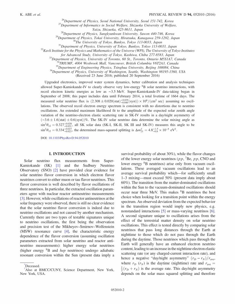
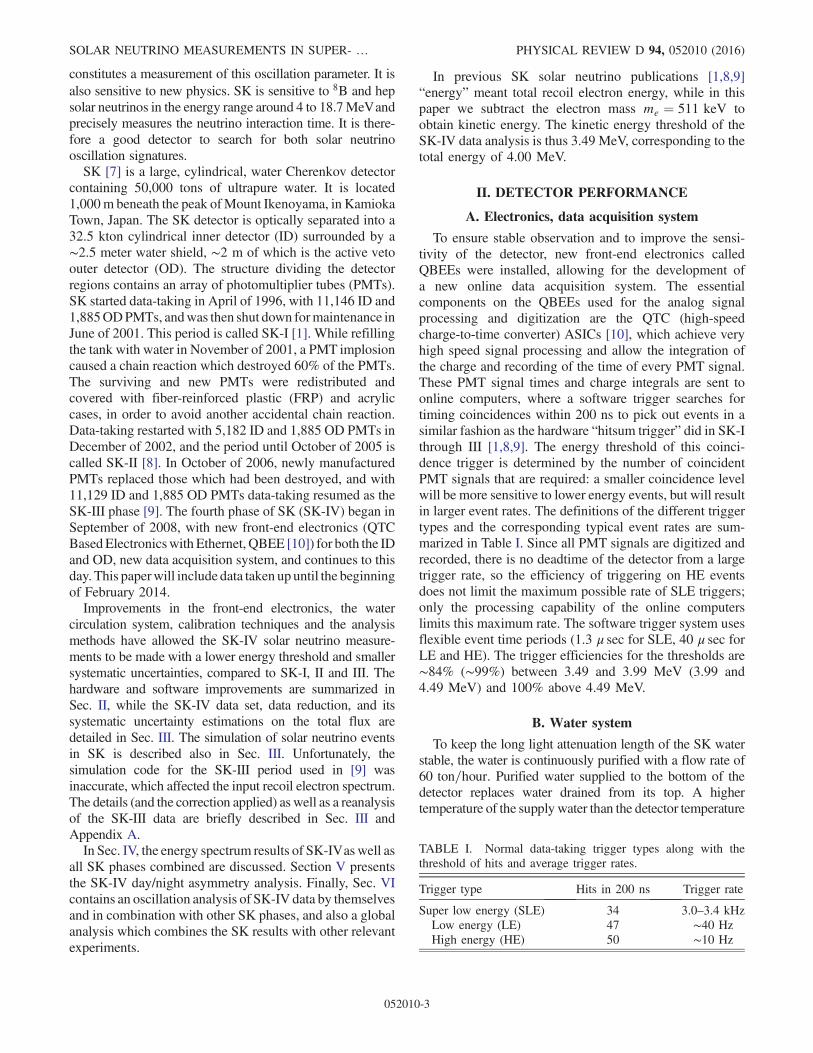
The vertex reconstruction is a maximum likelihood fit tothe arrival times of the Cherenkov light at the PMTs [8].Figure 2 shows the vertex resolution for each SK phase. Thelarge improvement in SK-III compared to SK-I is the result ofusing an advanced vertex reconstruction program, while theimproved timing resolution and slightly better agreement ofthe timing residuals between data and Monte Carlo (MC)simulated events are responsible for the additional improve-ment of SK-IV.Weobserved a bias in the reconstructed vertexcalled the vertex shift. This vertex shift is measured with agamma-ray source at several positionswithin the SKdetector:neutrons from spontaneous fission of 252Cf are thermalized inwater and then captured on nickel in a spherical vessel [7,11].The nickel then emits 9MeVgammas (Ni calibration source).Figure 3 shows the shift of the reconstructed vertex of theseNigammas in SK-IV from their true position (assumed to be thesource position). The SK-IV vertex shift is improved com-pared with SK-I, II, and III [7–9].

2. Direction

A maximum likelihood fit comparing the Cherenkovring pattern of data to MC simulations is used to reconstruct

event directions. During the SK-III phase an energydependence was included in the likelihood and the angularresolution was improved by about 10% (10 MeVelectrons)compared to SK-I. The angular resolution in SK-IV issimilar to that in SK-III.

3. Energy

The energy reconstruction is based on the number of PMThits within a 50 ns time window, after the photon travel timefrom the vertex is subtracted. This number is then correctedfor water transparency, dark noise, late arrival light (due toscattering and reflection),multiphoton hits, etc., producing aneffective number of hits Neff (see [9]). Simulations ofmonoenergetic electrons are used to produce a functionrelating Neff to the recoil electron energy (MeV).

FIG. 1. Definition of the SK detector coordinate system.

True Electron Energy (MeV)

Ver

tex

Res

olut

ion

(cm

)

0

50

100

150

200

250

5 7.5 10 12.5 15

FIG. 2. Vertex resolution for SK-I, II, III, and IV shown by thedotted, dashed-dotted, dashed, and solid lines, respectively. TheSK-III vertex resolution improvement over SK-I comes fromusing an improved vertex reconstruction while the slightlyimproved timing resolution and better agreement between dataand simulated events are responsible for the further improvementin SK-IV.

-10

0

10

0 5 10 15r (m)

z (m

)

10 cm

FIG. 3. Vertex shift of the Ni calibration events in SK-IV.The start of the arrow is at the true Ni-Cf source position and thedirection indicates the averaged vertex shift at that position. Thelength of the arrow indicates the magnitude of the vertex shift. Tomake the vertex shifts easier to see this length is scaled up by afactor of 20.


052010-4

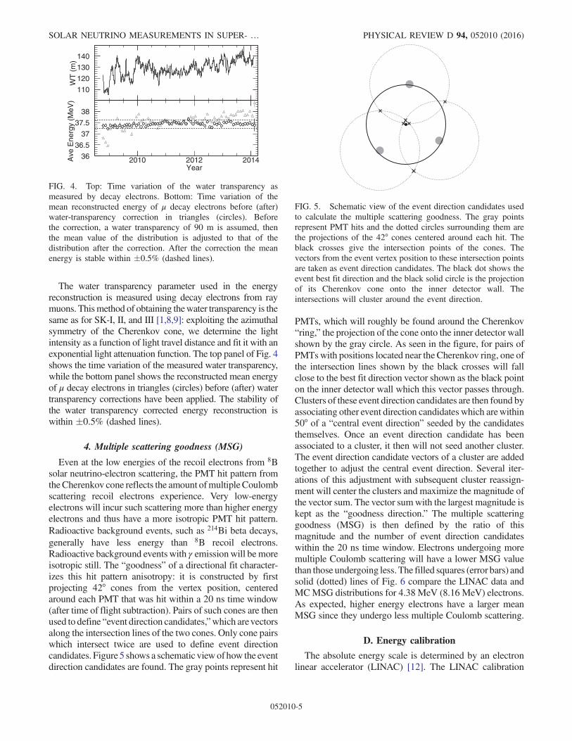
The water transparency parameter used in the energyreconstruction is measured using decay electrons from raymuons. Thismethod of obtaining thewater transparency is thesame as for SK-I, II, and III [1,8,9]: exploiting the azimuthalsymmetry of the Cherenkov cone, we determine the lightintensity as a function of light travel distance and fit it with anexponential light attenuation function. The top panel of Fig. 4shows the time variation of the measured water transparency,while the bottom panel shows the reconstructed mean energyof μ decay electrons in triangles (circles) before (after) watertransparency corrections have been applied. The stability ofthe water transparency corrected energy reconstruction iswithin �0.5% (dashed lines).

4. Multiple scattering goodness (MSG)

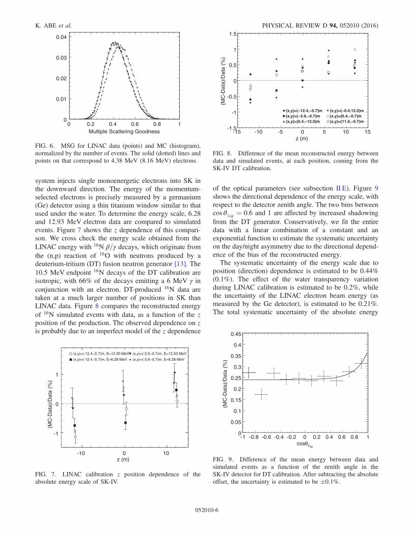
Even at the low energies of the recoil electrons from 8Bsolar neutrino-electron scattering, the PMT hit pattern fromtheCherenkov cone reflects the amount ofmultipleCoulombscattering recoil electrons experience. Very low-energyelectrons will incur such scattering more than higher energyelectrons and thus have a more isotropic PMT hit pattern.Radioactive background events, such as 214Bi beta decays,generally have less energy than 8B recoil electrons.Radioactive background events with γ emission will be moreisotropic still. The “goodness” of a directional fit character-izes this hit pattern anisotropy: it is constructed by firstprojecting 42° cones from the vertex position, centeredaround each PMT that was hit within a 20 ns time window(after time of flight subtraction). Pairs of such cones are thenused to define “event direction candidates,”which arevectorsalong the intersection lines of the two cones. Only cone pairswhich intersect twice are used to define event directioncandidates. Figure 5 shows a schematic viewof how the eventdirection candidates are found. The gray points represent hit

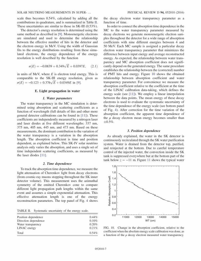
PMTs, which will roughly be found around the Cherenkov“ring,” the projection of the cone onto the inner detector wallshown by the gray circle. As seen in the figure, for pairs ofPMTswith positions located near the Cherenkov ring, one ofthe intersection lines shown by the black crosses will fallclose to the best fit direction vector shown as the black pointon the inner detector wall which this vector passes through.Clusters of these event direction candidates are then found byassociating other event direction candidates which arewithin50° of a “central event direction” seeded by the candidatesthemselves. Once an event direction candidate has beenassociated to a cluster, it then will not seed another cluster.The event direction candidate vectors of a cluster are addedtogether to adjust the central event direction. Several iter-ations of this adjustment with subsequent cluster reassign-ment will center the clusters and maximize the magnitude ofthe vector sum. The vector sumwith the largest magnitude iskept as the “goodness direction.” The multiple scatteringgoodness (MSG) is then defined by the ratio of thismagnitude and the number of event direction candidateswithin the 20 ns time window. Electrons undergoing moremultiple Coulomb scattering will have a lower MSG valuethan those undergoing less. The filled squares (error bars) andsolid (dotted) lines of Fig. 6 compare the LINAC data andMCMSG distributions for 4.38 MeV (8.16 MeV) electrons.As expected, higher energy electrons have a larger meanMSG since they undergo less multiple Coulomb scattering.

D. Energy calibration

The absolute energy scale is determined by an electronlinear accelerator (LINAC) [12]. The LINAC calibration

110

120

130

140

WT

(m

)

36

36.5

37

37.5

38

2010 2012 2014Year

Ave

Ene

rgy

(MeV

)

FIG. 4. Top: Time variation of the water transparency asmeasured by decay electrons. Bottom: Time variation of themean reconstructed energy of μ decay electrons before (after)water-transparency correction in triangles (circles). Beforethe correction, a water transparency of 90 m is assumed, thenthe mean value of the distribution is adjusted to that of thedistribution after the correction. After the correction the meanenergy is stable within �0.5% (dashed lines).

FIG. 5. Schematic view of the event direction candidates usedto calculate the multiple scattering goodness. The gray pointsrepresent PMT hits and the dotted circles surrounding them arethe projections of the 42° cones centered around each hit. Theblack crosses give the intersection points of the cones. Thevectors from the event vertex position to these intersection pointsare taken as event direction candidates. The black dot shows theevent best fit direction and the black solid circle is the projectionof its Cherenkov cone onto the inner detector wall. Theintersections will cluster around the event direction.


052010-5

system injects single monoenergetic electrons into SK inthe downward direction. The energy of the momentum-selected electrons is precisely measured by a germanium(Ge) detector using a thin titanium window similar to thatused under the water. To determine the energy scale, 6.28and 12.93 MeV electron data are compared to simulatedevents. Figure 7 shows the z dependence of this compari-son. We cross check the energy scale obtained from theLINAC energy with 16N β=γ decays, which originate fromthe (n,p) reaction of 16O with neutrons produced by adeuterium-tritium (DT) fusion neutron generator [13]. The10.5 MeV endpoint 16N decays of the DT calibration areisotropic, with 66% of the decays emitting a 6 MeV γ inconjunction with an electron. DT-produced 16N data aretaken at a much larger number of positions in SK thanLINAC data. Figure 8 compares the reconstructed energyof 16N simulated events with data, as a function of the zposition of the production. The observed dependence on zis probably due to an imperfect model of the z dependence

of the optical parameters (see subsection II E). Figure 9shows the directional dependence of the energy scale, withrespect to the detector zenith angle. The two bins betweencos θzSK ¼ 0.6 and 1 are affected by increased shadowingfrom the DT generator. Conservatively, we fit the entiredata with a linear combination of a constant and anexponential function to estimate the systematic uncertaintyon the day/night asymmetry due to the directional depend-ence of the bias of the reconstructed energy.The systematic uncertainty of the energy scale due to

position (direction) dependence is estimated to be 0.44%(0.1%). The effect of the water transparency variationduring LINAC calibration is estimated to be 0.2%, whilethe uncertainty of the LINAC electron beam energy (asmeasured by the Ge detector), is estimated to be 0.21%.The total systematic uncertainty of the absolute energy

Multiple Scattering Goodness

0

0.01

0.02

0.03

0.04

0 0.2 0.4 0.6 0.8 1

FIG. 6. MSG for LINAC data (points) and MC (histogram),normalized by the number of events. The solid (dotted) lines andpoints on that correspond to 4.38 MeV (8.16 MeV) electrons.

-1

0

1

-10 0 10

(x,y)=(-12.4,-0.7)m, E=12.93 MeV

(x,y)=(-12.4,-0.7)m, E=6.28 MeV

(x,y)=(-3.9,-0.7)m, E=12.93 MeV

(x,y)=(-3.9,-0.7)m, E=6.28 MeV

z (m)

(MC

-Dat

a)/D

ata

(%)

FIG. 7. LINAC calibration z position dependence of theabsolute energy scale of SK-IV.

z (m)-15 -10 -5 0 5 10 15

(MC

-Dat

a)/D

ata

(%)

-1.5

-1

-0.5

0

0.5

1

1.5

(x,y)=(−12.4,−0.7)m(x,y)=(−3.9,−0.7)m(x,y)=(0.4,−12.0)m

(x,y)=(−0.4,12.0)m(x,y)=(0.4,−0.7)m(x,y)=(11.0,−0.7)m

FIG. 8. Difference of the mean reconstructed energy betweendata and simulated events, at each position, coming from theSK-IV DT calibration.

SKzθcos-1 -0.8 -0.6 -0.4 -0.2 0 0.2 0.4 0.6 0.8 1

(MC

-Dat

a)/D

ata

(%)

0

0.05

0.1

0.15

0.2

0.25

0.3

0.35

0.4

0.45

FIG. 9. Difference of the mean energy between data andsimulated events as a function of the zenith angle in theSK-IV detector for DT calibration. After subtracting the absoluteoffset, the uncertainty is estimated to be �0.1%.


052010-6

scale thus becomes 0.54%, calculated by adding all thecontributions in quadrature, and is summarized in Table II.These uncertainties are similar to those in SK-III (0.53%).The detector’s energy resolution is determined using the

same method as described in [9]. Monoenergetic electronsare simulated and used to determine the relationshipbetween the effective number of hits in the detector andthe electron energy in MeV. Using the width of Gaussianfits to the energy distributions resulting from these simu-lated electrons, the energy dependence of the energyresolution is well described by the function

σðEÞ ¼ −0.0839þ 0.349ffiffiffiffiE

pþ 0.0397E; ð2:1Þ

in units of MeV, where E is electron total energy. This iscomparable to the SK-III energy resolution, given asσðEÞ ¼ −0.123þ 0.376

ffiffiffiffiE

p þ 0.0349E in [9].

E. Light propagation in water

1. Water parameters

The water transparency in the MC simulation is deter-mined using absorption and scattering coefficients as afunction of wavelength (full details of this and other moregeneral detector calibrations can be found in [11]). Thesecoefficients are independently measured by a nitrogen laserand laser diodes at five different wavelengths: 337 nm,375 nm, 405 nm, 445 nm, and 473 nm. Based on thesemeasurements, the dominant contribution to the variation ofthe water transparency is a variation in the absorptionlength. The absorption coefficient is time and positiondependent, as explained below. This SK-IV solar neutrinoanalysis only varies the absorption, and uses a single set oftime independent scattering coefficients, as measured bythe laser diodes [11].

2. Time dependence

To track the absorption time dependence, we measure thelight attenuation of Cherenkov light from decay electrons(from cosmic-ray muons stopping throughout the SK innerdetector volume). This measurement uses the azimuthalsymmetry of the emitted Cherenkov cone to comparedifferent light propagation path lengths within the sameevent and assumes a simple exponential attenuation. Thiseffective attenuation length is one of the energyreconstruction parameters. The top panel of Fig. 4 shows

the decay electron water transparency parameter as afunction of time.In order to connect the absorption time dependence in the

MC to the water transparency parameter measured bydecay electrons we generate monoenergetic electron sam-ples throughout the detector for a wide range of absorptioncoefficients with nine different energies between 4 and50 MeV. Each MC sample is assigned a particular decayelectron water transparency parameter that minimizes thedifference between input energy and average reconstructedenergy. As expected, the relationship between water trans-parency and MC absorption coefficient does not signifi-cantly depend on the generated energy. The same procedureestablishes the relationship between the (corrected) numberof PMT hits and energy. Figure 10 shows the obtainedrelationship between absorption coefficient and watertransparency parameter. For convenience we measure theabsorption coefficient relative to the coefficient at the timeof the LINAC calibration data-taking, which defines theenergy scale (see [11]). We employ a linear interpolationbetween the data points. The mean energy of these decayelectrons is used to evaluate the systematic uncertainty ofthe time dependence of the energy scale (see bottom panelof Fig. 4). After correction for the time variation of theabsorption coefficient, the apparent time dependence ofthe μ decay electron mean energy becomes smaller than�0.5%.

3. Position dependence

As already explained, the water in the SK detector iscontinuously recirculated through the SK water purificationsystem. Water is drained from the detector top, purified,and reinjected at the bottom. Due to careful temperaturecontrol of the injected water, the convection inside the SKtank is suppressed everywhere but at the bottom part of thetank below z ¼ −11 m. Figure 11 shows the typical water

TABLE II. Systematic uncertainty of the energy scale.

Position dependence 0.44%Direction dependence 0.10%Water transparency 0.20%LINAC energy 0.21%

Total 0.54%

WT (cm)11000 12000 13000 14000 15000

Rel

ativ

e A

bsor

ptio

n C

oeff.

0.2

0.4

0.6

0.8

1

1.2

1.4

1.6

1.8

FIG. 10. Change in the absorption coefficient, relative to thecoefficient when the absolute energy scale calibrationwas done, asa function of the μ decay electron measured water transparency.


052010-7

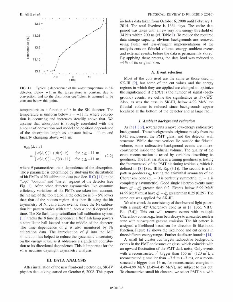
temperature as a function of z in the SK detector. Thetemperature is uniform below z ¼ −11 m, where convec-tion is occurring and increases steadily above that. Weassume that absorption is strongly correlated with theamount of convection and model the position dependenceof the absorption length as constant below −11 m andlinearly changing above −11 m:

αabsðλ; z; tÞ

¼�αðλ; tÞð1þ βðtÞ · zÞ; for z ≥ −11 m

αðλ; tÞð1 − βðtÞ · 11Þ; for z ≤ −11 m;ð2:2Þ

where β parametrizes the z-dependence of the absorption.The β parameter is determined by studying the distributionof hit PMTs of Ni calibration data (see Sec. II C) [11] in the“top,” “bottom,” and “barrel” regions of the detector (seeFig. 1). After other detector asymmetries like quantumefficiency variations of the PMTs are taken into account,the hit rate of the top region in the detector is 3 ∼ 5% lowerthan that of the bottom region. β is then fit using the hitasymmetry of Ni calibration events. Since the Ni calibra-tion hit pattern varies with time, both α and β depend ontime. The Xe flash lamp scintillator ball calibration system[11] tracks the β time dependence: a Xe flash lamp powersa scintillator ball located near the middle of the detector.The time dependence of β is also monitored by Nicalibration data. The introduction of β into the MCsimulation has helped to reduce the systematic uncertaintyon the energy scale, as it addresses a significant contribu-tion to its directional dependence. This is important for thesolar neutrino day/night asymmetry analysis.

III. DATA ANALYSIS

After installation of the new front-end electronics, SK-IVphysics data-taking started on October 6, 2008. This paper

includes data taken from October 6, 2008 until February 1,2014. The total livetime is 1664 days. The entire dataperiod was taken with a new very low energy threshold of34 hits within 200 ns (cf. Table I). To reduce the requireddata storage capacity, obvious backgrounds are removedusing faster and less-stringent implementations of theanalysis cuts on fiducial volume, energy, ambient eventsand external events, before the data is permanently stored.By applying these precuts, the data load was reduced to∼1% of its original size.

A. Event selection

Most of the cuts used are the same as those used inSK-III [9], but some of the cut values and the energyregions in which they are applied are changed to optimizethe significance: if S (BG) is the number of signal (back-ground) events, we define the significance as S=

ffiffiffiffiffiffiffiBG

p.

Also, as was the case in SK-III, below 4.99 MeV thefiducial volume is reduced since backgrounds appearlocalized at the bottom of the detector and at large radii.

1. Ambient background reduction

As in [1,8,9], several cuts remove low-energy radioactivebackgrounds. These backgrounds originate mostly from thePMT enclosures, the PMT glass, and the detector wallstructure. While the true vertices lie outside the fiducialvolume, some radioactive background events are misre-constructed inside the fiducial volume. The quality of theevent reconstruction is tested by variables describing itsgoodness. The first variable is a timing goodness gt testingthe “narrowness” of the PMT hit timing residuals, which isdefined in [8] [Sec. III B, Eq. (3.1)]. The second is a hitpattern goodness gp testing the azimuthal symmetry of theCherenkov cone (gp ¼ 0 is perfectly symmetric, gp ¼ 1 iscompletely asymmetric). Good single electron events musthave g2t − g2p greater than 0.2. Events below 6.99 MeV(4.99MeV) must have g2t − g2p greater than 0.25 (0.29). Thesame cut was applied for SK-III.We also check the consistency of the observed light pattern

with a single 42° Cherenkov cone as in [1] [Sec. VII C,Eq. (7.4)]. This cut will remove events with multipleCherenkov cones, e.g., from beta decays to an excited nuclearstate with subsequent gamma emission. The hit pattern isassigned a likelihood based on the direction fit likelihoodfunction. Figure 12 shows the likelihood and cut criteria inthree different energy ranges. Further details are found in [14].A small hit cluster cut targets radioactive background

events in the PMT enclosures or glass, which coincide withan upward fluctuation of the PMT dark noise. Only eventswith a reconstructed r2 bigger than 155 m2 (120 m2), areconstructed z smaller than −7.5 m (−3 m), or a recon-structed z bigger than 13 m, for reconstructed energies in4.49–4.99 MeV (3.49–4.49 MeV), are subject to this cut.To characterize small hit clusters, we select PMT hits with

13.1

13.15

13.2

13.25

13.3

-10 0 10z (m)

Tem

pera

ture

(o C

)

FIG. 11. Typical z dependence of the water temperature in SKdetector. Below −11 m the temperature is constant due toconvection, and so the absorption coefficient is assumed to beconstant below this point.


052010-8

times coincident within 20 ns (after time-of-flight sub-traction, see Sec. II C 3), and then find the smallest spherearound any of the selected PMTs that encloses at least 20%of all selected PMTs. This radius is multiplied by the ratioof PMT hits coincident within 20 ns (without time-of-flightcorrection) divided byNeff (see Sec. II C 3). Solar neutrinosnear the edge of the fiducial volume have a bigger radius ×hit ratio (see also Sec. III C in [9], Fig. 17 and 18) than theradioactive background. As in SK-III, we remove eventswith radius × hit ratio less than 75 cm as shown in Fig. 12.Finally, we remove spurious events due to various cali-

bration sources (mostly radioactive decays), if they are below

4.99 MeV. A reconstructed position closer than 2 m to thesource, or closer than 1 m to the source or water temperaturesensor cable (all cables run along the z axis from the top downto the source position)means the event is removed. The loss inthe fiducial volume is about 0.48 kton. Table III lists thevarious calibration sources which are considered.

2. External event cut

To remove radioactive background coming from thePMTs or the detector wall structure, we calculate thedistance to the PMT-bearing surface from the reconstructedvertex looking back along the reconstructed event direction.Radioactive backgrounds tend to appear “incoming,” so weremove events where this distance is small. Solar neutrinocandidates above 7.49 MeV (above 4.99 MeV and below7.49 MeV) must have a distance of at least 4 m (6.5 m). Inthe energy region below 4.99 MeV we distinguish betweenthe “top” (cylinder top lid), “barrel” (cylinder side walls)and “bottom” (cylinder bottom lid) surfaces, shown inFig. 1. Candidates which come from the “top” (“bottom”)must have a distance of at least 10 m (13 m), while “barrel”event candidate distances must exceed 12 m. SK-III appliedthe same cuts.

TABLE III. Locations used by the calibration source cut. Thesources are described in detail in [11].

Source x (cm) y (cm) z (cm)

Xenon flasher 353.5 −70.7 0.0LED 35.5 −350.0 150.0TQ Diffuser Ball −176.8 −70.7 100.0DAQ Rate Test Source −35.3 353.5 100.0Water Temp. Sensors 1 −35.3 1200 −2000Water Temp. Sensors 2 70.7 −777.7 −2000

radius [cm]0 200 400 600 800 1000 1200 1400

0.1

0.2

0.3

0.4

0.5

0.6

0.7

0.8

0

5000

10000

15000

20000

25000Data

0.2

0.3

0.4

0.5

0.6

0.7

0.8

0

500

1000

1500

2000

2500

3000

3500

4000MC

patternL

-2.4 -2.3 -2.2 -2.1 -2 -1.9 -1.8 -1.7 -1.6 -1.5 -1.4

5.99-7.49MeV

7.49-11.5MeV

>11.5MeV0.9

eff

/N20

ns

N/N

20n

sN

eff

0.90.1

5001000150020002500300035004000

500

1000

1500

2000

2500

0

50

100

150

200

250

300

FIG. 12. Left: Hit pattern likelihood distributions in three different energy ranges for data (black error bars) and MC (red histogram).The cut point is shown by the blue dashed line. Right: Removal of small hit clusters. The top panel shows the MC cluster size vs thecluster radius, the bottom panel is the data. Events below the dashed black line are removed.


052010-9

3. Spallation cut

Some cosmic-ray μ’s produce radioactive elements bybreaking up an oxygen nucleus [15]. A spallation eventoccurs when these radioactive nuclei eventually decay andemit β’s and/or γ’s. A spallation likelihood function is madefrom the distance of closest approach between the preced-ing μ track(s) and a solar neutrino candidate, their timedifference, and the charge deposited by the preceding μðsÞ.By using the likelihood function spallation-like events arerejected, see [1,16] for details.When lower energy cosmic-ray μ−’s are captured by 16O

nuclei in the detector, 16N can be produced which decayswith gamma-rays and/or electrons with a half-life of7.13 sec. In order to reject these events, the correlationbetween stopping μ’s in the detector and the remainingcandidate events are checked. The cut criteria for 16N eventsis as follows; (1) reconstructed vertex is within 250 cm to thestopping point of the μ, (2) the time difference is between100 μ sec and 30 sec.To measure their impact on the signal efficiency, the

spallation and 16N cuts are applied to events that cannot becorrelated with cosmic-ray muons (e.g. candidates preced-ing muons instead of muons preceding candidates). This“random sample” then measures the accidental coinciden-ces rate between the muons and subsequent candidateevents. The spallation (16N) cut reduces signal efficiency byabout 20% (0.53%).

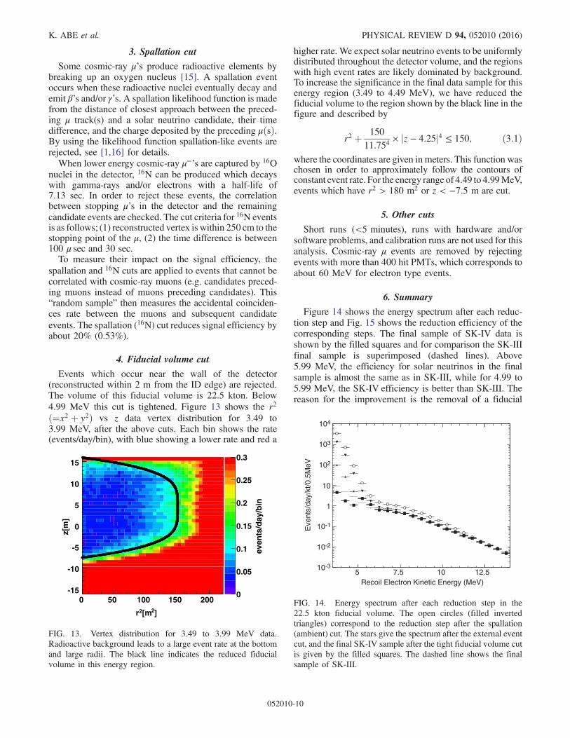
4. Fiducial volume cut

Events which occur near the wall of the detector(reconstructed within 2 m from the ID edge) are rejected.The volume of this fiducial volume is 22.5 kton. Below4.99 MeV this cut is tightened. Figure 13 shows the r2

ð¼x2 þ y2Þ vs z data vertex distribution for 3.49 to3.99 MeV, after the above cuts. Each bin shows the rate(events/day/bin), with blue showing a lower rate and red a

higher rate. We expect solar neutrino events to be uniformlydistributed throughout the detector volume, and the regionswith high event rates are likely dominated by background.To increase the significance in the final data sample for thisenergy region (3.49 to 4.49 MeV), we have reduced thefiducial volume to the region shown by the black line in thefigure and described by

r2 þ 150

11.754× jz − 4.25j4 ≤ 150; ð3:1Þ

where the coordinates are given in meters. This function waschosen in order to approximately follow the contours ofconstant event rate. For the energy range of 4.49 to 4.99MeV,events which have r2 > 180 m2 or z < −7.5 m are cut.

5. Other cuts

Short runs (<5 minutes), runs with hardware and/orsoftware problems, and calibration runs are not used for thisanalysis. Cosmic-ray μ events are removed by rejectingevents with more than 400 hit PMTs, which corresponds toabout 60 MeV for electron type events.

6. Summary

Figure 14 shows the energy spectrum after each reduc-tion step and Fig. 15 shows the reduction efficiency of thecorresponding steps. The final sample of SK-IV data isshown by the filled squares and for comparison the SK-IIIfinal sample is superimposed (dashed lines). Above5.99 MeV, the efficiency for solar neutrinos in the finalsample is almost the same as in SK-III, while for 4.99 to5.99 MeV, the SK-IV efficiency is better than SK-III. Thereason for the improvement is the removal of a fiducial

0

0.05

0.1

0.15

0.2

0.25

0.3

]2[m2r

0 50 100 150 200

z[m

]

-15

-10

-5

0

5

10

15

even

ts/d

ay/b

in

FIG. 13. Vertex distribution for 3.49 to 3.99 MeV data.Radioactive background leads to a large event rate at the bottomand large radii. The black line indicates the reduced fiducialvolume in this energy region.

10-3

10-2

10-1

1

10

102

103

104

5 7.5 10 12.5Recoil Electron Kinetic Energy (MeV)

Eve

nts/

day/

kt/0

.5M

eV

FIG. 14. Energy spectrum after each reduction step in the22.5 kton fiducial volume. The open circles (filled invertedtriangles) correspond to the reduction step after the spallation(ambient) cut. The stars give the spectrum after the external eventcut, and the final SK-IV sample after the tight fiducial volume cutis given by the filled squares. The dashed line shows the finalsample of SK-III.


052010-10

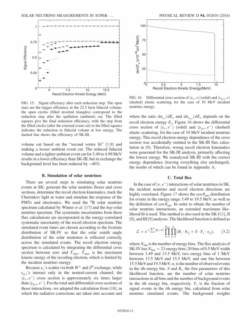
volume cut based on the “second vertex fit” [1,9] andmaking a looser ambient event cut. The reduced fiducialvolume and a tighter ambient event cut for 3.49 to 4.99MeVresults in a lower efficiency than SK-III, but in exchange thebackground level has been reduced by ∼40%.

B. Simulation of solar neutrinos

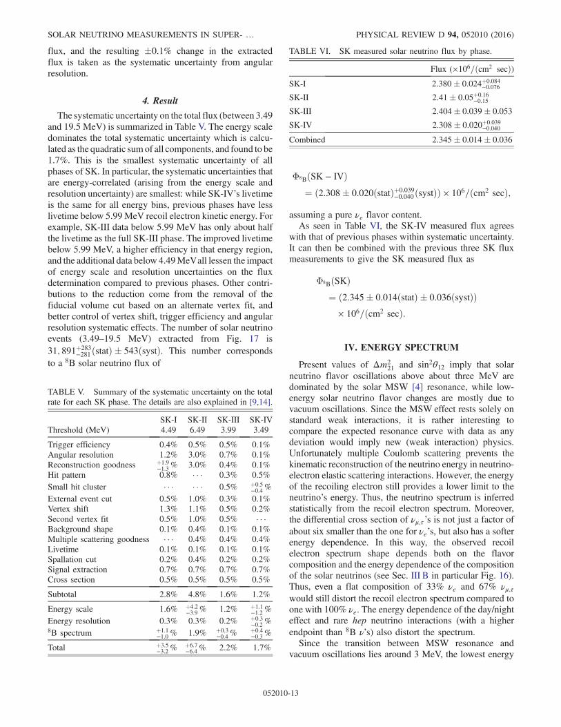
There are several steps in simulating solar neutrinoevents at SK: generate the solar neutrino fluxes and crosssections, determine the recoil electron kinematics, track theCherenkov light in water and simulate the response of thePMTs and electronics. We used the 8B solar neutrinospectrum calculated by Winter et al. [17] and the hep solarneutrino spectrum. The systematic uncertainties from theseflux calculations are incorporated in the energy-correlatedsystematic uncertainty of the recoil electron spectrum. Thesimulated event times are chosen according to the livetimedistribution of SK-IV so that the solar zenith angledistribution of the solar neutrinos is reflected correctlyacross the simulated events. The recoil electron energyspectrum is calculated by integrating the differential crosssection between zero and Tmax. Tmax is the maximumkinetic energy of the recoiling electron, which is limited bythe incident neutrino energy.Because νe’s scatter via bothW� and Z0 exchange, while

νμ;τ’s interact only in the neutral-current channel, theðνe; e−Þ cross section is approximately six times largerthan ðνμ;τ; e−Þ. For the total and differential cross sections ofthose interactions, we adopted the calculation from [18], inwhich the radiative corrections are taken into account and

where the ratio dσνe=dEe and dσνμ;τ=dEe depends on therecoil electron energy Ee. Figure 16 shows the differentialcross section of ðνe; e−Þ (solid) and ðνμ;τ; e−Þ (dashed)elastic scattering, for the case of 10 MeV incident neutrinoenergy. This recoil electron energy dependence of the crosssection was accidentally omitted in the SK-III flux calcu-lation in [9]. Therefore, wrong recoil electron kinematicswere generated for the SK-III analysis, primarily affectingthe lowest energy. We reanalyzed SK-III with the correctenergy dependence (leaving everything else unchanged),the results of which can be found in Appendix A.

C. Total flux

In the case of ðν; e−Þ interactions of solar neutrinos in SK,the incident neutrino and recoil electron directions arehighly correlated. Figure 17 shows the cos θsun distributionfor events in the energy range 3.49 to 19.5 MeV, as well asthe definition of cos θsun. In order to obtain the number ofsolar neutrino interactions, an extended maximum like-lihood fit is used. This method is also used in the SK-I [1], II[8], and III [9] analyses. The likelihood function is defined as

L ¼ e−ðP

iBiþSÞYNbin

i¼1

Ynij¼1

ðBi · bij þ S · Yi · sijÞ; ð3:2Þ

whereNbin is the number of energy bins. The flux analysis ofSK-IV hasNbin ¼ 23 energy bins; 20 bins of 0.5MeVwidthbetween 3.49 and 13.5 MeV, two energy bins of 1 MeVbetween 13.5 MeV and 15.5 MeV, and one bin between15.5MeVand19.5MeV.ni is the number of observed eventsin the ith energy bin. S and Bi, the free parameters of thislikelihood function, are the number of solar neutrinointeractions in all bins and the number of background eventsin the ith energy bin, respectively. Yi is the fraction ofsignal events in the ith energy bin, calculated from solarneutrino simulated events. The background weights

0

0.25

0.5

0.75

1

5 7.5 10 12.5 Recoil Electron Kinetic Energy (MeV)

Sig

nal E

ffici

ency

FIG. 15. Signal efficiency after each reduction step. The openstars are the trigger efficiency in the 22.5 kton fiducial volume,the open circles (filled inverted triangles) correspond to thereduction step after the spallation (ambient) cut. The filledsquares give the final reduction efficiency, with the step fromthe filled circles (after the external event cut) to the filled squaresindicates the reduction in fiducial volume at low energy. Thedashed line shows the efficiency of SK-III.

0

25

50

75

100

0 2.5 5 7.5 10Recoil Electron Kinetic Energy(MeV)

d σ/d

Te

(x10

-46 cm

2 /MeV

)

FIG. 16. Differential cross section of ðνe; eÞ (solid) and ðνμ;τ; eÞ(dashed) elastic scattering for the case of 10 MeV incidentneutrino energy.


052010-11

bij ¼ βiðcos θsunij Þ and the signal weights sij ¼ σðcos θsunij ;EijÞ are calculated from the expected shapes of the back-ground and solar neutrino signal, respectively (probabilitydensity functions). The background shapes βi are based onthe zenith and azimuthal angular distributions of real data,while the signal shapes σ are obtained from the solarneutrino simulated events. The values of S and Bi areobtained by maximizing the likelihood. The histogram ofFig. 17 is the best fit to the data, the dark (light) shadedregion is the solar neutrino signal (background) componentof that best fit. The systematic uncertainty for this method ofsignal extraction is estimated to be 0.7%.

1. Vertex shift systematic uncertainty

The systematic uncertainty resulting from the fiducialvolume cut comes from event vertex shifts. To calculate theeffect on the elastic scattering rate, the reconstructed vertexpositions of solar neutrino MC events are artificially shiftedfollowing the arrows in Fig. 3, and the number of eventspassing the fiducial volume cut with and without theartificial shift are compared. Figure 18 shows the energydependence of the systematic uncertainty coming from theshifting of the vertices. The increase below 4.99 MeVcomes from the reduced fiducial volume (smaller surface tovolume ratio), not from an energy dependence of the vertexshift. The systematic uncertainty on the total rate is�0.2%.

2. Trigger efficiency systematic uncertainty

The trigger efficiency depends on the vertex position,water transparency, number of hit PMTs, and response ofthe front-end electronics. The systematic uncertainty

from the trigger efficiency is estimated by comparingNi-calibration data (see Sec. II C) with MC simula-tion. For 3.49–3.99 MeV and 3.99–4.49 MeV, the differ-ence between data and MC is −3.43� 0.37% and−0.86� 0.31%, respectively [14]. Above 4.49 MeV thetrigger efficiency is 100% and its uncertainty is negligible.The resulting total flux systematic uncertainty due to thetrigger efficiency is �0.1%.

3. Angular resolution systematic uncertainty

The angular resolution of electrons is defined as theangle which includes 68% of events in the distribution ofthe angular difference between their reconstructed directionand their true direction. The MC prediction of the angularresolution is checked and the systematic uncertainty isestimated by comparing the difference in the reconstructedand true directions of LINAC data and LINAC (see [12])simulated events. This difference is shown in Table IV forvarious energies. To estimate the systematic uncertainty onthe total flux, the signal shapes sangþij and sang−ij are varied byshifting the reconstructed directions of the simulated solarneutrino events by the uncertainty in the angular resolution.These new signal shapes are used when extracting the total

Recoil electon kinetic energy [MeV]4 6 8 10 12 14 16 18V

erte

x sh

ift

syst

emat

ic u

nce

rtai

nty

[%

]

0

0.1

0.2

0.3

0.4

0.5

FIG. 18. Vertex shift systematic uncertainty on the flux. Theincrease below 4.99 MeV comes from the tight fiducial volumecut. (see text).

TABLE IV. Angular resolution difference between LINAC dataand simulated LINAC events for each SK phase. The energyrefers to the electron’s in-tank kinetic energy.

Energy (MeV) SK-I(%) SK-II(%) SK-III(%) SK-IV(%)

4.0 � � � � � � � � � 0.644.4 −1.64 � � � 0.74 0.685.3 −1.38 � � � � � � � � �6.3 2.32 5.93 � � � 0.028.2 2.33 7.10 0.40 0.0610.3 1.52 � � � � � � � � �12.9 1.07 6.50 −0.27 0.2215.6 0.88 � � � 0.39 � � �18.2 � � � � � � � � � 0.31

z

Sun

rν

rrec θzθsun

0

0.1

0.2

0.3

-1 -0.5 0 0.5 1

cosθsun

Eve

nts/

day/

kton

/bin

FIG. 17. Solar angle distribution for 3.49 to 19.5 MeV. θsun isthe angle between the incoming neutrino direction rν and thereconstructed recoil electron direction rrec. θz is the solar zenithangle. Black points are data while the histogram is the best fit tothe data. The dark (light) shaded region is the solar neutrinosignal (background) component of this fit.


052010-12

flux, and the resulting �0.1% change in the extractedflux is taken as the systematic uncertainty from angularresolution.

4. Result

The systematic uncertainty on the total flux (between 3.49and 19.5 MeV) is summarized in Table V. The energy scaledominates the total systematic uncertainty which is calcu-lated as the quadratic sumof all components, and found to be1.7%. This is the smallest systematic uncertainty of allphases of SK. In particular, the systematic uncertainties thatare energy-correlated (arising from the energy scale andresolution uncertainty) are smallest: while SK-IV’s livetimeis the same for all energy bins, previous phases have lesslivetime below 5.99 MeV recoil electron kinetic energy. Forexample, SK-III data below 5.99 MeV has only about halfthe livetime as the full SK-III phase. The improved livetimebelow 5.99 MeV, a higher efficiency in that energy region,and the additional data below 4.49MeVall lessen the impactof energy scale and resolution uncertainties on the fluxdetermination compared to previous phases. Other contri-butions to the reduction come from the removal of thefiducial volume cut based on an alternate vertex fit, andbetter control of vertex shift, trigger efficiency and angularresolution systematic effects. The number of solar neutrinoevents (3.49–19.5 MeV) extracted from Fig. 17 is31; 891þ283

−281ðstatÞ � 543ðsystÞ. This number correspondsto a 8B solar neutrino flux of

Φ8BðSK − IVÞ¼ ð2.308� 0.020ðstatÞþ0.039

−0.040ðsystÞÞ × 106=ðcm2 secÞ;

assuming a pure νe flavor content.As seen in Table VI, the SK-IV measured flux agrees

with that of previous phases within systematic uncertainty.It can then be combined with the previous three SK fluxmeasurements to give the SK measured flux as

Φ8BðSKÞ¼ ð2.345� 0.014ðstatÞ � 0.036ðsystÞÞ× 106=ðcm2 secÞ:

IV. ENERGY SPECTRUM

Present values of Δm221 and sin2θ12 imply that solar

neutrino flavor oscillations above about three MeV aredominated by the solar MSW [4] resonance, while low-energy solar neutrino flavor changes are mostly due tovacuum oscillations. Since the MSW effect rests solely onstandard weak interactions, it is rather interesting tocompare the expected resonance curve with data as anydeviation would imply new (weak interaction) physics.Unfortunately multiple Coulomb scattering prevents thekinematic reconstruction of the neutrino energy in neutrino-electron elastic scattering interactions. However, the energyof the recoiling electron still provides a lower limit to theneutrino’s energy. Thus, the neutrino spectrum is inferredstatistically from the recoil electron spectrum. Moreover,the differential cross section of νμ;τ ’s is not just a factor ofabout six smaller than the one for νe’s, but also has a softerenergy dependence. In this way, the observed recoilelectron spectrum shape depends both on the flavorcomposition and the energy dependence of the compositionof the solar neutrinos (see Sec. III B in particular Fig. 16).Thus, even a flat composition of 33% νe and 67% νμ;τwould still distort the recoil electron spectrum compared toone with 100% νe. The energy dependence of the day/nighteffect and rare hep neutrino interactions (with a higherendpoint than 8B ν’s) also distort the spectrum.Since the transition between MSW resonance and

vacuum oscillations lies around 3 MeV, the lowest energy

TABLE V. Summary of the systematic uncertainty on the totalrate for each SK phase. The details are also explained in [9,14].

SK-I SK-II SK-III SK-IVThreshold (MeV) 4.49 6.49 3.99 3.49

Trigger efficiency 0.4% 0.5% 0.5% 0.1%Angular resolution 1.2% 3.0% 0.7% 0.1%Reconstruction goodness þ1.9

−1.3 % 3.0% 0.4% 0.1%Hit pattern 0.8% � � � 0.3% 0.5%Small hit cluster � � � � � � 0.5% þ0.5

−0.4 %

External event cut 0.5% 1.0% 0.3% 0.1%Vertex shift 1.3% 1.1% 0.5% 0.2%Second vertex fit 0.5% 1.0% 0.5% � � �Background shape 0.1% 0.4% 0.1% 0.1%Multiple scattering goodness � � � 0.4% 0.4% 0.4%Livetime 0.1% 0.1% 0.1% 0.1%Spallation cut 0.2% 0.4% 0.2% 0.2%Signal extraction 0.7% 0.7% 0.7% 0.7%Cross section 0.5% 0.5% 0.5% 0.5%

Subtotal 2.8% 4.8% 1.6% 1.2%

Energy scale 1.6% þ4.2−3.9 % 1.2% þ1.1

−1.2 %

Energy resolution 0.3% 0.3% 0.2% þ0.3−0.2 %

8B spectrum þ1.1−1.0 % 1.9% þ0.3

−0.4 %þ0.4−0.3 %

Total þ3.5−3.2 %

þ6.7−6.4 % 2.2% 1.7%

TABLE VI. SK measured solar neutrino flux by phase.

Flux (×106=ðcm2 secÞ)SK-I 2.380� 0.024þ0.084

−0.076

SK-II 2.41� 0.05þ0.16−0.15

SK-III 2.404� 0.039� 0.053

SK-IV 2.308� 0.020þ0.039−0.040

Combined 2.345� 0.014� 0.036


052010-13

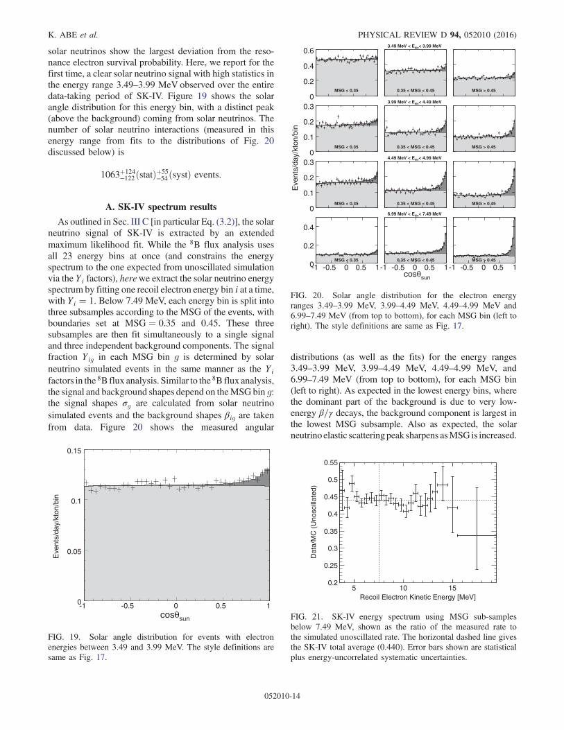
solar neutrinos show the largest deviation from the reso-nance electron survival probability. Here, we report for thefirst time, a clear solar neutrino signal with high statistics inthe energy range 3.49–3.99 MeV observed over the entiredata-taking period of SK-IV. Figure 19 shows the solarangle distribution for this energy bin, with a distinct peak(above the background) coming from solar neutrinos. Thenumber of solar neutrino interactions (measured in thisenergy range from fits to the distributions of Fig. 20discussed below) is

1063þ124−122ðstatÞþ55

−54ðsystÞ events:

A. SK-IV spectrum results

As outlined in Sec. III C [in particular Eq. (3.2)], the solarneutrino signal of SK-IV is extracted by an extendedmaximum likelihood fit. While the 8B flux analysis usesall 23 energy bins at once (and constrains the energyspectrum to the one expected from unoscillated simulationvia the Yi factors), herewe extract the solar neutrino energyspectrum by fitting one recoil electron energy bin i at a time,with Yi ¼ 1. Below 7.49 MeV, each energy bin is split intothree subsamples according to the MSG of the events, withboundaries set at MSG ¼ 0.35 and 0.45. These threesubsamples are then fit simultaneously to a single signaland three independent background components. The signalfraction Yig in each MSG bin g is determined by solarneutrino simulated events in the same manner as the Yi

factors in the 8B flux analysis. Similar to the 8B flux analysis,the signal and background shapes depend on theMSG bin g:the signal shapes σg are calculated from solar neutrinosimulated events and the background shapes βig are takenfrom data. Figure 20 shows the measured angular

distributions (as well as the fits) for the energy ranges3.49–3.99 MeV, 3.99–4.49 MeV, 4.49–4.99 MeV, and6.99–7.49 MeV (from top to bottom), for each MSG bin(left to right). As expected in the lowest energy bins, wherethe dominant part of the background is due to very low-energy β=γ decays, the background component is largest inthe lowest MSG subsample. Also as expected, the solarneutrino elastic scatteringpeak sharpens asMSG is increased.

0

0.05

0.1

0.15

-1 -0.5 0 0.5 1cosθsun

Eve

nts/

day/

kton

/bin

FIG. 19. Solar angle distribution for events with electronenergies between 3.49 and 3.99 MeV. The style definitions aresame as Fig. 17.

0

0.2

0.4

0.6

MSG < 0.35

3.49 MeV < Ekin< 3.99 MeV




0.35 < MSG < 0.45 MSG > 0.45

0

0.1

0.2

0.3

Eve

nts/

day/

kton

/bin

MSG < 0.35 0.35 < MSG < 0.45 MSG > 0.45

0

0.1

0.2

0.3

MSG < 0.35 0.35 < MSG < 0.45 MSG > 0.45

0

0.2

0.4

MSG < 0.35

cosθsun

0.35 < MSG < 0.45

-1 -0.5 0 0.5 1-1 -0.5 0 0.5 1-1 -0.5 0 0.5 1MSG > 0.45

FIG. 20. Solar angle distribution for the electron energyranges 3.49–3.99 MeV, 3.99–4.49 MeV, 4.49–4.99 MeV and6.99–7.49 MeV (from top to bottom), for each MSG bin (left toright). The style definitions are same as Fig. 17.

Recoil Electron Kinetic Energy [MeV]5 10 15

Dat

a/M

C (

Uno

scill

ated

)

0.2

0.25

0.3

0.35

0.4

0.45

0.5

0.55

FIG. 21. SK-IV energy spectrum using MSG sub-samplesbelow 7.49 MeV, shown as the ratio of the measured rate tothe simulated unoscillated rate. The horizontal dashed line givesthe SK-IV total average (0.440). Error bars shown are statisticalplus energy-uncorrelated systematic uncertainties.


052010-14

Using this method for recoil electron energy bins below7.49 MeV gives ∼10% improvement in the statisticaluncertainty on the number of extracted signal events (theadditional systematic uncertainty is small compared to thestatistical gain). Figure 21 shows the resulting SK-IVenergy spectrum, where below 7.49 MeV MSG has beenused and above 7.49 MeV the standard signal extractionmethod without MSG is used. Table XVI in Appendix Bgives the measured and expected rate in each energy bin,as well as that measured for the day and night timesseparately, along with the 1σ statistical deviations. Wereanalyzed the SK-III spectrum below 7.49 MeV with thesame method, the same MSG bins and the same energybins as SK-IV, down to 3.99 MeV. We also refit the entireSK-II (which has poorer resolution) spectrum using thesame three MSG sub-samples. The gains in precision aresimilar to SK-IV. The SK-II and III spectra are given inSec. IV C.To analyze the spectrum, we simultaneously fit the SK-I,

II, III and IV spectra to their predictions, while varying the

8B and hep neutrino fluxes within uncertainties. The 8Bflux is constrained to ð5.25� 0.20Þ × 106=ðcm2 secÞ andthe hep flux to ð8� 16Þ × 103=ðcm2 secÞ (motivated bySNO’s measurement [19] and limit [20]). The χ2 isdescribed in detail in Sec. VI.

B. Systematic uncertainties on the energy spectrum

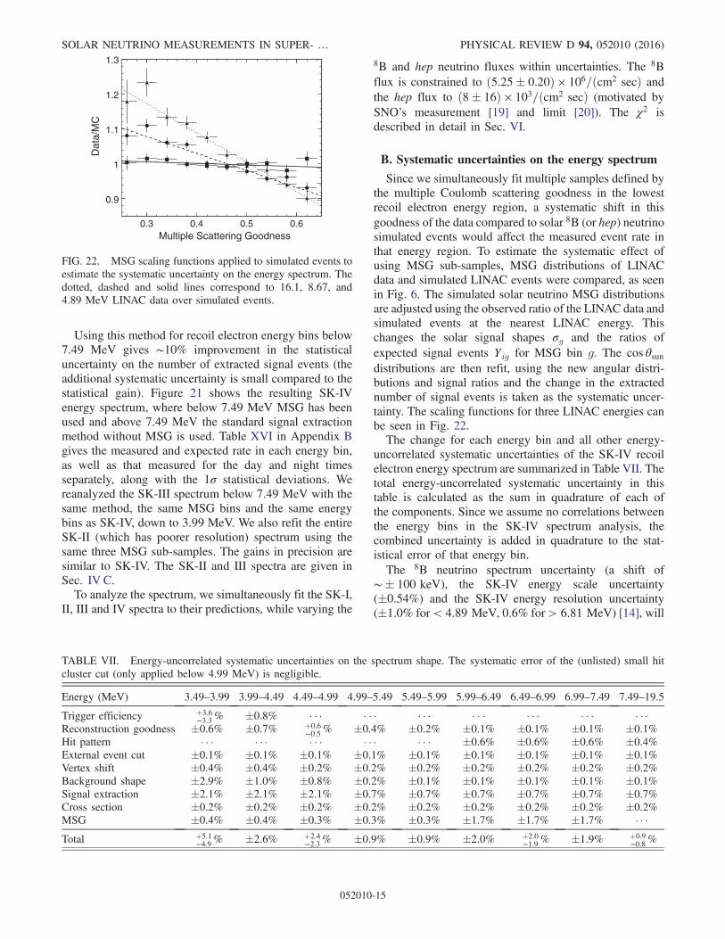
Since we simultaneously fit multiple samples defined bythe multiple Coulomb scattering goodness in the lowestrecoil electron energy region, a systematic shift in thisgoodness of the data compared to solar 8B (or hep) neutrinosimulated events would affect the measured event rate inthat energy region. To estimate the systematic effect ofusing MSG sub-samples, MSG distributions of LINACdata and simulated LINAC events were compared, as seenin Fig. 6. The simulated solar neutrino MSG distributionsare adjusted using the observed ratio of the LINAC data andsimulated events at the nearest LINAC energy. Thischanges the solar signal shapes σg and the ratios ofexpected signal events Yig for MSG bin g. The cos θsundistributions are then refit, using the new angular distri-butions and signal ratios and the change in the extractednumber of signal events is taken as the systematic uncer-tainty. The scaling functions for three LINAC energies canbe seen in Fig. 22.The change for each energy bin and all other energy-

uncorrelated systematic uncertainties of the SK-IV recoilelectron energy spectrum are summarized in Table VII. Thetotal energy-uncorrelated systematic uncertainty in thistable is calculated as the sum in quadrature of each ofthe components. Since we assume no correlations betweenthe energy bins in the SK-IV spectrum analysis, thecombined uncertainty is added in quadrature to the stat-istical error of that energy bin.The 8B neutrino spectrum uncertainty (a shift of

∼� 100 keV), the SK-IV energy scale uncertainty(�0.54%) and the SK-IV energy resolution uncertainty(�1.0% for< 4.89 MeV, 0.6% for > 6.81 MeV) [14], will

Multiple Scattering Goodness

Dat

a/M

C

0.9

1

1.1

1.2

1.3

0.3 0.4 0.5 0.6

FIG. 22. MSG scaling functions applied to simulated events toestimate the systematic uncertainty on the energy spectrum. Thedotted, dashed and solid lines correspond to 16.1, 8.67, and4.89 MeV LINAC data over simulated events.

TABLE VII. Energy-uncorrelated systematic uncertainties on the spectrum shape. The systematic error of the (unlisted) small hitcluster cut (only applied below 4.99 MeV) is negligible.

Energy (MeV) 3.49–3.99 3.99–4.49 4.49–4.99 4.99–5.49 5.49–5.99 5.99–6.49 6.49–6.99 6.99–7.49 7.49–19.5Trigger efficiency þ3.6

−3.3 % �0.8% � � � � � � � � � � � � � � � � � � � � �Reconstruction goodness �0.6% �0.7% þ0.6

−0.5 % �0.4% �0.2% �0.1% �0.1% �0.1% �0.1%Hit pattern � � � � � � � � � � � � � � � �0.6% �0.6% �0.6% �0.4%External event cut �0.1% �0.1% �0.1% �0.1% �0.1% �0.1% �0.1% �0.1% �0.1%Vertex shift �0.4% �0.4% �0.2% �0.2% �0.2% �0.2% �0.2% �0.2% �0.2%Background shape �2.9% �1.0% �0.8% �0.2% �0.1% �0.1% �0.1% �0.1% �0.1%Signal extraction �2.1% �2.1% �2.1% �0.7% �0.7% �0.7% �0.7% �0.7% �0.7%Cross section �0.2% �0.2% �0.2% �0.2% �0.2% �0.2% �0.2% �0.2% �0.2%MSG �0.4% �0.4% �0.3% �0.3% �0.3% �1.7% �1.7% �1.7% � � �Total þ5.1

−4.9 % �2.6% þ2.4−2.3 % �0.9% �0.9% �2.0% þ2.0

−1.9 % �1.9% þ0.9−0.8 %


052010-15

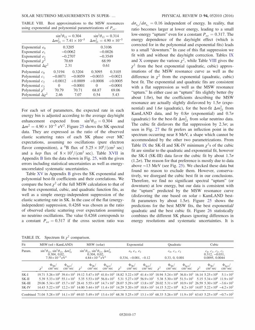
shift all energy bins in a correlated manner. The size andcorrelation of these uncertainties are calculated from theneutrino spectrum, the differential cross section, the energyresolution function, and the size of the systematic shifts. Wevary each of these three parameters (8B neutrino spectrumshift, energy scale, and energy resolution) individually.Figure 23 shows the result of this calculation. When weanalyze the spectrum, we apply these shifts to the spectralpredictions. When the SK-IV spectrum is combined withthe SK-I, II, and III spectra, the 8B neutrino spectrum shiftis common to all four phases, while each phase varies itsenergy scale and resolution individually (without correla-tion between the phases).

C. SK-I/II/III/IV combined spectrum analysis

In order to discuss the energy dependence of thesolar neutrino flavor composition in a general way,SNO [19] has parametrized the electron survival prob-ability Pee using a quadratic function centered at10 MeV:

PeeðEνÞ ¼ c0 þ c1

�Eν

MeV− 10

�þ c2

�Eν

MeV− 10

�2

;

ð4:1Þ

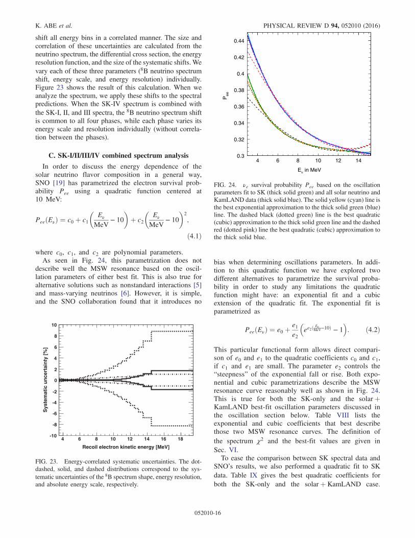
where c0, c1, and c2 are polynomial parameters.As seen in Fig. 24, this parametrization does not

describe well the MSW resonance based on the oscil-lation parameters of either best fit. This is also true foralternative solutions such as nonstandard interactions [5]and mass-varying neutrinos [6]. However, it is simple,and the SNO collaboration found that it introduces no

bias when determining oscillations parameters. In addi-tion to this quadratic function we have explored twodifferent alternatives to parametrize the survival proba-bility in order to study any limitations the quadraticfunction might have: an exponential fit and a cubicextension of the quadratic fit. The exponential fit isparametrized as

PeeðEνÞ ¼ e0 þe1e2

�ee2ð

EνMeV−10Þ − 1

�: ð4:2Þ

This particular functional form allows direct compari-son of e0 and e1 to the quadratic coefficients c0 and c1,if c1 and e1 are small. The parameter e2 controls the“steepness” of the exponential fall or rise. Both expo-nential and cubic parametrizations describe the MSWresonance curve reasonably well as shown in Fig. 24.This is true for both the SK-only and the solar þKamLAND best-fit oscillation parameters discussed inthe oscillation section below. Table VIII lists theexponential and cubic coefficients that best describethose two MSW resonance curves. The definition ofthe spectrum χ2 and the best-fit values are given inSec. VI.To ease the comparison between SK spectral data and

SNO’s results, we also performed a quadratic fit to SKdata. Table IX gives the best quadratic coefficients forboth the SK-only and the solar þ KamLAND case.

Recoil electron kinetic energy [MeV]

4 6 8 10 12 14 16 18

Sys

tem

atic

un

cert

ain

ty [

%]

-10

-8

-6

-4

-2

0

2

4

6

8

10

FIG. 23. Energy-correlated systematic uncertainties. The dot-dashed, solid, and dashed distributions correspond to the sys-tematic uncertainties of the 8B spectrum shape, energy resolution,and absolute energy scale, respectively.

Eν in MeV

Pee

0.3

0.32

0.34

0.36

0.38

0.4

0.42

0.44

4 6 8 10 12 14

FIG. 24. νe survival probability Pee based on the oscillationparameters fit to SK (thick solid green) and all solar neutrino andKamLAND data (thick solid blue). The solid yellow (cyan) line isthe best exponential approximation to the thick solid green (blue)line. The dashed black (dotted green) line is the best quadratic(cubic) approximation to the thick solid green line and the dashedred (dotted pink) line the best quadratic (cubic) approximation tothe thick solid blue.


052010-16

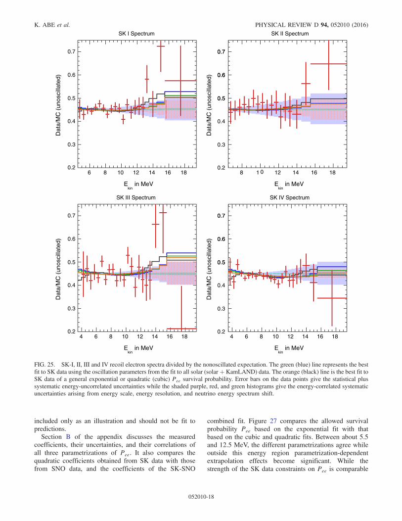
For each set of parameters, the expected rate in eachenergy bin is adjusted according to the average day/nightenhancement expected from sin2θ12 ¼ 0.304 andΔm2 ¼ 4.90 × 10−5 eV2. Figure 25 shows the SK spectraldata. They are expressed as the ratio of the observedelastic scattering rates of each SK phase over MCexpectations, assuming no oscillations (pure electronflavor composition), a 8B flux of 5.25 × 106=ðcm2 secÞand a hep flux of 8 × 103=ðcm2 secÞ. Table XVII inAppendix B lists the data shown in Fig. 25, with the givenerrors including statistical uncertainties as well as energy-uncorrelated systematic uncertainties.Table XV in Appendix B gives the SK exponential and

polynomial best-fit coefficients and their correlations. Wecompare the best χ2 of the full MSW calculation to that ofthe best exponential, cubic, and quadratic function fits, aswell as a simple energy-independent suppression of theelastic scattering rate in SK. In the case of the flat (energy-independent) suppression, 0.4268 was chosen as the ratioof observed elastic scattering over expectation assumingno neutrino oscillations. The value 0.4268 corresponds toa constant Pee ¼ 0.317 if the cross section ratio was

dσνμ=dσνe ¼ 0.16 independent of energy. In reality, thatratio becomes larger at lower energy, leading to a smalllow-energy “upturn” even for a constant Pee ¼ 0.317. Theenergy dependence of the day/night effect (which iscorrected for in the polynomial and exponential fits) leadsto a small “downturn.” In case of this flat suppression wefit with and without the day/night correction. Tables IXand X compare the various χ2, while Table VIII gives theχ2 from the best exponential (quadratic, cubic) approx-imations of the MSW resonance curve as well as thedifference in χ2 from the exponential (quadratic, cubic)best fit. The exponential and quadratic fits are consistentwith a flat suppression as well as the MSW resonance“upturn.” In either case an “upturn” fits slightly better (byabout 1.0σ), but the coefficients describing the MSWresonance are actually slightly disfavored by 1.5σ (expo-nential) and 1.6σ (quadratic), for the best-fit Δm2

21 fromKamLAND data, and by 0.8σ (exponential) and 0.7σ(quadratic) for the best-fit Δm2

21 from solar neutrino data.The cubic fit disfavors the flat suppression by 2.3σ; asseen in Fig. 27 the fit prefers an inflection point in thespectrum occurring near 8 MeV, a shape which cannot beaccommodated by the other two parametrizations. FromTable IX the SK-II and SK-IV minimum χ2s of the cubicfit are similar to the quadratic and exponential fit, howeverthe SK-I (SK-III) data favor the cubic fit by about 1.7σ(1.2σ). The reason for that preference is mostly due to dataabove ∼13 MeV (see Fig. 25). We checked these data butfound no reason to exclude them. However, conserva-tively, we disregard the cubic best fit in our conclusions.Therefore, we find no significant spectral “upturn” (ordownturn) at low energy, but our data is consistent withthe “upturn” predicted by the MSW resonance curve(disfavoring the one based on solar þ KamLAND best-fit parameters by about 1.5σ). Figure 25 shows thepredictions for the best MSW fits, the best exponential/quadratic and the best cubic fit. Figure 26 statisticallycombines the different SK phases ignoring differences inenergy resolutions and systematic uncertainties. It is

TABLE IX. Spectrum fit χ2 comparison.

Fit MSW (solþKamLAND) MSW (solar) Exponential Quadratic Cubic

Param. sin2θ12, sin2θ13, Δm221 sin2θ12, sin2θ13, Δm2

21 e0 e1, e2 c0, c1, c2 c0, c1, c2, c30.304, 0.02,

7.50×10−5 eV20.304, 0.02,

4.84×10−5 eV2 0.334, −0.001, −0.12 0.33, 0, 0.0010.312, −0.031,0.0095, 0.0044

χ2Φ8B=cm2 sec

Φhep=cm2 sec χ2

Φ8B=cm2 sec

Φhep=cm2 sec χ2

Φ8B=cm2 sec

Φhep=cm2 sec χ2

Φ8B=cm2 sec

Φhep=cm2 sec χ2

Φ8B=cm2 sec

Φhep=cm2 sec

SK-I 19.71 5.26×106 39.4×103 19.12 5.47×106 41.0×103 18.82 5.22×106 41.4×103 18.94 5.24×106 36.8×103 16.14 5.25×106 5.1×103

SK-II 5.39 5.33×106 55.1×103 5.35 5.53×106 56.8×103 5.31 5.27×106 56.9×103 5.38 5.30×106 51.5×103 5.15 5.34×106 11.9×103

SK-III 29.06 5.34×106 15.7×103 28.41 5.55×106 14.7×103 28.07 5.29×106 13.8×103 28.02 5.31×106 10.9×103 26.59 5.30×106 −3.6×103

SK-IV 14.43 5.22×106 12.2×103 14.00 5.44×106 11.4×103 14.29 5.20×106 10.8×103 14.15 5.22×106 8.2×103 14.07 5.22×106 −4.2×103

Combined 71.04 5.28×106 14.1×103 69.03 5.49×106 13.4×103 68.38 5.25×106 13.1×103 68.33 5.26×106 11.9×103 63.63 5.25×106 −0.7×103

TABLE VIII. Best approximations to the MSW resonancesusing exponential and polynomial parametrizations of Pee.

sin2θ12 ¼ 0.304 sin2θ12 ¼ 0.314Δm2

21 ¼ 7.41 × 10−5 Δm221 ¼ 4.90 × 10−5

Exponential e0 0.3205 0.3106Exponential e1 −0.0062 −0.0026Exponential e2 −0.2707 −0.3549Exponential χ2 70.69 68.99Exponential Δχ2 2.31 0.61

Polynomial c0 0.3194 0.3204 0.3095 0.3105Polynomial c1 −0.0071 −0.0059 −0.0033 −0.0021Polynomial c2 þ0.0012 þ0.0009 þ0.0008 þ0.0005Polynomial c3 0 −0.0001 0 −0.0001Polynomial χ2 70.79 70.71 68.87 69.06Polynomial Δχ2 2.46 7.07 0.54 5.43


052010-17

included only as an illustration and should not be fit topredictions.Section B of the appendix discusses the measured

coefficients, their uncertainties, and their correlations ofall three parametrizations of Pee. It also compares thequadratic coefficients obtained from SK data with thosefrom SNO data, and the coefficients of the SK-SNO

combined fit. Figure 27 compares the allowed survivalprobability Pee based on the exponential fit with thatbased on the cubic and quadratic fits. Between about 5.5and 12.5 MeV, the different parametrizations agree whileoutside this energy region parametrization-dependentextrapolation effects become significant. While thestrength of the SK data constraints on Pee is comparable

in MeVkin

E

0.2

0.3

0.4

0.5

0.6

0.7D

ata/

MC

(un

osci

llate

d)

SK I Spectrum

in MeVkin

E

0.2

0.3

0.4

0.50.5

0.60.6

0.70.7

Dat

a/M

C (

unos

cilla

ted)

SK II Spectrum

in MeVkin

E

0.2

0.3

0.4

0.5

0.6

0.7

Dat

a/M

C (

unos

cilla

ted)

SK III Spectrum

in MeVkin

E

6 8 10 12 14 16 18 8 1 12 14 16 18

4 6 8 10 12 14 16 18 4 6 8 10 12 14 16 180.2

0.3

0.4

0.50.5

0.60.6

0.70.7D

ata/

MC

(un

osci

llate

d)

SK IV Spectrum

0

FIG. 25. SK-I, II, III and IV recoil electron spectra divided by the nonoscillated expectation. The green (blue) line represents the bestfit to SK data using the oscillation parameters from the fit to all solar (solar þ KamLAND) data. The orange (black) line is the best fit toSK data of a general exponential or quadratic (cubic) Pee survival probability. Error bars on the data points give the statistical plussystematic energy-uncorrelated uncertainties while the shaded purple, red, and green histograms give the energy-correlated systematicuncertainties arising from energy scale, energy resolution, and neutrino energy spectrum shift.


052010-18

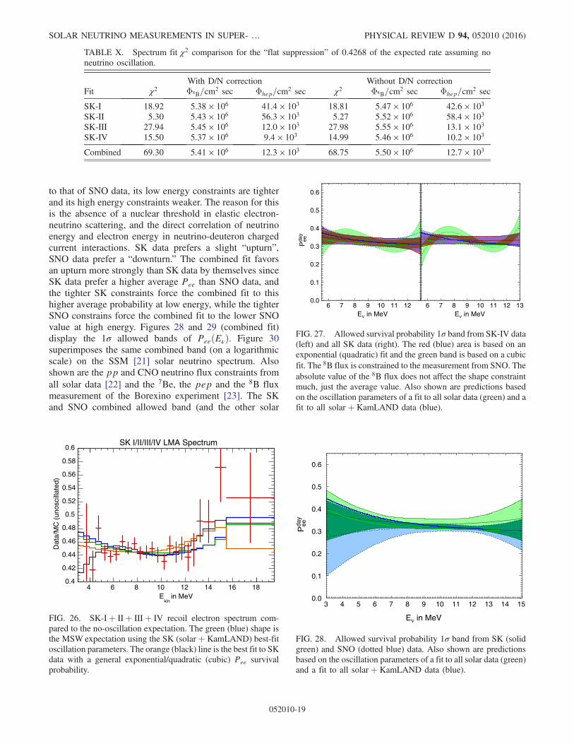
to that of SNO data, its low energy constraints are tighterand its high energy constraints weaker. The reason for thisis the absence of a nuclear threshold in elastic electron-neutrino scattering, and the direct correlation of neutrinoenergy and electron energy in neutrino-deuteron chargedcurrent interactions. SK data prefers a slight “upturn”,SNO data prefer a “downturn.” The combined fit favorsan upturn more strongly than SK data by themselves sinceSK data prefer a higher average Pee than SNO data, andthe tighter SK constraints force the combined fit to thishigher average probability at low energy, while the tighterSNO constrains force the combined fit to the lower SNOvalue at high energy. Figures 28 and 29 (combined fit)display the 1σ allowed bands of PeeðEνÞ. Figure 30superimposes the same combined band (on a logarithmicscale) on the SSM [21] solar neutrino spectrum. Alsoshown are the pp and CNO neutrino flux constraints fromall solar data [22] and the 7Be, the pep and the 8B fluxmeasurement of the Borexino experiment [23]. The SKand SNO combined allowed band (and the other solar

TABLE X. Spectrum fit χ2 comparison for the “flat suppression” of 0.4268 of the expected rate assuming noneutrino oscillation.

With D/N correction Without D/N correctionFit χ2 Φ8B=cm

2 sec Φhep=cm2 sec χ2 Φ8B=cm2 sec Φhep=cm2 sec

SK-I 18.92 5.38 × 106 41.4 × 103 18.81 5.47 × 106 42.6 × 103

SK-II 5.30 5.43 × 106 56.3 × 103 5.27 5.52 × 106 58.4 × 103

SK-III 27.94 5.45 × 106 12.0 × 103 27.98 5.55 × 106 13.1 × 103

SK-IV 15.50 5.37 × 106 9.4 × 103 14.99 5.46 × 106 10.2 × 103

Combined 69.30 5.41 × 106 12.3 × 103 68.75 5.50 × 106 12.7 × 103

in MeVkin

E4 6 8 10 12 14 16 18

Dat

a/M

C (

unos

cilla

ted)

0.4

0.42

0.44

0.46

0.48

0.5

0.52

0.54

0.56

0.58

0.6SK I/II/III/IV LMA Spectrum

FIG. 26. SK-Iþ IIþ IIIþ IV recoil electron spectrum com-pared to the no-oscillation expectation. The green (blue) shape isthe MSW expectation using the SK (solar þ KamLAND) best-fitoscillation parameters. The orange (black) line is the best fit to SKdata with a general exponential/quadratic (cubic) Pee survivalprobability.

Pee

0.0

0.1

0.2

0.3

0.4

0.5

0.6

Eν in MeV6 7 8 9 10 11 12

Eν in MeV6 7 8 9 10 11 12 13

day

FIG. 27. Allowed survival probability 1σ band from SK-IV data(left) and all SK data (right). The red (blue) area is based on anexponential (quadratic) fit and the green band is based on a cubicfit. The 8B flux is constrained to the measurement from SNO. Theabsolute value of the 8B flux does not affect the shape constraintmuch, just the average value. Also shown are predictions basedon the oscillation parameters of a fit to all solar data (green) and afit to all solar þ KamLAND data (blue).

0.0

0.1

0.2

0.3

0.4

0.5

0.6

Eν in MeV

3 4 5 6 7 8 9 10 11 12 13 14 15

Peeda

y

FIG. 28. Allowed survival probability 1σ band from SK (solidgreen) and SNO (dotted blue) data. Also shown are predictionsbased on the oscillation parameters of a fit to all solar data (green)and a fit to all solar þ KamLAND data (blue).


052010-19

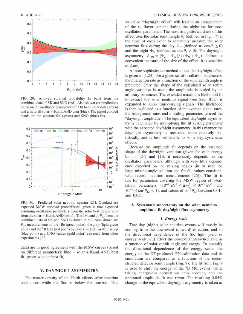
data) are in good agreement with the MSW curves (basedon different parameters: blue ¼ solar þ KamLAND bestfit, green ¼ solar best fit).

V. DAY/NIGHT ASYMMETRY

The matter density of the Earth affects solar neutrinooscillations while the Sun is below the horizon. This

so called “day/night effect” will lead to an enhancementof the νe flavor content during the nighttime for mostoscillation parameters. The most straightforward test of thiseffect uses the solar zenith angle θz (defined in Fig. 17) atthe time of each event to separately measure the solarneutrino flux during the day ΦD (defined as cos θz ≤ 0)and the night ΦN (defined as cos θz > 0). The day/nightasymmetry ADN ¼ ðΦD − ΦNÞ= 1

2ðΦD þ ΦN) defines a

convenient measure of the size of the effect; it is sensitiveto Δm2

21.A more sophisticated method to test the day/night effect

is given in [1,24]. For a given set of oscillation parameters,the interaction rate as a function of the solar zenith angle ispredicted. Only the shape of the calculated solar zenithangle variation is used; the amplitude is scaled by anarbitrary parameter. The extended maximum likelihood fitto extract the solar neutrino signal (see Sec. III C) isexpanded to allow time-varying signals. The likelihoodis then evaluated as a function of the average signal rates,the background rates and a scaling parameter, termed the“day/night amplitude”. The equivalent day/night asymme-try is calculated by multiplying the fit scaling parameterwith the expected day/night asymmetry. In this manner theday/night asymmetry is measured more precisely sta-tistically and is less vulnerable to some key systematiceffects.Because the amplitude fit depends on the assumed

shape of the day/night variation (given for each energybin in [24] and [1]), it necessarily depends on theoscillation parameters, although with very little depend-ence expected on the mixing angles (in or near thelarge mixing angle solution and for θ13 values consistentwith reactor neutrino measurements [25]). The fit isrun for parameters covering the MSW region of oscil-lation parameters (10−9 eV2 ≤ Δm2

21 ≤ 10−3 eV2 and10−4 ≤ sin2θ12 < 1), and values of sin2 θ13 between 0.015and 0.035.

A. Systematic uncertainty on the solar neutrinoamplitude fit day/night flux asymmetry

1. Energy scale

True day (night) solar neutrino events will mostly becoming from the downward (upward) direction, and sothe directional dependence of the SK light yield orenergy scale will affect the observed interaction rate asa function of solar zenith angle and energy. To quantifythe directional dependence of the energy scale, theenergy of the DT-produced 16N calibration data and itssimulation are compared as a function of the recon-structed detector zenith angle (Fig. 9). The fit from Fig. 9is used to shift the energy of the 8B MC events, whiletaking energy-bin correlations into account, and theunbinned amplitude fit was rerun. The resulting 0.05%change in the equivalent day/night asymmetry is taken as

Peeda

y

0.0

0.1

0.2

0.3

0.4

0.5

0.6

Eν in MeV

3 4 5 6 7 8 9 10 11 12 13 14 15

FIG. 29. Allowed survival probability 1σ band from thecombined data of SK and SNO (red). Also shown are predictionsbased on the oscillation parameters of a fit to all solar data (green)and a fit to all solar þ KamLAND data (blue). The pastel coloredbands are the separate SK (green) and SNO (blue) fits.

0

0.1

0.2

0.3

0.4

0.5

0.6

0.7

0.8

10-1

1 10

pp 7Be pep CNO 8B Hep

ν Energy in MeV

Pee

Flu

x in

/keV

cm2 s

10-2

10-1

1

10

102

103

104

105

106

107

108

109

1010

FIG. 30. Predicted solar neutrino spectra [21]. Overlaid areexpected MSW survival probabilities, green is that expectedassuming oscillation parameters from the solar best fit and bluefrom the solar þ KamLAND best fit. The 1σ band of Pee from thecombined data of SK and SNO is shown in red. Also shown arePee measurements of the 7Be (green point), the pep (light greenpoint) and the 8B flux (red point) by Borexino [23], as well as pp(blue point) and CNO values (gold point) extracted from otherexperiments [22].


052010-20

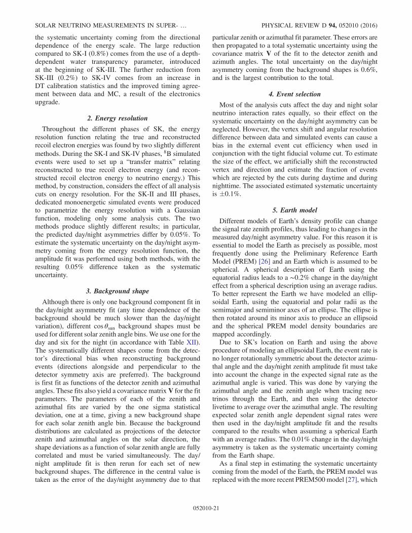
the systematic uncertainty coming from the directionaldependence of the energy scale. The large reductioncompared to SK-I (0.8%) comes from the use of a depth-dependent water transparency parameter, introducedat the beginning of SK-III. The further reduction fromSK-III (0.2%) to SK-IV comes from an increase inDT calibration statistics and the improved timing agree-ment between data and MC, a result of the electronicsupgrade.

2. Energy resolution

Throughout the different phases of SK, the energyresolution function relating the true and reconstructedrecoil electron energies was found by two slightly differentmethods. During the SK-I and SK-IV phases, 8B simulatedevents were used to set up a “transfer matrix” relatingreconstructed to true recoil electron energy (and recon-structed recoil electron energy to neutrino energy.) Thismethod, by construction, considers the effect of all analysiscuts on energy resolution. For the SK-II and III phases,dedicated monoenergetic simulated events were producedto parametrize the energy resolution with a Gaussianfunction, modeling only some analysis cuts. The twomethods produce slightly different results; in particular,the predicted day/night asymmetries differ by 0.05%. Toestimate the systematic uncertainty on the day/night asym-metry coming from the energy resolution function, theamplitude fit was performed using both methods, with theresulting 0.05% difference taken as the systematicuncertainty.

3. Background shape

Although there is only one background component fit inthe day/night asymmetry fit (any time dependence of thebackground should be much slower than the day/nightvariation), different cos θsun background shapes must beused for different solar zenith angle bins. We use one for theday and six for the night (in accordance with Table XII).The systematically different shapes come from the detec-tor’s directional bias when reconstructing backgroundevents (directions alongside and perpendicular to thedetector symmetry axis are preferred). The backgroundis first fit as functions of the detector zenith and azimuthalangles. These fits also yield a covariance matrixV for the fitparameters. The parameters of each of the zenith andazimuthal fits are varied by the one sigma statisticaldeviation, one at a time, giving a new background shapefor each solar zenith angle bin. Because the backgrounddistributions are calculated as projections of the detectorzenith and azimuthal angles on the solar direction, theshape deviations as a function of solar zenith angle are fullycorrelated and must be varied simultaneously. The day/night amplitude fit is then rerun for each set of newbackground shapes. The difference in the central value istaken as the error of the day/night asymmetry due to that

particular zenith or azimuthal fit parameter. These errors arethen propagated to a total systematic uncertainty using thecovariance matrix V of the fit to the detector zenith andazimuth angles. The total uncertainty on the day/nightasymmetry coming from the background shapes is 0.6%,and is the largest contribution to the total.

4. Event selection

Most of the analysis cuts affect the day and night solarneutrino interaction rates equally, so their effect on thesystematic uncertainty on the day/night asymmetry can beneglected. However, the vertex shift and angular resolutiondifference between data and simulated events can cause abias in the external event cut efficiency when used inconjunction with the tight fiducial volume cut. To estimatethe size of the effect, we artificially shift the reconstructedvertex and direction and estimate the fraction of eventswhich are rejected by the cuts during daytime and duringnighttime. The associated estimated systematic uncertaintyis �0.1%.

5. Earth model

Different models of Earth’s density profile can changethe signal rate zenith profiles, thus leading to changes in themeasured day/night asymmetry value. For this reason it isessential to model the Earth as precisely as possible, mostfrequently done using the Preliminary Reference EarthModel (PREM) [26] and an Earth which is assumed to bespherical. A spherical description of Earth using theequatorial radius leads to a ∼0.2% change in the day/nighteffect from a spherical description using an average radius.To better represent the Earth we have modeled an ellip-soidal Earth, using the equatorial and polar radii as thesemimajor and semiminor axes of an ellipse. The ellipse isthen rotated around its minor axis to produce an ellipsoidand the spherical PREM model density boundaries aremapped accordingly.Due to SK’s location on Earth and using the above

procedure of modeling an ellipsoidal Earth, the event rate isno longer rotationally symmetric about the detector azimu-thal angle and the day/night zenith amplitude fit must takeinto account the change in the expected signal rate as theazimuthal angle is varied. This was done by varying theazimuthal angle and the zenith angle when tracing neu-trinos through the Earth, and then using the detectorlivetime to average over the azimuthal angle. The resultingexpected solar zenith angle dependent signal rates werethen used in the day/night amplitude fit and the resultscompared to the results when assuming a spherical Earthwith an average radius. The 0.01% change in the day/nightasymmetry is taken as the systematic uncertainty comingfrom the Earth shape.As a final step in estimating the systematic uncertainty

coming from the model of the Earth, the PREM model wasreplaced with the more recent PREM500model [27], which


052010-21

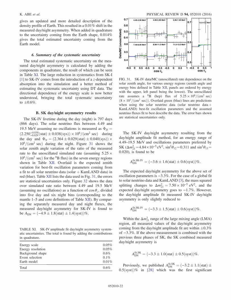
gives an updated and more detailed description of thedensity profile of Earth. This resulted in a 0.01% shift in themeasured day/night asymmetry. When added in quadratureto the uncertainty coming from the Earth shape, 0.014%gives the total estimated uncertainty coming from theEarth model.

6. Summary of the systematic uncertainty

The total estimated systematic uncertainty on the mea-sured day/night asymmetry is calculated by adding thecomponents in quadrature, the result of which can be seenin Table XI. The large reduction in systematics from SK-I[1] to SK-IV comes from the introduction of a z-dependentabsorption into the simulation and a better method ofestimating the systematic uncertainty using DT data. Thedirectional dependence of the energy scale is now betterunderstood, bringing the total systematic uncertaintyto �0.6%.

B. SK day/night asymmetry results

The SK-IV livetime during the day (night) is 797 days(866 days). The solar neutrino flux between 4.49 and19.5 MeV assuming no oscillations is measured as ΦD ¼ð2.250þ0.030

−0.029ðstatÞ � 0.038ðsysÞÞ × 106=ðcm2 secÞ duringthe day and ΦN ¼ ð2.364� 0.029ðstatÞ � 0.040ðsysÞÞ ×106=ðcm2 secÞ during the night. Figure 31 shows thesolar zenith angle variation of the ratio of the measuredrate to the unoscillated simulated rate (assuming 5.25 ×106=ðcm2 secÞ for the 8B flux) in the seven energy regionsshown in Table XII. Overlaid is the expected zenithvariation for best-fit oscillation parameters coming froma fit to all solar neutrino data (solar þ KamLAND data) inred (blue). Table XII lists the data used in Fig. 31, the errorsare statistical uncertainties only. Figure 32 shows the dataover simulated rate ratio between 4.49 and 19.5 MeV(assuming no oscillations) as a function of cos θz, dividedinto five day and six night bins (corresponding to themantle 1–5 and core definitions of Table XII). By compar-ing the separately measured day and night fluxes, themeasured day/night asymmetry for SK-IV is found tobe ADN ¼ ð−4.9� 1.8ðstatÞ � 1.4ðsystÞÞ%.

The SK-IV day/night asymmetry resulting from theday/night amplitude fit method, for an energy range of4.49–19.5 MeV and oscillations parameters preferred bySK (Δm2

21¼4.84×10−5 eV2, sin2θ12¼0.311 and sin2θ13¼0.020), is found to be

Afit;SK-IVDN ¼ ð−3.6� 1.6ðstatÞ � 0.6ðsystÞÞ%:

The expected day/night asymmetry for the above set ofoscillation parameters is −3.3%. For the case of a global fitto solar neutrino data and KamLAND [3], the mass squaredsplitting changes to Δm2

21 ¼ 7.50 × 10−5 eV2, and theexpected day/night asymmetry goes to −1.7%. However,the day/night amplitude fit measured SK-IV day/nightasymmetry is only slightly reduced to

Afit;SK-IVDN ¼ ð−3.3� 1.5ðstatÞ � 0.6ðsystÞÞ%:

Within the Δm221 range of the large mixing angle (LMA)

region, all measured values of the day/night asymmetrycoming from the day/night amplitude fit are within �0.3%of −3.3%. If the above measurement is combined with theprevious three phases of SK, the SK combined measuredday/night asymmetry is

Afit;SKDN ¼ ð−3.3� 1.0ðstatÞ � 0.5ðsystÞÞ%:

Previously, we published Afit;SKDN ¼ ð−3.2� 1.1ðstatÞ �

0.5ðsystÞÞ% in [28] which was the first significant

TABLE XI. SK-IV amplitude fit day/night asymmetry system-atic uncertainties. The total is found by adding the contributionsin quadrature.

Energy scale 0.05%Energy resolution 0.05%Background shape 0.6%Event selection 0.1%Earth model 0.01%

Total 0.6%

0.4

0.5

0.6

0.7 4.49-4.99 MeV 4.99-5.99 MeV 5.99-7.49 MeV

0.4

0.5

0.6 7.49-8.99 MeV 8.99-11.0 MeV 11.0-13.0 MeV

1

0.3

0.4

0.5

0.6

0.7 13.0-15.5 MeV

Dat

a/M

C (

un

osc

illat

ed)

-0.5 0 0.5 -0.5 0 0.5 -0.5 0 0.5 1 -0.5 0 0.5

zθcos zθcos

FIG. 31. SK-IV data/MC (unoscillated) rate dependence on thesolar zenith angle, for various energy regions (zenith angle andenergy bins defined in Table XII, panels are ordered by energywith the upper, left panel being the lowest). The unoscillatedrate assumes a 8B (hep) flux of 5.25 × 106=ðcm2 secÞð8 × 103=ðcm2 secÞÞ. Overlaid green (blue) lines are predictionswhen using the solar neutrino data (solar neutrino dataþKamLAND) best-fit oscillation parameters and the assumedneutrino fluxes fit to best describe the data. The error bars shownare statistical uncertainties only.


052010-22

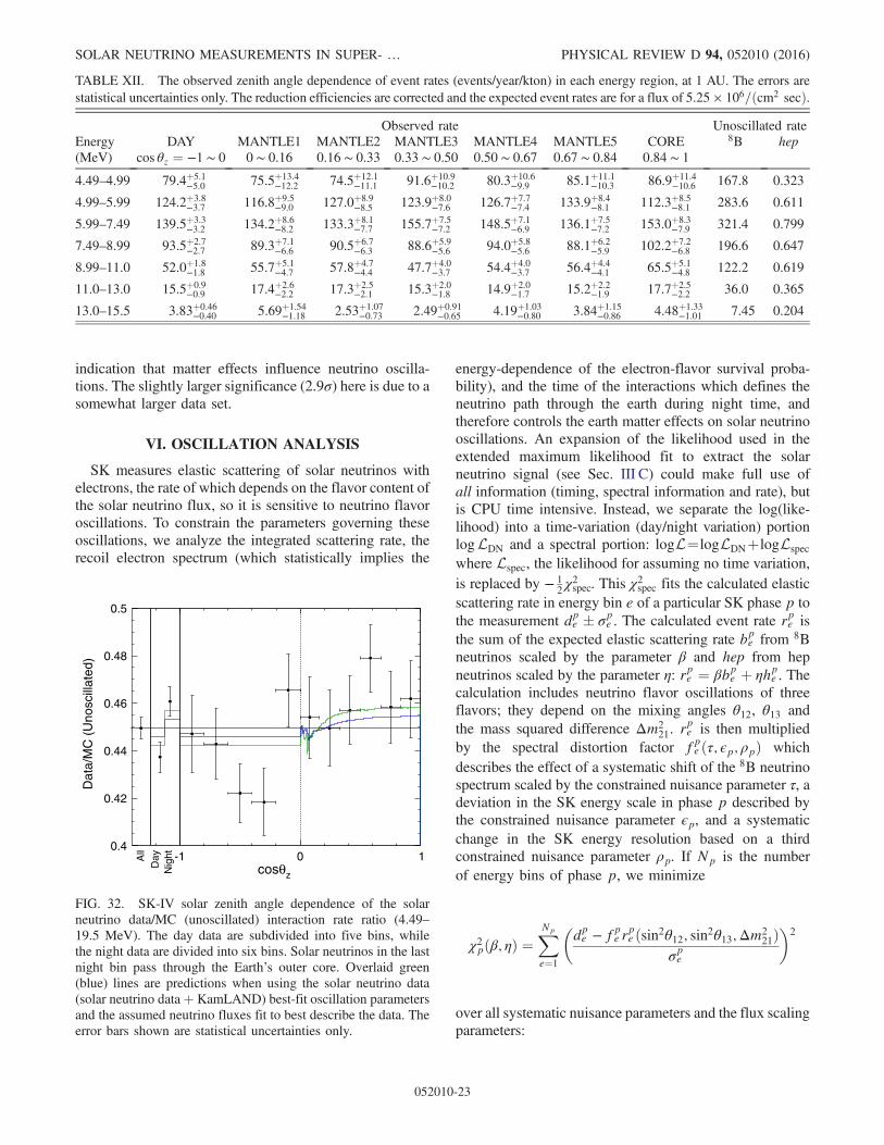
indication that matter effects influence neutrino oscilla-tions. The slightly larger significance (2.9σ) here is due to asomewhat larger data set.

VI. OSCILLATION ANALYSIS

SK measures elastic scattering of solar neutrinos withelectrons, the rate of which depends on the flavor content ofthe solar neutrino flux, so it is sensitive to neutrino flavoroscillations. To constrain the parameters governing theseoscillations, we analyze the integrated scattering rate, therecoil electron spectrum (which statistically implies the

energy-dependence of the electron-flavor survival proba-bility), and the time of the interactions which defines theneutrino path through the earth during night time, andtherefore controls the earth matter effects on solar neutrinooscillations. An expansion of the likelihood used in theextended maximum likelihood fit to extract the solarneutrino signal (see Sec. III C) could make full use ofall information (timing, spectral information and rate), butis CPU time intensive. Instead, we separate the log(like-lihood) into a time-variation (day/night variation) portionlogLDN and a spectral portion: logL¼logLDNþlogLspec

where Lspec, the likelihood for assuming no time variation,is replaced by − 1

2χ2spec. This χ2spec fits the calculated elastic

scattering rate in energy bin e of a particular SK phase p tothe measurement dpe � σpe . The calculated event rate rpe isthe sum of the expected elastic scattering rate bpe from 8Bneutrinos scaled by the parameter β and hep from hepneutrinos scaled by the parameter η: rpe ¼ βbpe þ ηhpe . Thecalculation includes neutrino flavor oscillations of threeflavors; they depend on the mixing angles θ12, θ13 andthe mass squared difference Δm2

21. rpe is then multiplied

by the spectral distortion factor fpe ðτ; ϵp; ρpÞ whichdescribes the effect of a systematic shift of the 8B neutrinospectrum scaled by the constrained nuisance parameter τ, adeviation in the SK energy scale in phase p described bythe constrained nuisance parameter ϵp, and a systematicchange in the SK energy resolution based on a thirdconstrained nuisance parameter ρp. If Np is the numberof energy bins of phase p, we minimize

χ2pðβ; ηÞ ¼XNp

e¼1

�dpe − fpe r

pe ðsin2θ12; sin2θ13;Δm2

21Þσpe

�2

over all systematic nuisance parameters and the flux scalingparameters:

TABLE XII. The observed zenith angle dependence of event rates (events/year/kton) in each energy region, at 1 AU. The errors arestatistical uncertainties only. The reduction efficiencies are corrected and the expected event rates are for a flux of 5.25 × 106=ðcm2 secÞ.

Observed rate Unoscillated rateEnergy DAY MANTLE1 MANTLE2 MANTLE3 MANTLE4 MANTLE5 CORE 8B hep(MeV) cos θz ¼ −1 ∼ 0 0 ∼ 0.16 0.16 ∼ 0.33 0.33 ∼ 0.50 0.50 ∼ 0.67 0.67 ∼ 0.84 0.84 ∼ 1

4.49–4.99 79.4þ5.1−5.0 75.5þ13.4

−12.2 74.5þ12.1−11.1 91.6þ10.9

−10.2 80.3þ10.6−9.9 85.1þ11.1

−10.3 86.9þ11.4−10.6 167.8 0.323

4.99–5.99 124.2þ3.8−3.7 116.8þ9.5

−9.0 127.0þ8.9−8.5 123.9þ8.0

−7.6 126.7þ7.7−7.4 133.9þ8.4

−8.1 112.3þ8.5−8.1 283.6 0.611

5.99–7.49 139.5þ3.3−3.2 134.2þ8.6

−8.2 133.3þ8.1−7.7 155.7þ7.5

−7.2 148.5þ7.1−6.9 136.1þ7.5

−7.2 153.0þ8.3−7.9 321.4 0.799

7.49–8.99 93.5þ2.7−2.7 89.3þ7.1

−6.6 90.5þ6.7−6.3 88.6þ5.9

−5.6 94.0þ5.8−5.6 88.1þ6.2

−5.9 102.2þ7.2−6.8 196.6 0.647

8.99–11.0 52.0þ1.8−1.8 55.7þ5.1

−4.7 57.8þ4.7−4.4 47.7þ4.0

−3.7 54.4þ4.0−3.7 56.4þ4.4

−4.1 65.5þ5.1−4.8 122.2 0.619

11.0–13.0 15.5þ0.9−0.9 17.4þ2.6

−2.2 17.3þ2.5−2.1 15.3þ2.0

−1.8 14.9þ2.0−1.7 15.2þ2.2

−1.9 17.7þ2.5−2.2 36.0 0.365

13.0–15.5 3.83þ0.46−0.40 5.69þ1.54

−1.18 2.53þ1.07−0.73 2.49þ0.91

−0.65 4.19þ1.03−0.80 3.84þ1.15

−0.86 4.48þ1.33−1.01 7.45 0.204

cosθz

Dat

a/M

C (

Uno

scill

ated

)

All

Day

Nig

ht

0.4-1 0 1

0.42

0.44

0.46

0.48

0.5

FIG. 32. SK-IV solar zenith angle dependence of the solarneutrino data/MC (unoscillated) interaction rate ratio (4.49–19.5 MeV). The day data are subdivided into five bins, whilethe night data are divided into six bins. Solar neutrinos in the lastnight bin pass through the Earth’s outer core. Overlaid green(blue) lines are predictions when using the solar neutrino data(solar neutrino dataþ KamLAND) best-fit oscillation parametersand the assumed neutrino fluxes fit to best describe the data. Theerror bars shown are statistical uncertainties only.


052010-23

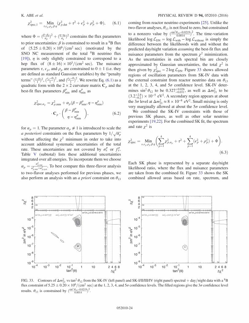
χ2spec;1 ¼ Minτ;ϵp;ρp;β;η

ðχ2p;dat þ τ2 þ ϵ2p þ ρ2p þ ΦÞ; ð6:1Þ

where Φ ¼ ðβ−β0σβÞ2 þ ðη−η0ση

Þ2 constrains the flux parameters

to prior uncertainties: β is constrained to result in a 8B fluxof ð5.25� 0.20Þ × 106=ðcm2 secÞ (motivated by theSNO NC measurement of the total 8B neutrino flux[19]), η is only slightly constrained to correspond to ahep flux of ð8� 16Þ × 103=ðcm2 secÞ. The nuisanceparameters τ, ϵp, and ρp are constrained to 0� 1 (i.e. theyare defined as standard Gaussian variables) by the “penalty

terms” ðτ−01Þ2, ðϵp−0

1Þ2, and ðρp−0

1Þ2. We rewrite Eq. (6.1) as a

quadratic form with the 2 × 2 curvature matrix Cp and thebest-fit flux parameters βpmin and ηpmin as

χ2spec;αp ¼ χ2p;min þ αpðβ − βpmin; η − ηpminÞ

· Cp ·�β − βpmin

η − ηpmin

�; ð6:2Þ

for αp ¼ 1. The parameter αp ≠ 1 is introduced to scale thea posteriori constraints on the flux parameters by 1= ffiffiffiffiffi

αpp

without affecting the χ2 minimum in order to take intoaccount additional systematic uncertainties of the totalrate. These uncertainties are not covered by σpe or fpe .Table V (subtotal) lists these additional uncertaintiesintegrated over all energies. To incorporate them we choose

αp ¼ σ2p;statσ2p;statþσ2p;syst

. To best compare this three-flavor analysis

to two-flavor analyses performed for previous phases, wealso perform an analysis with an a priori constraint on θ13

coming from reactor neutrino experiments [25]. Unlike thetwo-flavor analyses, θ13 is not fixed to zero, but constrained

to a nonzero value by ðsin2θ13−0.02190.0014 Þ2. The time-variation

likelihood logLDN ¼ logLwith − logLwithout is simply thedifference between the likelihoods with and without thepredicted day/night variation assuming the best-fit flux andnuisance parameters from the spectrum χ2 minimization.As the uncertainties in each spectral bin are closelyapproximated by Gaussian uncertainties, the total χ2 isthen given by χ2spec − 2 logLDN. Figure 33 shows allowedregions of oscillation parameters from SK-IV data withthe external constraint from reactor neutrino data on θ13at the 1, 2, 3, 4, and 5σ confidence level. SK-IV deter-mines sin2 θ12 to be 0.327þ0.026

−0.031 , as well as Δm221 to be

ð3.2þ2.8−0.2Þ × 10−5 eV2. A secondary region appears at about

the 3σ level at Δm221 ≈ 8 × 10−8 eV2. Small mixing is only

very marginally allowed at about the 5σ confidence level.We combined the SK-IV constraints with those of

previous SK phases, as well as other solar neutrinoexperiments [19,22]. For the combined SK fit, the spectrumand rate χ2 is

χ2spec ¼ Minν;ϵp;ρp;β;η

�X4p¼1

χ2p;αp þ τ2 þX4p¼1

ðϵ2p þ ρ2pÞ þ Φ

�:

ð6:3Þ

Each SK phase is represented by a separate day/nightlikelihood ratio, where the flux and nuisance parametersare taken from the combined fit. Figure 33 shows the SKcombined allowed areas based on rate, spectrum, and

sin2(Θ13)=0.0219±0.0014sin2(Θ12)=0.327+0.026

-0.031 Δm221=(3.2+2.8

-0.2) 10-5eV2

Δm2 in

eV

2

10-9

10-8

10-7

10-6

10-5

10-4

2 4 6 8

1σ 2σ 3σ

Δχ2tan2(θ)10

-410

-310

-210

-11 10

2468

1σ

2σ

3σ

Δχ2

sin2(Θ13)=0.0219±0.0014sin2(Θ12)=0.334+0.027

-0.023 Δm221=(4.8+1.5

-0.8) 10-5eV2

Δm2 in

eV

2

10-9

10-8

10-7

10-6

10-5

10-4

2 4 6 8

1σ 2σ 3σ

Δχ 2tan2(θ)10

-410

-310

-210

-11 10

2468

1σ

2σ

3σ

Δχ2

FIG. 33. Contours of Δm221 vs tan

2 θ12 from the SK-IV (left panel) and SK-I/II/III/IV (right panel) spectralþ day=night data with a 8Bflux constraint of 5.25� 0.20 × 106=ðcm2 secÞ at the 1, 2, 3, 4, and 5σ confidence levels. The filled regions give the 3σ confidence levelresults. θ13 is constrained by ðsin2 θ13−0.0219

0.0014 Þ2.


052010-24

day/night variation. SK selects largemixing (0.5>sin2θ12>0.2) over small mixing by more than five standarddeviations and very strongly (3.6σ) favors the Δm2

21 ofthe LMA solution (below 2 × 10−4 eV2 and above2 × 10−5 eV2) over any other oscillation parameters. SKdetermines sin2 θ12 to be 0.334þ0.027

−0.023 , as well as Δm221 to

be ð4.8þ1.5−0.8Þ × 10−5 eV2.

Figure 34 compares the SKþ SNO combined con-straints to those based on SNO data alone [19]. WhileSNO’s measurement of the mixing angle is more precise(sin2θ12 ¼ 0.299þ0.023

−0.020 ) than SK’s, its Δm221 constraints are

poorer [ð5.6þ1.9−1.4Þ × 10−5 eV2]. Also, SNO very slightly

favors the low mass (Low) solution (region near 10−7 eV2)and allows small mixing at the 3.6σ level. The combinedanalysis of SK and SNO is particularly powerful: as SNOand SK both measure 8B neutrinos in a very similar energyrange but in a different way and with different systematiceffects, the combined analysis profits from correlations andis better than a mere addition of χ2 ’s. The SKþ SNOcombined analysis measures sin2 θ12 ¼ 0.310� 0.014 andΔm2

21 ¼ ð4.8þ1.3−0.6Þ × 10−5 eV2. Oscillation parameter val-

ues outside the LMA are very strongly excluded: the solarmixing angle lies within 0.12 ≤ sin2 θ12 ≤ 0.45 at about the7.5σ C.L., Δm2

21 < 1.33 × 10−5 eV2 (which includes the“small mixing angle” and “low mass” regions) is ruledout at the 5.5σ C.L., and Δm2

21>1.9×10−4 eV2 is excludedat 7.5σ C.L. The hep flux constraint used by SNO isð7.9� 1.2Þ × 103=ðcm2 secÞ from the solar standard model[21]. The SK and SNO combined analysis also uses thistighter constraint.

The combined allowed contours based on SK, SNO[19] and other solar neutrino experiments’ [22] data,KamLAND’s constraints and the combination of the twoare shown in Figs. 34 and 35. SK and SNO dominatethe combined fit to all solar neutrino data. This can beseen from the two almost identical sets of greencontours in Fig. 34. The low energy measurement ofthe 7Be day/night asymmetry [29] does not change the

sin2(Θ13)=0.0219±0.0014sin2(Θ12)=0.310±0.014 Δm2

21=(4.8+1.3 -0.6) 10-5eV2

Δ m2 in

eV

2

10-9

10-8

10-7

10-6

10-5

10-4

2 4 6 81σ 2σ 3σ

Δχ2tan2(θ)

10-4

10-3

10-2

10-1

1 10

2468

1σ

2σ

3σ

Δχ2

sin2(Θ13)=0.0219±0.0014

sin2(Θ12)=0.307+0.013 -0.012 Δm2

21=(7.49+0.19 -0.18) 10-5eV2

sin2(Θ12)=0.308±0.014 Δm221=(4.85+1.33

-0.59) 10-5eV2sin2(Θ12)=0.316+0.034

-0.026 Δm221=(7.54+0.19

-0.18) 10-5eV2

Δm2 in

10-5

eV2

123456789

101112131415161718

2 4 6 8

1σ 2σ 3σ

Δχ2sin2(θ12)

0.1 0.2 0.3 0.4 0.5

2468

1σ

2σ

3σ

Δχ2

FIG. 34. Left: comparison of the oscillation parameter determination of the SK and SNO combined analysis (red) to the oscillationconstraints of SNO by itself (blue). Right: allowed contours of Δm2

21 vs sin2 θ12 from solar neutrino data (green), KamLAND data(blue), and the combined result (red). For comparison, the almost identical result of the SKþ SNO combined fit is shown by the dasheddotted lines. The filled regions give the 3σ confidence level results, the other contours shown are at the 1 and 2σ confidence level (for the

solar analyses, 4 and 5σ confidence level contours are also displayed). θ13 is constrained by ðsin2 θ13−0.02190.0014 Þ2.

sin2(Θ12)=0.309+0.014 -0.013 sin2(Θ13)=0.028±0.015

sin2(Θ12)=0.310+0.022 -0.017 sin2(Θ13)=0.027+0.024

-0.027

sin2(Θ12)=0.326+0.044 -0.037 sin2(Θ13)=0.010+0.033

-0.034

sin2 (Θ

13)

0.0

0.1

0.2

2 4 6 81σ 2σ 3σ

Δχ2sin2(Θ12)0.0 0.1 0.2 0.3 0.4 0.5

2468

1σ

2σ

3σ

Δχ2

FIG. 35. Allowed contours of sin2 θ13 vs sin2 θ12 from solarneutrino data (green) at 1, 2, 3, 4, and 5σ and KamLANDmeasurements (blue) at the 1, 2, and 3σ confidence levels. Alsoshown is the combined result in red. The yellow band is the θ13measurement from reactor neutrino data [25].


052010-25

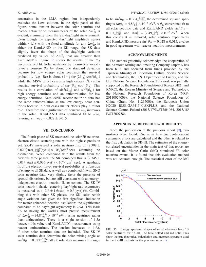
constraints in the LMA region, but independentlyexcludes the Low solution. In the right panel of thisfigure, some tension between the solar neutrino andreactor antineutrino measurements of the solar Δm2

21 isevident, stemming from the SK day/night measurement.Even though the expected day/night amplitude agreeswithin ∼1.1σ with the fitted amplitude for any Δm2

21, ineither the KamLAND or the SK range, the SK dataslightly favor the shape of the day/night variationpredicted by values of Δm2

21 that are smaller thanKamLAND’s. Figure 35 shows the results of the θ13unconstrained fit. Solar neutrinos by themselves weaklyfavor a nonzero θ13 by about one standard deviationbecause for low energy solar neutrinos the survivalprobability (e.g 7Be) is about ð1 − 1

2sin2ð2θ12ÞÞcos4ðθ13Þ

while the MSW effect causes a high energy (8B) solarneutrino survival probability of sin2ðθ12Þ cos4ðθ13Þ. Thisresults in a correlation of sin2ðθ12Þ and sin2ðθ13Þ forhigh energy neutrinos and an anticorrelation for lowenergy neutrinos. KamLAND reactor neutrino data hasthe same anticorrelation as the low energy solar neu-trinos because in both cases matter effects play a minorrole. Therefore the significance of nonzero θ13 increasesin the solar þ KamLAND data combined fit to ∼2σ,favoring sin2 θ13 ¼ 0.028� 0.015.

VII. CONCLUSION

The fourth phase of SK measured the solar 8B neutrino-electron elastic scattering-rate with the highest precisionyet. SK-IV measured a solar neutrino flux of ð2.308�0.020ðstatÞþ0.039

−0.040ðsystÞÞ × 106=ðcm2 secÞ assuming nooscillations. When combined with the results from theprevious three phases, the SK combined flux is ð2.345�0.014ðstatÞ � 0.036ðsystÞÞ × 106=ðcm2 secÞ. A quadraticfit of the electron-flavor survival probability as a functionof energy to all SK data, as well as a combined fit with SNOsolar neutrino data, very slightly favor the presence ofspectral distortions, but are still consistent with an energy-independent electron neutrino flavor content. The SK-IVsolar neutrino elastic scattering day/night rate asymmetryis measured as ð−3.6� 1.6ðstatÞ � 0.6ðsystÞÞ%. Combi-ning this with other SK phases, the SK solar zenithangle variation data gives the first significant indicationfor matter-enhanced neutrino oscillation: the significancecompared to no day/night asymmetry is 2.9σ. This leadsSK to having the world’s most precise measurementof Δm2

21 ¼ ð4.8þ1.5−0.8Þ × 10−5 eV2, using neutrinos rather

than antineutrinos. There is a slight tension of 1.5σbetween this value and KamLAND’s measurement usingreactor antineutrinos. The tension increases to 1.6σ,if other solar neutrino data are included. The SK-IVsolar neutrino data determine the solar mixing angle assin2θ12 ¼ 0.327þ0.026

−0.031 , all SK solar data measures this angle

to be sin2θ12 ¼ 0.334þ0.027−0.023 , the determined squared split-

ting is Δm221 ¼ 4.8þ1.5

−0.8 × 10−5 eV2. A θ13 constrained fit toall solar neutrino data and KamLAND yields sin2 θ12 ¼0.307þ0.013

−0.012 and Δm221 ¼ ð7.49þ0.19

−0.18Þ × 10−5 eV2. Whenthis constraint is removed, solar neutrino experimentsand KamLAND measure sin2 θ13 ¼ 0.028� 0.015, a valuein good agreement with reactor neutrino measurements.

ACKNOWLEDGMENTS

The authors gratefully acknowledge the cooperation ofthe Kamioka Mining and Smelting Company. Super-K hasbeen built and operated from funds provided by theJapanese Ministry of Education, Culture, Sports, Scienceand Technology, the U.S. Department of Energy, and theU.S. National Science Foundation. This work was partiallysupported by the Research Foundation of Korea (BK21 andKNRC), the Korean Ministry of Science and Technology,the National Research Foundation of Korea (NRF-20110024009), the National Science Foundation ofChina (Grant No. 11235006), the European UnionH2020 RISE-GA641540-SKPLUS, and the NationalScience Centre, Poland (2015/17/N/ST2/04064, 2015/18/E/ST200758).

APPENDIX A: REVISED SK-III RESULTS

Since the publication of the previous report [9], twomistakes were found. One is in how energy-dependentsystematic errors are calculated and the other is related tothe flux calculation in SK-III. The estimates of the energy-correlated uncertainties in the main text of that report arebased on the Monte Carlo (MC) simulated 8B solarneutrino events. It is found that this evaluation methodwas not accurate enough. The statistical error of the MC

Total electron energy [MeV]0 2 4 6 8 10 12 14

Arb

itra

ry u

nit

0

20

40

60

80

100

120

140

160

310×True spectrum

Spectrum for the previous SK-III

FIG. 36. Energy spectrum shapes of recoil electrons from 8Bsolar neutrinos for SK-III. The blue dotted and red solid linesshow the true theoretical calculation and incorrect spectrum usedin the SK-III analysis in the previous report [9].


052010-26

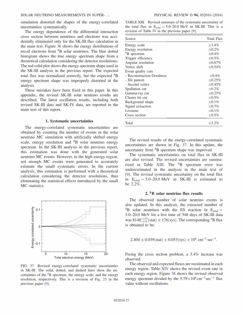
simulation distorted the shapes of the energy-correlateduncertainties systematically.The energy dependence of the differential interaction

cross section between neutrinos and electrons was acci-dentally eliminated only for the SK-III flux calculation inthe main text. Figure 36 shows the energy distributions ofrecoil electrons from 8B solar neutrinos. The blue dottedhistogram shows the true energy spectrum shape from atheoretical calculation considering the detector resolutions.The red solid plot shows the energy spectrum shape used inthe SK-III analysis in the previous report. The expectedtotal flux was normalized correctly, but the expected 8Benergy spectrum shape was improperly distorted in theanalysis.These mistakes have been fixed in this paper. In this

appendix, the revised SK-III solar neutrino results aredescribed. The latest oscillation results, including bothrevised SK-III data and SK-IV data, are reported in themain text of this report.

1. Systematic uncertainties

The energy-correlated systematic uncertainties areobtained by counting the number of events in the solarneutrino MC simulation with artificially shifted energyscale, energy resolution and 8B solar neutrino energyspectrum. In the SK-III analysis in the previous report,this estimation was done with the generated solarneutrino MC events. However, in the high energy region,not enough MC events were generated to accuratelyestimate the small systematic errors. In the currentanalysis, this estimation is performed with a theoreticalcalculation considering the detector resolutions, thuseliminating the statistical effects introduced by the smallMC statistics.

The revised results of the energy-correlated systematicuncertainties are shown in Fig. 37. In this update, theuncertainty from 8B spectrum shape was improved.The systematic uncertainties on total flux in SK-III

are also revised. The revised uncertainties are summa-rized in Table XIII. The 8B spectrum error wasunderestimated in the analysis in the main text of[9]. The revised systematic uncertainty on the total fluxin Etotal ¼ 5.0–20.0 MeV in SK-III is estimated tobe 2.2%.

2. 8B solar neutrino flux results

The observed number of solar neutrino events isalso updated. In this analysis, the extracted number of8B solar neutrinos with the ES reaction in Etotal ¼5.0–20.0 MeV for a live time of 548 days of SK-III datawas 8148þ133

−131ðstatÞ � 176ðsysÞ. The corresponding 8B fluxis obtained to be:

2.404� 0.039ðstatÞ � 0.053ðsysÞ × 106 cm−2 sec−1:

Fixing the cross section problem, a 3.4% increase wasobserved.The observed and expected fluxes are reestimated in each

energy region. Table XIV shows the revised event rate ineach energy region. Figure 38 shows the revised observedenergy spectrum divided by the 5.79×106 cm−2sec−1 fluxvalue without oscillations.

TABLE XIII Revised summary of the systematic uncertainty ofthe total flux in Etotal ¼ 5.0–20.0 MeV in SK-III. This is arevision of Table IV in the previous paper [9].

Source Total Flux

Energy scale �1.4%Energy resolution �0.2%8B spectrum �0.4%Trigger efficiency �0.5%Angular resolution �0.67%Vertex shift �0.54%Event quality cuts- Reconstruction Goodness �0.4%- Hit pattern �0.25%- Second vertex �0.45%Spallation cut �0.2%Gamma-ray cut �0.25%Cluster hit cut �0.5%Background shape �0.1%Signal extraction �0.7%Livetime �0.1%Cross section �0.5%

Total �2.2%

-0.1

0

0.1

5 10 15 20Total electron energy (MeV)

Ene

rgy

corr

elat

ed u

ncer

tain

ty

FIG. 37 Revised energy-correlated systematic uncertaintiesin SK-III. The solid, dotted, and dashed lines show the un-certainties of the 8B spectrum, the energy scale, and the energyresolution, respectively. This is a revision of Fig. 25 in theprevious paper [9].


052010-27

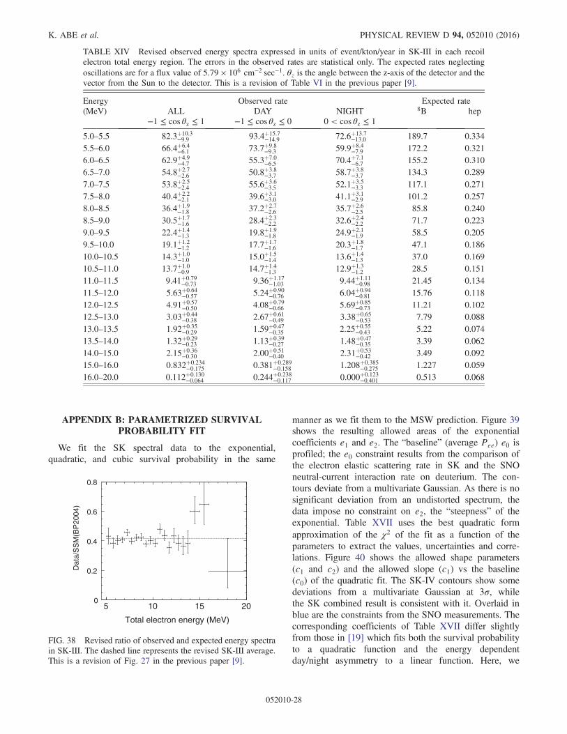
APPENDIX B: PARAMETRIZED SURVIVALPROBABILITY FIT

We fit the SK spectral data to the exponential,quadratic, and cubic survival probability in the same

manner as we fit them to the MSW prediction. Figure 39shows the resulting allowed areas of the exponentialcoefficients e1 and e2. The “baseline” (average Pee) e0 isprofiled; the e0 constraint results from the comparison ofthe electron elastic scattering rate in SK and the SNOneutral-current interaction rate on deuterium. The con-tours deviate from a multivariate Gaussian. As there is nosignificant deviation from an undistorted spectrum, thedata impose no constraint on e2, the “steepness” of theexponential. Table XVII uses the best quadratic formapproximation of the χ2 of the fit as a function of theparameters to extract the values, uncertainties and corre-lations. Figure 40 shows the allowed shape parameters(c1 and c2) and the allowed slope (c1) vs the baseline(c0) of the quadratic fit. The SK-IV contours show somedeviations from a multivariate Gaussian at 3σ, whilethe SK combined result is consistent with it. Overlaid inblue are the constraints from the SNO measurements. Thecorresponding coefficients of Table XVII differ slightlyfrom those in [19] which fits both the survival probabilityto a quadratic function and the energy dependentday/night asymmetry to a linear function. Here, we

0

0.2

0.4

0.6

0.8

5 10 15 20

Total electron energy (MeV)

Dat

a/S

SM

(BP

2004

)

FIG. 38 Revised ratio of observed and expected energy spectrain SK-III. The dashed line represents the revised SK-III average.This is a revision of Fig. 27 in the previous paper [9].

TABLE XIV Revised observed energy spectra expressed in units of event/kton/year in SK-III in each recoilelectron total energy region. The errors in the observed rates are statistical only. The expected rates neglectingoscillations are for a flux value of 5.79 × 106 cm−2 sec−1. θz is the angle between the z-axis of the detector and thevector from the Sun to the detector. This is a revision of Table VI in the previous paper [9].

Energy Observed rate Expected rate(MeV) ALL DAY NIGHT 8B hep

−1 ≤ cos θz ≤ 1 −1 ≤ cos θz ≤ 0 0 < cos θz ≤ 1

5.0–5.5 82.3þ10.3−9.9 93.4þ15.7

−14.9 72.6þ13.7−13.0 189.7 0.334

5.5–6.0 66.4þ6.4−6.1 73.7þ9.8

−9.3 59.9þ8.4−7.9 172.2 0.321

6.0–6.5 62.9þ4.9−4.7 55.3þ7.0

−6.5 70.4þ7.1−6.7 155.2 0.310

6.5–7.0 54.8þ2.7−2.6 50.8þ3.8

−3.7 58.7þ3.8−3.7 134.3 0.289

7.0–7.5 53.8þ2.5−2.4 55.6þ3.6

−3.5 52.1þ3.5−3.3 117.1 0.271

7.5–8.0 40.4þ2.2−2.1 39.6þ3.1

−3.0 41.1þ3.1−2.9 101.2 0.257

8.0–8.5 36.4þ1.9−1.8 37.2þ2.7

−2.6 35.7þ2.6−2.5 85.8 0.240

8.5–9.0 30.5þ1.7−1.6 28.4þ2.3

−2.2 32.6þ2.4−2.2 71.7 0.223

9.0–9.5 22.4þ1.4−1.3 19.8þ1.9

−1.8 24.9þ2.1−1.9 58.5 0.205

9.5–10.0 19.1þ1.2−1.2 17.7þ1.7

−1.6 20.3þ1.8−1.7 47.1 0.186

10.0–10.5 14.3þ1.0−1.0 15.0þ1.5

−1.4 13.6þ1.4−1.3 37.0 0.169

10.5–11.0 13.7þ1.0−0.9 14.7þ1.4

−1.3 12.9þ1.3−1.2 28.5 0.151

11.0–11.5 9.41þ0.79−0.73 9.36þ1.17

−1.03 9.44þ1.11−0.98 21.45 0.134

11.5–12.0 5.63þ0.64−0.57 5.24þ0.90

−0.76 6.04þ0.94−0.81 15.76 0.118

12.0–12.5 4.91þ0.57−0.50 4.08þ0.79

−0.66 5.69þ0.85−0.73 11.21 0.102

12.5–13.0 3.03þ0.44−0.38 2.67þ0.61

−0.49 3.38þ0.65−0.53 7.79 0.088

13.0–13.5 1.92þ0.35−0.29 1.59þ0.47

−0.35 2.25þ0.55−0.43 5.22 0.074

13.5–14.0 1.32þ0.29−0.23 1.13þ0.39

−0.27 1.48þ0.47−0.35 3.39 0.062

14.0–15.0 2.15þ0.36−0.30 2.00þ0.51

−0.40 2.31þ0.53−0.42 3.49 0.092

15.0–16.0 0.832þ0.234−0.175 0.381þ0.289

−0.158 1.208þ0.385−0.275 1.227 0.059

16.0–20.0 0.112þ0.130−0.064 0.244þ0.238

−0.117 0.000þ0.123−0.401 0.513 0.068


052010-28

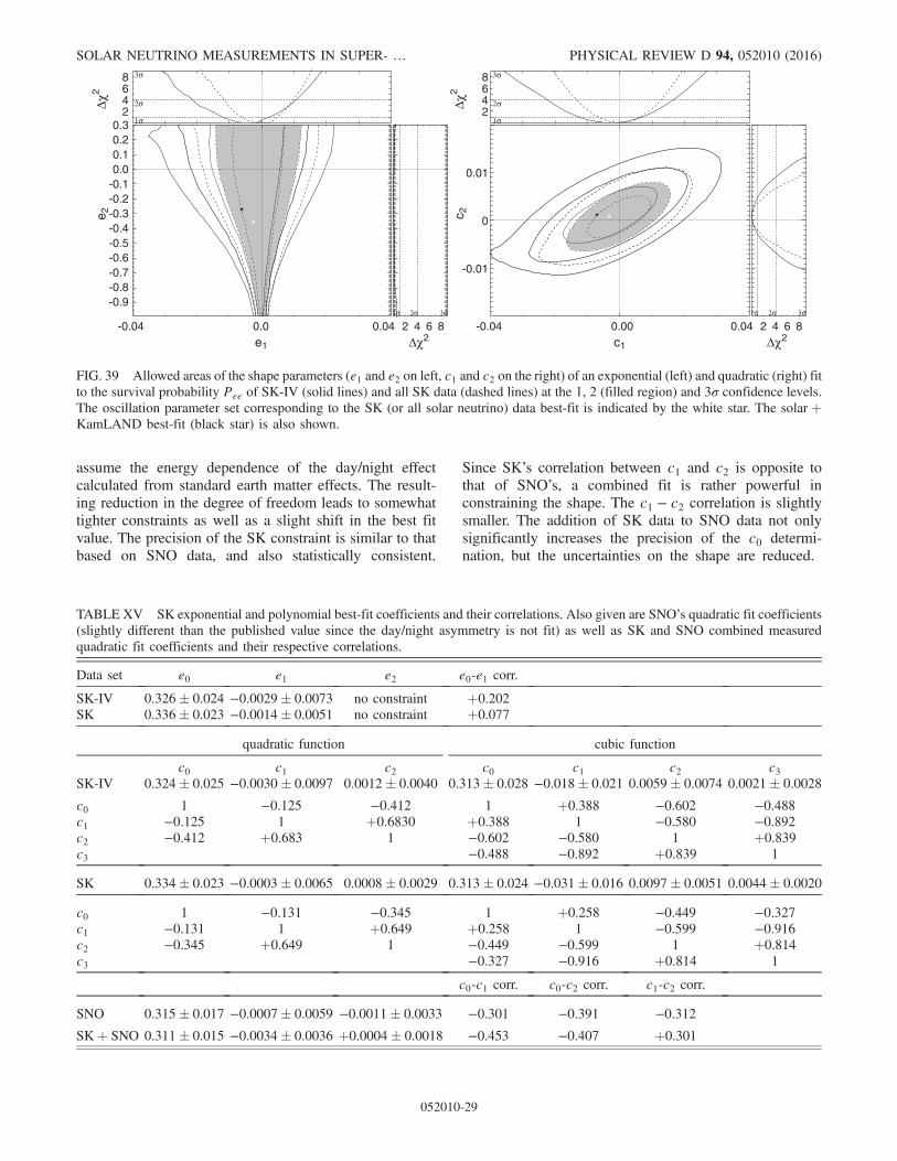
assume the energy dependence of the day/night effectcalculated from standard earth matter effects. The result-ing reduction in the degree of freedom leads to somewhattighter constraints as well as a slight shift in the best fitvalue. The precision of the SK constraint is similar to thatbased on SNO data, and also statistically consistent.

Since SK’s correlation between c1 and c2 is opposite tothat of SNO’s, a combined fit is rather powerful inconstraining the shape. The c1 − c2 correlation is slightlysmaller. The addition of SK data to SNO data not onlysignificantly increases the precision of the c0 determi-nation, but the uncertainties on the shape are reduced.

e 2

-0.9 -0.8 -0.7 -0.6 -0.5 -0.4 -0.3 -0.2 -0.1 0.0 0.1 0.2 0.3

2 4 6 81σ 2σ 3σ

Δχ2e1

-0.04 0.0 0.04

2468

1σ

2σ

3σ

Δχ2

c 2

-0.01

0

0.01

2 4 6 81σ 2σ 3σ

Δχ2c1

-0.04 0.00 0.04

2468

1σ

2σ

3σ

Δχ2

FIG. 39 Allowed areas of the shape parameters (e1 and e2 on left, c1 and c2 on the right) of an exponential (left) and quadratic (right) fitto the survival probability Pee of SK-IV (solid lines) and all SK data (dashed lines) at the 1, 2 (filled region) and 3σ confidence levels.The oscillation parameter set corresponding to the SK (or all solar neutrino) data best-fit is indicated by the white star. The solar þKamLAND best-fit (black star) is also shown.

TABLE XV SK exponential and polynomial best-fit coefficients and their correlations. Also given are SNO’s quadratic fit coefficients(slightly different than the published value since the day/night asymmetry is not fit) as well as SK and SNO combined measuredquadratic fit coefficients and their respective correlations.

Data set e0 e1 e2 e0-e1 corr.

SK-IV 0.326� 0.024 −0.0029� 0.0073 no constraint þ0.202SK 0.336� 0.023 −0.0014� 0.0051 no constraint þ0.077

quadratic function cubic function

c0 c1 c2 c0 c1 c2 c3SK-IV 0.324� 0.025 −0.0030� 0.0097 0.0012� 0.0040 0.313� 0.028 −0.018� 0.021 0.0059� 0.0074 0.0021� 0.0028

c0 1 −0.125 −0.412 1 þ0.388 −0.602 −0.488c1 −0.125 1 þ0.6830 þ0.388 1 −0.580 −0.892c2 −0.412 þ0.683 1 −0.602 −0.580 1 þ0.839c3 −0.488 −0.892 þ0.839 1

SK 0.334� 0.023 −0.0003� 0.0065 0.0008� 0.0029 0.313� 0.024 −0.031� 0.016 0.0097� 0.0051 0.0044� 0.0020

c0 1 −0.131 −0.345 1 þ0.258 −0.449 −0.327c1 −0.131 1 þ0.649 þ0.258 1 −0.599 −0.916c2 −0.345 þ0.649 1 −0.449 −0.599 1 þ0.814c3 −0.327 −0.916 þ0.814 1

c0-c1 corr. c0-c2 corr. c1-c2 corr.

SNO 0.315� 0.017 −0.0007� 0.0059 −0.0011� 0.0033 −0.301 −0.391 −0.312SKþ SNO 0.311� 0.015 −0.0034� 0.0036 þ0.0004� 0.0018 −0.453 −0.407 þ0.301


052010-29

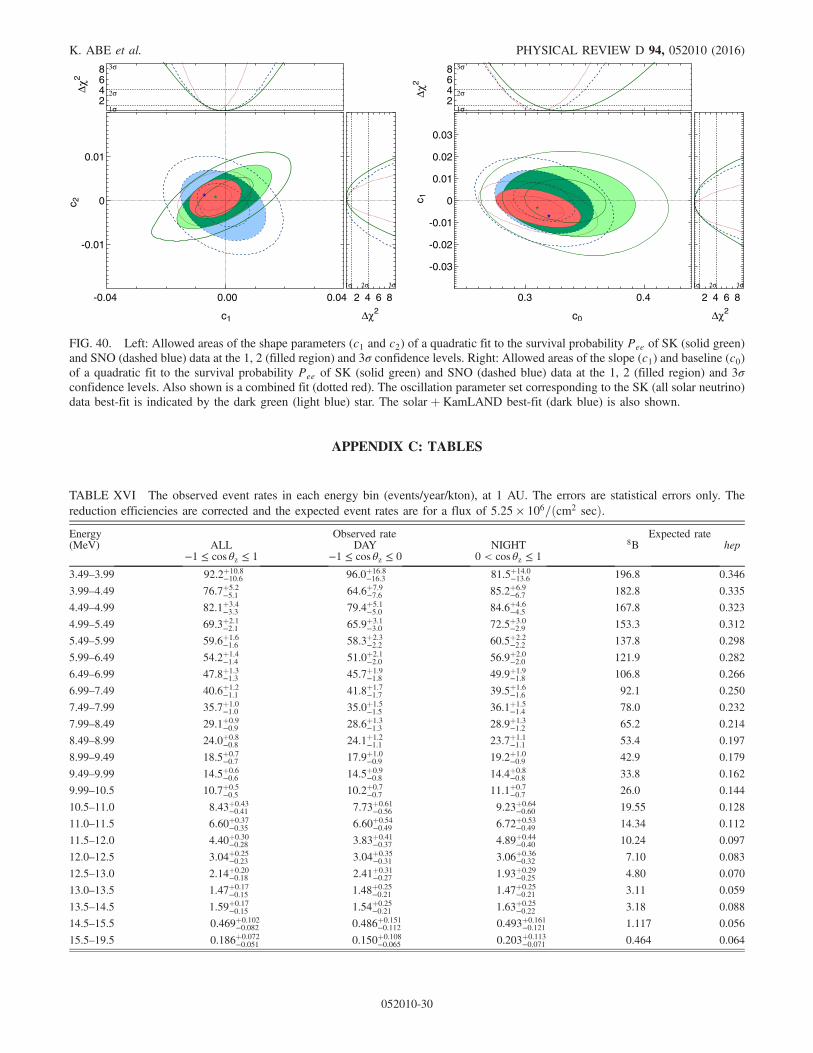
APPENDIX C: TABLES

c 2

-0.01

0

0.01

2 4 6 81σ 2σ 3σ

Δχ2c1

-0.04 0.00 0.04

2468

1σ

2σ

3σ

Δχ2

c 1

-0.03

-0.02

-0.01

0

0.01

0.02

0.03

2 4 6 81σ 2σ 3σ

Δχ2c0

0.3 0.4

2468

1σ

2σ

3σ

Δχ2

FIG. 40. Left: Allowed areas of the shape parameters (c1 and c2) of a quadratic fit to the survival probability Pee of SK (solid green)and SNO (dashed blue) data at the 1, 2 (filled region) and 3σ confidence levels. Right: Allowed areas of the slope (c1) and baseline (c0)of a quadratic fit to the survival probability Pee of SK (solid green) and SNO (dashed blue) data at the 1, 2 (filled region) and 3σconfidence levels. Also shown is a combined fit (dotted red). The oscillation parameter set corresponding to the SK (all solar neutrino)data best-fit is indicated by the dark green (light blue) star. The solar þ KamLAND best-fit (dark blue) is also shown.

TABLE XVI The observed event rates in each energy bin (events/year/kton), at 1 AU. The errors are statistical errors only. Thereduction efficiencies are corrected and the expected event rates are for a flux of 5.25 × 106=ðcm2 secÞ.Energy Observed rate Expected rate(MeV) ALL DAY NIGHT 8B hep

−1 ≤ cos θz ≤ 1 −1 ≤ cos θz ≤ 0 0 < cos θz ≤ 1

3.49–3.99 92.2þ10.8−10.6 96.0þ16.8

−16.3 81.5þ14.0−13.6 196.8 0.346

3.99–4.49 76.7þ5.2−5.1 64.6þ7.9

−7.6 85.2þ6.9−6.7 182.8 0.335

4.49–4.99 82.1þ3.4−3.3 79.4þ5.1

−5.0 84.6þ4.6−4.5 167.8 0.323

4.99–5.49 69.3þ2.1−2.1 65.9þ3.1

−3.0 72.5þ3.0−2.9 153.3 0.312

5.49–5.99 59.6þ1.6−1.6 58.3þ2.3

−2.2 60.5þ2.2−2.2 137.8 0.298

5.99–6.49 54.2þ1.4−1.4 51.0þ2.1

−2.0 56.9þ2.0−2.0 121.9 0.282

6.49–6.99 47.8þ1.3−1.3 45.7þ1.9

−1.8 49.9þ1.9−1.8 106.8 0.266

6.99–7.49 40.6þ1.2−1.1 41.8þ1.7

−1.7 39.5þ1.6−1.6 92.1 0.250

7.49–7.99 35.7þ1.0−1.0 35.0þ1.5

−1.5 36.1þ1.5−1.4 78.0 0.232

7.99–8.49 29.1þ0.9−0.9 28.6þ1.3

−1.3 28.9þ1.3−1.2 65.2 0.214

8.49–8.99 24.0þ0.8−0.8 24.1þ1.2

−1.1 23.7þ1.1−1.1 53.4 0.197

8.99–9.49 18.5þ0.7−0.7 17.9þ1.0

−0.9 19.2þ1.0−0.9 42.9 0.179

9.49–9.99 14.5þ0.6−0.6 14.5þ0.9

−0.8 14.4þ0.8−0.8 33.8 0.162

9.99–10.5 10.7þ0.5−0.5 10.2þ0.7

−0.7 11.1þ0.7−0.7 26.0 0.144

10.5–11.0 8.43þ0.43−0.41 7.73þ0.61

−0.56 9.23þ0.64−0.60 19.55 0.128

11.0–11.5 6.60þ0.37−0.35 6.60þ0.54

−0.49 6.72þ0.53−0.49 14.34 0.112

11.5–12.0 4.40þ0.30−0.28 3.83þ0.41

−0.37 4.89þ0.44−0.40 10.24 0.097

12.0–12.5 3.04þ0.25−0.23 3.04þ0.35

−0.31 3.06þ0.36−0.32 7.10 0.083

12.5–13.0 2.14þ0.20−0.18 2.41þ0.31

−0.27 1.93þ0.29−0.25 4.80 0.070

13.0–13.5 1.47þ0.17−0.15 1.48þ0.25

−0.21 1.47þ0.25−0.21 3.11 0.059

13.5–14.5 1.59þ0.17−0.15 1.54þ0.25

−0.21 1.63þ0.25−0.22 3.18 0.088

14.5–15.5 0.469þ0.102−0.082 0.486þ0.151

−0.112 0.493þ0.161−0.121 1.117 0.056

15.5–19.5 0.186þ0.072−0.051 0.150þ0.108

−0.065 0.203þ0.113−0.071 0.464 0.064


052010-30

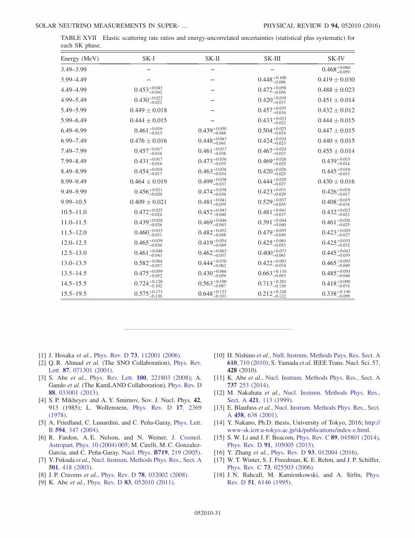
[1] J. Hosaka et al., Phys. Rev. D 73, 112001 (2006).[2] Q. R. Ahmad et al. (The SNO Collaboration), Phys. Rev.

Lett. 87, 071301 (2001).[3] S. Abe et al., Phys. Rev. Lett. 100, 221803 (2008); A.

Gando et al. (The KamLAND Collaboration), Phys. Rev. D88, 033001 (2013).

[4] S. P. Mikheyev and A. Y. Smirnov, Sov. J. Nucl. Phys. 42,913 (1985); L. Wolfenstein, Phys. Rev. D 17, 2369(1978).

[5] A. Friedland, C. Lunardini, and C. Peña-Garay, Phys. Lett.B 594, 347 (2004).

[6] R. Fardon, A. E. Nelson, and N. Weiner, J. Cosmol.Astropart. Phys. 10 (2004) 005; M. Cirelli, M. C. Gonzalez-Garcia, and C. Peña-Garay, Nucl. Phys. B719, 219 (2005).

[7] Y. Fukuda et al., Nucl. Instrum. Methods Phys. Res., Sect. A501, 418 (2003).

[8] J. P. Cravens et al., Phys. Rev. D 78, 032002 (2008).[9] K. Abe et al., Phys. Rev. D 83, 052010 (2011).

[10] H. Nishino et al., Null. Instrum. Methods Pays. Res. Sect. A610, 710 (2010); S. Yamada et al. IEEE Trans. Nucl. Sci. 57,428 (2010).

[11] K. Abe et al., Nucl. Instrum. Methods Phys. Res., Sect. A737 253 (2014).

[12] M. Nakahata et al., Nucl. Instrum. Methods Phys. Res.,Sect. A 421, 113 (1999).

[13] E. Blaufuss et al., Nucl. Instrum. Methods Phys. Res., Sect.A 458, 638 (2001).

[14] Y. Nakano, Ph.D. thesis, University of Tokyo, 2016; http://www‑sk.icrr.u‑tokyo.ac.jp/sk/publications/index‑e.html.

[15] S.W. Li and J. F. Beacom, Phys. Rev. C 89, 045801 (2014),Phys. Rev. D 91, 105005 (2015).

[16] Y. Zhang et al., Phys. Rev. D 93, 012004 (2016).[17] W. T. Winter, S. J. Freedman, K. E. Rehm, and J. P. Schiffer,

Phys. Rev. C 73, 025503 (2006).[18] J. N. Bahcall, M. Kamionkowski, and A. Sirlin, Phys.

Rev. D 51, 6146 (1995).

TABLE XVII Elastic scattering rate ratios and energy-uncorrelated uncertainties (statistical plus systematic) foreach SK phase.

Energy (MeV) SK-I SK-II SK-III SK-IV

3.49–3.99 − − − 0.468þ0.060−0.059

3.99–4.49 − − 0.448þ0.100−0.096 0.419� 0.030

4.49–4.99 0.453þ0.043−0.042 − 0.472þ0.058

−0.056 0.488� 0.023

4.99–5.49 0.430þ0.023−0.022 − 0.420þ0.039

−0.037 0.451� 0.014

5.49–5.99 0.449� 0.018 − 0.457þ0.035−0.034 0.432� 0.012

5.99–6.49 0.444� 0.015 − 0.433þ0.023−0.022 0.444� 0.015

6.49–6.99 0.461þ0.016−0.015 0.439þ0.050

−0.048 0.504þ0.025−0.024 0.447� 0.015

6.99–7.49 0.476� 0.016 0.448þ0.043−0.041 0.424þ0.024

−0.023 0.440� 0.015

7.49–7.99 0.457þ0.017−0.016 0.461þ0.037

−0.036 0.467þ0.024−0.023 0.455� 0.014

7.99–8.49 0.431þ0.017−0.016 0.473þ0.036

−0.035 0.469þ0.026−0.025 0.439þ0.015

−0.014

8.49–8.99 0.454þ0.018−0.017 0.463þ0.036

−0.034 0.420þ0.026−0.025 0.445þ0.016

−0.015

8.99–9.49 0.464� 0.019 0.499þ0.038−0.037 0.444þ0.029

−0.027 0.430� 0.016

9.49–9.99 0.456þ0.021−0.020 0.474þ0.038

−0.036 0.423þ0.031−0.029 0.426þ0.018

−0.017

9.99–10.5 0.409� 0.021 0.481þ0.041−0.039 0.529þ0.037

−0.035 0.408þ0.019−0.018

10.5–11.0 0.472þ0.025−0.024 0.452þ0.043

−0.040 0.481þ0.041−0.037 0.432þ0.023

−0.021

11.0–11.5 0.439þ0.028−0.026 0.469þ0.046

−0.043 0.391þ0.044−0.040 0.461þ0.026

−0.025

11.5–12.0 0.460þ0.033−0.031 0.482þ0.052

−0.048 0.479þ0.055−0.049 0.423þ0.029

−0.027

12.0–12.5 0.465þ0.039−0.036 0.419þ0.054

−0.049 0.425þ0.061−0.053 0.425þ0.035

−0.032

12.5–13.0 0.461þ0.048−0.043 0.462þ0.063

−0.057 0.400þ0.073−0.061 0.445þ0.043

−0.039

13.0–13.5 0.582þ0.064−0.057 0.444þ0.070

−0.062 0.422þ0.093−0.074 0.465þ0.055

−0.049

13.5–14.5 0.475þ0.059−0.052 0.430þ0.066

−0.059 0.663þ0.110−0.093 0.485þ0.054

−0.048

14.5–15.5 0.724þ0.120−0.102 0.563þ0.100

−0.087 0.713þ0.201−0.150 0.418þ0.090

−0.074

15.5–19.5 0.575þ0.173−0.130 0.648þ0.123

−0.103 0.212þ0.248−0.122 0.338þ0.140

−0.099


052010-31


http://dx.doi.org/10.1103/PhysRevLett.87.071301







http://dx.doi.org/10.1016/j.physletb.2004.05.047


http://dx.doi.org/10.1088/1475-7516/2004/10/005

http://dx.doi.org/10.1088/1475-7516/2004/10/005

http://dx.doi.org/10.1016/j.nuclphysb.2005.04.034

http://dx.doi.org/10.1016/S0168-9002(03)00425-X

http://dx.doi.org/10.1016/S0168-9002(03)00425-X



http://dx.doi.org/10.1109/TNS.2009.2034854

http://dx.doi.org/10.1109/TNS.2009.2034854

http://dx.doi.org/10.1016/j.nima.2013.11.081

http://dx.doi.org/10.1016/j.nima.2013.11.081

http://dx.doi.org/10.1016/S0168-9002(98)01200-5

http://dx.doi.org/10.1016/S0168-9002(98)01200-5

http://dx.doi.org/10.1016/S0168-9002(00)00900-1

http://dx.doi.org/10.1016/S0168-9002(00)00900-1

http://www-sk.icrr.u-tokyo.ac.jp/sk/publications/index-e.html







http://dx.doi.org/10.1103/PhysRevC.89.045801






[19] B. Aharmin et al., Phys. Rev. C 88, 025501 (2013).[20] B. Aharmim et al., Astrophys. J. 653, 1545 (2006).[21] J. N. Bahcall, A. M. Serenelli, and S. Basu, Astrophys. J.

Suppl. Ser. 165, 400 (2006).[22] R. Davis, Jr., D. S. Harmer, and K. C. Hoffman (Homestake

Experiment), Phys. Rev. Lett. 20, 1205 (1968); J. N.Abdurashitov et al. (SAGE collaboration), Phys. Rev. C80, 015807 (2009); M. Altmann et al. (GALLEX Collabo-ration), Phys. Lett. B 616, 174 (2005); G. Bellini et al.(Borexino Collaboration), Phys. Rev. Lett. 107, 141302(2011).

[23] Bellini et al. Phys. Rev. D 82, 033006 (2010); Phys. Rev.Lett. 108, 051302 (2012).

[24] M. B. Smy et al., Phys. Rev. D 69, 011104(R)(2004).

[25] F. P. An et al. (Daya Bay Collaboration), Chin. Phys. C 37,011001 (2013); J. K. Ahn et al., Phys. Rev. Lett. 108,191802 (2012); Y. Abe et al., Phys. Rev. D 86, 052008(2012).

[26] A. M. Dziewonski and D. L. Anderson, Phys. Earth Planet.Inter. 25, 297 (1981).

[27] J. J. Durek and G. Ekstrom, Bull. Seismol. Soc. Am. 86, 144(1996).

[28] A. Renshaw et al., Phys. Rev. Lett. 112, 091805(2014).

[29] G. Bellini et al., Phys. Lett. B 707, 22 (2012).


052010-32


http://dx.doi.org/10.1086/508768

http://dx.doi.org/10.1086/504043

http://dx.doi.org/10.1086/504043












http://dx.doi.org/10.1088/1674-1137/37/1/011001

http://dx.doi.org/10.1088/1674-1137/37/1/011001





http://dx.doi.org/10.1016/0031-9201(81)90046-7

http://dx.doi.org/10.1016/0031-9201(81)90046-7




solar neutrino measurements in super … a measurement of this oscillation parameter. it is also...

Documents