C a r d i f f U n i v e r s i t y

S h a i n a l S u t a r i a

0 7 7 6 1 3 0 9 7 0 9

1 2 / 1 / 2 0 1 0

c1059965 The lab performed in soil mechanics was divided into two parts in the first one the compressibility and the one dimensional consolidation of speswhite kaolin was found out . A specific soil specimen was prepared in the lab and load was applied on the soil specimen so that the layer is compressed and excess water is drained out which happened in an interval of time . The dial guage reading was noted down for different time interval. The graph was plotted down and coefficient of consolidation and volume change was found. In the second experiment of permeability and flow nets the constant head permeameter test was carried out in which for each reading the flow rate the volume of flow and time was recorded also the flow rate of the flow tank model was noted down and also a flownet is drawn after the experiment the difference between the experimental volumetric flow rate and the theoretical flow rate difference is noted down .

Soil Mechanics(SM)

Table of Contents One dimensional Consolidation .................................................................................................... 3

Introduction : ........................................................................................................................... 3

Theory: ..................................................................................................................................... 3

Compressiblity ��: ......................................................................................................................... 3

One dimensional consolidation ....................................................................................................... 3

Calculation of consolidation equation: ........................................................................................... 4

Procedure: ................................................................................................................................ 5

Calculations and results : .......................................................................................................... 6

Compression data:........................................................................................................................... 6

Consolidation data: ......................................................................................................................... 6

DIAL GAUGE READING VS SQUARE ROOT OF TIME......................................................................... 7

Discussion: ............................................................................................................................... 8

Validity of one dimensional consolidation ................................................................................. 8

PERMEABILITY AND FLOW NETS ................................................................................................... 9

Introduction: ............................................................................................................................ 9

Theory: ..................................................................................................................................... 9

Flow nets: ...................................................................................................................................... 10

Procedure: .............................................................................................................................. 11

Calculations and results: ......................................................................................................... 12

Calculation of permeability: .......................................................................................................... 13

Calculations: ........................................................................................................................... 14

Discussion: ............................................................................................................................. 14

References: ................................................................................................................................ 15

One dimensional Consolidation

Introduction : Consolidation is the rate of volume change with time- giving time to produce an amount of settlement required. The process of consolidation comprises the gradual reduction of volume of a fully saturated soil with times as water is squeezed out of the pore spaces in the soil due to load applied on the soil. This load which produces this effect is known as the consolidation pressure.

Theory:

Compressiblity ��: Volume changes in the soil occurs because the volume of void changes. They are defined by the ratio:

Void ratio=volume of voids/volume of solids

Effective stress is the stress seated in the mineral grain structure or soil skeleton so if it changes the soil skeleton will respond by decreasing and increasing in volume as water is squeezed out of or drawn into the void spaces.

These are recoverable or irrecoverable components of volume changes in the soil skeleton and it is postulated that these are due to

1. Rearrangement of soil particles- permanent or irrecoverable 2. Elastic strains in the particles – these are recoverable 3. Compression of bound water layers –these are recoverable

All three components will produce volume decreases but 2 and 3 will only provide a volume increase

One dimensional consolidation considers the rate at which the water comes out of the soil and also determines rates of:

• Volume change in the soil

• Settlements at the surface of the soil • Pore pressure dissipation with time

Several assumptions are made such as soil is homogenous and fully saturated and the solid particles and the pore water are incompressible. The other assumptions made were

• Compression and flow were one dimensional • Darcy’s law was applied to all hydraulic gradients though at low gradients deviation may

occur

• The coefficient of volume change remains constant during this experiment although when they decrease during consolidation

• The load is applied over the whole soil layer though the loads are applied over a construction period and usually do not extend over a wide area in comparison with the thickness of the consolidating deposit.

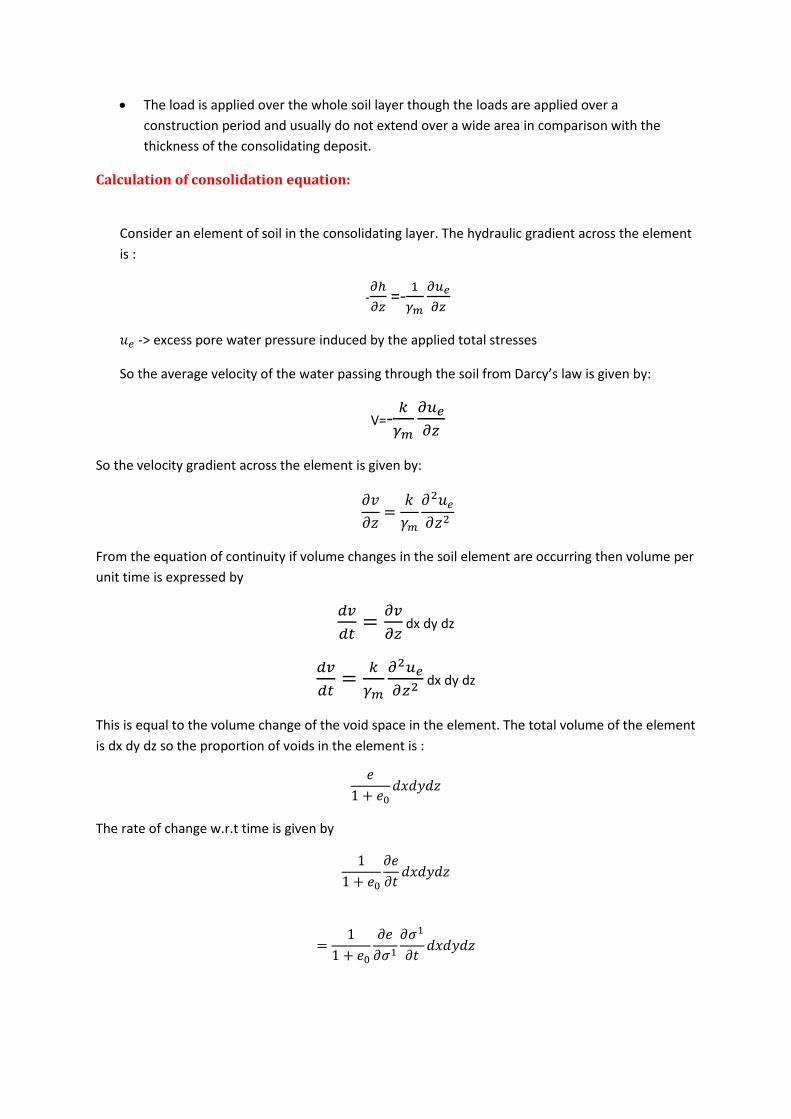
Calculation of consolidation equation:

Consider an element of soil in the consolidating layer. The hydraulic gradient across the element is :

-����

=-�

��

�

��

�� -> excess pore water pressure induced by the applied total stresses

So the average velocity of the water passing through the soil from Darcy’s law is given by:

V=-

��

�

��

So the velocity gradient across the element is given by:

����

��

��

����

���

From the equation of continuity if volume changes in the soil element are occurring then volume per unit time is expressed by

����

� ����

dx dy dz

����

� ��

��

��� dx dy dz

This is equal to the volume change of the void space in the element. The total volume of the element is dx dy dz so the proportion of voids in the element is :

�� � ��

��� ��

The rate of change w.r.t time is given by

�� � ��

���"

��� ��

��

� � ��

���#�

�#�

�"��� ��

� $%����

�"��� ��

This concludes the rate of increase of effective stress being equal to rate of dissipation of the excess pore pressure ��

Equating equations we get

���

�"�

�%���

����

��� � &�����

���

Where

&�- > coefficient of consolidation

%� ->coefficient of compressibility (volume change )

K -> coefficient of permeability

Therefore the dimensionless time factor is given by

'� �&�"

�(

Procedure: • In this experiment the sample was produced in the laboratory different in the way

where the undisturbed sample is taken from the ground. • Loading is applied through the loading yoke or load hanger and a counter balanced

lever system with a load ratio of around 10:1 so that a relatively small mass on the hanger can produce the large stresses required on the specimen.

• Also an initial pressure is applied to return the specimen to near its in situ effective stress to act as a starting point for reloading or swelling. This stress will depend on the stress history the soil has been subjected to.

• The pressure increment requires 72 min of application time with different times in the order such that the consolidation coefficient can be calculated.

• The stop watch was started and the effective at every reading required the pressure was noted in the dial gauge.

• The graph was then plotted.

Calculations and results : Date Load

Multiplier Gauge factor Soil Initial height Diameter(mm)

10 0.002 Speswhite kaolin

19 100

Compression data: Hanger load(N)

Load on sample(N)

Applied pressure(KN/m2)

Final dial guage

Piston displacement

Equilibrium height

0 0 0 0 0 19 10 100 12.73 570 1.14 17.86 20 200 25.46 747 1.494 17.508

Consolidation data: Time (s) Time1/2

Min1/2 Dial guage

(-) Time(s) Time1/2

Min1/2 Dial Guage

(-)

0 0.00 570 540 3.00 664

10 0.41 590 735 3.50 678

20 0.58 595 960 4.00 690

30 0.71 598 1215 4.50 703

40 0.82 601 1500 5.00 713

50 0.91 604 1815 5.50 722

60 1.00 606 2160 6.00 729

90 1.22 613 2545 6.50 735

135 1.50 621 2940 7.00 740

184 1.75 628 3375 7.50 743

240 2.00 635 3840 8.00 746

375 2.50 651 4335 8.50 747

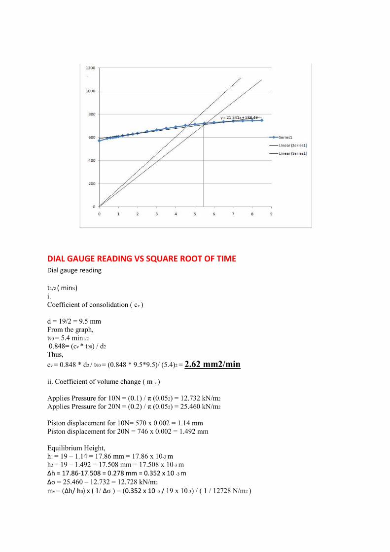
DIAL GAUGE READING VS SQUARE ROOT OF TIME Dial gauge reading t1/2 ( min½) i. Coefficient of consolidation ( cv ) d = 19/2 = 9.5 mm From the graph, t90 = 5.4 min1/2

0.848= (cv * t90) / d2

Thus, cv = 0.848 * d2 / t90 = (0.848 * 9.5*9.5)/ (5.4)2 = 2.62 mm2/min ii. Coefficient of volume change ( m v ) Applies Pressure for 10N = (0.1) / π (0.052) = 12.732 kN/m2

Applies Pressure for 20N = (0.2) / π (0.052) = 25.460 kN/m2

Piston displacement for 10N= 570 x 0.002 = 1.14 mm Piston displacement for 20N = 746 x 0.002 = 1.492 mm Equilibrium Height, h1 = 19 – 1.14 = 17.86 mm = 17.86 x 10-3 m h2 = 19 – 1.492 = 17.508 mm = 17.508 x 10-3 m Δh = 17.86-17.508 = 0.278 mm = 0.352 x 10 -3 m Δσ = 25.460 – 12.732 = 12.728 kN/m2

mv = (Δh/ h0) x ( 1/ Δσ ) = (0.352 x 10 -3 / 19 x 10-3) / ( 1 / 12728 N/m2 )

= 1.449 x 10-6 m2/N.

Discussion: Taylor showed that terzaghi theory of one dimensional consolidation gave a straight line when the

degree of consolidation was plotted against )'� at 60% and at 90% the theoretical curve was at 1.15

times the extrapolated straight line portion. The theory of consolidation relates only to pore water pressure dissipation and is referred to a primary consolidation. At the beginning an initial compression is produced by factors such as bedding of the porous discs and compression of air or gas that come out of the solution

• There is a second compression towards the end which is recorded as the continuing volume decrease even when after all the measurable pore pressures have been fully dissipated

The graph of the coefficient of consolidation is plotted in this way :

• Plot guage reading against the square root of time • Draw a straight line from deflection at a gradient 1.15 times the gradient of the straight

portion of the experimental plot.

• Where the line cuts the experimental curve is considered to be the point at 90% of degree of consolidation.

• Determine the value of )"*� and hence t90, the time required to produce 90% of degree of

consolidation.

• The coeffient of consolidation ,Cv is then determined by

+�,'�*���

"*�

Here '�*�=0.848 and d is the average length of drainage path for the load increment Validity of one dimensional consolidation

Several assumptions are made such as soil is homogenous and fully saturated and the solid particles and the pore water are incompressible. The other assumptions made were

• Compression and flow were one dimensional • Darcy’s law was applied to all hydraulic gradients though at low gradients deviation may

occur

• The coefficient of volume change remains constant during this experiment although when they decrease during consolidation

• The load is applied over the whole soil layer though the loads are applied over a construction period and usually do not extend over a wide area in comparison with the thickness of the consolidating deposit.

• No secondry compression or creep occurs.If this occurs the void ratio-effective stress relationship is not solely dependent on the consolidation process

PERMEABILITY AND FLOW NETS

Introduction: As a result of hydrological cycle it is inevitable that the voids between soil particles will fill with water until they become fully saturated. To effectively allow for this in design and analysis, knowledge of the coefficient of permeability of the media encountered is required as well as the hydraulic potentials or heads which they are subjected.

Theory: • Pressure and head :

Pressure is the force per unit area acting at a point in water. Head is the measure of pressure but in terms of a height. The total head at a point is given by the bernaulli’s equation

H=hz+-.+��

�/

Where H->Total head hz->position head -.->piezometric head

��

�/-> Velocity head

The velocity head can be ignored as the velocity of flow of water through soil is quite small.

• Darcy’s law:

This states that the discharge velocity, v of water is proportional to the hydraulic gradient,i .

01

=v=ki

Where k->Darcy coefficient of permeability

The hydraulic gradient i is the ratio of the head loss h over the distance l.

The coefficient of permeability k is dependent on the nature of the voids and the properties of the fluid, particularly its viscosity while the discharge velocity v is define as the quantity of water, q percolating through a cross-sectional area A in unit time.

Flow nets: When there is difference in hydraulic head either side of a water-retaining structure such as a dam or sheet-pile wall water will flow beneath and around the structure .Only an estimate of the flows or resulting water pressures can be obtained since this is the best our determinations of the coefficient of permeability will allow.

A flow net comprises a set of two types of lines

• Flow lines: These are paths along which water can flow in an crosssection.The intervals between adjacent flow lines represent a constant flow quantity so that the seepagw flow is by the quantity times by the no. Of flow channels.

• Equipotential lines: these are lines of equal level or equal total head

Flownet construction should have the following things:

• Should be at right angles • Should be square blocks

• Impermeable boundaries • Permeable boundaries –where a permeable soil boundary is in contact with open water as

on the upstream of the earth dam, this boundary will be equipotential.

Procedure: • The test is carried out by adjusting the control valve and waiting until the flow q through the

sample and the hydraulic head loss between the manometer points have reached a steady state.

• The flow rate q and head loss h are eventually measured and the coefficient of permeability is measured

• The test is repeated with different hydraulic gradients by adjusting the control valve to obtain a number of q and h values.

• The test is repeated three times with different flow volumes. 1000 cm3, 500 cm3 and 250 cm3. • For the flow net the length and the breadth of the tank are measured. Along with the height of

the water on either side of the cut of wall is aloes noted.

• Discharged water is emptied into a measuring cylinder, and the time taken to get the required volume of water discharged is noted.

• The step is repeated three times to the average of the time taken.

Calculations and results: Soil Type Fine sand

Distance between standpipes, l(cm) Diameter of permeameter, d(cm) 10 7.3

Area, A=41.833 &%�

Duration of Water Flow,

t(s)

Flow Volume q(cm3)

Potential head h1(cm)

Potential head 2, h2(cm)

Velocity v(cm/s)

Hydraulic gradient ,i

107 1000 66.0 37.4 0.223407

-2.86

68 500 75.4 53.2 0.176 -2.22

67 250 89.6 78.5 0.0891 -1.11

Here V=q/(A*t) i=��2�3

4

Length of the model (i.e. distance between the glass sides)(cm)

21

Measurement number Duration of water flow (s)

Flow volume(cm3) Flow rate (cm3/s)

1 110 1000 9.090 2 110 1000 9.090 3 109 1000 9.174 Average flow rate 9.118 Graph of v->i

Calculation of permeability:

k=7.34*�52� whose drainage characteristics are referred as good

y = -13.013x + 0.055

-3.5

-3

-2.5

-2

-1.5

-1

-0.5

0

0 0.05 0.1 0.15 0.2 0.25

V vs i

V vs i

Linear (V vs i)

Linear (V vs i)

Calculations: From the table, Average Flow rate = 9.118 cm3/s. From the flow net, Nf = 5 Nd = 11 h = 8-18.9 = - 10.9 cm b = 21 cm k = 7.34 x 10 -2 cm/s We know, Thus q = -(7.34 x 10 -2) x (5/11) x (- 10.9) x 21 = 7.637 cm3/s .

Discussion: • Thus the calculation of q came to be 7.637 cm3/s while the experimental result was found to

be 9.118 cm3/s with a difference of 1.8025 cm3/s . The error may occur due to inaccurate measurements of time and lengths of the pressure heads. Another reason for possible errors is the value used for the constant of permeability. As discussed the value we obtained from constant head permeameter may not be accurate. Even the inaccuracy of the flow drawn is a reason for any possible errors as drawn by hand the flow line and equipotential line are not appropriate and thus giving a inappropriate number of flow and equipotential line

• The constant head permeameter which is used to calculate the permeability of the soil is governed by the Darcy’s Law. The coefficient of permeability (k) was determined to be 7.34 x 10-2 which lies categories the sand as clean sand and clean gravel sand ( k lies between 10-2

and 10-5). However the values of k obtained may not be accurate due to possible factors. • According to Darcy’s law the forces in the fluid has to be in equilibrium with the visoisty of

the fluid which in turn is related to the volume. Thus if the volume changed there is affect of the permeameters. Another factor could be the presence of the biological life which alters the sample’s volume.

• The permeability of a soil is of great significance as it is the degree of flow of fluid through a soil. Thus it can be applied to calculate the seepage through earth dams embankments. It can also be helpful estimating settlements in foundation and slope stability analysis.

References:

i. BS 1377 : 5 : 1990 test 3 and test 5 ii. Soil Mechanics – Principle and practice ( Barnes ) iii. http://en.wikipedia.org/wiki/Flownet