soil indicators of changing land quality and capital value · soil indicators of changing land...
TRANSCRIPT

CSI ROAUST RALIA
CSIRO LAND and WATER
Soil indicators of changing landquality and capital value
A.J. Ringrose-Voase, G.W. Geeves, R.H. Merry and J.T. Wood
Technical Report No. 17/97

Soil indicators of changing landquality and capital value
A.J. Ringrose-VoaseCSIRO Land & Water, GPO Box 1666, Canberra ACT 2601
G.W. GeevesNSW Department of Land & Water Conservation, Cowra Research Centre, PO Box 445,Cowra NSW 2754
R.H. MerryCSIRO Land & Water, Private Bag No. 2, Glen Osmond SA 5064
J.T. WoodCSIRO Mathematical & Information Sciences, GPO Box 664, Canberra ACT 2601
Technical Report No. 17/97

Contact:Anthony Ringrose-VoaseCSIRO Land & WaterGPO Box 1666Canberra ACT 2601Telephone: 02-6246 5700e-mail: [email protected]
Disclaimer:Any recommendations contained in the publication do not necessarily representGRDC, LWRRDC or NAB policy. No person should act on the basis of the contents ofthis publication, whether as to matters of fact or opinion or other content, without firstobtaining specific, independent professional advice which confirms the informationcontained in this publication.
Publication data:Ringrose-Voase, A.J., Geeves, G.W., Merry, R.H. and Wood, J.T. 1997. Soil indica-tors of changing land quality and capital value. CSIRO (Australia) Land and WaterTechnical Report 17/97.

CSIRO Land & Water Technical Report 17/97
iii
ACKNOWLEDGMENTS
The project was financially supported by Grains Research and Development Corporation(GRDC), the Land and Water Resources Research and Development Corporation (LWRRDC)and the National Australia Bank. We are grateful to Colin Chartres, formerly of CSIRO Land& Water, Chris Shearer, formerly of the National Australia Bank, and Richard Price,LWRRDC, who initiated the project and subsequently supported it.
We are particularly grateful to the 37 farmers in the Wagga Wagga district who took part inthe study for allowing us to sample their paddocks and for providing paddock histories.
We thank Tom Green and Rod Drinkwater, CSIRO Land and Water, for invaluable assistancewith field and laboratory work.
We are grateful for advice and information received from John Brennan, Lloyd Davies, AlanKaiser, Nigel Phillips, Graham Stewart and Steve Sutherland of NSW Agriculture; AnthonyKrieg, ABARE; Nick Gazis, International Wool Secretariat; various agricultural merchants inWagga Wagga.
We also thank the following for participating in a workshop in Wagga Wagga in June 1995:
Chris ShearerBarry ColemanIan FergusonRichard HerbstDavid LynchGeorge SimpsonBruce StanfordRobert Tamblyn
National AustraliaBank
John Dore Bernard HartTim Hutchings
Farmers/Consultants
Colin Chartres CSIRO Land & Water
Keith HelyarTherese Hulme
NSW Agriculture
Nick LucasMichael PittBob Wynne
NSW Department ofLand and WaterConservation
Noel BeynonLois HuntLionel Wood
Department of PrimaryIndustries and Energy
Peta Ngale Landcare Foundation
Finally, we are indebted to Dermot McKane for his invaluable help in interpreting the soils ofthe Wagga Wagga 1:100,000 Map Sheet (McKane and Chen, 1997).

CSIRO Land & Water Technical Report 17/97
iv
CONTENTS
Acknowledgments ................................................................................................................... iii
Contents ....................................................................................................................................iv
Executive summary...................................................................................................................1
Background ...............................................................................................................................3Land value and soil degradation.............................................................................................3Finance industry perspective ..................................................................................................3Land quality assessment.........................................................................................................4
Aims............................................................................................................................................5
Methods......................................................................................................................................5Site selection ..........................................................................................................................6Soil sampling and analyses.....................................................................................................7Paddock productivity assessment...........................................................................................8
Livestock gross margin......................................................................................................8Crop income ......................................................................................................................9Variable costs ..................................................................................................................10
Data analysis.........................................................................................................................11Database..........................................................................................................................11Statistical analysis...........................................................................................................11
Results ......................................................................................................................................13Results for all soil-landscape types ......................................................................................13Erosional Soil Landscapes (SLT 4)......................................................................................14Transferral Soil Landscapes (SLT 5) ...................................................................................15Aeolian Soil Landscapes (SLT 6) ........................................................................................16Alluvial and Gilgai Soil Landscapes (SLT 78) ....................................................................18Colour...................................................................................................................................20
Discussion ................................................................................................................................20Comparison of SLT productivity .........................................................................................20Effect of soil properties on productivity...............................................................................22
Soil acidity and aluminium..............................................................................................22Organic carbon ...............................................................................................................25Available phosphorus ......................................................................................................27Effective cation exchange capacity..................................................................................27
Present value of soil properties ............................................................................................28
Recommendations ...................................................................................................................31
Industry implications..............................................................................................................33
Conclusions..............................................................................................................................34
References................................................................................................................................35
Appendix 1 Gross margin spreadsheet .................................................................................36
Appendix 2 Gross margin calculation for model livestock enterprises..............................40Merino wethers.....................................................................................................................40

CSIRO Land & Water Technical Report 17/97
v
Self-replacing merino ewes..................................................................................................41Second-cross lambs..............................................................................................................42Cows and young calves ........................................................................................................43Steers ....................................................................................................................................44
Appendix 3 Land use information for each soil-landscape type ........................................45

CSIRO Land & Water Technical Report 17/97
1
EXECUTIVE SUMMARY
If the market price of agricultural land was more sensitive to soil degradation and its effect onproductivity, it would increase the economic incentive for farmers to adopt conservative soilmanagement practices. This project aimed to provide farmers and financial institutionsrelationships estimating changes in productive potential from various soil properties andmethods to adjust the capital valuation of land to reflect these change.
Relationships were investigated between soil properties measured at a particular time (autumn1996) and productivity between 1992-1995 for 80 paddocks representing the major agricul-tural Soil-Landscape Types (SLTs) within the Wagga Wagga 1:100,000 map sheet (McKaneand Chen, 1997). Soil samples from 0-10 cm and 20-30 cm depth were sent for commercially-available, chemical analysis. Farmers’ records for 1992-1995 were used to estimate a stan-dardised gross margin (GM = crop/hay income - variable costs + livestock GM) for eachpaddock-year. Income was estimated from actual crop or hay yields and the mean prices over1992-1995. Variable costs were estimated from actual inputs and operations using standardprices for inputs and standardised costs for machinery operations. Contract harvest costs andother crop costs were also included. Livestock enterprises were classified as wethers, self-replacing ewes, second-cross lambs, cows and calves or steers. Livestock GM was calculatedfrom the estimated stocking rate (DSE/ha) and a standard GM per DSE ($/DSE) for eachenterprise type. The latter were estimated for model flocks/herds for each enterprise type andincluded wool and animal sales as well as animal management costs. Paddock-years in whichirrigation was used or in which pasture seed was grown were excluded from further analysis.The response of GM to various soil properties and growing season rainfall (GSR, 1 April-30November) was investigated separately for each SLT using multiple linear regression. GSR forall paddocks was assumed to be that for Wagga Wagga. The models chosen are the mostinformative of those available (i.e. there is no single, ‘correct’ model).
Statistically significant relationships to predict GM were found (see below). However, theproportion of variation accounted for (r2) by soil parameters and GSR was generally small(16%-48%). The reason for this is that paddock productivity is controlled by many factorsother than soil and regional GSR including the ability and objectives of different farmers;where a paddock is within its rotation in a given year; variation in rainfall across the investi-gation area; meteorological events specific to different paddocks, such as frosts and heavyrainfall, and production losses caused by pests and weeds. In addition there are errors inestimating GM due to inaccurate records and the assumptions made.
A further limitation to the results is that rainfall was atypical during the study with 1 year inthe driest 5% and 3 in the wettest 20%. The response of GM to GSR was $0.32 -$1.13/ha/yr/mm depending on SLT. This may be underestimated for SLTs more prone towaterlogging, because their optimum GSR is less than that in the three wet years. In additiontheir predicted median GM may be artificially low compared to a SLT with a higher optimumGSR. In these SLTs, waterlogging may also have masked responses of production to some soilproperties such as acidity and amplified responses to others.
The soil properties to which GM responded varied between SLTs. In considering the follow-ing results, it is important to note the 95% confidence intervals quoted. In the ErosionalSLT (hillslopes, land use 68% pasture), GM decreased by $11.9/ha/yr ±6.3 for each 1%increase in exchangeable aluminium percent (of total exchangeable cations) of the 0-10 cmlayer, EAP1, (range 1-32%). Aluminium is toxic to plants and EAP increases as the soil

CSIRO Land & Water Technical Report 17/97
2
becomes more acid. Each 1% increase in organic carbon (%) of the 0-10 cm layer, OC1 (range0.9-2.6%), increased GM by $116/ha/yr ±102. The predicted GM for a paddock with medianEAP1 (5.23%) and OC1 (1.32%) in a year with median GSR (410.5 mm) is $192/ha/yr ±45.
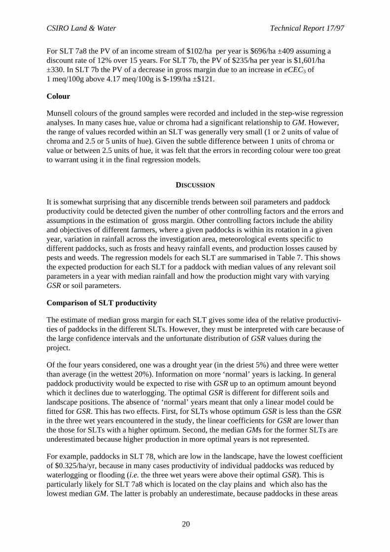
In the Transferral SLT (footslopes, 58% pasture), GM increased by $2.79/ha/yr ±2.46 for each1 ppm increase in available phosphorus in the 0-10 cm layer, AvP1 (range 11-54 ppm). Thepredicted GM with median AvP1 (25.5 ppm) and GSR is $135/ha/yr ±33.
In the Aeolian SLT (undulating plains with windblown clay, 44% pasture), GM increased by$225/ha/yr ±163 for each 1% increase in OC1 (range 0.9-1.9%) and by $24.7/ha/yr ±18.1 foreach 1 ppm increase in available phosphorus in the 20-30 cm layer, AvP3 (range 2.5-13.0ppm). The predicted GM with median OC1 (1.16%), AvP3 (6.6 ppm) and GSR is $222/ha/yr±72 in the Belfrayden soil-landscape unit (SLU) and $102/ha/yr ±62 in the East Bomen SLU.
The combined Alluvial and Gilgai SLTs could be divided into clay plains along the Murrum-bidgee and NW of The Rock (SLT 7a8, 63% pasture) and the lighter textured alluvium alongthe narrower valleys (SLT 7b, 75% pasture). In SLT 7b, GM decreased by $29.2/ha/yr ±17.8for each 1 meq/100g increase in effective cation exchange capacity of the 20-30 cm layer,eCEC3 (range 2.4-11.8 meq/100g). eCEC is the sum of exchangeable Al, Ca, Mg, Na and Kand is linked to clay content and type. Since most soils in this SLT have a sharp transitionfrom loam topsoil to clay subsoil, eCEC3 probably indicates sites where the transition to clayoccurs at shallower depths and which are more prone to waterlogging. Its effect on GM wasprobably exaggerated by the 3 wet years. The predicted GM for median eCEC3 (4.17meq/100g) and GSR is $235/ha/yr ±49. In SLT 7a8, no soil variables had any predictivecapability and predicted GM with median GSR is $102/ha/yr ±60. This is probably anunderestimate due to waterlogging in the wet years.
A method to ensure that the price being paid by a purchaser for a parcel of land is commensu-rate with its productive potential would have the following steps. The buyer decides on aninitial value for the land based on the median market price for land in the same SLT withmedian soil properties. Soil tests are used to determine whether important soil properties aregreater or less than the median for the SLT. The difference between measured and medianlevels of a soil property is used to estimate the difference in expected productivity, asmeasured by GM. The capitalised value of the difference in GM, estimated as the presentvalue (PV) of lost future production, is used to adjust the initial valuation. For example, in theErosional SLT, the PV of lost production due to each 1% rise in EAP1 above the median(5.23%) would be $-81/ha ±43 and that due to a 1% rise in OC1 above the median (1.32%)$790/ha ±693, assuming a commercial interest rate of 12% pa. over 15 years. Whilst thesesteps could be used explicitly to increase or decrease the maximum price the buyer is preparedto pay, they could also be used to improve financial planning by allowing for reductions inexpected income and the cost of remedial or preventative work.
Ensuring that land prices are commensurate with productive potential would increase thefinancial viability of farm enterprises. However, the scheme assumes the market price is basedon land in the SLT with median properties. It is not clear to what degree this is so and to whatextent market perception of different land types corresponds to the defined SLTs. Implemen-tation around Wagga Wagga would involve collecting data for years with more ‘normal’rainfall to improve the relationships discussed. Implementation on a wider scale wouldinvolve collecting a large quantity of soil and production data, which may not be feasible,especially since SLT maps are not available for many areas.

CSIRO Land & Water Technical Report 17/97
3
BACKGROUND
Land value and soil degradation
When land is purchased its market value depends on many factors of which only one is itsinherent productive potential. The productive potential depends on climate, location and soiltype. Within a given region, market value may take into account the climate and the differingproductivity of the various soil types but usually does so in an undefined and inconsistent way.Moreover, production is well below the potential in many areas of Australia. Whilst this ispartly caused by management factors, it is also caused by land degradation. If land is degraded(or improved) relative to the ‘norm’ for its type, there is currently no explicit way of adjustingthe market value.
Government agencies responsible for land management in Australia are concerned that thefailure of the market to set land values that reflect the degree of degradation (or improvement)reduces the incentive for land managers to prevent or ameliorate degradation. One way toencourage the market to increase the emphasis on degradation is to encourage financialinstitutions (who provide capital to support the market) to value land appropriately.
Finance industry perspective
The rural finance industry is concerned about the effects of unsustainable farming practices onland productivity and hence on the long-term health of the agriculture sector in which itinvests. Lowered productivity will, sooner or later, reduce the capital value of agriculturalland and the value of that land as security for loans to farm enterprises. Besides lowering thecapital value, lowered productivity also reduces profitability thereby decreasing the ability ofthe farm enterprise to service the loan and increasing the risk of default. This risk is exacer-bated by the fact that degraded land is often more susceptible to the extremes that are a featureof the Australian climate.
An important aspect of land quality is soil quality. Financial institutions may find it useful toknow the status of key soil parameters affecting productivity both when a loan is taken out atthe time of land purchase and during the term of the loan.
When setting up or reviewing a loan, the bank is interested in the profit/loss account and thebalance sheet. The profit/loss account indicates whether the enterprise has sufficient cash flowto service the loan; provide a reasonable family income and provide for on-going investmentin the farm. The balance sheet indicates whether the loan is stable. Financial institutions usefinancial indicators to assess the viability of the enterprise, but there is concern that these donot tell the whole story. For example, in one case study (pers. comm. C.K. Shearer, NAB) thefinancial indicators showed that farm viability was good. The return on capital was 5.7% andequity above 50%. The operating costs were rather high at 58% of income but were accept-able. However, much of the property was beginning to suffer from soil acidity and required aprogram of lime application for production to be maintained. This hidden cost of aboutA$28,000 would have a dramatic effect on cash flow, raising the operating cost ratio to 75%and lowering equity to less than 50%. These changes result in the farm appearing much lessviable. Such costs are ‘hidden’ from farm financial indicators unless revealed in advance byspecific soil measurements. This example shows the effect of land degradation on farmfinancial performance during the term of a loan. However, the effects would be similar if theland was being bought without prior knowledge of the soil acidity problem.

CSIRO Land & Water Technical Report 17/97
4
Rural bankers do not necessarily have training in the science of agriculture. They need asystem of benchmarks for various aspects of land quality and methods for making simplemeasurements (indicators) against these benchmarks that would allow them to factor landdegradation into farm finances. At the time of purchase, assessment would help ensure themaximum price bid for land is commensurate with its productive potential so that:
• The bank has adequate security against the loan;• The productive potential of the land is adequate to service the loan and provide income;• The farmer has allowed for any remedial work necessary for the land to achieve its
potential in the offer price.
During the term of a loan, assessments would help banks and farmers develop managementplans to prevent future degradation and ensure:
• Maintenance of the capital value of farm land both as a security for the bank and as anasset for future generations;
• Maintenance of the productive potential of the land which would decrease the likelihoodof defaulting on the loan and maintain farm profitability and farmer income;
• Avoidance of large, unplanned costs for remedial works which could severely affectcash flow and debt levels.
Such assessments clearly benefit both the bank and the farm enterprise. The only grouppotentially disadvantaged are farmers considering selling degraded land who could expect toreceive a lower price.
Land quality assessment
There are several approaches to assessment of land degradation. One approach is to assess thesustainability of the farming system. For example, the South Australian Department ofPrimary Industries uses a simple ‘Crop Rotation Sustainability Index’ to help farmers assesstheir land management practices. The index is calculated by scoring management practicesover a complete crop rotation or 10 years where there is no fixed rotation. Different crops/pastures score various points which are then averaged over the length of the rotation. Legumepastures score highest and cereals lowest. Similarly the various tillage and residue manage-ment options are scored and averaged. The sustainability index is then calculated as a numberbetween 0 and 10 from a combination of the average scores for crops, tillage and residuemanagement. Such schemes have the advantage of using readily available farm records and ofintegrating all aspects of management. However, the approach is intended as a quick andsimple management aid and not as an assessment of land value. It relies on a rather subjectiveand non-quantitative assessment of which land management practices are sustainable and theindex probably has an ill-defined relationship to productivity and capital value.
An alternative approach is to measure individual land properties including soil properties suchas pH, nutrient levels and structural condition. Assessment of these properties is moreobjective and quantitative. On the other hand, each measurement considers only one of manypossible factors affecting long-term productivity. Therefore it would be necessary to selectonly the most crucial properties for a given region or soil-landscape type. The degree to whichsuch factors relate to productivity and capital value is likely to vary. In the case of nutrientlevels and pH there is probably a relatively simple but noisy relationship but for soil structurethe relationship is likely to be much more complex.

CSIRO Land & Water Technical Report 17/97
5
AIMS
This was a pilot project to develop a methodology to determine which soil and land qualitiescan be measured/assessed at the farm level by rural advisory staff of the banking industry.
• To determine key land and soil properties/qualities that can assist determination of thevalue of land as a capital asset taking into account the impact of land degradation andsustainability of farming systems.
• To develop a set of preliminary indicators and rules for using measures and predictors toestimate changing capital value of land for the banking and rural finance industry.
At a workshop held at the start of the project in June 1995 to decide on a suitable approachthese aims were refined somewhat. In particular it was decided to concentrate on land in theWagga Wagga map sheet, since a soil-landscape survey of the sheet had recently beencompleted. The revised outcomes expected are:
• A set of recommended methods of testing for potential forms of soil degradation. Since thisis a pilot project this was limited to testing for:- soil acidity- phosphorus- waterlogging
• Methods for each of the tests above to convert the results into a capital value to besubtracted from/added to the market value. This should be based either on the cost of ame-lioration or on the value of lost returns.
• A land capability map (1:100,000) of the Wagga Wagga sheet showing areas where thesoils have:- similar potential productivity- similar potential limitations to production.
METHODS
The investigation was carried out in the region covered by the Wagga Wagga 1:100,000 Soil-Landscape map (Chen and McKane, 1997; McKane and Chen, 1997) in the NSW wheat-sheep belt and limited to soil properties that could be measured using disturbed soil samples.It had the following stages:
1. Selection of 80 paddocks within the Wagga Wagga map sheet from the major agriculturalsoil-landscape types (SLTs).
2. Soil sampling of the test paddocks followed by chemical analysis of the type available tofarmers. In order to allow the sampling of the largest possible number of paddocks, onlysoil parameters measurable using disturbed soil samples were considered. Hence no fieldmeasurements (e.g. of hydraulic properties) were made.
3. Estimation of paddock productivity from paddock histories compiled by interviewing thefarmer using gross margin as a measure of productivity.

CSIRO Land & Water Technical Report 17/97
6
4. Data analysis to determine:- average or median productivities for each group of SLTs- which of the measured soil properties relate to production for each SLT- benchmark values for each important soil attribute for each SLT- relationships between these soil properties and productivity within each SLT
5. Development of methods to translate differences between measured soil attribute valuesand the benchmark values for a given soil type into monetary value to be discounted fromor added to the land price. This monetary value should be based on either the value ofproduction lost due to degradation over a number of years or the capital cost of ameliora-tion.
6. Production of a land capability map of the Wagga Wagga area using the recently completed1:100,000 soil-landscape map which groups soil types that have similar potential produc-tivities and similar potential limitations to productivity.
Site selection
The Wagga Wagga 1:100,000 soil-landscape map divides the area into a number of soil-landscape units (SLU) on the basis of their topography, geology and soils. An SLU contains arange of associated soil types. The SLUs can be grouped into broad soil-landscape types(SLTs) as follows (Chen and McKane, 1997):1. Residual Landscapes (4.1% of map sheet) have deep soils formed by in situ weather-
ing, where the rate of soil formation is greater than that of ero-sion. Topography is elevated and level to undulating. Often lo-cated on summits, plateaux, terrace plains, peneplains and oldground surfaces. Stream channels are poorly defined.
2. Vestigial Landscapes (1.3%) have shallow soils formed by in situ weathering ofresistant parent materials. Topography is elevated and level toundulating. Includes summits, plateaux and old ground surfaces.
3. Colluvial Landscapes (10.4%) are affected by mass movement. Soil parent materialconsists of colluvial mass movement debris. Includes, cliffs,cliff-footslopes, scarps, landslides and talus.
4. Erosional Landscapes (22.5%) are affected by erosive action of running water and havewell defined streams. Soils are often shallow. Located on steepto undulating hillslopes.
5. Transferral Landscapes (14.3%) are deep deposits of parent materials eroded fromupslope. Streams are often discontinuous and slopes concave.Includes, footslopes, valley flats and fans.
6. Aeolian Landscapes (19.7%) have formed by accumulated deposition of wind-blownparticles, in this area mainly wind-blown clay known as parna.
7. Alluvial Soil Landscapes(25.1%) are formed by deposition along streams and rivers. Soilparent material is alluvium. Includes meander plains, backplains,levees, terraces and prior and current stream channels.
8. Gilgai Landscapes (1.7%) are clay plains with undulating microrelief associatedwith shrink-swell processes. Drainage patterns are usually dis-integrated.
9. Swamp Landscapes (0.9%) are permanently or seasonally waterlogged with wa-tertables close to the surface. Soil parent material includes largeamounts of decayed organic matter.

CSIRO Land & Water Technical Report 17/97
7
Residual, vestigial and swamp SLTs occupy only a small proportion of the map. The colluvialSLT occupies a significant area but little of it is used for agriculture because of its steep, rockytopography. Therefore, paddocks in these SLTs were not sampled.
80 paddocks from 37 properties were therefore selected mainly from within the erosional(SLT 4), transferral (SLT 5), aeolian (SLT 6), alluvial (SLT 7) and gilgai (SLT 8) SLTs. Forthe purposes of this project the gilgai SLT was included with the alluvial SLT because itoccupies a relatively small area within this map sheet and is similar to the alluvial SLT. It isreferred to as SLT 78. Paddock selection aimed to achieve approximately equal numbers ineach SLT and reasonable geographic coverage. The number of paddocks in each SLT isshown in Table 1.
In general two paddocks were sampled per property but this varied from one to four. Wherepossible paddocks within the same property were from different SLTs.
Soil sampling and analyses
Sampling was carried out over three weeks in the autumn of 1996. Before sampling eachpaddock was roughly mapped on the relevant 1:25,000 map sheet and measured using avehicle tachometer. Samples were taken along transects running downslope or parallel to thedirection of greatest change. Generally there were two transects per paddock spaced ¼ and ¾of the distance across the width of the paddock. In cases where there was a long, thin paddockwith the direction of greatest change running parallel to the shortest side, more transects wereused. Soil samples were taken at regular intervals along each transect. The interval betweensamples was equal to the greater of (transect length × no. transects/30) or 50m, giving amaximum of 30 sampling points per paddock. At each point the 0-10cm and 20-30cm soillayers were sampled using an auger. The samples from each layer were thoroughly mixed inthe field and sub-sampled for packing and transport.
The samples were sent to a commercial soil testing laboratory for routine analyses of the typereadily available to farmers for about $45. Soil parameters measured were:
AvP available phosphorus, ppm OC organic carbon, %AvK available potassium, ppm ExAl exchangeable aluminium, meq/100gAvS available sulphur, ppm ExCa exchangeable calcium, meq/100gpH in calcium chloride ExMg exchangeable magnesium, meq/100gEC electrical conductivity, dS/m ExNa exchangeable sodium, meq/100g
Table 1. Sampling with each SLT.
SLT No. paddocks No. properties from whichpaddocks were selected
1. Residual 1 14. Erosional 17 155. Transferral 22 176. Aeolian 14 117. Alluvial8. Gilgai
233
191
Total 80 37

CSIRO Land & Water Technical Report 17/97
8
Additional parameters calculated from these were:
ExK exchangeable K, meq/100g = 0.0022272 AvKeCEC effective cation exchange capacity, meq/100g = ExAl+ExCa+ExMg+ExK+ExNaEAP exchangeable aluminium percentage = ExAl / eCECECP exchangeable calcium percentage = ExCa / eCECEMP exchangeable magnesium percentage = ExMg / eCECEKP exchangeable potassium percentage = ExK / eCECESP exchangeable sodium percentage = ExNa / eCEC
In addition, the following parameters were measured in CSIRO laboratories:
Disp Emerson dispersion scoreHueD Munsell colour hue -dry HueM Munsell colour hue -moistValueD Munsell colour value -dry ValueM Munsell colour value -moistChromaD Munsell colour chroma -dry ChromaM Munsell colour chroma -moist
Emerson dispersion (Loveday, 1974) is measured by dropping small, air-dry aggregates intodistilled water and scoring the amount of dispersion after 2 and 20 hours. The maximum scoreof 16 indicates a highly dispersible soil. The average colour of each sample was measured bygrinding an air-dry sub-sample and comparing with standard Munsell colour charts to givehue, value and chroma under standard lighting conditions. Both dry and moist measures wererecorded.
Parameters for soil from the 0-10cm and 20-30cm depths are referred to using subscript 1 and3 respectively (e.g. pH1 and pH3).
Paddock productivity assessment
Standardised gross margin (GM, $/ha) was used to assess the relative productivities ofpaddocks under different management and being used for different enterprises. It is mostimportant that the method for estimating GM is understood so that the limitations of theresults are apparent. Standardised gross margin estimates a gross margin from paddock historyusing standard prices, machinery etc. and does not require any financial information from thefarmer. Farmers were interviewed by telephone to obtain the histories of the sampled pad-docks from 1992 to 1995. Farm records varied from excellent to non-existent. GM wascalculated as:
GM Livestock gross margin Cropincome Variable costs= + − Eqn. 1
An Excel 5 spread-sheet was developed to assist interviewing farmers (Appendix 1). One suchsheet was filled in for each paddock for each year.
Livestock gross margin
Estimating the income from livestock was undoubtedly the most difficult part of the grossmargin calculations. The chief problem was the lack of grazing records and in attributingproduction income and costs for a herd or flock to a particular paddock. The approach takenhad the following steps:

CSIRO Land & Water Technical Report 17/97
9
1. The enterprise was classified into one of five types - wethers, self-replacing ewes, second-cross lambs, cows and sucking calves, and steers.
2. The average stocking rate over the year for the paddock was estimated in several waysdepending on the preference of the farmer and the type of records kept (if any):• Stocking rate averaged for the whole year.• Herd/flock size, paddock area and the approximate period for which the paddock was
used based on actual knowledge or on the number and relative sizes of the paddocksthrough which the herd/flock was rotated.
• Herd/flock size, total area over which they were grazed (for a group of paddocks), theproportion of this area occupied by the paddock in question and the approximate pro-portion of the year for which the group of paddocks were used.
3. The average stocking rate in head/ha was converted to dry sheep equivalents (DSE)/ha.This was multiplied by the gross margin/DSE for the relevant enterprise, as shown in Ap-pendices 1 and 2, to give the livestock gross margin/ha for the paddock.
4. The cost of supplementary feed/ha was estimated from the feed usage (e.g. number ofbales/week × weight/bale or kg of grain/head and number of weeks of supplementaryfeeding) and the price of feed. Although most hay and grain used as feed was supplied fromwithin the property, it was costed at the market price shown in Appendix 1.
5. The livestock gross margin/ha from 3. was adjusted by subtracting the cost/ha of supple-mentary feed..
The gross margin/DSE for each enterprise type were from draft NSW Agriculture livestockbudgets. The sheep enterprises were based on a model flock of 1000 and the cattle ones on amodel herd size of 100. The gross margins included sales of wool, sheep and cattle togetherwith costs of animal management and selling for the model flock/herd. Some details for eachmodel are shown in Appendix 2. The gross margins did not include any pasture maintenanceor supplementary feed costs as these were estimated separately for each paddock-year.
There are clearly problems with this approach, including inaccuracies in estimating stockingrates and amounts of supplementary feed used. In addition, no allowance is made for differ-ences in livestock performance. For example, if a paddock was heavily overstocked, the grossmargin/DSE would generally be reduced. However, without better records and a lot moreinterviewing time, this approach appeared to be the only one practicable.
Crop income
Crop income was calculated as the yield obtained multiplied by the average farm-gate pricefor Wagga Wagga for 1992-1994 as quoted in The Land and shown in Appendix 1. The farm-gate price for canola was estimated as the capital city price less $25/t for delivery.
Income from hay or silage was calculated using hay prices in Wagga Wagga as quoted in TheLand, even when it was used within the property. In general, the yield of hay and silage hadnot been accurately recorded and had to be estimated from the approximate number ofbales/ha and the approximate weight/bale. Similarly, the quality and hence the price had to beestimated from the type and condition of the pasture. The value of silage was estimated to beequal to clover hay on a dry matter basis assuming dry matter contents of 85% for hay and

CSIRO Land & Water Technical Report 17/97
10
35% for silage (pers. comm. A. Kaiser, NSW Agriculture, Wagga Wagga). Hay prices haveonly been recorded by The Land since mid-1995. Therefore, the average prices for 1995/96were adjusted by the ABARE hay index to estimate prices for the remaining years. Theaverage of these four years was then used as the average for the period, as shown in Appendix1. The prices for subterranean clover and cocksfoot seed are estimates from local traders.
Variable costs
Variable costs were estimated from the operations and inputs recorded in the paddockhistories. Each operation was costed mainly using information from Wall (1996). Prices canbe found in the gross margin spread-sheet in Appendix 1.
Machinery costsMachinery costs for each cultivation, sowing, fertiliser or spraying operation were estimatedassuming standard hours/ha for each using a 82kW tractor and standard cost/hr for eachoperation from Wall (1996). The values can be found in Appendix 1.
Sowing costsActual sowing rates were used where possible. Where these had not been recorded or couldnot be estimated by the farmer, default values were used. Seed prices were obtained from Wall(1996) and are shown in Appendix 1.
Pasture establishment costs (cultivation and sowing) were attributed only to the year ofsowing. Where pasture was undersown with a cereal crop, the cost of the pasture seed wasincluded in the costs for the following year. In these cases the machinery costs for sowingwere attributed only to the cereal crop.
Fertiliser costsActual application rates of fertiliser were used together with the standard prices shown inAppendix 1, which were obtained from traders in the Wagga Wagga district. Where fertiliserwas applied with the seed, machinery costs were set to zero. Where fertiliser was broadcastseparately, the machinery costs were estimated as described above. ‘Machinery costs’ foraerial applications of fertiliser were costed at $14.00/ha.
Lime applications were recorded but not included in the gross margin calculations as theywere assumed to be capital improvements.
Irrigation costsSeveral paddocks were irrigated all or some of the years in question. This fact was recordedbut no cost was calculated due to the difficulty of estimating water use.
Herbicide and insecticide costsActual application rates of herbicides and insecticides were used together with the standardprices shown in Appendix 1, which were obtained from traders in the Wagga Wagga district.Where application rate was not known the manufacturers recommended rate was used.Machinery costs of spraying were estimated as described above. Where several chemicals hadbeen applied as a tank mix, machinery costs were only included for one chemical. ‘Machinerycosts’ for aerial applications of chemical were costed at $12.50/ha.

CSIRO Land & Water Technical Report 17/97
11
Harvest costsIt was assumed that contract harvesting was used. The total cost was estimated from the yieldand a standard harvest cost per tonne for each grain crop as shown in Appendix 1 (Wall,1996). An additional $25.00/ha for windrowing was included for canola crops. The harvestcosts of hay, silage and pasture seed were estimated as shown in Appendix 1.
Other costsOther costs included board and research levies and crop insurance as shown in Appendix 1.
Labour costsLabour costs were estimated from the total machinery hours ×1.25 and a labour cost of$12.50/hr.
Data analysis
Database
All soil data and a summary of the paddock history and gross margin data were incorporatedinto an Access 2® database. Any identifying information, including the paddock, property andfarmer names, the farmer’s address and the grid reference of the paddock is stored in aseparate database to maintain confidentiality.
The database contains 80 records relating to the dominant soil-landscape unit and type of eachpaddock; 160 records relating to the soil data for each paddock for each depth (0-10cm and20-30cm); and 320 records relating to the land use of each paddock in each year (1992, 1993,1994, 1995). The land use data is summarised as a land use code, total gross margin, livestockgross margin, crop and hay income and total variable costs. Also included are tillage, sowing,fertiliser, chemical, harvest and labour costs; inputs of N, P, S, lime and supplementary feed;stocking rates for each of the five enterprise types and crop/hay yields.
Rainfall data was included to account for the variability in production between years. Sincethis was not routinely available for each paddock, the data from Wagga Wagga airport (Table2) was applied to all paddocks for a given year. Growing season rainfall (GSR) was defined asthe rainfall between 1 April and 30 November.
Statistical analysis
Total gross margin was used as a measure of productivity for each paddock-year. The aimthen was to see how much of the variation in gross margins between could be accounted forby soil parameters measured in autumn 1996, allowing for variations in the rainfall of the
Table 2. Rainfall summary for Wagga Wagga for 1992-95 with long-term median (1948-94).
Year Total rainfall Growing season rainfall(1 April - 30 November)
Growing season rainfallPercentile
1992 921.2 mm 564.6 mm 88%1993 695.3 mm 515.9 mm 81%1994 475.0 mm 227.4 mm 5%1995 723.0 mm 590.6 mm 91%Median 574.8 mm 410.5 mm 50%

CSIRO Land & Water Technical Report 17/97
12
region. The main statistical tool used was linear regression analysis (using Excel 5® andGenstat 5®). Only linear models were used because the data did not justify the use of morecomplex models.
The only soil parameter adjusted to allow for possible changes during 1992-1996 was surfacepH in paddocks where lime had been applied. In this case the pH of the 0-10cm layer for theyears before lime application was adjusted as follows:
pH pre liming pHlime applied t / ha
1 1 19965 8
( ) ( )( )
.− = − Eqn. 2
This assumes a lime requirement of 4 t/ha to raise the pH by 1 unit in the 0-10cm layer wherebulk density is 1.0 t/m3. This requirement is adjusted to 5.8 t/ha to allow for a neutralisingvalue of the applied lime of 90% and an actual bulk density of 1.3 t/m3. This also assumes thatthe total pH increase occurred in the year of application.
It became apparent that the 8 paddock-years where irrigation was used would be difficult toincorporate in the analysis because there was no record of water use. 4 of these related to asingle paddock. Therefore irrigated paddock-years were excluded from the analysis. Similarly,the 7 paddock-years in which pasture seed (clover or cocksfoot) was grown generally hadmuch higher gross margins than other paddocks of a similar type. Because of this and thespecialised nature of pasture seed production, these paddock-years were also excluded.
There is no ideal way of analysing a large data set such as this with many possible explanatoryvariables, some of which are highly correlated. It was not made easier by the inherentvariability of the gross margin data due to the large variation between farmers and seasons anddue to errors in the paddock histories. Hence, soil parameters were only likely to account for asmall proportion of the variation in gross margin. Initial analysis involved step-wise regres-sion to find which soil variables showed most promise as explanatory variables (i.e. there is asignificant trend in gross margin as the variable changes). At the start a simple linear regres-sion model was fitted:
GM m X c= +1 1
where X is a soil or rainfall parameter, m1 the regression coefficient and c the intercept (thepredicted GM when X1 =0). Each parameter was tried as X1 in turn and those accounting forthe greatest proportion of the variance (r2) selected for further investigation. For the next step,one of these is chosen as X1 and an extra term is added to the equation:
GM m X m X c= + +2 2 1 1
Each unused parameter is then tried as X2 and those giving the greatest increase in r2 chosenfor further investigation. This can be repeated until adding extra terms results in negligibleincreases in r2. Clearly, there are very many different combinations that can be tried.
At each step it was also important to check the significance (P value) of each m coefficient.This is defined as the probability of obtaining by chance an m value as extreme the oneobtained. (I.e. the P values should be as low as possible, preferably less than 1%). It frequentlyhappened that adding a particular variable to the regression equation improved r2 but greatly

CSIRO Land & Water Technical Report 17/97
13
increased the P value of one of the previously fitted variables thereby making it redundant tothe regression model. This usually happened because the two variables were correlated.
In addition, it was necessary to check the data for outliers having a disproportionate andunrealistic effect on the fit.
Because a large number of potential regressors is considered, there is a danger that a variablemay be included in the model purely by chance. In any event several alternative models arelikely to fit almost equally well. Thus there is no single ‘correct’ model. The most suitablemust be chosen using statistical guidelines such as r2 and the P values of the coefficientstogether with knowledge of the likely effects of the soil parameters and what is realistic.
The data can also be analysed with the random variation separated into two components,between paddock variation and within paddock variation. Clearly soil properties would onlybe expected to explain between paddock variation, except where there is interaction withrainfall. Where this was done it gave similar results to the analyses reported here. In particu-lar, estimates of effects were largely unchanged, but there was some change to estimates ofstandard errors. However, this form of analysis should be considered in future analyses of dataof this type.
RESULTS
Paddock productivity is controlled by many factors other than soil and regional rainfall. Hencethe proportion of variation accounted for by soil parameters and rainfall (r2) was generallysmall. Despite this and the inaccuracies and assumptions in the estimation of gross margin, itwas possible to find statistically significant relationships and to develop regression models topredict gross margin from soil parameters and rainfall. These are discussed below.
Although the models may be highly significant, both overall (F probability) and with respectto each coefficient (t probability), the standard errors and confidence intervals are large,because the proportion of variance accounted for (r2 or r2adjusted) is small. In discussingpossible regression models below, care has been taken to quote the 95% confidence intervals,(E-CI95%, E+CI95%, where CI95% is generally equal to about 2× the standard error) for esti-mated regression coefficients and GM predictions. The only way to reduce the 95% confi-dence intervals is to increase the sample size. When considering the results below it is mostimportant to take note of the confidence intervals quoted.
Results for all soil-landscape types
After excluding irrigated paddock-years and those growing pasture seed, there were 305paddock-years remaining. Not surprisingly, GSR was the variable accounting for the mostvariation, with an r2 of 12.7%. The variables most effective when added to the regressionmodel as a second term were (with r2) EMP1 (16.6%), ExMg1 (15.4%), ExMg3 (15.4%), ECP1
(15.2%), eCEC3 (15.2%), ExNa3 (14.9%), ExNa1 (14.8%) and ExCa3 (14.7%). All of theseexcept ECP1 are highly correlated with high values being associated with the clay soils alongthe Murrumbidgee floodplain and the clay plains to the west of The Rock. Whilst it waspossible to add statistically significant third and even fourth terms to the model with GSR andEMP1, interpretation of the resulting models was difficult. The relationship between GM andthe additional variables was often quite different for different soil-landscape types or sub-

CSIRO Land & Water Technical Report 17/97
14
types, but the strength of the relationship for a particular type or sub-type dominated theoverall regression and gave a significant coefficient that would be quite misleading whenapplied to the other types or sub-types. Therefore it seemed more appropriate to investigateeach SLT separately.
Erosional Soil Landscapes (SLT 4)
There were 17 paddocks within SLT 4 giving 68 paddock-years. Two paddock-years wereexcluded from further analysis because subterranean clover was grown for seed in 1992 and1993 in one of the paddocks. 4 paddocks were in the Lloyd (ld) SLU; 8 in the Pulletop (pu)SLU and 5 in the Yarragundry (ya) SLU. Lloyd and Pulletop are on metasediments withslopes of 10-20% and 3-10%, respectively, and local relief of 30-60 m and 15-40 m, respec-tively. Yarragundry is on granite with slopes of 8-20% and local relief of 30-80 m.
Livestock was the only land use in 59% of the 68 paddock-years (Table 10). Of the remainingpaddock-years, 22% were used for cropping, 7.5% for cropping and livestock (either as splitpaddocks, cereal crops with some grazing of vegetative growth or failed crops which weregrazed instead of harvested), and 7.5% for hay and livestock. Lime was applied to 4 paddocksduring 1992-1995.
GSR as a single variable accounted for 11.5% of the variation. The variables accounting forthe most variance when added as a second variable with GSR were EC1, ExNa1, ESP1, ExNa3,ESP3, eCEC1, ExCa1, ECP1, ExAl1, EAP1 and pH1.
The actual values of variables relating to soil salinity or sodicity (EC1, ExNa1, ESP1, ExNa3,ESP3) were generally very low and the regression result was greatly influenced by twopaddocks with moderate EC1 (0.1 dS/m), ESP1 (3%) and ESP3 (5%), which produced positiveregression coefficients. The accumulation of salt (albeit slight) at these sites probablyindicates they are wetter than the others and produce better in dry years. In fact, in the 1994drought, these paddocks had GMs of $430/ha and $285/ha, whereas the other paddocks inSLT 4 all produced less than $175/ha with a mean of $70/ha. This does not mean that salinityor sodicity is not important in this SLU, merely that this data set does not contain enoughinformation to determine whether it is or not.
A combination of GSR, eCEC1 and OC3 accounted for 37% of the variance. Subsoil organiccarbon was negatively correlated with GM (i.e. had a negative coefficient). Values weregenerally low around 0.35% and near the detection limit. Higher values were associated withpoorer producing paddocks under permanent pasture. Thus, in this case, it appeared thatsubsoil organic carbon was a consequence of low productivity rather having an influence on it.
Parameters related to soil acidity showed the most promise as explanatory variables. pH1,ExAl1, EAP1 and ExCa1 accounted for 17.2%, 18.8%, 22.3% and 29.2% of the variancerespectively, when combined with GSR. No other suitable parameters could be added to amodel with pH1 or ExCa1 without the P value of one of the regression coefficients becomingnon-significant. ExAl1 and EAP1 could both be combined with OC1 to give r2 of 25.6% and28.2% respectively. The model chosen as being most informative was:
GM GSR EAP OC= − + − +74 0 0 427 119 1161 1. . . Eqn. 3

CSIRO Land & Water Technical Report 17/97
15
where GM is in $/ha, GSR in mm and both EAP1 and OC1 in percent. Details of the regressioncoefficients and the analysis of variance are shown in Table 3. There were no significantinteractions between EAP1 or OC1 and the SLUs within the erosional SLT.
By substituting the median values for GSR (410.5 mm, 1948-1994), EAP1 (5.23%) and OC1
(1.32%) Eqn. 3 can be expressed as:
( ) ( )GM EAP OC= − − + −19190 119 5 23 116 1321 1. . . . Eqn. 4
This implies that in a ‘normal’ year the median paddock in SLT 4 could be expected toproduce $192/ha ±45. This will be referred to as the estimated median GM. This could beexpected to decrease by $11.90/ha ±6.30 for each 1% EAP1 is above its median and toincrease by $116.00/ha ±101.80 for each 1% OC1 is above its median. The median is usedsince it is more robust that the mean which can be influenced by extreme values especiallywhen the number of samples is small.
The present value (PV) of an income stream of $192/ha per year is $1,307/ha ±306 assuming adiscount rate of 12% over 15 years. An interest rate of 12% corresponds to the commerciallending rate. A discount period of 15 years was chosen because the term of a loan for agricul-tural land would normally be between 10 and 20 years. The PV of the reduction in grossmargin due to each 1% increase in EAP1 above the median is $-81/ha ±43. Similarly the PV ofthe increase due to each 1% increase in OC1 above the median is $790/ha ±693.
Transferral Soil Landscapes (SLT 5)
There were 22 paddocks within SLT 5 giving 88 paddock-years. 12 paddocks were in theBecks Lane (bk) SLU; 8 in the Vincent Road (vi) SLU and 1 each in the Benloch (bl) andRedbank (rb) SLUs. Becks Lane is on the footslopes of metasedimentary hills with slopes of2-4% and local relief of 5-15 m. Vincents Road is on the footslopes of hills of Devoniansandstone with slopes <3% and local relief <10 m. Benloch is eroded piedmont inclined frommetasedimentary ranges with slopes of 3-6% and local relief of 10-20 m, whilst Redbank is onpiedmont slopes with slopes <3% and local relief <10 m.
In 58% of paddock-years livestock was the only land use (Table 11). Of the remainingpaddock-years, 31% were used for cropping, 7% for cropping and livestock, 3.5% fallow and1% each for hay, hay and cropping and hay and livestock. Lime was applied to 2 paddocksduring 1992-1995.
Table 3. Summary of regression analysis for SLT 4.
Variable Coefficient Standard error 95% confidencelimits
t probability
constant -74.0 92.9 ±187 0.429GSR 0.427 0.136 ±0.271 0.003EAP1 -11.9 3.15 ±6.30 <0.001OC1 116 50.9 ±101.8 0.026r2 0.283r2
adjusted 0.248F probability <0.001 (from analysis of variance)degrees of freedom 62

CSIRO Land & Water Technical Report 17/97
16
GSR as a single variable accounted for 13.1% of the variation. The variables accounting forthe most variance when added as a second variable with GSR were AvP1 and AvK1 which hadr2 of 18.0% and 17.6%, respectively. However, no further parameters could be added to theregression model without the P value of one of the regression coefficients becoming non-significant. For available P, the model is:
GM GSR AvP= − + +90 0 0 375 2 79 1. . . Eqn. 5.
where GM is in $/ha, GSR in mm and AvP1 in ppm. Details of the regression coefficients andthe analysis of variance are shown in Table 4. There was no significant interaction betweenAvP1 and the SLUs within the SLT 5.
By substituting the median values for GSR (410.5 mm) and AvP1 (25.5 ppm) Eqn. 5 can beexpressed as:
( )GM AvP= + −13517 2 79 25 51. . . Eqn. 6
This implies that in a ‘normal’ year the median paddock in SLT 5 could be expected toproduce $135/ha ±33. This could be expected to increase by $2.79/ha ±2.46 for each 1 ppmAvP1 is above its median.
The PV of an income stream of $135/ha per year is $921/ha ±223 assuming a discount rate of12% over 15 years. The PV of the reduction in gross margin due to each 1 ppm decrease inAvP1 below the median is $-19/ha ±17.
Aeolian Soil Landscapes (SLT 6)
There were 14 paddocks within SLT 6 giving 56 paddock-years. One paddock-year wasexcluded from further analysis because subterranean clover was grown for seed in 1992. 6paddocks were in the Belfrayden (be) SLU and 8 in the East Bomen (eb) SLU. Belfraydenconsists of moderately deep (80-120 cm) soils formed on a gently undulating plain of thickalluvium with additions of parna. Slopes are about 1% and local relief <5 m. East Bomenconsists of shallow to moderately deep (40-150 cm) soils on undulating rises of granodioritewith slopes of 3-10% and local relief of 15-40 m.
Table 4. Summary of regression analysis for SLT 5.
Variable Coefficient Standard error 95% confidencelimits
Probability
constant -90.0 61.4 ±122 0.146GSR 0.375 0.102 ±0.202 <0.001AvP1 2.79 1.24 ±2.46 0.026r2 0.180r2
adjusted 0.161F probability <0.001 (from analysis of variance)degrees of freedom 85

CSIRO Land & Water Technical Report 17/97
17
44.5% of paddock-years were used for cropping only, 30.4% for livestock only, 12.5% for hayand livestock, 8.9% for cropping and livestock and 1.8% each for hay and cropping (Table12). One paddock was limed during 1992-1995.
GSR as a single variable accounted for 29.0% of the variation. The variables accounting forthe most variance when added as a second variable with GSR were (with r2) AvK1 (37.2%),ExAl3 (37.2%), Disp1 (36.9%), SLU factor (be or eb) (34.5%) and OC1 (33.9%). Values forExAl3 were low and near the limit of detection. The regression was highly influenced by twooutliers with higher values. The range of values for Disp1 was small and less than those thatwould be considered likely to affect soil structure and plant growth. ExAl3 and Disp1 were notinvestigated further.
Of the remaining variables, two groups of potential models become apparent, when addingthird or fourth terms. In the first, GSR and AvK1 are the first two variables and in the second,GSR and OC1. AvK1 and OC1 cannot be included in the same model because they are highlycorrelated and one of them becomes redundant.
The group of models using GSR and AvK1 itself divides into three sub-groups depending onwhether the SLU factor, eCEC3 or ExCa3/ECP3 is used as the third term. These variables donot combine well for the same reason as above. The most common variable useful as a fourthterm with any of the three sub-groups is ExMg3/EMP3. These models achieved r2 of >48%.
For the group of models using GSR and OC1, the SLU factor or ECP3 could be used as thirdvariables. ExCa1, AvP3 or EKP1 could be combined with SLU as fourth variables but onlyEKP1 could be combined with ECP3. All achieved r2 of >45%.
The variations in AvK1 are probably important as a reflection of clay mineralogy and content,rather than the soil’s nutritional status. Therefore, OC1 was chosen as more suitable than AvK1
because it can be influenced by land management. There was also a significant interactionbetween SLU and GSR (i.e. the coefficient for GSR was different for the two SLUs). The mostuseful model appeared to be:
GMGSR SLU be
GSR SLU ebOC AvP=
− + =
− + =
+ +665 113
521 0 485225 24 71 3
.
.. Eqn. 7
Table 5. Summary of regression analysis for SLT 6.
Variable Coefficient Standard error 95% confidencelimits
Probability
SLU=be -665 154 ±309 <0.001SLU=eb -521 156 ±313 0.002GSR•SLU=be 1.13 0.210 ±0.422 <0.001GSR•SLU=eb 0.485 0.181 ±0.364 0.010OC1 225 81.0 ±163 0.008AvP3 24.7 8.99 ±18.1 0.008r2 0.529r2
adjusted 0.481F probability <0.001 (from analysis of variance)degrees of freedom 49

CSIRO Land & Water Technical Report 17/97
18
where GM is in $/ha, GSR in mm, OC1 in percent and AvP3 in ppm. Which of the terms insquare brackets is used depends on the whether the SLU is be or eb. (‘|’ means ‘given that’).Details of the regression coefficients and the analysis of variance are shown in Table 5. Therewas no significant interaction between OC1 or AvP3 and the SLUs within SLT 6.
By substituting the median values for GSR (410.5 mm), OC1 (1.16%) and AvP3 (6.6 ppm)Eqn. 7 can be expressed as:
( ) ( )GMSLU be
SLU ebOC AvP=
=
=
+ − + −222
102225 116 24 7 6 61 3. . . Eqn. 8
This implies that in a ‘normal’ year the median paddock in SLT 6 in the Belfrayden (be) SLUcould be expected to produce $222/ha ±72 and that in the East Bomen (eb) SLU $102/ha ±62.Production could be expected to increase by $225/ha ±163 for each 1% OC1 is above itsmedian and by $24.7/ha ±18.1 for each 1 ppm AvP3 is above its median.
For the Belfrayden SLU, the PV of an income stream of $222/ha per year is $1,510/ha ±487assuming a discount rate of 12% over 15 years. For the East Bomen SLU, the PV of $102/haper year is $696/ha ±420.The PV of a decrease in gross margin due to a decline of 1% in OC1
below 1.16% is $-1,534/ha ±$1,109. That due to each 1 ppm decline in AvP3 below 6.6 ppm is$-168/ha ±123.
Alluvial and Gilgai Soil Landscapes (SLT 78)
There were 26 paddocks within SLT 78 giving 104 paddock-years. 4 paddock-years wereexcluded from further analysis because subterranean clover seed was grown in one paddock in1993 and 1994 and cocksfoot seed in another paddock in 1992 and 1993. Another 8 paddockyears were excluded because they were irrigated: one paddock in all four years; one in 1993and 1994; and two in 1994 only. Of the 25 included paddocks, 3 were in the BullenbongPlains (bu) SLU, 4 in Grubben (gb), 2 in Kurrajong Plain (kp), 6 in Mangoplah (ma), 1 inBullenbong Road (br) and 9 in O'Briens Creek (ob). Bullenbong Plains occurs on the exten-sive alluvial plains of lower Burkes Creek with slopes <1% and local relief <1 m. Grubben isvery gently undulating alluvial plains with slopes of 1-2% and local relief <5 m. KurrajongPlains is the extensive level plain of higher Murrumbidgee floodplain with slopes <1% andlocal relief <2 m. Mangoplah and Bullenbong Road are extensive alluvial plains mainly alongBurkes Creek with slopes <1% and local relief <10 m. O’Briens Creek is gently undulatingalluvial plains with slopes <3% and local relief <10 m.
53.8% of paddock-years were used for livestock only, 17.3% for crops only, 6.7% for hay andlivestock, 4.8% for cropping and livestock or cropping, livestock and hay, 2.9% for hay andcropping, 1.9% for hay alone and 1% fallow (Table 13). Two paddocks were limed during1992-1995.
GSR as a single variable accounted for only 6.4% of the variation. Many parameters accountedfor more, in particular EMP1, eCEC3, ExCa3, and ExMg3 which all had r2 over 15%. However,no other variables could be added as third terms without one of the terms becoming non-significant. All these variables, in particular EMP1 were closely correlated with SLU. Pad-docks in Bullenbong Plains (bu), Grubben (gb) and Kurrajong Plains (kp) SLUs all had EMP1
> 25% and those in Bullenbong Road (br), Mangoplah (ma) and O’Briens Creek (ob) SLUs all

CSIRO Land & Water Technical Report 17/97
19
had EMP1 < 25%. The former group all occur on clay alluvium along the Murrumbidgeefloodplain or on the extensive clay plains to the NW of The Rock. The latter group occur oncoarser textured alluvium in the narrower floodplains along the creeks in the SE of the mapsheet. Therefore SLT 78 was divided into two sub-types: SLT 7a8, containing the clay plains(bu, gb and kp SLUs), and SLT 7b, containing the coarser textured flood plains. When thesesub-types were included as a factor they accounted for 10.2% of the variation. If GSR and SLTwere included in a regression model, other variables could only be added if interactions withSLT were taken into account. The most significant included subsoil eCEC.
GM GSReCEC SLT a
eCEC SLT b= +
− =
− =
0 32559 5 20 7 8
223 29 2 7
3
3
..
.Eqn. 9
where GM is in $/ha, GSR in mm and eCEC3 in meq/100g. In this case there was an interac-tion between eCEC3 and the soil-landscape sub-type, which appears in the square brackets(i.e. the constant and regression coefficient are different for the two sub-types. Details of theregression coefficients and the analysis of variance are shown in Table 6.
By substituting the median values for GSR (410.5 mm) and eCEC for SLT 7a8(17.35 meq/100g) and SLT 7b (4.17 meq/100g) Eqn. 9 can be expressed as:
( )( )
( )( )
GMeCEC SLT a
eCEC SLT b
eCEC SLT a
eCEC SLT b
= +− − − =
− − =
=− − =
− − =
133312 5 20 17 35 7 8
101 7 2917 417 7
102 5 20 17 35 7 8
235 2917 417 7
3
3
3
3
. . .
. . .
. .
. .
Eqn. 10
This implies that in a ‘normal’ year the median paddock in SLT 7a8 could be expected toproduce $102/ha ±60. Production could be expected to decrease by $5.20/ha ±8.13 for each1 meq/100g eCEC3 is above its median. Alternatively, eCEC3 could be ignored for SLT 7a8since the coefficient is not significant. The expected production for the median paddock inSLT 7b in a ‘normal’ year is $235/ha ±49, which would be reduced by $29.17/ha ±17.75 foreach 1 meq/100g eCEC3 is above its median.
Table 6. Summary of regression analysis for SLT 78.
Variable Coefficient Standard error 95% confidencelimits
Probability
GSR 0.325 0.122 ±0.242 0.009SLT=7a8 59 102 ±203 0.564SLT=7b 223 76.7 ±152 0.005eCEC3•SLT=7a8 -5.20 4.09 ±8.13 0.208eCEC3•SLT=7b -29.2 8.93 ±17.7 0.002r2 0.268r2
adjusted 0.235F probability <0.001 (from analysis of variance)degrees of freedom 87
CSIRO Land & Water Technical Report 17/97
20
For SLT 7a8 the PV of an income stream of $102/ha per year is $696/ha ±409 assuming adiscount rate of 12% over 15 years. For SLT 7b, the PV of $235/ha per year is $1,601/ha±330. In SLT 7b the PV of a decrease in gross margin due to an increase in eCEC3 of1 meq/100g above 4.17 meq/100g is $-199/ha ±$121.
Colour
Munsell colours of the ground samples were recorded and included in the step-wise regressionanalyses. In many cases hue, value or chroma had a significant relationship to GM. However,the range of values recorded within an SLT was generally very small (1 or 2 units of value ofchroma and 2.5 or 5 units of hue). Given the subtle difference between 1 units of chroma orvalue or between 2.5 units of hue, it was felt that the errors in recording colour were too greatto warrant using it in the final regression models.
DISCUSSION
It is somewhat surprising that any discernible trends between soil parameters and paddockproductivity could be detected given the number of other controlling factors and the errors andassumptions in the estimation of gross margin. Other controlling factors include the abilityand objectives of different farmers, where a given paddocks is within its rotation in a givenyear, variation in rainfall across the investigation area, meteorological events specific todifferent paddocks, such as frosts and heavy rainfall events, and production losses caused bypests and weeds. The regression models for each SLT are summarised in Table 7. This showsthe expected production for each SLT for a paddock with median values of any relevant soilparameters in a year with median rainfall and how the production might vary with varyingGSR or soil parameters.
Comparison of SLT productivity
The estimate of median gross margin for each SLT gives some idea of the relative productivi-ties of paddocks in the different SLTs. However, they must be interpreted with care because ofthe large confidence intervals and the unfortunate distribution of GSR values during theproject.
Of the four years considered, one was a drought year (in the driest 5%) and three were wetterthan average (in the wettest 20%). Information on more ‘normal’ years is lacking. In generalpaddock productivity would be expected to rise with GSR up to an optimum amount beyondwhich it declines due to waterlogging. The optimal GSR is different for different soils andlandscape positions. The absence of ‘normal’ years meant that only a linear model could befitted for GSR. This has two effects. First, for SLTs whose optimum GSR is less than the GSRin the three wet years encountered in the study, the linear coefficients for GSR are lower thanthe those for SLTs with a higher optimum. Second, the median GMs for the former SLTs areunderestimated because higher production in more optimal years is not represented.
For example, paddocks in SLT 78, which are low in the landscape, have the lowest coefficientof $0.325/ha/yr, because in many cases productivity of individual paddocks was reduced bywaterlogging or flooding (i.e. the three wet years were above their optimal GSR). This isparticularly likely for SLT 7a8 which is located on the clay plains and which also has thelowest median GM. The latter is probably an underestimate, because paddocks in these areas

CSIRO Land & Water Technical Report 17/97
21
are capable of producing high yielding crops as shown by the high levels of crop inputsapplied by some farmers. For other SLTs, in particular SLT 6, it is likely that the three wetyears did not reach their optimal GSR.
Clearly, information on production in more normal years would improve understanding of theway paddocks in each SLT respond to rainfall. Such information might allow determination ofthe optimal GSR for each SLT and the shape of the response curve to GSR. Assuming theshape is not linear, the median predicted GM would then have to be calculated differently. Itwould be necessary to predict GM for a paddock with median soil properties for each year inthe rainfall record. Median GM is then the median of all the predicted values and would give atruer picture of the relative productivities of the different SLTs.
Differences in the land use between SLTs also has an affect on their median GMs and GSRcoefficients. Table 8 shows there is a trend for the median GM to increase as the proportion ofcropped paddock-years decreases, with the exception of SLT 6-be. There are two possiblereasons for this rather surprising result. First, the method of estimating GM for livestockenterprises may be overestimating GM relative to crops. Second, cropped paddocks were morelikely to be adversely affected by waterlogging in the wetter than average years. This would beless so for the well drained, red-brown earths found in the Belfrayden (be) SLU of SLT 6 thanin the other SLTs. It is also noticeable that the GM confidence intervals relative to median GMare high for SLTs 6-eb and 7a8 (around 0.6) compared to the other SLTs (0.20-0.32). Thiscould be evidence that in wetter than average years crop damage occurs sporadically in timeand space leading to greater variability in GM in these SLTs. In SLT 7a8 waterlogging wouldbe the main cause of crop damage in wet years, as discussed above. However, the cause ofdamage in SLT 6-eb and 5 is less obvious. SLT 5 often lies at the break of slope wherewaterlogging can occur in wet years. SLT 6-eb is located on long piedmont slopes wherewaterlogging would not be expected to occur. It is possible that structure decline has occurredon these slopes where they are intensively cultivated and that this leads to crusting andhardsetting in wet years. Further evidence is the sheet erosion that can occur on these slopes
Table 7. Summary of regression models for each SLT quoted at the median growing season rainfall (410.5mm)and the median values of each of the soil parameters included. The intervals quoted are the 95% confi-dence intervals.
SLT r 2adjusted Median GM
$/ha/yrGM adjustment terms ($/ha/yr)
due to variations in:
Soil parameters GSR
4. Erosional 24.8% 192 ± 45 -11.9 ± 6.3×(EAP1-5.23)
+116 ± 102×(OC1-1.32)
+0.427 ±0.271×(GSR-410.5)
5. Transferral 16.1% 135 ± 33 +2.79 ± 2.46×(AvP1-25.5)
+0.375 ±0.202×(GSR-410.5)
6. Aeolian- SLU be
- SLU eb48.1%
222 ± 72
102 ± 62
+225 ± 163×(OC1-1.16)
+24.7 ± 18.1×(AvP3-6.6)
+1.13 ±0.422×(GSR-410.5)
+0.485 ±0.364×(GSR-410.5)
78. Alluvial/gilgai - 7a8
- 7b23.5%
102 ± 60
235 ± 49
-
-29.2 ± 17.8×(eCEC3-4.17)
+0.325 ±0.242×(GSR-410.5)

CSIRO Land & Water Technical Report 17/97
22
(Chen and McKane, 1997) and that SLT 6-be is twice as responsive to GSR ($1.13/ha/mm) asSLT 6-eb ($0.485/ha/mm) (Table 7).
Overall, it is important not to put too much emphasis on the relative productivities of theSLTs found in this study, unless gross margin estimates for more normal years can be addedto the data set.
Effect of soil properties on productivity
The low r2 in the regression analyses show that individual soil properties are only some ofmany factors controlling paddock productivity. However, within an SLT, there are significanttrends in production with specific soil properties. Fig. 1 shows the distribution of various soilparameters in paddocks in each SLT.
Soil acidity and aluminium
Fig. 1 shows that soil acidity is a problem in a significant proportion of paddocks in mostSLTs. One of the main effects of low pH is to increase the amount of available aluminium inthe soil, which is toxic to many plant species. There is a strong relationship between pH andexchangeable aluminium percentage in the surface soil (Fig. 3), with EAP increasing with pHsless than 4.8. The surface soil of 79% of the 80 paddocks sampled had pHs less than 4.8 (and28% of sub-surface soils). It is interesting to note that lime was applied to only 9 of the 80paddocks during 1992-1995 and that the average amount applied was only 2.0 t/ha. Clearly,farmers are failing to implement adequate liming strategies, either because they are notreceiving and/or understanding information about its importance or because they are finan-cially unable to.
Despite the generally low pHs encountered in this study and the well established importanceof pH in the region, pH1 or EAP1 only appeared as explanatory variables in SLT 4 (erosional).This is probably because of the ranges of EAP1 encountered. In SLT 6-be, 6-eb and 7a8, therewere no EAP1 values above 10% and the minimum pH1 is about 4.4. Given the variation inGM and number of other factors affecting it, it is unlikely that the influence of EAP would beapparent without some more extreme values. In SLTs 5 and 7b there are many paddocks withhigh EAP1, but no response to EAP1 or pH1 was detected. Production was presumably limitedby factors other than EAP, such as waterlogging. In SLT 5, 65% of paddocks had EAP1 >10%and the paucity of low EAP1 values may also have contributed to the lack of a response.
Table 8. Land use summary for each soil-landscape type or sub-type excluding irrigated paddocks and thosegrowing pasture seed. ‘Crop’ includes paddock-years classified in Tables 10-13 as ‘Crop’,‘Crop+Livestock’ and ‘Crop+Hay’. ‘Pasture’ includes ‘Livestock’, ‘Livestock+Hay’ and ‘Hay’.
SLT Crop Fallow Pasture Estimatedmedian GM,
$/ha/yr
6-be 70% 0% 30% 222 ± 726-eb 47% 0% 53% 102 ± 625 39% 3% 58% 135 ± 337a8 37% 0% 63% 102 ± 604 30% 2% 68% 192 ± 457b 23% 2% 75% 235 ± 49

CSIRO Land & Water Technical Report 17/97
23
0%
25%
50%
75%
100%
0 40 80
Available P (0-10 cm depth), ppm
Per
cent
less
than
SLT 4
SLT 5
SLT 6-be
SLT 6-eb
SLT 7a8
SLT7b0%
25%
50%
75%
100%
5 10 15
Available P (20-30 cm depth), ppm
Per
cent
less
than
0%
25%
50%
75%
100%
0.5% 1.0% 1.5% 2.0% 2.5%
Organic C (0-10 cm depth)
Per
cent
less
than
0%
25%
50%
75%
100%
0 10 20
eCEC (20-30 cm depth), meq/100g
Per
cent
less
than
0%
25%
50%
75%
100%
0% 10% 20%
Exch. Al percent (0-10 cm depth)
Per
cent
less
than
0%
25%
50%
75%
100%
4.0 4.5 5.0 5.5pH (in CaCl2) (0-10 cm depth)
Per
cent
less
than
Fig. 1. Cumulative frequencies of soil parameters in paddocks within various SLTs.

CSIRO Land & Water Technical Report 17/97
24
-300
-200
-100
0
100
200
300
0% 5% 10% 15% 20% 25% 30% 35%
Exchangeable aluminium percent, 0-10cm
Pre
dict
ed G
M, $
/ha
Fig. 2. Influence of EAP1 on predicted GM in SLT 4 assuming median rainfall and median OC1 (1.32%). Thepoints show predictions at the 0, 25, 50, 75 and 100 percentiles of EAP1. The dotted lines show the95% confidence limits.
0%
5%
10%
15%
20%
25%
30%
35%
4.0 4.2 4.4 4.6 4.8 5.0 5.2 5.4 5.6 5.8pH (in CaCl2)
Exc
h. A
l per
cent
4
5
6-be
6-eb
7a8
7b
0-10 cm depth
Fig. 3. Relationship between exchangeable aluminium percentage and pH in surface soils of the samplepaddocks. The line represents:
( )Ln. .
. . .
. .
e ..
EAPpH
pH pH
EAPpH
pHpH
1
1
1 1
1
1
3 5621
4 602 5 0
13 21 3 562 5 0
0 0100 5 0
543732 5 01
=− ≥
− <
=≥
<
−
Eqn. 11
where EAP1 is expressed as a proportion (NOT a percent).
SLT 4 has a wide range of EAP1 values and is less likely to have been affected by waterlog-ging because of its steeper slopes. The effect of EAP1 on predicted GM is shown in Fig. 2.

CSIRO Land & Water Technical Report 17/97
25
However, it is likely that acidity and EAP have an effect on GM in other SLTs, in particularSLTs 5 and 7b. To determine the magnitude of the effect it would be necessary to samplemore paddocks in these SLTs that have higher pHs and lower EAP1 and to add data for yearswith more normal rainfall when waterlogging is unlikely to be a limiting factor.
Organic carbon
Organic carbon is a significant predictor of productivity in SLTs 4 and 6. The relationshipbetween OC1 and predicted GM is shown in Fig. 4. Organic carbon content is closely linked to
-100
0
100
200
300
400
500
0.8% 1.0% 1.2% 1.4% 1.6% 1.8% 2.0% 2.2% 2.4% 2.6% 2.8%
Organic Carbon, 0-10cm
Pre
dict
ed G
M, $
/ha
SLT 4
SLT 6-be
SLT 6-eb
Fig. 4. Influence of OC1 on predicted GM in SLTs 4, 6-be and 6-eb assuming median rainfall. For SLT 4 thepredictions assume median EAP1 (5.23%) and for SLTs 6-be and 6-eb, median AvP3 (6.6 ppm). Thepoints show predictions at the 0, 25, 50, 75 and 100 percentiles of OC1. The dotted lines show the 95%confidence limits.
0.5%
1.0%
1.5%
2.0%
2.5%
3.0%
0 2 4 6 8 10 12 14 16Mean tillage costs 1992-1995, $/ha/yr
Org
anic
car
bon,
0-1
0cm
4
6-be
6-eb
Fig. 5. Influence of mean tillage costs over 1992-1995 on OC1 in SLTs 4, 6-be and 6-eb. The line is the linearregression equation: OC Mean tillage costs1 155 0 0472= −. . where OC1 is in percent. The re-
gression has r2=0.245 and an F probability of 0.46%.
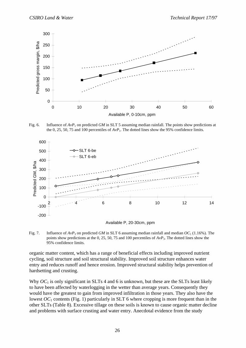
CSIRO Land & Water Technical Report 17/97
26
organic matter content, which has a range of beneficial effects including improved nutrientcycling, soil structure and soil structural stability. Improved soil structure enhances waterentry and reduces runoff and hence erosion. Improved structural stability helps prevention ofhardsetting and crusting.
Why OC1 is only significant in SLTs 4 and 6 is unknown, but these are the SLTs least likelyto have been affected by waterlogging in the wetter than average years. Consequently theywould have the greatest to gain from improved infiltration in those years. They also have thelowest OC1 contents (Fig. 1) particularly in SLT 6 where cropping is more frequent than in theother SLTs (Table 8). Excessive tillage on these soils is known to cause organic matter declineand problems with surface crusting and water entry. Anecdotal evidence from the study
0
50
100
150
200
250
300
0 10 20 30 40 50 60
Available P, 0-10cm, ppm
Pre
dict
ed g
ross
mar
gin,
$/h
a
Fig. 6. Influence of AvP1 on predicted GM in SLT 5 assuming median rainfall. The points show predictions atthe 0, 25, 50, 75 and 100 percentiles of AvP1. The dotted lines show the 95% confidence limits.
-200
-100
0
100
200
300
400
500
600
2 4 6 8 10 12 14
Available P, 20-30cm, ppm
Pre
dict
ed G
M, $
/ha
SLT 6-be
SLT 6-eb
Fig. 7. Influence of AvP3 on predicted GM in SLT 6 assuming median rainfall and median OC1 (1.16%). Thepoints show predictions at the 0, 25, 50, 75 and 100 percentiles of AvP3. The dotted lines show the95% confidence limits.

CSIRO Land & Water Technical Report 17/97
27
supports this, with paddocks in the East Bomen SLU showing signs of rilling when the farmerwas using many tillage passes. In fact, for SLTs 4 and 6, OC1 can be predicted to some extentfrom the average cost of tillage over the period from 1992 to 1995 as shown in Fig. 5.
That SLT 6 is more responsive to OC1 than SLT 4 is probably because of the greater croppingfrequency in SLT 6 and consequently the potential for higher GMs.
Available phosphorus
Although phosphorus, as a major nutrient, could be expected to have an impact on paddockproductivity, AvP1 only appears as significant in SLT 5 (Fig. 6). However, P levels in theSLTs where cropping is important (5, 6 and 7a8) are generally adequate in the surface soil(57%, 73% and 81%, respectively, of paddocks with AvP1 >25 ppm) except in SLT 5. Sub-surface P, AvP3, only becomes important in SLT 6 (Fig. 7) which has both a high proportionof cropping and high yields in the wetter years. This points to the importance of subsoilfertility in areas of high production.
Effective cation exchange capacity
Within the alluvial SLT (78), there is a significant relationship between productivity and sub-surface cation exchange capacity, eCEC3, in sub-type 7b (the coarser textured alluvium alongthe narrower creek floodplains) (Fig. 8). The relationship for sub-type 7a8 (the heavy texturedclay plains) is not significant. eCEC is closely related to clay content since the bulk of theexchange complex is located on the clay surface, especially in subsoils where organic matter(another contributor to eCEC) is low. Since most soils in this SLT are duplex, eCEC3
probably indicates shallower depths to the clay B horizon. As discussed earlier, productivitymay have been adversely affected by waterlogging in many paddocks of this SLT in the wetterthan average years. This regression relationship provides additional evidence for this, sincesoils with clay B horizons nearer the surface would be more prone to waterlogging. Whetherthis relationship would hold if information on more normal years was included is not known.
-150
-100
-50
0
50
100
150
200
250
300
350
0 5 10 15 20 25 30
Effective cation exchange capacity, 20-30cm, meq/100g
Pre
dict
ed G
M, $
/ha
SLT 7a8
SLT 7b
Fig. 8. Influence of eCEC3 on predicted GM in SLT 78 assuming median rainfall. The points show predic-tions at the 0, 25, 50, 75 and 100 percentiles of eCEC3. The dotted lines show the 95% confidencelimits. As can be seen from the confidence limits, the relationship for SLT 7a8 is not significant.
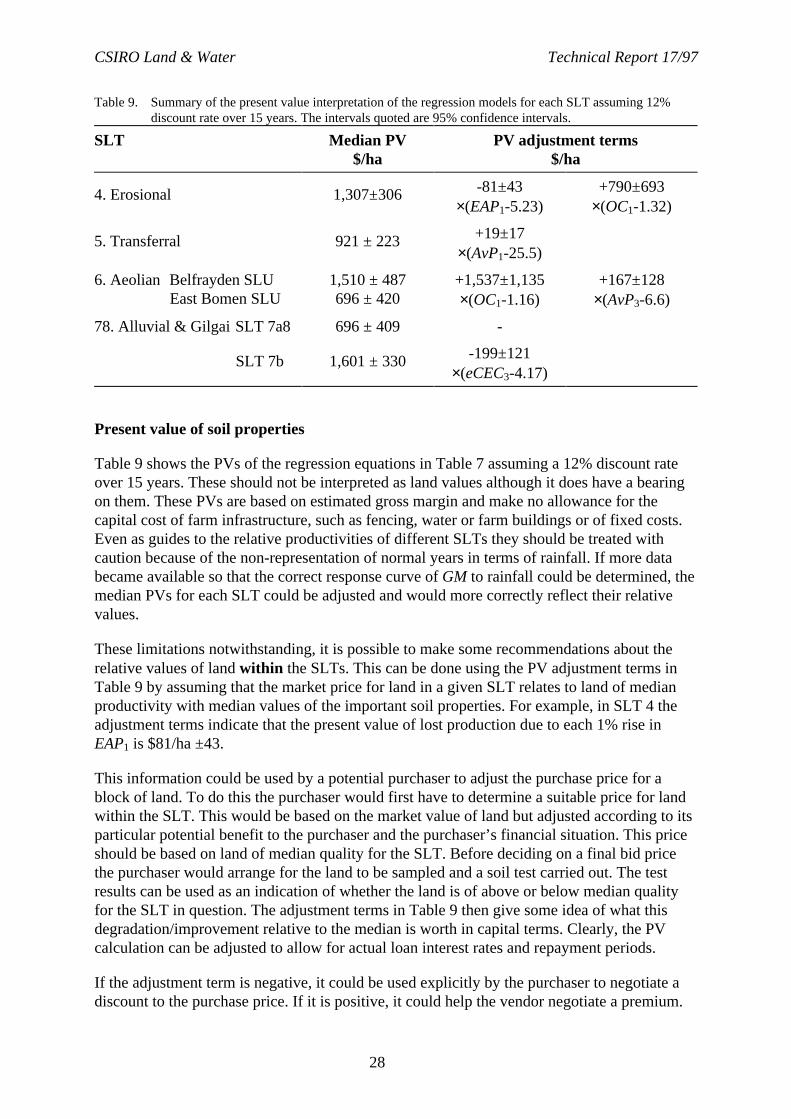
CSIRO Land & Water Technical Report 17/97
28
Present value of soil properties
Table 9 shows the PVs of the regression equations in Table 7 assuming a 12% discount rateover 15 years. These should not be interpreted as land values although it does have a bearingon them. These PVs are based on estimated gross margin and make no allowance for thecapital cost of farm infrastructure, such as fencing, water or farm buildings or of fixed costs.Even as guides to the relative productivities of different SLTs they should be treated withcaution because of the non-representation of normal years in terms of rainfall. If more databecame available so that the correct response curve of GM to rainfall could be determined, themedian PVs for each SLT could be adjusted and would more correctly reflect their relativevalues.
These limitations notwithstanding, it is possible to make some recommendations about therelative values of land within the SLTs. This can be done using the PV adjustment terms inTable 9 by assuming that the market price for land in a given SLT relates to land of medianproductivity with median values of the important soil properties. For example, in SLT 4 theadjustment terms indicate that the present value of lost production due to each 1% rise inEAP1 is $81/ha ±43.
This information could be used by a potential purchaser to adjust the purchase price for ablock of land. To do this the purchaser would first have to determine a suitable price for landwithin the SLT. This would be based on the market value of land but adjusted according to itsparticular potential benefit to the purchaser and the purchaser’s financial situation. This priceshould be based on land of median quality for the SLT. Before deciding on a final bid pricethe purchaser would arrange for the land to be sampled and a soil test carried out. The testresults can be used as an indication of whether the land is of above or below median qualityfor the SLT in question. The adjustment terms in Table 9 then give some idea of what thisdegradation/improvement relative to the median is worth in capital terms. Clearly, the PVcalculation can be adjusted to allow for actual loan interest rates and repayment periods.
If the adjustment term is negative, it could be used explicitly by the purchaser to negotiate adiscount to the purchase price. If it is positive, it could help the vendor negotiate a premium.
Table 9. Summary of the present value interpretation of the regression models for each SLT assuming 12%discount rate over 15 years. The intervals quoted are 95% confidence intervals.
SLT Median PV$/ha
PV adjustment terms$/ha
4. Erosional 1,307±306 -81±43×(EAP1-5.23)
+790±693×(OC1-1.32)
5. Transferral 921 ± 223 +19±17×(AvP1-25.5)
6. Aeolian Belfrayden SLUEast Bomen SLU
1,510 ± 487696 ± 420
+1,537±1,135×(OC1-1.16)
+167±128×(AvP3-6.6)
78. Alluvial & Gilgai SLT 7a8
SLT 7b
696 ± 409
1,601 ± 330
-
-199±121×(eCEC3-4.17)

CSIRO Land & Water Technical Report 17/97
29
Alternatively, the adjustment term could be used to give the purchaser a greater awareness ofthe likely productivity of the land relative to other land of a similar type. This would enablemore realistic planning of the income that could be expected from the land and aid determina-tion of a purchase price commensurate with its earning potential.
There are several problems with the system proposed above. First, it assumes market value iscurrently based on SLT, but does not take into account individual soil characteristics such asexchangeable aluminium or organic carbon. In reality, the market takes soil-landscapeinformation into account in a rather undefined way that probably does not correspond to themapped SLTs. For example, within SLT 4, there are some elevated, steep paddocks whosemarket price would currently be considered well below other paddocks in the SLT on the basisof their limited potential for pasture improvement. However, if the market value was adjustedas proposed above, the value could be artificially low. Effectively, the land would have beendiscounted twice, once in a rather undefined way by the market and once according to a soilproperty.
Second, in SLTs where most land is degraded relative to what might be considered desirablefor a particular soil property, this system gives no indication that the land is degraded. Forexample, in SLT 5 93% of sampled paddocks had pHs below 4.8 and, as discussed earlier, thismay be a part of the reason why neither pH nor exchangeable aluminium could be used topredict GM. In valuing the SLT, the market may or may not take into account its generallylower productivity due to soil acidity, (and may or may not recognise acidity as the cause). Ifthe lower productivity has been factored into the value, then the land will not be overvaluedrelative to its productive potential. However, one of the aims of the system is to encourage soilimprovement by reflecting such improvements in the capital value of the land. In such SLTs,improvements to pH by liming would not result in a gain in value in this system becauseneither pH nor exchangeable aluminium appear as adjustment terms. Clearly in SLTs wheremost of the land is known to be degraded, there is a need to include paddocks which havebeen ameliorated, so that the benefits to production accruing from amelioration can bedetermined.
One solution to the latter problem, is to set an optimum level for a given soil property and todiscount the land value by the cost of restoring the property to its optimum level. This is onlyfeasible for soil properties that can be altered directly, such as pH, which can be adjusted byapplying lime. For properties such as organic carbon, it is difficult to calculate the cost ofimprovement, because they depend more on sustained conservative soil management overmany years. Other soil properties such as clay content and effective cation exchange capacitycannot be readily altered by management, so the only way of adjusting land value is on thebasis of lost production.
Discounting land value on the basis of the cost of restoration is also problematic because themarket price may relate to land in a sub-optimal condition where most land in a givencategory is already degraded. In such situations should the discount be the cost of restoring thesoil property to its median level or to its optimum level?
The effect of the different ways of adjusting land value can be investigated through thefollowing scenarios for SLT 4. In these scenarios, the net present value (NPV) of variousstrategies is investigated relative to the NPV of buying land in SLT 4 of median EAP1 (5.23%≡ pH1 of 4.54) and OC1 (1.32%) and assuming that this land produces an income stream of$192/ha/yr. In all the scenarios OC1 is held constant at the median value for the SLT. The

CSIRO Land & Water Technical Report 17/97
30
change in GM as EAP1 changes follows Eqn. 4. The relationship between EAP1 and pH1 isassumed to be that given in Eqn. 11 and shown in Fig. 3. The lime required to increase the pHof the 0-10 cm layer by 1 unit is assumed to be 5.8 t/ha and the cost of lime (applied) $62/t.The interest rate is assumed to be 12% and the borrowing period 15 years. Rainfall is assumedto be equal to the median each year. The following scenarios can then be investigated withtheir relative NPVs being shown in Fig. 9. Note that for scenarios where discounts are applied,the discount will be negative (i.e. a premium) when pHs are greater than 4.54.
1. The purchaser pays the market price for land in SLT 4 with no adjustments. In this scenariothe relative NPV would be negative if EAP1 was above the median (and pH1 was belowmedian). This results from annual income being lower than $192 and having a lower PV asshown in Table 9. If EAP1 was equal to the 75th percentile (8.3% ≡ pH1 of 4.41), the rela-tive NPV would be $-249/ha.
2. The purchaser discounts the market price by the PV of lost production due to higher EAP1
levels. In this case, the discount at the time of purchase ($-249/ha for the 75%ile EAP1)compensates for lower income so that the relative NPV is zero.
3. The purchaser discounts the market price by the cost of lime required to bring the pH to alevel corresponding to the median EAP1, but does not apply lime. The discount is notsufficient to negate the effect of lower income. At the 75%ile for EAP1 (pH 4.41), the pHdifference is 0.13 units, which would require 0.75 t/ha lime costing $46/ha. However, thisconsiderably lower than the PV of lost production ($-249/ha) and gives a relative NPV of$-202/ha
4. The purchaser pays the market price with no adjustments (as 1) but applies lime to raisethe pH to 4.8 and lower EAP1 to 2.04%. (The costs of maintaining it at 4.8 are not in-cluded). The cost of lime is outweighed by the gain in production resulting in a positiverelative NPV. At the 75%ile for EAP1, this would require 2.27 t/ha lime, costing $141/ha,to raise the pH by 0.39 units. The increased income has a PV of $507/ha giving a relativeNPV of $117/ha (=-249+507-141).
-1000
-800
-600
-400
-200
0
200
400
600
800
1000
4.2 4.3 4.4 4.5 4.6 4.7 4.8
pH, 0-10 cm
Rel
ativ
e N
PV
, $/h
a
1
2
3
4
5
6
pH ≡ median EAP1
pH ≡ 75th percentile EAP1
Fig. 9. The net present value relative to land with median EAP1 and OC1 of various scenarios discussed in thetext for SLT 4.

CSIRO Land & Water Technical Report 17/97
31
5. The purchaser discounts the market price by the PV of lost production due to higher EAP1
levels (as in 2) and then applies lime to raise the pH to 4.8 (as in 4). This scenario pro-duces the greatest NPVs for the purchaser because, as for 4, the increase in income out-weighs the cost of the lime, but, in this case, is added to a zero relative NPV resulting fromthe application of a discount as in scenario 2. At the 75%ile for EAP1, the discount for lostproduction relative to the median would be $249/ha. 2.27 t/ha of lime would be requiredcosting $141/ha to raise the pH by 0.39 units. The increased income has a PV of $507/hagiving a relative NPV of $366/ha (=-249+507-141+249).
6. The purchaser discounts the market price by the cost of lime required to bring the pH to alevel corresponding to the median EAP1 (as in 3) but applies lime to raise the pH to 4.8 (asin 4). This scenario produces a constant relative NPV of $164/ha. At the 75%ile for EAP1,the discount for the cost of lime to raise pH to the median would be $46/ha. The cost of thelime actually applied to raise pH to 4.8 would be $141/ha. The increased income has a PVof $507/ha giving a relative NPV of $164/ha (=-249+507-141+46).
The range of outcomes from the scenarios presented suggest that there is some flexibility inhow the problem of accounting for soil degradation at the time of land purchase is tackled.Clearly a purchaser of land in SLT 4 with a lower than normal pH will benefit from theknowledge gained from testing the soil prior to purchase. The pH would suggest that liming isalways a sensible option even if the purchase price was not discounted. However, planningthis at the time of purchase would enable the extra cost of liming to be built into the borrow-ing requirement. Of course, if the purchase price can be reduced, the benefit of liming will begreater. It is interesting to note that discounts based on the PV of lost production are greaterthan those based on rectifying the problem.
For soil properties that cannot be so easily adjusted, only scenarios 1 and 2 are possible, withany discounts being based on the PV of lost production. Since the magnitude of these can bequite large, it would make sense for land managers to maintain land in reasonable conditionrelative to these parameters, since purchasers could demand a large discount if a system suchas the one proposed here was adopted.
RECOMMENDATIONS
If financial institutions wish to ensure that a potential borrower buying agricultural land ispaying a realistic price they should take into account the ‘capital value’ of particular soilproperties. Bearing in mind that this was a pilot project carried out only in the Wagga Waggaregion and the limitations of the data set, the steps envisaged would be as follows:
• The soil-landscape map is used to determine the soil landscape type or sub-type (SLT) ofthe block of land about to be purchased. Those investigated for the Wagga Wagga mapsheet include:SLT 4 ErosionalSLT 5 TransferralSLT 6-be The Belfrayden soil-landscape unit (SLU) of the aeolian SLTSLT 6-eb The East Bomen SLU of the aeolian SLTSLT 7a8 The clay plain SLUs of the alluvial and gilgai SLTs which includes the Bullen-
bong Plains (bu), Grubben (gb) and Kurrajong Plains (kp) SLUs and probablythe Farnham (fa) SLU, although the latter was not sampled.

CSIRO Land & Water Technical Report 17/97
32
SLT 7b The coarser textured SLUs of the alluvial SLT, which includes the BullenbongRoad (br), Mangoplah (ma) and O’Briens Creek (ob) SLUs and probably theBig Springs (bs) SLU, although the latter was not sampled.
The Residual, Vestigial, Colluvial and Swamp SLTs and the Currawarna (ca) and Pearson(pe) SLUs of the aeolian SLT were not investigated.
• The SLT of the land can be used to check that the planned income is realistic. The figuressuggested are gross margins for a year of median rainfall and assume land with medianlevels for the important soil properties (see below). These figures must be treated withextreme caution at this stage due to the non-representation in the data set of ‘normal’ yearsin terms of rainfall. The range given refers to the 95% confidence interval.SLT 4 $192/ha/yr ± 45SLT 5 $135/ha/yr ± 33SLT 6-be $222/ha/yr ± 72SLT 6-eb $102/ha/yr ± 62SLT 7a8 $102/ha/yr ± 60SLT 7b $235/ha/yr ± 49
• Bulked soil samples are taken from 0-10 cm depth for all paddocks except those in SLT7a8. In addition, samples at 20-30 cm are taken for paddocks in SLTs 6 and 7b. The sam-ples are analysed by a commercial soil testing laboratory.
• The differences between the measured soil properties and the median for the SLT are usedto adjust the expected median gross margin. The adjustment terms are (in $/ha/yr):
SLT 4 ( ) ( )[ ] ( ) ( )[ ]− ± ⋅ − + + ± ⋅ −119 6 3 5 23 116 102 1321 1. . . .EAP OC
SLT 5 ( ) ( )+ ± ⋅ −2 79 2 46 25 51. . .AvP
SLT 6 ( ) ( )[ ] ( ) ( )[ ]+ ± ⋅ − + + ± ⋅ −225 163 116 24 7 181 6 61 3OC AvP. . . .
SLT 7b ( ) ( )− ± ⋅ −29 2 17 8 4173. . .eCEC
where EAP is the exchangeable aluminium percent (of eCEC); OC the organic carboncontent (%); AvP available phosphorus (ppm) and eCEC the effective cation exchangecapacity (meq/100g) calculated as the sum of exchangeable cations (Al, Ca, Mg, Na andK). Parameters with subscript 1 refer to the 0-10 cm layer and those with subscript 3 to the20-30 cm layer. 95% confidence intervals are shown for each coefficient. Negative valuesare subtracted from the median gross margin and positive ones added to it.
• The capital value of the adjustment terms is calculated as the present value (PV) of lost (orgained) future income due to the difference between actual and median soil properties forthe SLT. For an interest rate of 12% (the commercial lending rate) over 15 years the ad-justment terms translate to (in $/ha):
SLT 4 ( ) ( )[ ] ( ) ( )[ ]− ± ⋅ − + + ± ⋅ −81 43 5 23 790 693 1321 1EAP OC. .
SLT 5 ( ) ( )+ ± ⋅ −19 17 25 51AvP .
SLT 6 ( ) ( )[ ] ( ) ( )[ ]+ ± ⋅ − + + ± ⋅ −1 537 1135 116 167 128 6 61 3, , . .OC AvP
SLT 7b ( ) ( )− ± ⋅ −199 121 4173eCEC .
These figures can be regarded as the increase or decrease in the land value due to thedifference between the measured level of a soil property and the median for the SLT.
CSIRO Land & Water Technical Report 17/97
33
• The information can be taken into account when deciding on a purchase price for the land.For example it could be used to lower or raise the maximum bid price for the land. Alter-natively it can assist financial planning for the farm by taking into account any reduction inexpected income and the cost of any remedial or preventative work necessary.
• During the term of an existing loan the financial institution could request that the soilproperties be regularly monitored. This would enable planning, both physically and finan-cially, for remedial or preventative work to maintain the soil properties at certain levels sothat the capital value of the asset held as security is maintained. This would also help farm-ers maintain the long-term productivity of their land and reduce the risk of decreased prof-itability, increased debt and default.
INDUSTRY IMPLICATIONS
This project has tried to find a means of estimating the capital value of soil properties as theyaffect agricultural production in farmers’ paddocks. This is directed towards helping landmanagers include soil as part of the capital assets of an agricultural enterprise. Adoption ofsuch a scheme would increase the degree to which land prices reflect land degradation andprovide extra incentive for land managers to adopt conservative soil management practices.
It should be stressed that adoption does not necessarily require that the PV discounts orpremiums resulting from a particular soil property are used literally. Rather they can be usedto bring soil factors into the overall assessment of land value.
The direct effect of this scheme would be to help farmers pay more realistic prices for land.This would ensure greater financial viability for the farmer because the price paid is commen-surate with its earning potential. For soil properties that can be directly adjusted, such as pH, itwould allow financial planning for the cost of amelioration of degraded land to take placebefore purchase, so that such costs do not upset farm finances at a later date. Similarly, regularmonitoring of relevant soil properties, would enable planning for amelioration or changes inmanagement practice to take place before degradation starts affecting production.
Improvements in financial planning by farm enterprises also benefit the financial institutionsthat are financing them. First it lowers the risk of farm finances getting into difficulties andultimately the risk of default. Second, it ensures that the value of the land held as securityagainst a loan is both realistic to start with and is maintained during the course of the loan.
It is unclear how much of this information is already factored into the ‘market’ price of aparticular piece of land. Certainly, there are allowances for soil-landscape type, but the degreeto which these correspond to the formally defined SLTs is not known. For this scheme towork it would be necessary for the market to set a value for the SLT but not to take anyinformation about individual soil properties into account, whether explicitly or implicitly. Forexample land that ‘looks’ less productive may be devalued by the market, without knowledgethat it is a soil property reducing its productivity. If a discount were applied due to a particularsoil property, the final price may have effectively been discounted twice. It is also unclear howmuch the market takes into account lowered productivity in situations where most of a givenSLT is degraded and where it is therefore difficult to detect a production response to the soilproperty. In these situations, the market price may or may not reflect the degraded nature ofthe land. Nevertheless, it is important to know how the land would respond to improvement,

CSIRO Land & Water Technical Report 17/97
34
so that the value of such improvements can be factored in to the price and provide incentive tomake such improvements.
If such a scheme was successfully implemented, changes in soil properties could occur in thelong-term as land managers adopt more conservative practices. Whilst this would be adesirable outcome, it would cause problems with the scheme. As more land in a given SLTwas improved with respect to a particular soil property, the median value of that propertywould change. The ‘market’ might then perceive ‘normal’ land in this SLT as correspondingto the new median and change its price accordingly. Since the scheme uses the median valuesto decide whether the land should be valued above or below the market price, it would benecessary to update the medians used in the adjustment terms.
CONCLUSIONS
It is possible to detect the effects of soil properties on paddock productivity in the uncon-trolled reality of farmers’ paddocks despite the many other factors affecting productivity.Moreover it has been shown that the level of a soil property measured at a given point in timehas some relation to productivity over the previous four years. It is possible to give some ideaof the change in income that could be expected as various soil properties change. If soils weretested before purchase, the trends found could be used by land purchasers to assist financialplanning with respect to future income, borrowing requirements and the cost of soil ameliora-tion strategies. Indeed, they could be used by land managers to improve financial planning forland they already own.
One option is to use the trends to negotiate a discount/premium on the purchase price so thatthe price paid better reflects the earning potential of the land. This could be on the basis of thePV of lost future production. In some cases where a soil property can be easily altered, thediscount/premium could be on the basis of the cost of restoring the soil property to its medianlevel.
The soil properties that are important vary between different soil-landscapes types. In theerosional SLT (4) the exchangeable aluminium percent (EAP1) and organic carbon content(OC1) of the surface soil were important. In the transferral SLT (5) available phosphorus ofthe surface soil (AvP1) was the only soil property with predictive value. OC1 and sub-surfaceavailable phosphorus (AvP3) had predictive value in the aeolian SLT (6). The alluvial andgilgai SLTs (7 and 8) were considered together, but then divided into to groups. SLT 7a8consisted of the heavy clay plains where no soil parameters had predictive value. SLT 7bconsisted of the coarser textured alluvium along the narrower valleys, in which sub-surfaceeffective cation exchange capacity (eCEC3) could be used to predict productivity. eCEC3 wasprobably acting as a surrogate for clay content and indicating soils more prone to waterlogging.
In all of this it must be remembered that this is a pilot project and there are limitations to theconclusions drawn.• It must be emphasised that the confidence limits on the trends found are very large.• The unusual range of growing season rainfall during the years incorporated in the study
(one year <5th percentile, 3 >80th percentile), means that:

CSIRO Land & Water Technical Report 17/97
35
- The response of production to rainfall measured in each SLT may be incorrect leading toan incorrect estimate of median production. In particular, median production may be un-derestimated in those SLTs whose optimum rainfall is less than that in the 3 wet years.
- Some important trends may have been omitted and others amplified. For example, inSLT 7b the response to eCEC3 may have been amplified because of the three wetter thanaverage years. Conversely, in SLT 5, a response to pH or EAP was not found, possiblybecause waterlogging had a greater limiting effect.
• Production responses to some important soil properties may have been masked in someSLTs because such a high proportion of the paddocks sampled were degraded that a re-sponse could not be detected. For example, the lack of a reponse to pH or EAP in SLT 5(see above) may also have been because almost all the paddocks were acid.
The results could be improved by the inclusion of production data for years with rainfallcloser to the median (i.e. between the 5th and 80th percentiles). This information wouldimprove confidence in both the GM responses to various soil properties within various SLTsand in the relative GMs of different SLTs. In addition, inclusion of non-acid paddocks in thoseSLTs which appeared predominantly acid, would help to establish the GM response to acidity.Whilst the market price for land in these SLTs may already reflect their predominantly acidcondition, information on the response would allow land managers to determine the likelyfinancial benefit of liming.
Additional work still to be carried out on the data set is to estimate growing season rainfall foreach paddock using ESOCLIM (Hutchinson, 1989) and to include landscape factors such asslope and aspect. It would also be useful to compare the results with actual land values.
Implementation of this system even in the Wagga Wagga region would require more data.This would ensure adequate representation of ‘normal’ years in terms of rainfall. More datawould enable detection of production responses to particular soil properties that are currentlymasked in some SLTs. It is also necessary to include indicators of soil hydraulic behaviour,which were omitted from this study due to time constraints.
Implementation in other regions, especially those with different farming systems and differentclimates, would clearly require a large amount of additional data and may not be possible inareas where soil-landscapes have not been mapped.
REFERENCES
Chen, X.Y. and McKane, D. 1997. ‘Soil Landscapes of the Wagga Wagga 1:100 000 Sheet.’Report. Department of Land and Water Conservation, Sydney.
Hutchinson, M.F. 1989. A new method for spatial interpolation of meteorological variablesfrom irregular networks applied to the estimation of monthly mean solar radiation, tem-perature, precipitation and windrun. CSIRO Division of Water Resources TechnicalMemorandum 89/5.
Loveday, J. 1974. Aggregate stability. In: ‘Methods for Analysis or Irrigated Soils’ (Ed. J.Loveday), pp.75-77. Commonwealth Bureau of Soils Technical Communication 54, Com-monwealth Agricultural Bureaux, Farnham Royal, UK.
McKane, D. and Chen, X.Y. 1997. ‘Soil Landscapes of the Wagga Wagga 1:100 000 Sheet.’Map. Department of Land and Water Conservation, Sydney.
Wall, L. 1996. Winter Crop Budgets. Southern Zone 1996. NSW Agriculture.

CSIRO Land & Water Technical Report 17/97
36
APPENDIX 1GROSS MARGIN SPREADSHEET
Site No. YearProperty Paddock size, haDescription
LimeTotal
GROSS MARGIN $ /ha
GROSS MARGIN - LIVESTOCKTotal $ /ha
Proportion No head Area DSE Stocking GM/DSE GM/haof year (1) rate (1)
ha DSE/head DSE/ha $/DSE $/haSheep -wethers (1) $ 15.14 $ /ha $ /ha
ha 1 $ 15.14 $ /ha $ /haSheep - self replacing ewes (1) $ 16.53 $ /ha $ /ha
ha 2.1 $ 16.53 $ /ha $ /haSheep - 2nd cross lambs (1) $ 16.26 $ /ha $ /ha
ha 2.3 $ 16.26 $ /ha $ /haCattle - Cows and calves (1) $ 20.23 $ /ha $ /ha
ha 16.4 $ 20.23 $ /ha $ /haCattle - Steers 200-400kg (1) $ 25.63 $ /ha $ /ha
ha 9 $ 25.63 $ /ha $ /ha
Supplementary feed Occurrence Rate/ha $/unit $/ha Hay (3) t/ha $ /t $ /ha $- /ha Silage t/ha $ 45.42 /t $ /ha $- /ha Grain (oats) kg/ha $0.14 /kg $ /ha $- /ha
INCOME - CROPSTotal $ /ha
Occurrence GrainCrop Yield Price
t/ha $/t
Wheat t/ha $ 162.67/t $ /haTriticale t/ha $ 159.56/t $ /haBarley - feed (2) t/ha $ 159.99/t $ /haOats - grain t/ha $ 137.82/t $ /haLupins t/ha $ 197.06/t $ /haCanola t/ha $ 327.76/t $ /haLucerne pastureSub. clover pasturePhalaris based pastureHay (3) t/ha $ /t $ /haOther (3) $ /ha

CSIRO Land & Water Technical Report 17/97
37
VARIABLE COSTS - CROPSTotal $ /ha
No. times Machinery Inputscarried out hrs/ha $/hr $/ha Rate/ha $/unit $/ha
Burn 0.1 hr/ha
Cultivation Chisel plough (119 kW tractor) 0.38 hr/ha $22.44/hr $ 8.53/ha $ /ha Disc plough (82 kW tractor) 0.38 hr/ha $15.03/hr $ 5.71/ha $ /ha Scarify (82 kW tractor) 0.38 hr/ha $14.52/hr $ 5.52/ha $ /ha Wideline (82 kW tractor) 0.16 hr/ha $16.19/hr $ 2.59/ha $ /ha Harrow (82 kW tractor) 0.34 hr/ha $14.59/hr $ 4.96/ha $ /ha
Sowing Set to $0.00/ha if undersown inprevious year
Wheat 0.31 hr/ha $22.48/hr $ 6.97/ha kg/ha $0.45 /kg $ /ha $ /ha Triticale 0.31 hr/ha $22.48/hr $ 6.97/ha kg/ha $0.50 /kg $ /ha $ /ha Barley 0.31 hr/ha $22.48/hr $ 6.97/ha kg/ha $0.40 /kg $ /ha $ /ha Oats 0.31 hr/ha $22.48/hr $ 6.97/ha kg/ha $0.50 /kg $ /ha $ /ha Lupins 0.31 hr/ha $22.48/hr $ 6.97/ha kg/ha $0.50 /kg $ /ha $ /ha Field peas 0.31 hr/ha $22.48/hr $ 6.97/ha kg/ha $0.50 /kg $ /ha $ /ha Canola 0.31 hr/ha $22.48/hr $ 6.97/ha kg/ha $2.52 /kg $ /ha $ /ha Lucerne 0.31 hr/ha $22.48/hr $ 6.97/ha kg/ha $5.00 /kg $ /ha $ /ha Sub. clover 0.31 hr/ha $22.48/hr $ 6.97/ha kg/ha $4.00 /kg $ /ha $ /ha Phalaris 0.31 hr/ha $22.48/hr $ 6.97/ha kg/ha $5.67 /kg $ /ha $ /ha Ryegrass 0.31 hr/ha $22.48/hr $ 6.97/ha kg/ha $2.00 /kg $ /ha $ /ha Cocksfoot (4) 0.31 hr/ha $22.48/hr $ 6.97/ha kg/ha $7.00 /kg $ /ha $ /ha Sorghum - forage (4) 0.31 hr/ha $22.48/hr $ 6.97/ha kg/ha $4.18 /kg $ /ha $ /ha
Seed treatment Lemat - canola 0.0125l/kg $ 23.00 /l $ /ha $ /ha Inoculation: lucerne/sub. clover $0.20 /kg $ /ha $ /ha Other $ /ha $ /ha
Fertiliser Set to $0.00/ha if applied with seed.Set to $14.00/ha if applied aerially.
DAP [18:20:0] 0.13 hr/ha $15.59/hr $ 2.03/ha kg/ha $0.49 /kg $ /ha $ /ha MAP (Starter 12) [10:22:0] 0.13 hr/ha $15.59/hr $ 2.03/ha kg/ha $0.48 /kg $ /ha $ /ha Starter 15 [15:30:0] 0.13 hr/ha $15.59/hr $ 2.03/ha kg/ha $0.43 /kg $ /ha $ /ha Sulphate of ammonia (Granam) [21:0:0:24] 0.13 hr/ha $15.59/hr $ 2.03/ha kg/ha $0.34 /kg $ /ha $ /ha Superphosphate single [0:9:0:11] 0.13 hr/ha $15.59/hr $ 2.03/ha kg/ha $0.20 /kg $ /ha $ /ha Superphosphate - single Mo 0.13 hr/ha $15.59/hr $ 2.03/ha kg/ha $0.23 /kg $ /ha $ /ha Superphosphate - double [0:17:0:4] 0.13 hr/ha $15.59/hr $ 2.03/ha kg/ha $0.33 /kg $ /ha $ /ha Superphosphate - triple [0:20:0] 0.13 hr/ha $15.59/hr $ 2.03/ha kg/ha $0.40 /kg $ /ha $ /ha Superphosphate - grain legume [9:19:0:12] 0.13 hr/ha $15.59/hr $ 2.03/ha kg/ha $0.44 /kg $ /ha $ /ha Superphosphate - lime 0.13 hr/ha $15.59/hr $ 2.03/ha kg/ha $0.19 /kg $ /ha $ /ha Urea [46:0:0] 0.13 hr/ha $15.59/hr $ 2.03/ha kg/ha $0.46 /kg $ /ha $ /ha Gypsum 0.13 hr/ha $15.59/hr $ 2.03/ha t/ha $ 43 /t $ /ha $ /ha Other 0.13 hr/ha $15.59/hr $ 2.03/ha $ /ha $ /ha
Irrigation

CSIRO Land & Water Technical Report 17/97
38
Herbicide Set to $0.00/ha for tank mix -except for 1st chemicalSet to $12.50/ha if applied aerially
24D (Ester 80) 0.13 hr/ha $15.59/hr $ 2.03/ha l/ha $ 10.25 /l $ /ha $ /ha 24D amine 0.13 hr/ha $15.59/hr $ 2.03/ha l/ha $ 5.75 /l $ /ha $ /ha Agral 0.13 hr/ha $15.59/hr $ 2.03/ha l/ha $ 5.25 /l $ /ha $ /ha Agtryne MA 0.13 hr/ha $15.59/hr $ 2.03/ha l/ha $ 11.00 /l $ /ha $ /ha Ally 0.13 hr/ha $15.59/hr $ 2.03/ha g/ha $ 0.74 /g $ /ha $ /ha Avardex BW 0.13 hr/ha $15.59/hr $ 2.03/ha l/ha $ 11.10 /l $ /ha $ /ha Bladex 0.13 hr/ha $15.59/hr $ 2.03/ha l/ha $ 13.63 /l $ /ha $ /ha Dicamba 0.13 hr/ha $15.59/hr $ 2.03/ha l/ha $ 16.13 /l $ /ha $ /ha Diuron 0.13 hr/ha $15.59/hr $ 2.03/ha l/ha $ 7.68 /l $ /ha $ /ha Dual 0.13 hr/ha $15.59/hr $ 2.03/ha l/ha $ 17.28 /l $ /ha $ /ha Fusilade 0.13 hr/ha $15.59/hr $ 2.03/ha l/ha $ 61.30 /l $ /ha $ /ha Gesagard 0.13 hr/ha $15.59/hr $ 2.03/ha l/ha $ 12.95 /l $ /ha $ /ha Glean 0.13 hr/ha $15.59/hr $ 2.03/ha g/ha $ 0.39 /g $ /ha $ /ha Goal 0.13 hr/ha $15.59/hr $ 2.03/ha l/ha $ 35.50 /l $ /ha $ /ha Grammoxone 0.13 hr/ha $15.59/hr $ 2.03/ha l/ha $ 10.63 /l $ /ha $ /ha Grasp 0.13 hr/ha $15.59/hr $ 2.03/ha l/ha $ 20.90 /l $ /ha $ /ha Hoegrass 0.13 hr/ha $15.59/hr $ 2.03/ha l/ha $ 22.08 /l $ /ha $ /ha Igran 0.13 hr/ha $15.59/hr $ 2.03/ha l/ha $ 14.38 /l $ /ha $ /ha Jaguar 0.13 hr/ha $15.59/hr $ 2.03/ha l/ha $ 23.13 /l $ /ha $ /ha Logran 0.13 hr/ha $15.59/hr $ 2.03/ha g/ha $ 0.40 /g $ /ha $ /ha Lontrel 0.13 hr/ha $15.59/hr $ 2.03/ha l/ha $ 50.50 /l $ /ha $ /ha MCPA 0.13 hr/ha $15.59/hr $ 2.03/ha l/ha $ 6.00 /l $ /ha $ /ha Puma S 0.13 hr/ha $15.59/hr $ 2.03/ha l/ha $ 59.55 /l $ /ha $ /ha Roundup CT 0.13 hr/ha $15.59/hr $ 2.03/ha l/ha $ 10.33 /l $ /ha $ /ha Sencor 0.13 hr/ha $15.59/hr $ 2.03/ha l/ha $ 63.90 /l $ /ha $ /ha Simazine 0.13 hr/ha $15.59/hr $ 2.03/ha l/ha $ 5.48 /l $ /ha $ /ha Spinnaker 0.13 hr/ha $15.59/hr $ 2.03/ha l/ha $ 106.8 /l $ /ha $ /ha Sprayseed 0.13 hr/ha $15.59/hr $ 2.03/ha l/ha $ 8.90 /l $ /ha $ /ha Targa 0.13 hr/ha $15.59/hr $ 2.03/ha l/ha $ 64.80 /l $ /ha $ /ha Tigrex 0.13 hr/ha $15.59/hr $ 2.03/ha l/ha $ 16.13 /l $ /ha $ /ha Trifluralin (Treflan) (Tridan) 0.13 hr/ha $15.59/hr $ 2.03/ha l/ha $ 5.71 /l $ /ha $ /ha Tristar 0.13 hr/ha $15.59/hr $ 2.03/ha l/ha $ 20.33 /l $ /ha $ /ha Ulvapron 0.13 hr/ha $15.59/hr $ 2.03/ha l/ha $ 2.40 /l $ /ha $ /ha Verdict 0.13 hr/ha $15.59/hr $ 2.03/ha l/ha $ 53.80 /l $ /ha $ /ha Yield 0.13 hr/ha $15.59/hr $ 2.03/ha l/ha $ 10.50 /l $ /ha $ /ha
Insecticide Set to $0.00/ha for tank mix -except for 1st chemicalSet to $12.50/ha if applied aerially
Cypermethrin (Vincit) 0.13 hr/ha $15.59/hr $ 2.03/ha kg/ha $24.0 /kg $ /ha $ /ha Endosulfan 0.13 hr/ha $15.59/hr $ 2.03/ha l/ha $ 8.00 /l $ /ha $ /ha Fastac EC 0.13 hr/ha $15.59/hr $ 2.03/ha l/ha $ 48.00 /l $ /ha $ /ha Hallmark EC 0.13 hr/ha $15.59/hr $ 2.03/ha l/ha $ 50.00 /l $ /ha $ /ha Imidan 0.13 hr/ha $15.59/hr $ 2.03/ha l/ha $ 9.65 /l $ /ha $ /ha Larvin 375 0.13 hr/ha $15.59/hr $ 2.03/ha l/ha $ 38.00 /l $ /ha $ /ha Lemat 290SL 0.13 hr/ha $15.59/hr $ 2.03/ha l/ha $ 18.18 /l $ /ha $ /ha Rogor 0.13 hr/ha $15.59/hr $ 2.03/ha l/ha $ 10.00 /l $ /ha $ /ha Supracide 0.13 hr/ha $15.59/hr $ 2.03/ha l/ha $ 28.00 /l $ /ha $ /ha

CSIRO Land & Water Technical Report 17/97
39
Harvest- contract Wheat t/ha $ 14.00 /t $ /ha $ /ha Barley, triticale t/ha $ 16.33 /t $ /ha $ /ha Oats t/ha $ 21.00 /t $ /ha $ /ha Lupins t/ha $ 31.25 /t $ /ha $ /ha Canola - winnowing $25.00/ha $25.00/ha $ /ha - harvesting t/ha $ 28.57 /t $ /ha $ /ha Hay, silage (5) t/ha $ 45.00 /t $ /ha $ /ha Other (5) t/ha $ /ha $ /ha
Board & research levies Wheat $ /ha 3.03% $ /ha $ /ha Triticale $ /ha 1.00% $ /ha $ /ha Barley, oats A t/ha $ 1.50 /t $ /ha B $ /ha 1.03% $ /ha $ /ha Lupins, field peas $ /ha 1.03% $ /ha $ /ha Chickpeas $ /ha 1.00% $ /ha $ /ha Canola A t/ha $ 1.50 /t $ /ha B $ /ha 1.00% $ /ha $ /ha
Crop insurance Wheat, triticale, barley, oats $ /ha 2.22% $ /ha $ /ha Lupins $ /ha 2.72% $ /ha $ /ha Field peas $ /ha 3.80% $ /ha $ /ha Canola $ /ha 3.80% $ /ha $ /ha
Labour 125% hr/ha $12.50/hr $ /ha $ /ha
Notes(1) See Appendix 2 for calculations of gross margins/DSE for each type of livestock enter-
prise.(2) Add 20% premium for malting barley(3) Hay and pasture seed prices.
Pasture hay $76.42/tClover hay $110.31/tLucerne hay $94.33/tOat hay $93.60/t
Sub-clover seed (dirty) $1875.00/t assuming 83% of price for clean seedCocksfoot seed $1800.00/t
(4) Prices for cocksfoot and forage sorghum seed obtained from local traders.(5) Estimated harvest costs for hay, silage and pasture seed.
Hay and silage $45.00/t assuming 4×5 foot bales weighing 400kg each and costing$18.00/bale for mowing, conditioning and baling (pers.comm. L. Davies, NSW Agriculture, Maitland)
Cocksfoot seed $80.00/ha (pers. comm. G. Stewart, NSW Agriculture, Albury)Sub-clover seed $221.60/ha (pers. comm. N. Phillips, NSW Agriculture, Wagga Wagga)

CSIRO Land & Water Technical Report 17/97
40
APPENDIX 2GROSS MARGIN CALCULATION FOR MODEL LIVESTOCK ENTERPRISES
Source: NSW Agriculture
Merino wethers
Size wethers 1000
IncomeWool- 21 micron
Shear 990 head 5.9 kg/head $4.32 /kg $25,249.68Crutch 990 head 0.4 kg/head $2.28 /kg $904.72
SalesCFA wethers 188 head $20.00 /head $3,760.00
Total income $29,914.40
Variable costsAnimal management 990 head $5.20 /head $5,148.00Wool selling
Tax, commission etc $26,154.40 9% $2,353.90Cartage/packing 35 bales $16.50 /bale $577.50
Livestock sellingCartage 188 head $1.50 /head $282.00Commission $3,760.00 4.5% $169.20
ReplacementsWethers 208 head $30.00 /head $6,240.00
Total variable costs $14,770.60
Gross margin (income-variable costs) $15,143.81
Gross margin /DSE 1000 head 1.0 DSE/wether $15.14/DSE

CSIRO Land & Water Technical Report 17/97
41
Self-replacing merino ewes
Sizeewes 960rams 20ewe hoggets 360ewe weaners 375lambs 800
IncomeWool - 21 micron
Shear - ewes 960 head 5.5 kg/head $4.32 /kg $22,824.57Shear - rams 20 head 6.0 kg/head $4.32 /kg $518.74Shear - ewe hoggets 360 head 3.8 kg/head $4.46 /kg $6,095.20Crutch 1340 head 0.4 kg/head $2.28 /kg $1,224.58
SalesEwes 177 head $18.00 /head $3,186.00Rams 4 head $15.00 /head $60.00Wether weaners 375 head $30.00 /head $11,250.00Ewe hoggets 143 head $40.00 /head $5,720.00
Total income $50,879.08
Variable costsAnimal management
Ewes 960 head $5.15 /head $4,944.00Rams 20 head $7.25 /head $145.00Ewe hoggets 360 head $5.15 /head $1,854.00Ewe weaners 375 head $0.09 /head $33.75Lambs 800 head $1.74 /head $1,392.00
Wool sellingTax, commission etc $30,663.08 9% $2,759.68Cartage/packing 41 bales $16.50 /bale $676.50
Livestock sellingCartage 699 head $1.50 /head $1,048.50Commission $20,216.00 4.5% $909.72
ReplacementsRams 4 head $600 /head $2,400.00
Total variable costs $16,163.15
Gross margin $34,715.93
Gross margin/DSE 1000 head 2.1 DSE/ewe $16.53/DSE

CSIRO Land & Water Technical Report 17/97
42
Second-cross lambs
Sizeewes 960rams 20carry-over lambs 253lambs 900
IncomeWool
Shear - ewes 960 head 4.5 kg/head $3.32 /kg $14,326.38Shear - rams 20 head 3.0 kg/head $3.16 /kg $189.85Shear - ewe hoggets 253 head 1.2 kg/head $3.32 /kg $1,006.83Crutch 1233 head 0.4 kg/head $2.10 /kg $1,035.38
SalesEwes 177 head $15.00 /head $2,655.00Rams 4 head $5.00 /head $20.00Mixed sex lambs 616 head $45.00 /head $27,720.00Carry over lambs 253 head $45.00 /head $11,385.00
Total income $58,338.43
Variable costsAnimal management
Ewes 960 head $5.10 /head $4,896.00Rams 20 head $7.05 /head $141.00Carry-over lambs 253 head $4.95 /head $1,252.35Mixed sex lambs 616 head $0.15 /head $92.40Lambs 900 head $0.30 /head $270.00
Wool sellingTax, commission etc $16,558.43 9% $1,490.26Cartage/packing 29 bales $16.50 /bale $478.50
Livestock sellingCartage 1050 head $1.00 /head $1,050.00Commission $41,780.00 4.5% $1,880.10
ReplacementsRams 4 head $175 /head $700.00Ewes 217 head $40 /head $8,680.00
Total variable costs $20,930.61
Gross margin $37,407.82
Gross margin/DSE 1000 head 2.3 DSE/ewe $16.26/DSE

CSIRO Land & Water Technical Report 17/97
43
Cows and young calves
Sizesteer yearlings 40heifer yearlings 40cows 100bulls 3
IncomeSales
Steer yearlings-15 months 29 head $510 /head $14,790.00Steer yearlings-20 months 11 head $525 /head $5,775.00Heifer yearlings-15 months 14 head $441 /head $6,174.00Heifer yearlings-20 months 3 head $480 /head $1,440.00CFA Bull 1 head $990 /head $990.00CFA Cows 6 head $483 /head $2,898.00Other culls 15 head $483 /head $7,245.00
Total income $39,312.00
Variable costsAnimal management
Health & vet costs 100 head $9.73 /head $973.00Ear tags 23 head $2.00 /head $46.00
Livestock sellingCartage, tags, yard hues, AMLClevy
79 head $13.71 /head $1,083.09
Commission $39,312.00 3.5% $1,375.92Replacements
Bull 1 head $2700 /head $2,700.00Total variable costs $6,178.01
Gross margin $33,133.99
Gross margin/DSE 100 head 16.4 DSE/cow $20.23/DSE

CSIRO Land & Water Technical Report 17/97
44
Steers
Sizesteers 100
IncomeSales
Steer 17 months 79 head 400 kg $1.60 /kg LW $50,560.00Steer 17 months 19 head 400 kg $1.50 /kg LW $11,400.00
Total income $61,960.00
Variable costsAnimal management
Health & vet costs 100 head $3.90 /head $390.00Cartage to property 100 head $5.00 /head $500.00
Livestock sellingCartage, tags, yard hues, AMLClevy
98 head $18.71 /head $1,833.58
Commission $61,960.00 3.5% $2,168.60Replacements
Steers 9 months 100 head 200 kg $1.70 /kg LW $34,000.00Total variable costs $38,892.18
Gross margin $23,067.82
Gross margin/DSE 100 head 9.0 DSE/steer $25.63

CSIRO Land & Water Technical Report 17/97
45
APPENDIX 3LAND USE INFORMATION FOR EACH SOIL -LANDSCAPE TYPE
Table 10. Land use information for Erosional SLTs (SLT 4).
All Fallow Crops Crops +Livestock
Livestock Livestock+ Hay
Hay Crops +Hay
No. Paddock-years 66 1 15 5 40 5 0 0Proportion of all paddock-years (68) 97% 1.5% 22.1% 7.4% 58.8% 7.4% 0.0% 0.0%MeanGross margin, $/ha 209.00 -66.88 312.91 223.67 170.15 248.56Livestock gross margin - feed costs, $/ha 169.23 67.07 188.81 114.80Crop income - harvest costs - levies & insurancecosts, $/ha
404.51 450.28 267.21
Hay income - harvest costs, $/ha 188.84 188.84Costs, $/ha
Total (listed below) 56.09 66.88 137.37 110.61 18.65 55.08Tillage 2.32 0.00 7.18 6.87 0.28 0.00Sowing 16.07 21.97 38.20 33.78 4.65 22.18Fertiliser 26.16 38.51 58.18 45.34 11.07 29.18Chemical 5.71 0.00 18.27 10.76 1.22 0.00Labour 5.84 6.41 15.55 13.87 1.44 3.72
Inputs, kg/haN 7.4 8.0 23.6 13.5 1.0 3.8P 9.6 17.6 18.3 19.4 4.6 12.9S 4.2 0.0 5.7 0.0 4.1 5.5Supplementary feed - hay 150 207 0.0Supplementary feed - silage 0.0 0.0 0.0Supplementary feed - grain 0.0 39.8 0.0
Yield, t/ha (mean of paddocks where crop was grown)Wheat 4.1 4.6 2.8Triticale 3.2 3.2Barley 1.8 1.8Oats 2.5 2.4 2.5Lupins 0.4 0.4Canola 0.7 1.1 0.0Hay 3.9 3.9Silage 5.9 5.9
Stocking rate, DSE/ha (mean of paddocks with relevant livestock)Sheep 6.1 4.3 6.3 6.9Cattle 11.8 4.7 12.6 5.0Total 8.8 4.3 9.6 6.5

CSIRO Land & Water Technical Report 17/97
46
Table 11. Land use information for Transferral SLTs (SLT 5).
All Fallow Crops Crops +Livestock
Livestock Livestock+ Hay
Hay Crops +Hay
No. Paddock-years 88 3 27 6 49 1 1 1Proportion of all paddock-years (88) 100% 3.4% 30.7% 6.8% 55.7% 1.1% 1.1% 1.1%MeanGross margin, $/ha 166.84 -24.76 235.75 106.64 143.15 93.89 217.78 424.94Livestock gross margin - feed costs, $/ha 93.89 76.90 159.30 -4.81Crop income - harvest costs - levies & insurancecosts, $/ha
123.28 367.32 131.08 144.86
Hay income - harvest costs, $/ha 10.67 157.10 364.53 417.69Costs, $/ha
Total (listed below) 61.01 24.76 131.57 101.34 16.15 58.40 146.74 137.60Tillage 2.61 3.49 5.67 6.45 0.33 0.00 5.52 5.52Sowing 17.64 5.82 34.91 38.87 5.31 0.00 49.47 49.47Fertiliser 24.48 9.41 53.11 36.76 7.47 27.21 38.91 38.91Chemical 9.66 0.00 23.51 6.11 1.76 27.13 35.98 28.87Labour 6.63 6.04 14.37 13.15 1.27 4.06 16.88 14.84
Inputs, kg/haN 7.2 0.0 19.9 10.3 0.2 0.0 14.4 14.4P 9.2 3.9 18.5 17.3 3.1 11.3 16.0 16.0S 3.5 4.8 4.0 2.4 3.3 13.8 0.0 0.0Supplementary feed - hay 0.0 120.6 0.0Supplementary feed - silage 0.0 70.5 0.0Supplementary feed - grain 0.0 59.8 594.7
Yield, t/ha (mean of paddocks where crop was grown)Wheat 3.7 3.7TriticaleBarley 1.5 3.0 0.0Oats 1.8 1.9 1.8Lupins 1.2 1.6 0.0Canola 1.4 1.4Hay 7.0 5.0 7.5 8.6Silage
Stocking rate, DSE/ha (mean of paddocks with relevant livestock)Sheep 6.9 3.3 7.5 4.7Cattle 8.9 3.4 9.5Total 9.2 4.5 9.9 4.7

CSIRO Land & Water Technical Report 17/97
47
Table 12. Land use information for Aeolian SLTs (SLT 6).
All Fallow Crops Crops +Livestock
Livestock Livestock+ Hay
Hay Crops +Hay
No. Paddock-years 55 0 25 5 17 7 1Proportion of all paddock-years (56) 98.2% 0.0% 44.6% 8.9% 30.4% 12.5% 1.8%MeanGross margin, $/ha 213.34 291.59 197.60 78.29 293.45 70.74Livestock gross margin - feed costs, $/ha 53.56 94.74 98.27 114.49Crop income - harvest costs - levies & insurancecosts, $/ha
224.67 438.85 250.17 135.08
Hay income - harvest costs, $/ha 28.92 221.59 39.49Costs, $/ha
Total (listed below) 93.81 147.25 147.32 19.97 42.63 103.82Tillage 6.51 10.79 9.20 0.62 2.94 11.23Sowing 24.04 35.29 48.47 6.91 6.20 36.97Fertiliser 32.57 50.06 48.85 8.64 15.70 38.91Chemical 18.02 30.80 24.26 1.40 10.84 0.00Labour 12.66 20.31 16.53 2.40 6.94 16.72
Inputs, kg/haN 10.2 18.2 14.9 0.0 2.1 14.4P 13.7 20.7 23.6 2.6 8.1 16.0S 3.2 3.6 0.0 3.2 4.7 0.0Supplementary feed - hay 0.0 33.7 0.0Supplementary feed - silage 0.0 0.0 0.0Supplementary feed - grain 0.0 31.4 0.0
Yield, t/ha (mean of paddocks where crop was grown)Wheat 3.8 3.9 3.0Triticale 1.5 1.5Barley 2.7 2.7Oats 0.9 0.7 1.2Lupins 1.4 1.4Canola 2.0 2.0Hay 3.9 4.4 0.8Silage
Stocking rate, DSE/ha (mean of paddocks with relevant livestock)Sheep 6.5 5.8 6.5 7.0Cattle 5.1 5.1Total 6.3 5.8 6.3 7.0

CSIRO Land & Water Technical Report 17/97
48
Table 13. Land use information for Alluvial and Gilgai SLTs (SLTs 7 & 8).
All Fallow Crops Crops +Livestock(+Hay)
Livestock Livestock+ Hay
Hay Crops +Hay
No. Paddock-years 92 1 18 5 56 7 2 3Proportion of all paddock-years (56) 88.5% 1.0% 17.3% 4.8% 53.8% 6.7% 1.9% 2.9%MeanGross margin, $/ha 193.03 -34.37 271.82 129.94 166.01 363.61 231.88 -18.27Livestock gross margin - feed costs, $/ha 140.28 176.20 176.01 309.68Crop income - harvest costs - levies & insurancecosts, $/ha
86.62 404.45 110.55 45.46
Hay income - harvest costs, $/ha 14.37 9.74 83.83 258.83 56.40Costs, $/ha
Total (listed below) 48.24 34.37 132.63 166.56 10.00 29.90 26.95 120.14Tillage 2.89 16.55 10.80 7.22 0.10 0.00 0.00 4.54Sowing 14.80 0.00 40.37 61.30 1.94 10.89 0.00 47.90Fertiliser 17.98 0.00 40.72 71.64 5.58 13.41 14.11 43.01Chemical 6.60 0.00 21.53 9.90 1.47 3.62 10.80 13.69Labour 5.97 17.81 19.21 16.51 0.93 1.98 2.03 10.99
Inputs, kg/haN 3.8 0.0 8.3 29.6 0.2 0.9 0.0 11.6P 7.5 0.0 18.5 23.5 2.3 5.7 5.8 18.9S 2.5 0.0 1.5 2.4 2.6 4.7 7.2 0.0Supplementary feed - hay 0.0 224.1 27.2Supplementary feed - silage 0.0 14.4 0.0Supplementary feed - grain 0.0 9.7 0.0
Yield, t/ha (mean of paddocks where crop was grown)Wheat 2.3 2.6 0.0Triticale 2.2 3.1 0.5Barley 1.5 1.5Oats 1.8 1.8 1.7Lupins 0.0 0.0Canola 3.8 3.8Hay 2.6 1.0 3.0 4.5 1.2Silage 8.8 8.8
Stocking rate, DSE/ha (mean of paddocks with relevant livestock)Sheep 5.8 4.7 5.9 6.1Cattle 11.9 9.5 11.2 18.6Total 10.5 8.5 10.0 15.9