Soft-Body Physics

Game Physics

• Realistic objects are not purely rigid.

• Good approximation for “hard” ones.

• …approximation breaks when objects break, or deform.

• Generalization: soft (deformable) bodies

• Deformed by force: car body, punched or shot at.

• Prone to stress: piece of cloth, flag, paper sheet.

• Not solid: snow, mud, lava, liquid.

2

Soft Bodies

Game Physics

• Forces may cause object deformation.

• Elasticity: the tendency of a body to return to its

original shape after the forces causing the

deformation cease.

• Rubbers are highly elastic

• Metal rods are much less.

3

Elasticity

Game Physics

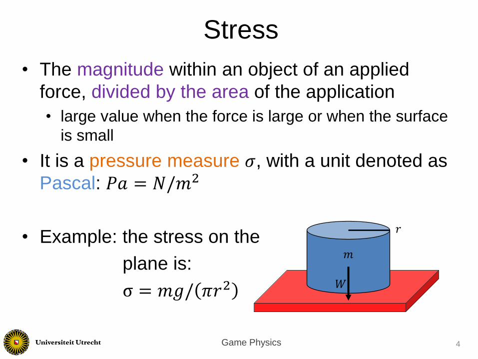
• The magnitude within an object of an applied

force, divided by the area of the application

• large value when the force is large or when the surface

is small

• It is a pressure measure 𝜎, with a unit denoted as

Pascal: 𝑃𝑎 = 𝑁/𝑚2

• Example: the stress on the

plane is:

σ = 𝑚𝑔/ 𝜋𝑟2

4

Stress

𝑟

𝑊

𝑚

Game Physics

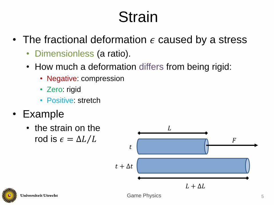
• The fractional deformation 𝜖 caused by a stress

• Dimensionless (a ratio).

• How much a deformation differs from being rigid:

• Negative: compression

• Zero: rigid

• Positive: stretch

• Example

• the strain on the

rod is 𝜖 = ∆𝐿 𝐿

5

Strain

𝐹𝑡

𝑡 + ∆𝑡

𝐿

𝐿 + ∆𝐿

Game Physics

• The amount of stress to produce a strain is a

property of the material.

• Modulus: a ratio of stress to strain.

• Usually in a linear direction, along a planar region or

throughout a volume region.

• Young’s modulus, Shear modulus, Bulk modulus

• Describing the material reaction to stress.

6

Body Material

Game Physics

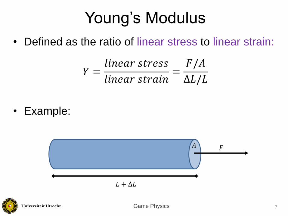
• Defined as the ratio of linear stress to linear strain:

𝑌 =𝑙𝑖𝑛𝑒𝑎𝑟 𝑠𝑡𝑟𝑒𝑠𝑠

𝑙𝑖𝑛𝑒𝑎𝑟 𝑠𝑡𝑟𝑎𝑖𝑛=𝐹/𝐴

∆𝐿/𝐿

• Example:

7

Young’s Modulus

𝐿 + ∆𝐿

𝐹𝐴

Game Physics

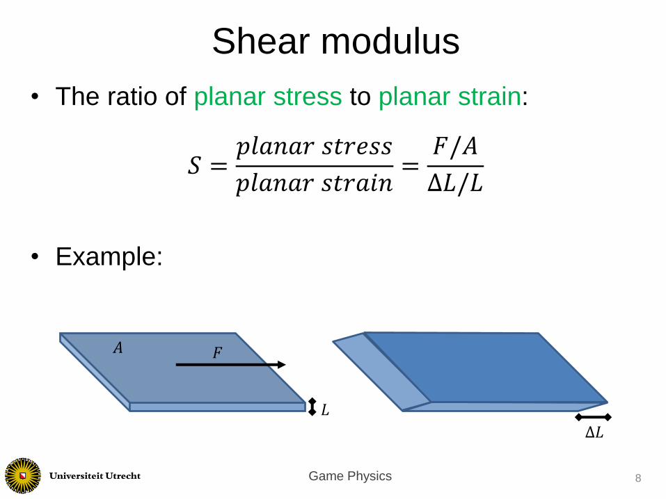
• The ratio of planar stress to planar strain:

𝑆 =𝑝𝑙𝑎𝑛𝑎𝑟 𝑠𝑡𝑟𝑒𝑠𝑠

𝑝𝑙𝑎𝑛𝑎𝑟 𝑠𝑡𝑟𝑎𝑖𝑛=𝐹/𝐴

∆𝐿/𝐿

• Example:

8

Shear modulus

𝐿

𝐴 𝐹

∆𝐿

Game Physics

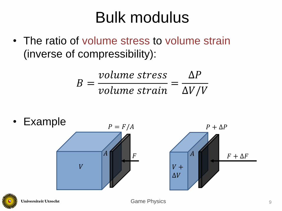
• The ratio of volume stress to volume strain

(inverse of compressibility):

𝐵 =𝑣𝑜𝑙𝑢𝑚𝑒 𝑠𝑡𝑟𝑒𝑠𝑠

𝑣𝑜𝑙𝑢𝑚𝑒 𝑠𝑡𝑟𝑎𝑖𝑛=∆𝑃

∆𝑉/𝑉

• Example

9

Bulk modulus

𝐴

𝑃 = 𝐹/𝐴

𝑉

𝐹 𝐴

𝑃 + ∆𝑃

𝑉 +∆𝑉

𝐹 + ∆𝐹

Game Physics

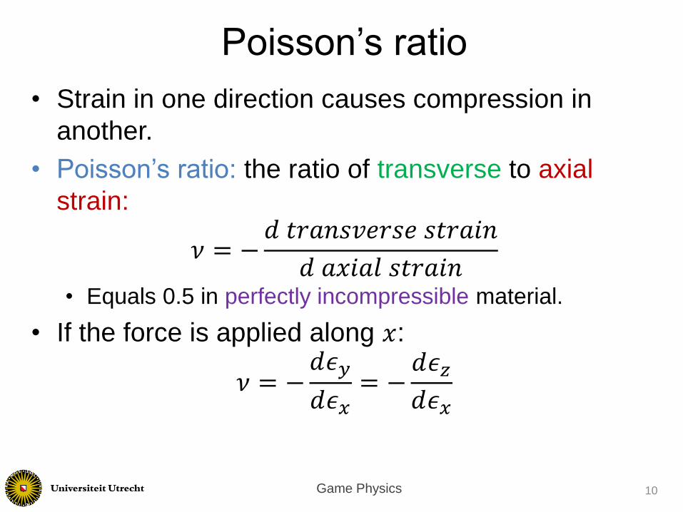
• Strain in one direction causes compression in

another.

• Poisson’s ratio: the ratio of transverse to axial

strain:

𝜈 = −𝑑 𝑡𝑟𝑎𝑛𝑠𝑣𝑒𝑟𝑠𝑒 𝑠𝑡𝑟𝑎𝑖𝑛

𝑑 𝑎𝑥𝑖𝑎𝑙 𝑠𝑡𝑟𝑎𝑖𝑛• Equals 0.5 in perfectly incompressible material.

• If the force is applied along 𝑥:

𝜈 = −𝑑𝜖𝑦

𝑑𝜖𝑥= −𝑑𝜖𝑧𝑑𝜖𝑥

10

Poisson’s ratio

Game Physics

• Example of a cube of size 𝐿

𝑑𝜖𝑥 =𝑑𝑥

𝑥𝑑𝜖𝑦 =

𝑑𝑦

𝑦𝑑𝜖𝑧 =

𝑑𝑧

𝑧

−𝜈 𝐿

𝐿+∆𝐿 𝑑𝑥

𝑥= 𝐿

𝐿−∆𝐿′ 𝑑𝑦

𝑦= 𝐿

𝐿−∆𝐿′ 𝑑𝑧

𝑧⇔

1 +∆𝐿

𝐿

−𝑣

= 1 −∆𝐿′

𝐿⇔ 𝜈 ≈

∆𝐿′

∆𝐿

11

Poisson’s ratio

𝐹

Δ𝐿

𝐿

∆𝐿′

8.1-8.5

Game Physics

• A deformable object is defined by rest shape and

material parameters.

• Deformation map: 𝑞 = 𝑓( 𝑝) of every point 𝑝 =𝑥, 𝑦, 𝑧 .

• Relative displacement field: 𝑓( 𝑝) = 𝑝 + 𝑢( 𝑝)

12

Continuum Mechanics

𝑝

𝑝 + 𝑑𝑝

𝑑𝑝

𝑞

𝑞+ 𝑑𝑞

𝑑𝑞

𝑓(𝑝)

𝑓(𝑝 + 𝑑𝑝)

𝑑𝑝

𝑑𝑢

Game Physics

• The strain and stress are related to the material

deformation gradient tensor 𝐽𝑞, and so to the

displacement field 𝑢.

• The stretch in a unit direction 𝑣 → 𝑣′:

𝑑𝑣′ 2 = 𝑣𝑇∗ 𝐽𝑞𝑇𝐽𝑞 ∗ 𝑣

• 𝐽𝑞𝑇𝐽𝑞 is called the (right) Cauchy-Green strain

tensor.

• Movement is rigid 𝐽𝑞 is orthonormal 𝐽𝑞𝑇𝐽𝑞 =

I No strain!

14

CG Strain Tensor

Game Physics

• And stress tensor from Hooke’s linear material law

𝜎 = 𝐸 ∗ 𝜖

where 𝐸 is the elasticity tensor and depends on the

Young’s modulus and Poisson’s ratio (and more).

15

Stress Tensor

Game Physics

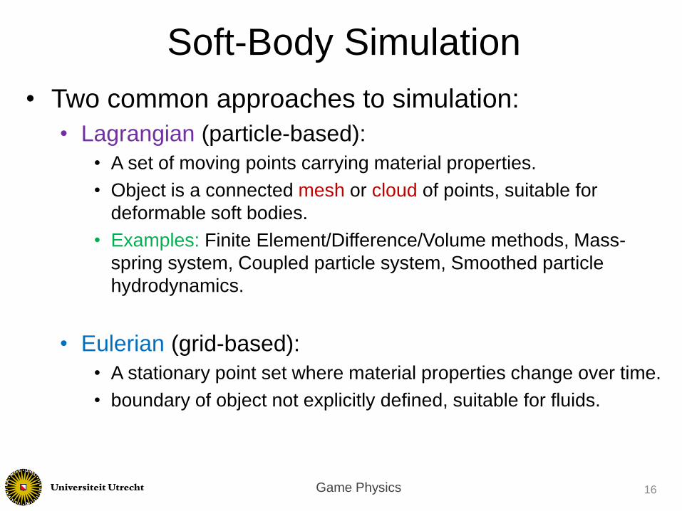
• Two common approaches to simulation:

• Lagrangian (particle-based):

• A set of moving points carrying material properties.

• Object is a connected mesh or cloud of points, suitable for

deformable soft bodies.

• Examples: Finite Element/Difference/Volume methods, Mass-

spring system, Coupled particle system, Smoothed particle

hydrodynamics.

• Eulerian (grid-based):

• A stationary point set where material properties change over time.

• boundary of object not explicitly defined, suitable for fluids.

16

Soft-Body Simulation

Game Physics

• For every point 𝑞, The PDE is given by

𝜌 ∗ 𝑎 = 𝛻 ∙ 𝜎 + 𝐹

• 𝜌: the density of the material.

• 𝑎: acceleration of point 𝑞.

• 𝛻 ∙ 𝜎 = 𝑑 𝑑𝑥 , 𝑑 𝑑𝑦 , 𝑑 𝑑𝑧 ∗ 𝜎 is the divergence

of the stress tensor (internal forces):

• 𝐹: other external forces.

17

Motion of Dynamic Elastic materials

Game Physics

• Used to numerically solve partial differential

equations (PDEs).

• Tessellating the volume into a large finite number

of disjoint elements (3D volumetric/surface mesh).

• Typical workflow:

• Estimating deformation field from nodes.

• Computing local strain and stress tensors

• The motion equation determined by integrating the

stress field over each element.

18

Finite Element Method (FEM)

Game Physics

• If the object is sampled using a regular spatial grid,

the PDE can be discretized using finite differences.

• Pro: easier to implement than FEM.

• Con: difficult to approximate complex boundaries.

• Semi-implicit integration is used to move forward

through time

19

Finite Differences Method

Game Physics

• The boundary element method simplifies the finite

element method from a 3D volume problem to a

2D surface problem.

• PDE is given for boundary deformation.

• Only works for homogenous material.

• Topological changes more difficult to handle.

21

Boundary Element Method

Game Physics

• An object consists of point masses connected by a

network of massless springs.

• The state of the system: the positions 𝑥𝑖 and

velocities 𝑣𝑖 of the masses 𝑖 = 1⋯𝑛.

• The sum force 𝑓𝑖 on each mass:

• External forces (e.g. gravity, friction).

• Spring connections with the mass’ neighbors.

• The motion equation 𝑓𝑖 = 𝑚𝑖𝑎𝑖 is summed up:

𝑀 ∗ 𝑎 = 𝑓(𝑥, 𝑣)

where 𝑀 is a 3𝑛 × 3𝑛 diagonal matrix.

22

Mass-Spring System

Game Physics

• Mass points are initially regularly spaced in a 3D

lattice.

• The edges are connected by structural springs.

• resist longitudinal deformations

• Opposite corner mass points are connected by

shear springs.

• resist shear deformations.

• The rest lengths define the rest shape of the

object.

23

Mass-Spring System

Game Physics

• The force acting on mass point 𝑖 generated by the

spring connecting 𝑖 and 𝑗 is

𝑓𝑖 = 𝐾𝑠𝑖( 𝑥𝑖𝑗 − 𝑙𝑖𝑗)𝑥𝑖𝑗

𝑥𝑖𝑗

where 𝑥𝑖𝑗 is the vector from positions 𝑣𝑖to 𝑣𝑗, 𝐾𝑖 is

the stiffness of the spring and 𝑙𝑖𝑗 is the rest length.

• To simulate dissipation of energy, a damping force

is added:

𝑓𝑖 = 𝐾𝑑𝑖𝑣𝑗 − 𝑣𝑖

𝑇𝑥𝑖𝑗

𝑥𝑖𝑗𝑇𝑥𝑖𝑗

𝑥𝑖𝑗

24

Mass-Spring System

Game Physics

• Pro: intuitive and simple to implement.

• Con: Not accurate and does not necessarily

converges to correct solution.

• depends on the mesh resolution and topology

• …and the choice of spring constants.

• Can be good enough for games, especially cloth

animation

• For possible strong stretching resistance and weak

bending resistance.

25

Mass-Spring System

Game Physics

• Particles interact with each other depending on

their spatial relationship.

• these relationships are dynamic, so geometric and

topological changes can take place.

• Each particle 𝑝𝑖 has a potential energy 𝐸𝑃𝑖.

• The sum of the pairwise potential energies between the

particle 𝑝𝑖 and the other particles.

𝐸𝑃𝑖 =

𝑗≠𝑖

𝐸𝑃𝑖𝑗

26

Coupled Particle System

Game Physics

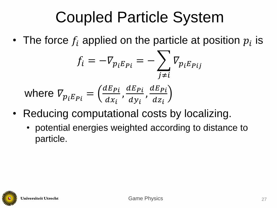
• The force 𝑓𝑖 applied on the particle at position 𝑝𝑖 is

𝑓𝑖 = −𝛻𝑝𝑖𝐸𝑃𝑖 = −

𝑗≠𝑖

𝛻𝑝𝑖𝐸𝑃𝑖𝑗

where 𝛻𝑝𝑖𝐸𝑃𝑖 =𝑑𝐸𝑃𝑖

𝑑𝑥𝑖,𝑑𝐸𝑃𝑖

𝑑𝑦𝑖,𝑑𝐸𝑃𝑖

𝑑𝑧𝑖

• Reducing computational costs by localizing.

• potential energies weighted according to distance to

particle.

27

Coupled Particle System

Game Physics

• The equation for any quantity 𝐴 at any point 𝑟 is given by

𝐴 𝑟 =

𝑗

𝑚𝑗𝐴𝑗

𝜌𝑗𝑊( 𝑟 − 𝑟𝑗 , ℎ)

• 𝑊 is a smoothing kernel.– usually Gaussian function or cubic spline.

• ℎ the smoothing length (max influence distance).

• Example: the density can be calculated as

𝜌 𝑟 =

𝑗

𝑚𝑗𝑊( 𝑟 − 𝑟𝑗 , ℎ)

• It is applied to pressure and viscosity forces, while external forces are applied directly to the particles.

28

Smoothed Particle Hydrodynamics

Game Physics

• Derivatives of quantities: by derivatives of 𝑊.

• Varying the smoothing length ℎ tunes the

resolution of a simulation locally.

• Typically use a large length in low particle density

regions and vice versa.

• Pro: easy to conserve mass (constant number of

particles).

• Con: difficult to maintain material incompressibility.

29

Smoothed Particle Hydrodynamics

Game Physics

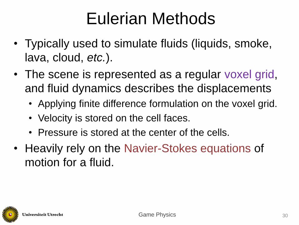
• Typically used to simulate fluids (liquids, smoke,

lava, cloud, etc.).

• The scene is represented as a regular voxel grid,

and fluid dynamics describes the displacements

• Applying finite difference formulation on the voxel grid.

• Velocity is stored on the cell faces.

• Pressure is stored at the center of the cells.

• Heavily rely on the Navier-Stokes equations of

motion for a fluid.

30

Eulerian Methods

Game Physics

• Representing the conservation of mass and momentum for an incompressible fluid:

𝛻 ∙ 𝑢 = 0

𝜌 𝑢𝑡 + 𝑢 ∙ 𝛻𝑢 = 𝛻 ∙ 𝜈 𝛻𝑢 − 𝛻𝑝 + 𝑓

• 𝑢𝑡 is the time derivative of the fluid velocity (the unknown), 𝑝 is the pressure field, 𝜈 is the kinematic viscosity, 𝑓 is the body force per unit mass (usually just gravity ρ𝑔).

31

Navier-Stokes Equations

Inertia (per volume) Divergence of stress

Unsteady

acceleration

Convective

acceleration

Pressure

gradientViscosity

Other body

forces

Game Physics

• First 𝑓 is scaled by the time step and added to the

current velocity

• Then the advection term 𝑢 ∙ 𝛻𝑢 is solved

• it governs how a quantity moves with the underlying

velocity field (time independent, only spatial effect).

• it ensures the conservation of momentum.

• sometimes called convection or transport.

• solved using a semi-Lagrangian technique.

32

Navier-Stokes Equations

Game Physics

• Then the viscosity term 𝛻 ∙ 𝜈 𝛻𝑢 = 𝑣𝛻2𝑢 is solved

• it defines how a cell interchanges with its neighbors.

• also referred to as diffusion.

• Viscous fluids can be achieved by applying diffusion to

the velocity field.

• it can be solved for example by FD and an explicit

formulation:

• 2-neighbor 1D:

𝑢𝑖(𝑡) = 𝑣 ∗ ∆𝑡 ∗ 𝑢𝑖+1 + 𝑢𝑖−1 − 2𝑢𝑖

• 4-neighbor 2D: 𝑢𝑖,𝑗 𝑡 = 𝑣 ∗ ∆𝑡 ∗ 𝑢𝑖+1,𝑗 + 𝑢𝑖−1,𝑗 + 𝑢𝑖,𝑗+1 +

33

Navier-Stokes Equations

Game Physics

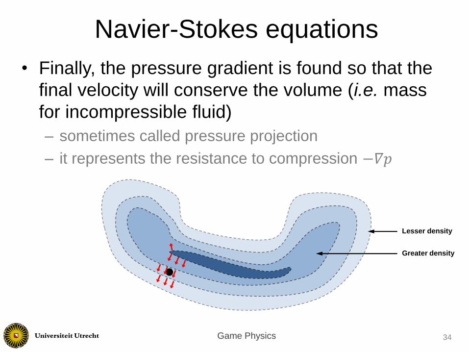
• Finally, the pressure gradient is found so that the

final velocity will conserve the volume (i.e. mass

for incompressible fluid)

– sometimes called pressure projection

– it represents the resistance to compression −𝛻𝑝

34

Navier-Stokes equations

Lesser density

Greater density

Game Physics

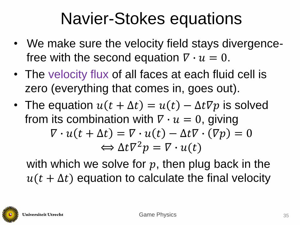
• We make sure the velocity field stays divergence-

free with the second equation 𝛻 ∙ 𝑢 = 0.

• The velocity flux of all faces at each fluid cell is

zero (everything that comes in, goes out).

• The equation 𝑢 𝑡 + ∆𝑡 = 𝑢 𝑡 − ∆𝑡𝛻𝑝 is solved

from its combination with 𝛻 ∙ 𝑢 = 0, giving

𝛻 ∙ 𝑢 𝑡 + ∆𝑡 = 𝛻 ∙ 𝑢 𝑡 − ∆𝑡𝛻 ∙ 𝛻𝑝 = 0⟺ ∆𝑡𝛻2𝑝 = 𝛻 ∙ 𝑢(𝑡)

with which we solve for 𝑝, then plug back in the

𝑢(𝑡 + ∆𝑡) equation to calculate the final velocity

35

Navier-Stokes equations

Game Physics

• Compressible fluids can also conserve mass, but

their density must change to do so.

• Pressure on boundary nodes

• In free surface cells, the fluid can evolve freely (𝑝 = 0)• so that for example a fluid can splash into the air

• Otherwise (e.g. in contact with a rigid body), the fluid

cannot penetrate the body but can flow freely in

tangential directions 𝑢𝑏𝑜𝑢𝑛𝑑𝑎𝑟𝑦 ∙ 𝑛 = 𝑢𝑏𝑜𝑑𝑦 ∙ 𝑛.

36

Navier-Stokes equations

End of

Soft body physics

Next

Physics engine design and

implementation