and at the same time keeping the watertable at sufficient depth. If natural drainage and seepage can be neglected, the drain discharge will probably be in the following ranges (FAO 1980):

- Less than 1.5 mm/d: For soils with a low infiltration rate; - 1.5-3.0 mm/d: For most soils, with the higher rate for more permeable soils

and where cropping intensity is high; - 3.0-4.5 mm/d: For extreme conditions of climate, crop, and salinity

management, and under poor irrigation practices; - More than 4.5 mm/d: For special conditions (e.g. rice irrigation on lighter-textured

soils).

15.7 Sodium Hazard of Irrigation Water

15.7.1 No Precipitation of Calcium Carbonate

In Section 15.2.2, the relationship was shown between the exchangeable sodium of the adsorption complex of the soil, expressed by the ESP, and the ratio between sodium and calcium plus magnesium present in the soil solution, expressed by the SAR. The SAR is therefore also used to express the sodium hazard of irrigation water, but this does not mean that the SAR of the soil solution is equal to the SAR of the irrigation water, even in the absence of exchange or precipitation reactions. An increase in soil water concentration causes the SAR to increase in proportion to the square root of the concentration factor

= &.SAR, n.Na, SAR,,,, water = (15.43)

Table 15.16 presents the ionic composition of the saline waters used in the water- quality test mentioned in Figure 15.25 and Table 15.12, and the relationship between ESP and SAR. The values of ESP and SAR are averages of the layer 0-0.40 m over a period of 4 years, during which the values increased slightly during summer and decreased during the rainy winter season. In Table 15.16, a good correlation appears between ESP and SAR,, the ESP-values being slightly lower than the values calculated from SAR, according to Equation 15.3. Since part of the water is provided by rainfall, the average concentration of the water applied equals 0.7 times (i.e 1000/1400) that of the irrigation water and SAR,,, = J0.7 SAR,. The ratio between SAR, and SARi+,, equalling Jn, ranges around 1.5 and points towards a value between 2 and 2.5.for the concentration factor of the extract of the saturated paste.

15.7.2 Precipitation of Calcium Carbonate

Equation 15.43 for the relation between the SAR of soil water and the SAR of irrigation water holds true if there is no precipitation of salts. Irrigation waters often contain appreciable amounts of calcium and bicarbonate or even carbonate ions,

580

Table 15.16 Composition of saline waters used in water-quality test and relationship between ESP and SAR

~ ~~

Water quality

B C D K + Na+ Ca2 +

Mg2f HCO; Cl - so;- cto t EC

o. 1 11.5 6.0 2.8 1.6

11.5 7.1

20.3 2.1

0.2 21 .o 10.3 5.0 2.2

21.1 13.1 36.5 3.5

2.5 29.6 15.7 8.6 2.6

31.8 20.3 55.6 5.2

ESP (-> 6.7 7.8 8.8

SARi V") 5.5 ,I 7.5 8.5 SAR, +p Vmeq/l) 4.6 6.2 7.0 SAR,/SARi+, (-) 1.6 1.4 1.4

SAR, Vmedl) 7.4 8.5 9.5

which, upon concentration in soil water, precipitate as calcium carbonate. In Table 15.4a, it was shown that the solubility of CaCO, depends on carbon dioxide pressure and total concentration of dissimilar ions. Under average soil conditions it may be set between 5 and 10 meq/l.

For a more exact appraisal of the precipitation of CaCO, and the sodium hazard of irrigation water, the solubility of CaCO, can be determined with the graph of Figure 15.26, which is based on data published by Bower et al. (1965), who made use of earlier studies by Langelier in 1936. The chemical reactions involved are the following

- CO2 + H2O e H2CO3 [HzCO~I = cpc02 '

- H,CO, e H+ + HCO;

- HCOj g H+ + CO:-

- CaCO, g Ca2+ + CO:- K, = [Ca2+] [CO:-]

in which C is a constant, KI and K2 represent dissociation constants, K, the solubility product, and brackets denote ion activities. To convert ion activity into concentration, the Debije-Hückel correction is introduced on the right-hand axis of the graph. This correction depends on the total salt concentration of the solution, C,,,.

If the concentrations of Ca2+ and HC03- are equal (e.g. when water not containing Ca2+ and HCO,- is brought into contact with solid CaCO,), the solubility of CaC0, is found by selecting, on the right-hand axis, the appropriate combination of CO2-

58 1

Ca2+in meq/l

0.7

25

30

40

""i

:

-

1.5 t L

2.0 t L

2.5 1

HC - .

in meqll

- Ctot in meqll 30

15

10

3.0

2.0

3.0 /- ,

5.0

6.0

I

50

Figure 15.26 Equilibrium H20-C02-CaC03 at 25°C according to Langelier-Bower

pressure and total concentration of the solution. A straight line is drawn through this point in such a way that it intersects the Ca-axis and the HC0,-axis at equal values. As an example, if P-CO, = 1000 Pa (corresponding with 1% of CO2 in the soil air) and the total salt concentration of the soil solution C,,, = 60 meq/l, one finds that the concentrations of both components are 5 meq/l (solid line in Figure 15.26). The data presented in Table 15.4a were obtained in this way.

If, in the solution, a difference exists between the concentration of Ca2+ and HCOq, this difference will persist after precipitation. As precipitation occurs as CaCO,, each meq of Ca2+ takes away 1 meq of HC0,- (stochiometric precipitation). As an example, let us take irrigation water with a total salt concentration of 22 meq/l, 3.6 meq/l Ca2+, and 4.0 meq/l HC03-. For a leaching fraction of 0.2, the soil water becomes five times

582

as concentrated, which would mean 18 meq/l CaZ+ and 20 meq/l HC0,- if there were no precipitation. This difference of 2 meq/l in favour of HCO, will persist after precipitation. Thus for P-COz equalling 1000 Pa and C,,, = 100 meq/l, one finds 6.2 meq/l HC0,-and 4.2 meq/l Ca2+ (dotted line in Figure 15.26).

The precipitation of slightly soluble salts has two effects: - A favourable effect on total salinity: the total concentration will be lower than it

- An unfavourable effect on the sodium hazard: the relative concentration of Na+ would have been if all the salts had remained in solution;

increases, as does the SAR-value.

To take into account the precipitation of slightly soluble carbonate from irrigation water, Eaton (Richards 1954) developed the residual sodium carbonate or RSC concept. The RSC-value is defined as (HC03- + CO:-) (Caz+ + Mg2+), expressed in meq/l. On the basis of the RSC, Eaton presented the following classification of irrigation water: -

- 1.25 < RSC < 2.5 : Irrigation water marginal; -

RSC > 2.5 : Irrigation water not suitable;

RSC < 1.25: Irrigation water probably safe.

This classification was considered tentative. And indeed, it appears that sometimes waters with higher RSC-values than indicated. can be used without serious problems for soil structure and permeability.

In Eaton’s experiments, only calcium and sodium were applied as cations. Calcium and magnesium are often determined together and are referred to as Ca + Mg in the composition of irrigation waters. It is questionable, however, whether magnesium should be taken into account in evaluating the precipitation of carbonates. In irrigated soils under normal conditions, magnesium does not precipitate as magnesium carbonate (Suarez 1975). Magnesium probably precipitates together with calcium and is built into the crystal lattice of calcite. It is often found as an impurity in aragonite and calcite, two modifications of solid calcium carbonate.

Although Eaton’s classification of waters by their RSC-value may not be correct, the RSC-value is still useful as a warning signal that the SAR of the soil solution may increase strongly, exceeding by far the normal increase proportional to the square root of the concentration factor. In the case of a positive RSC-value, the procedure presented in the next sections is more accurate and gives more insight into the SAR of the soil solution that might be expected.

15.7.3 Examples of Irrigation Waters containing Bicarbonate

We shall demonstrate the effect of the precipitation of bicarbonates by gradually concentrating irrigation water of the Ca(HC03)2 type and of low salt concentration with an ECi of 0.45 dS/m (Table 15.17). A IO-fold increase in concentration (Line 2) will cause Caz+ to precipitate as carbonate. We can then approximate the equilibrium concentration of Ca2+ and HCO; with the help of Figure 15.26, keeping in mind that the difference in concentration of Ca2+ (38 meq/l) and HCO; (36 meq/l)

583

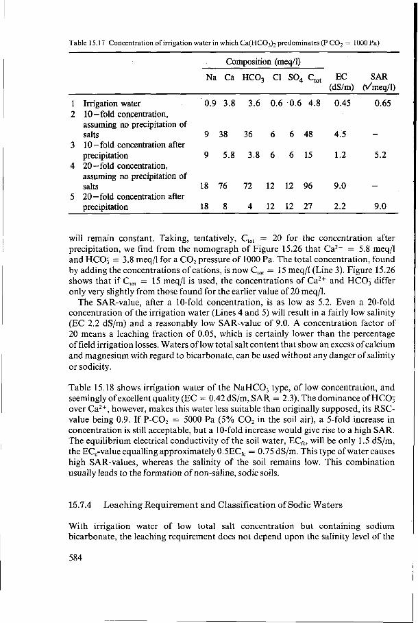
Table 15.17 Concentration of irrigation water in which Ca(HC03), predominates (P CO2 = 1000 Pa)

Composition (meq/l)

Na Ca HCO, C1 SO, C,, EC S A R (dS/m) Mmedl)

1 Irrigation water 0.9 3.8 3.6 0.6 .0.6 4.8 0.45 0.65 2 10-fold concentration,

assuming no precipitation of salts 9 38 36 6 6 48 4.5 -

3 10 -fold concentration after precipitation 9 5.8 3.8 6 6 15 1.2 5.2

4 20 -fold concentration, assuming no precipitation of salts

5 20 -fold concentration after 18 76 72 12 12 96 9.0 -

precipitation 18 8 4 12 12 27 2.2 9.0

will remain constant. Taking, tentatively, C,,, = 20 for the concentration after precipitation, we find from the nomograph of Figure 15.26 that Ca2+ = 5.8 meq/l and HCO; = 3.8 meq/l for a CO2 pressure of 1000 Pa. The total concentration, found by adding the concentrations of cations, is now C,,, = 15 meq/l (Line 3). Figure 15.26 shows that if C,,, = 15 meq/l is used, the concentrations of Ca2+ and HCOj differ only very slightly from those found for the earlier value of 20 meq/l.

The SAR-value, after a 10-fold concentration, is as low as 5.2. Even a 20-fold concentration of the irrigation water (Lines 4 and 5) will result in a fairly low salinity (EC 2.2 dS/m) and a reasonably low SAR-value of 9.0. A concentration factor of 20 means a leaching fraction of 0.05, which is certainly lower than the percentage of field irrigation losses. Waters of low total salt content that show an excess of calcium and magnesium with regard to bicarbonate, can be used without any danger of salinity or sodicity.

Table 15.18 shows irrigation water of the NaHC03 type, of low concentration, and seemingly of excellent quality (EC = 0.42 dS/m, SAR = 2.3). The dominance of HCO, over Ca2+, however, makes this water less suitable than originally supposed, its RSC- value being 0.9. If P-CO2 = 5000 Pa (5% CO2 in the soil air), a 5-fold increase in concentration is still acceptable, but a 10-fold increase would give rise to a high SAR. The equilibrium electrical conductivity of the soil water, ECfc, will be only 1.5 dS/m, the EC,-value equalling approximately 0.5ECfc = 0.75 dS/m. This type of water causes high SAR-values, whereas the salinity of the soil remains low. This combination usually leads to the formation of non-saline, sodic soils.

15.7.4 Leaching Requirement and Classification of Sodic Waters

With irrigation water of low total salt concentration but containing sodium bicarbonate, the leaching requirement does not depend upon the salinity level of the

584

I

Composition (meq/l)

Na Ca HCO, C1 SO, C,, EC SAR

1 Irrigation water 2.5 2.4 3.3 1.3 0.5 5.0 0.42 2.3 2 5 -fold concentration,

(dS/m) (dmeq/l)

assuming no precipitation of salts 12.5 12.0 16.5 6.5 2.5 25.0 2.1 -

3 5 -fold concentration after precipitation 12.5 4.5 9.0 6.5 2.5 17.5 1.5 8.3

assuming no precipitation of

5 10-fold concentration after

1 4 10-fold concentration,

salts 25 24 33 13 5 50 4.2 -

DreciDitation 25 3 12 13 5 29 2.4 20.4

soil but on its sodicity level. We can estimate the sodicity level of the soil, expressed by the SAR of the soil water, by concentrating the irrigation water while taking into account the precipitation of calcium carbonate. If calcium and magnesium are determined together, we can then use, as an approximation, the concentration of both cations, instead of calcium only, in the nomograph of Figure 15.26. A second approximation concerns the carbon dioxide pressure of the soil air. It depends upon depth, root activity, and organic matter content. We can estimate a range for the SAR- value of the soil water by assuming P-CO,-values of 1000 and 5000 Pa, the lower value being more representative for the tilled layer and the higher value for the soil at greater depth.

The permissible SAR-value of the soil water depends upon soil salinity, texture, and clay minerals, and upon the farmers’ capacity to till to counteract an unfavourable soil structure. Tentatively, the SAR value can be put between 15 and 25 for the soil water at field capacity, but this has to be checked for local conditions.

As long as the permissible concentration factor is higher than 4 to 5 , percolation losses of 0.20-0.25 will provide sufficient leaching for sodicity control. If the concentration factor appears to be lower, the farmer should not increase the water applications to provide more leaching because this may lead to excessive watering and yield depression due to water stagnating on the surface. A better solution to improve the unfavourable salt composition and the high SAR-value of the irrigation water is to apply amendments (e.g. gypsum) to the soil or the irrigation water, or to blend the irrigation water with water of better quality.

A high SAR-value is more dangerous than a high salt concentration, because it affects the permeability of the soil, which is the key to the leaching process. Sodic waters affect the structure and the permeability of the soil through their effects on the cation exchange complex. We need therefore only take the sodium hazard into account for soils in which the exchange capacity is large enough to affect the soil structure. In sand and loamy sand, the clay fraction is so small that the sodium hazard of irrigation water is not a factor to be reckoned with.

585

Table 15.19 Leaching fraction of bicarbonate waters calculated with Figure 15.26 (PCO, = 1000 Pa)

Composition (meq/l)

n LF Na Ca Mg HCO, Cl+SO, Ctot SAR RSC

Irr. water A l 3.5 0.7 O 3.3 0.9 4.2 5.9 2.6 Soil water 3.5 0.28 12.3 0.75 O 9.9 3.1 13.0 20 Irr. water A2 3.5 0.35 0.35 3.3 0.9 4.2 5.9 2.6 Soil water 6.4 0.16 22.4 0.3 2.2 19.2 5.8 25.0 20

Irr. water B1 9.4 1.7 O 7.1 4.0 1 1 . 1 10.2 5.4 Soil water 1.5 0.67 14.1 1.0 O 9.1 6.0 15.1 20 Irr. water B2 9.4 0.85 0.85 7.1 4.0 11.1 10.2 5.4 Soil water 2.3 0.43 21.6 0.45 1.95 14.8 9.2 24.0 20

1rr.-water C1 3.3 0.2 o 1.1 2.4 3.5 10.4 0.9 Soil water 3.7 0.27 12.2 0.74 O 4.1 8.9 13.0 20 Irr. water C2 3.3 0.1 0.1 1.1 2.4 3.5 10.4 0.9 Soil water 3.7 0.27 12.2 0.37 0.37 4.1 8.9 13.0 20

Table 15.19 presents the concentration factor and leaching fraction calculated with Figure 15.26 for three waters, under assumptions of a P-C02 of 1000 Pa and 20 as a limit for the SAR of the soil water. In the calculations, two approaches are followed: - Calcium and magnesium are taken together for precipitation (Irr. water Al, B, and

- Calcium and magnesium are separated into equal concentrations and magnesium

The second approach leads to a higher concentration factor, except for water C, in which calcium does not even attain its solubility limit. The low concentration factor of water B corresponds well with its high RSC-value, indicating that this water cannot be used without amendments or blending. For water A, the concentration factor is rather low if we assume magnesium and calcium to precipitate together. Still, it can probably be used without serious problems since the leaching fraction of 0.28 is easily obtained in the top layer and the leaching requirement at greater depth is lower owing to the increased pressure of carbon dioxide and the higher solubility of calcium.

Although the RSC of water C is much lower than the RSC of water A, the concentration factor is about the same because of the very low calcium concentration. In this case, the SAR gives a much better indication of the sodium hazard than the RSC.

C1;

does not precipitate (Irr. water A,, B, and C,).

Another procedure for classifying irrigation waters was proposed by FAO (1985). It adapts the approach of Suarez (1981) and introduces an adjusted Sodium Adsorption Ratio to predict potential infiltration problems due to relatively high sodium or low calcium concentrations in the irrigation water.

Na adj.R,, =

586

(1 5.44)

in which

Na = sodium concentration of irrigation water (meq/l) Ca, = calcium concentration (meq/l), modified, according to Table 15.20,

because of the EC of the irrigation water, its HCO;/Ca2+ ratio, and the estimated carbon dioxide pressure in the surface millimetres of the soil (70 Pa)

Mg = magnesium concentration of irrigation water (meq/l)

The adjusted RNa, which predicts the SAR of the soil water near the surface, can be used instead of the SAR of the irrigation water to evaluate potential infiltration problems according to Table 15.21.

Table 15.20 Calcium concentration (Ca,) in meq/l in near-surface soil water after irrigation with water of given HC03/Ca ratio and ECi (FAO 1985)

~

Ratio of HCO,/ (dSlm)

Ca

Salinity of applied water (ECi)

0.1 0.2 0.3 0.5 0.7 1.0 1.5 2.0 3.0 4.0 6.0 8.0

.O5

.10

.15

.20

.25

.30

.35

.40

.45 S O .75

1 .o0

1.25 1.50 1.75 2.00

2.25 2.50 3 .O0 3.50

4 .O0 4.50 5.00 7.00

10.00 20.00

13.20 13.61 8.31 8.57 6.34 6.54 5.24 5.40

4.51 4.65 4.00 4.12 3.61 3.72 3.30 3.40

3.05 3.14 2.84 2.93 2.17 2.24 1.79 1.85

1.54 1.59 1.37 1.41 1.23 1.27 1.13 1.16

1.04 1.08 0.97 1.00 0.85 0.89 0.78 0.80

0.71 0.73 0.66 0.68 0.61 0.63 0.49 0.50

0.39 0.40 0.24 0.25

13.92 14.40 14.79 15.26 15.91 16.43 17.28 17.97 19.07 19.94 8.77 9.07 9.31 9.62 10.02 10.35 10.89 11.32 12.01 12.56 6.69 6.92 7.11 7.34 7.65 7.90 8.31 8.64 9.17 9.58 5.52 5.71 5.87 6.06 6.31 6.52 6.86 7.13 7.57 7.91

4.76 4.92 5.06 5.22 5.44 5.62 5.91 6.15 6.52 6.82 4.21 4.36 4.48 4.62 4.82 4.98 5.24 5.44 5.77 6.04 3.80 3.94 4.04 4.17 4.35 4.49 4.72 4.91 5.21 5.45 3.48 3.60 3.70 3.82 3.98 4.11 4.32 4.49 4.77 4.98

3.22 3.33 3.42 3.53 3.68 3.80 4.00 4.15 4.41 4.61 3.00 3.10 3.19 3.29 3.43 3.54 3.72 3.87 4.11 4.30 2.29 2.37 2.43 2.51 2.62 2.70 2.84 2.95 3.14 3.28 1.89 1.96 2.01 2.09 2.15 2.23 . 2.35 2.44 2.59 2.71

1.63 1.68 1.73 1.78 1.86 1.92 2.02 2.10 2.23 2.33 1.44 1.49 1.53 1.58 1.65 1.70 1.79 1.86 1.97 2.07 1.30 1.35 1.38 1.43 1.49 1.54 1.62 1.68 1.78 1.86 1.19 1.23 1.26 1.31 1.36 1.40 1.48 1.54 1.63 1.70

1.10 1.14 1.17 1.21 1.26 1.30 1.37 1.42 1.51 1.58 1.02 1.06 1.09 1.12 1.17 1.21 1.27 1.32 1.40 1.47 0.91 0.94 0.96 1.00 1.04 1.07 1.13 1.17 1.24 1.30 0.82 0.85 0.87 0.90 0.94 0.97 1.02 1.06 1.12 1.17

0.75 0.78 0.80 0.82 0.86 0.88 0.93 0.97 1.03 1.07 0.69 0.72 0.74 0.76 0.?9 0.82 0.86 0.90 0.95 0.99 0.65 0.67 0.69 0.71 0.74 0.76 0.80 0.83 0.88 0.93 0.52 0.53 0.55 0.57 0.59 0.61 0.64 0.67 0.71 0.74

0.41 0.42 0.43 0.45 0.47 0.48 0.51 0.53 0.56 0.58 0.26 0.26 0.27 0.28 0.29 0.30 0.32 0.33 0.35 0.37

30.00 0.18 0.19 0.20 0.20 0.21 0.21 0.22 0.23 0.24 0.25 0.27 0.28

587

Table 15.21 Guidelines for infiltration problems (after FAO 1985)

SAR ECi (dS/m)

None Slight-to-moderate Severe

0 - 3 > 0.7 0.7 - 0.2 < 0.2 3 - 6 > 1.2 1.2 - 0.3 < 0.3 6 - 12 > 1.9 1.9 - 0.5 < 0.5

12 - 20 > 2.9 2.9 - 1.3 < 1.3 20 - 40 > 5.0 5.0 - 2.9 < 2.9

Tabel 15.22 Calculation of the adjusted RN, of bicarbonate waters and classification with regard to infiltration problems

Irrigation EC, Ca Mg HC03/Ca Ca, adj.RNa Problem water dS/m meq/l meg/l meq/l

Al 0.4 0.7 O 4.7 0.68 6.0 Moderate A2 0.35 0.35 9.4 0.44 5.6 Moderate

B1 1 . 1 1.7 O 4.2 0.80 14.8 Severe B2 0.85 0.85 8.4 0.51 11.3 Moderate to

severe c1 0.35 0.2 O 5.5 0.62 5.9 Moderate c 2 0.1 - 0.1 11.0 0.40 6.6 Moderate to

servere

For the irrigation waters in Table 15.19, Table 15.22 presents the calculation of the adjusted RN, and the classification with regard to infiltration problems. The classification corresponds more or less with what could be expected from the leaching fraction calculated in Table 15.19. It should again be stressed that an SAR-value of 20, taken as a criterion for the soil water, and the guidelines proposed in Table 15.21, depend, besides salinity, on texture, clay minerals, and the tillage capacity of the farmer, and should therefore be checked under local conditions.

15.8 Reclamation of Salt-Affected Soils

15.8.1 General Considerations for Reclamation

Before starting with the reclamation of salt-affected soils, one needs answers to several questions: - Does the soil contain soluble salts and what is the exchangeable sodium percentage? - What is the cause of soil salinization? Is it due to the presence of a shallow watertable,

poor quality irrigation water, or the presence of marine sediments? - What are the physical characteristics of the soil? Is the soil coarse-, medium-, or

fine-textured? What is the dominant clay mineral? What is the hydraulic conductivity in the top soil, the subsoil, and the substratum? What changes in soil physical behaviour are to be expected during leaching?

588

In salt-affected soils, a watertable is often present at shallow depth. If so, the first measure to be taken is to install a drainage system to control the watertable. The second measure is to apply irrigation water to leach the salts from the soil. Hence, other questions to be answered are: - Is drainage technically feasible and economically justified? - Is irrigation water available to leach the salts and, more importantly, to enable

sustained agricultural production on the land once reclaimed?

Another problem to be solved is the presence of excessive amounts of exchangeable sodium, either in combination with poor soil structure or not. On this matter, the following questions need to be answered: - Is the application of a chemical amendment needed, an amendment containing

calcium, or a product that enhances the solubility of calcium carbonate if present in the soil?

- How much of the amendment is required? - Is an amendment commercially and economically available? - Which crops and what cropping pattern are to be selected for the reclamation

period?

Adequate answers to the above questions will allow a decision to be made on whether or not to reclaim the land, and if so, whether to install drainage, leach the soils, and apply amendments.

A financial and economic appraisal is part of the decision-making process. It may turn out that, for one or more specific reasons, not reclaiming the land is the best alternative, particularly when the unreclaimed land has at least some production, e.g. as a meadow. The following case may serve as an illustration.

A survey of the salt-affected lands in the irrigated coastal valleys of Peru (Alva et al. 1976) indicated that, in 135 O00 ha, salinization was classified as moderate to severe. The watertable fluctuated between 1 .O m to less than 0.3 m below soil surface. Reclamation was considered necessary for sustained agricultural production. On 45 O00 ha, however, reclamation was assumed to be difficult, if not impossible, for a variety of reasons: - A shortage of water; - Flat topography and poor discharge conditions for drainage water, making the use

- The land prone to inundation, thus requiring river training prior tg reclamation; - Poor soil conditions.

of pump drainage likely;

15.8.2 Leaching Techniques

Saline soils can be leached by ponding water on the field for long periods of time. This has been the traditional method; it is still common practice. Hence, leaching takes place under nearly saturated conditions.

In the past thirty years, many experiments have been conducted to compare the ponding method with intermittent leaching or leaching by sprinkler. With intermittent

589

leaching, water is not applied continuously but at intervals of one or two weeks during which the soil can dry out. Especially for clay soils, this method offers the advantage that cracks form during those intervals and salt is displaced by capillary movement from the interior of the soil aggregates towards the cracks. It is then washed out of the cracks during the next water application. Experimental data generally point towards water saving with intermittent or sprinkler leaching. Less water is needed to achieve the same degree of salt displacement. The amount of water required, however, is only one factor.

A second factor is the uniformity of salt removal. Saline areas are usually being drained prior to leaching. With ponding, more water is generally entering the soil than draining from it. The watertable will rise and will ultimately reach the soil surface. Then, hydrologically speaking, the ponded water case is attained, which means a fully saturated soil with water on the surface. From that moment onwards, the infiltration of water will be distributed unequally over the field, as shown in Figure 15.27, which presents the pattern of flow lines and equipotentials for the ponded water case. A large fraction of water will be infiltrating near the drain, but, further from it, infiltration will be almost negligible. Consequently, salt displacement from the area midway between drains will be less than close to the drains. A more equitable distribution of the infiltration can be obtained by making ridges parallel to the drains to prevent overland flow in the direction of the drains.

A third factor concerns the time required for reclamation, and the labour, supervision, and equipment involved. With intermittent leaching, more time may be required, although less water will be applied. Moreover, that method requires more labour and supervision, while sprinkler application requires special equipment.

The leaching techniques described above are based on the vertical migration of salts dissolved in excess water that percolates through the soil profile towards the watertable or the drain. Differing from this is surface flushing. With this technique, salt is displaced by water moving over the soil surface; hence, there is a lateral transport

Figure 15.27 Flow lines (solid) and equipotential lines (dotted) in the ponded-water case

590

of salts. Surface flushing is sometimes used to remove visible crusts of salt on the surface of salt-affected soils. Experiments have shown that this method is not very effective. Nevertheless, hydrological conditions may be such that surface flushing is the only (economically feasible) technique. This is true in lowland rice cultivation on salt-affected coastal flats. In lowland rice areas, puddling is sometimes practised. With this technique, the soil is stirred with water impounded on the surface, and salts present in the topsoil dissolve. Before the rice is transplanted, the excess water is drained. It was found (De Wolf, after Van Alphen 1983) that 3-4 tons of salt per ha can be carried off in this way. Albeit a minute amount, it may mean the difference between a low level of crop production and crop failure.

Field conditions will determine what method of water application to select. If irrigation water is available abundantly and continuously or if rice can be planted as a reclamation crop, the ponding technique will be suitable. When water is scarce or expensive or when, upon completion of the reclamation, crops will be sprinkler irrigated, the intermittent water application or sprinkler technique will be the logical choice.

15.8.3 Leaching Equations

When saline soils are leached for reclamation, the leaching efficiency coefficient may differ considerably from one case to another because of differences in soil texture, structure, irrigation method, and rainfall. Moreover, saline soils often differ strongly in the salinity of their successive layers. The best way to describe the leaching of saline soils is therefore to consider the soil a more-than-one-layered profile and to take the leaching efficiency coefficient into account.

After the first application of irrigation water, we can assume that the soil water content is approximately at field capacity. The amount of irrigation water will then equal the amount of percolation water. If evaporation cannot be neglected, we can assume evaporation occurring at the soil surface and that the net amount of irrigation water I’ equals I - E. For the salt concentration of the water entering the soil, we can write Ci’ = CiI/I’. Since, under these conditions, fi equals f, (Section 15.5.2), we can write

R = f R + ( l - f ) R (1 5.45)

RC, = fRCrc + (1 - QRCi (1 5.46)

so 1

c, = fCrc + (1 - f)c, (1 5.47)

The leaching process will be illustrated with two theoretical models: a single reservoir with bypass and a series of reservoirs with bypass. We assume that there is no chemical or physical interaction between solute, solution, and soil.

The Single Reservoir with Bypass We can consider the soil profile or the rootzone as a single one-dimensional reservoir. If mixing takes place in the reservoir and if the volume of water in the reservoir is

59 1

I constant (inflow = outflow), the salt balance reads

Ciqdt = C,qdt + WfcdCfc

where

Cfc = average salt concentration of the reservoir solution (meq/l) Ci = concentration of the influent (meq/l) C, = concentration of the effluent (meq/l) q = flow rate through the reservoir (mm/d) Wfc = water stored in the reservoir (mm)

Combining Equations 15.47 and 15.48 yields

Integration between the limits Cfc = Co at time t = O and C, at time t yields

co - ci c, - ci fqt = Wfc In ~

which can also be written as

C, = Ci + (Co - Ci)e-ftr

where

Co = salt concentration of the reservoir solution at time t = O (meq/l) C, = salt concentration of the reservoir solution at time t (meq/l) T = time of residence (d), which equals Wfc/q

(15.48)

(1 5.49)

(15.50)

(1 5.51)

To calculate the amount of efficient leaching water, fqt, to obtain a specified C,, we can use Equation 15.50, whereas the C, that results from applying a specified amount of leaching water follows from Equation 15.51.

If we do not know the leaching efficieny coefficient, f, it can be estimated from measured values of Ci, Co, and C,. The relation between (C,-Ci)/(Co-C,), plotted on a logarithmic scale, and qt should yield a straight line, from which the leaching

fat

Figure 15.28 Leaching process in a single reservoir with bypass

592

efficiency coefficient can be calculated (Figure 15.28). If no straight line is obtained with a series of C, data, this indicates a decrease in the f-value during the leaching process.

The salt concentrations, C (meq/l), in Equations 15.50 and 15.51 can be replaced by electrical conductivities, EC (dS/m). Note that for Co and C, the ECfc needs to be substituted (= 2EC,). How to calculate the amount of leaching water with Equation 15.50 is illustrated in the following example.

Example 15.4 Soil depth D = 1000 mm, Orc = 0.45, EC, = 0.5ECfc, f = 1, EC, = 1 dS/m, (EC,), = 20 dS/m, (EC,), = 4 dS/m, q = 15 "/day. Step 1 Wfc = 0.45 x 1000 = 450 mm (Equation 15.14);

Step2 T = - = 30d;

Step 3 fqt = 450 In (2

450 15

20) - = 773 mm (Equation 15.50) and (2 x 4) - 1

t=-- 773 - 52d. 1 x 15

The Series of Reservoirs with Bypass If the process of leaching is examined more closely, it will be clear that mixing over the entire depth of the rootzone (often 1 m and more) is not very probable. To take into account the limited range over which mixing is effective, we can suppose the soil to consist of different reservoirs (e.g. corresponding with the soil layers at depths of O-0.20,0.20-0.40,0.40-0.60, and 0.60-0.80 m). Each reservoir receives the outflow from the overlying one. If the initial salt concentrations are the same for all the layers, the following expressions are found for the salt concentrations in successive reservoirs of equal volume

1st reservoir:

2nd reservoir:

Ct = Ci + (Co - Ci) e-"D

Cl,l = Ci + (Co - C,)

4th reservoir: Cl" = Ci + (Co - Ci) 1 + - + + e-"r ( : F :;) n = N - l

Nth reservoir: CF = ci + ( co - Ci) X (1 + g) (15.52) n = O

where

n! = 1 x 2 ~ 3 ~ ........... x n

If the initial salt concentrations of the successive layers are different, the following equations are obtained

593

1st reservoir: Cy = Ci + (C: - Ci)

2nd reservoir: Ct' = Ci + (CA' - Ci)e-"F + (Ci - Ci) - e-ftn

C;I1 = Ci + (CAI1 - Ci)e-"P + (CA' - Ci) +-ftp

ft T

ft T 3rd reservoir:

fLt2 + (CA - Ci) ~ 2T2 e-"iT

fN-ltN-l (N- I)!TN-' +

Nth reservoir: = Ci + e-nr {(Cb - Ci)

(1 5.53)

How to calculate the leaching process with Equation 15.53 will be illustrated in the following example.

Example 15.5 The soil profile consists of four layers of 0.25 m each, with EC,-values of 12, 18, 24, and 28 dS/m to a depth of 1.0 m. It is leached by rainfall, for which we assume an f-value of 1. As Of, = 0.5, the amount of soil water in a layer of 0.25 m equals 125 mm. Since t/T = qt/Wfc, we can calculate t/T from the rainfall, qt, and the amount of soil water, Wfc (125 mm). The desalinization is calculated as is shown in Table 15.23 for steps of 80 mm rainfall.

The same type of equations can be developed for more complicated cases (e.g. when the values of the leaching efficiency coefficient or the reservoir volume - the apparent density - are not constant but vary with depth). But then the equations become more complicated too and it is often simpler to use numerical methods.

Since leaching starts with a mixing of irrigation or rain water at concentration Ci with the soil water of the first soil layer (Layer 1) at concentration C,,, the concentration of the soil solution of Layer 1 after mixing can be calculated with

( 1 5.54) aCi + bC,, = (a + b) C,,

where

a = the amount of influent water (mm) b = the amount of soil water in Layer 1 (mm) Ci = salt concentration of influent water (meq/l) C,, = salt concentration of the soil water in Layer 1 (meq/l) C,, = salt concentration of the soil solution of Layer 1 after mixing (meq/l)

If the amount of water retained in Layer 1 is equal to c mm, an amount (a-c) with a concentration C,, percolates into Layer 2 and mixes with its moisture. The concentration of the soil solution in Layer 2 after being mixed, Cx2, can be calculated in the same way

(1 5.55) (a - c)C,, + dCS2 = (a - c + d)C,,

594

Table 15.23 Example ofcalculation with Equation (1 5.53) (Ci = O, f = 1)

1. t/T 0.64 1.28 1.92 2.56 3.20 3.84 4.48 5.12 2. t2/2T2 0.21 0.82 1.84 3.28 5.12 7.37 10.04 13.14 3. t3/6T3 0.04 0.35 1.18 2.80 5.46 9.44 15.06 22.48 4. 0.52 0.27 0.14 0.07 0.04 0.02 0.01 0.00

6. C? = 5 x 4 6.3 3.3 1.8 0.9 0.5 0.3 0.1 0.07 7. COII 18.0 18.0 18.0 18.0 18.0 18.0 18.0 18.0 8 . 5 x 1 7.7 15.3 23.0 30.6 38.4 46.0 53.7 61.4 9 . 7 + 8 25.7 33.3 41.0 48.6 56.4 64.0 71.7 79.4 10. C/I = 9 x 4 13.6 9.3 6.0 3.8 2.3 1.4 0.8 0.5 11. c;II 24.0 24.0 24.0 24.0 24.0 24.0 24.0 24.0 12.7 x 1 11.5 23.0 34.6 46.1 57.6 69.2 80.6 92.2 13. 5 x 2 2.5 9.8 22.1 39.4 61.3 88.4 120.5 157.7 14. 11 + 12 + 13 38.0 56.8 80.7 109.5 142.9 181.6 225.1 273.9 15. C/I1 = 14 X 4 20.0 15.8 11.9 8.4 5.8 3.9 2.5 1.6 16. C:" 28.0 28.0 28.0 28.0 28.0 28.0 28.0 28.0 17. 11 X 1 15.4 30.7 46.1 61.4 77.8 92.2 102.5 122.9 18. 7 x 2 3.8 14.7 33.1 59.0 92.0 132.7 180.7 236.5 19. 5 x 3 0.5 4.2 14.2 33.6 65.3 113.5 180.0 268.4

21. c,'" = 20 x 4 25.2 21.6 17.8 14.0 10.7 7.9 5.6 3.9

5 . c I 12.0 12.0 12.0 12.0 12.0 12.0 12.0 12.0

20. 16 + 17 f 18 + 19 47.7 77.6 121.4 182.0 262.3 366.2 496.9 657.2

where

d = amount of soil water in Layer 2 (mm)

To simplify the calculations (assuming the same conditions as in Example 15.5 and calculated with Equation 15.53), we suppose that: - ci = o; - Bulk density, and consequently Oft, is the same for all layers; - All rainfall percolates through the entire soil profile, the soil not drying out between

successive periods of rainfall, so c = O and W, = b = d.

We then obtain

Layer 0-0.25

LayerO.25-0.50m: 80 x 7.3 + 125 x 18 = (80 + 125)C,, + C,, = 13.8meq/l

m: 125 x 12 = (80 + 125)C,, + C,, = 7.3 meq/l .

Table 15.24 shows the results of the calculations made with: - The aid of Equation 15.53;

595

Table 15.24 Leaching of a soil profile by rainfall

EC - values calculated with Equation 15.53

Layer Before After leaching with in cm leaching

80 mm 160" 240mm 320" 400 mm 480mm 560mm 640"

O - 25 12.0 6.3 3.3 1.8 0.9 0.5 0.3 o. 1 0.07 25 - 50 18.0 13.6 9.3 6.0 3.8 2.3 I .4 0.8 0.5 50 - 75 24.0 20.0 15.8 11.9 8.4 5.8 3.9 2.5 1.6 75 - 100 28.0 25.2 21.6 17.8 14.0 10.7 6.9 5.6 3.9

EC - values calculated with the numerical method (steps of 20 mm)

Layer Before After leaching with in cm leaching

80" 160" 240mm 320mm 400mm 480" 560mm 640"

O - 25 12.0 6.6 3.7 2.0 1 . 1 0.6 0.3 0.2 o. 1 25 - 50 18.0 13.6 9.5 6.4 4. I 2.6 I .6 I .o 0.6 50 - 75 24.0 20.0 15.9 21.1 8.8 6.2 4.3 2.8 1.9 7 5 - 1 0 0 28.0 25.0 21.5 17.9 14.3 11.0 8.1 5.9 4.3

_ _ _ _ _ _ ~

EC - values calculated with the numerical method (steps of 20 mm)

Layer Before After leaching with in cm leaching

80" 160" 240mm 320" 400mm 480" 560" 640"

O - 25 12.0 7.3 4.5 2.7 I .7 1.0 0.6 0.4 0.2 25 - 50 18.0 13.8 10.1 7.2 5. I 3.5 - 2.4 I .6 1 . 1 50 - 75 24.0 20.0 16.1 12.6 9.7 7.3 5.4 3.9 2.8 75 - 100 28.0 24.9 21.5 18.0 14.8 11.9 9.4 7.3 5.5

- The numerical method, taking steps of 20 mm; - The numerical method, taking steps of 80 mm. As is obvious from this table, the smaller the steps, the closer the results of the numerical method are to those obtained with Equation 15.53. In practice, the differences between them are almost negligible.

The main drawback in using the leaching equations is the unknown leaching efficiency coefficient, which, moreover, can change during the leaching process. The first salts washed out are those easily leached from the large pores; then follow the salts from the small pores, and finally those from the interior of the soil aggregates in 'dead-end' pores.

The best way to approach large reclamation projects is therefore to lay out field tests on the different soil types in the project area. These leaching tests can be conducted in large-diameter infiltrometers or by making ridges around small fields of about 10 m2, depending upon the available facilities (e.g. the transport of water). The results of these tests can then be used to estimate the leaching efficiency coefficient and to calculate the leaching requirement for other saline soils in the project.

596

If no data are available, a rule of thumb often used is that 1 foot of soil needs 1 foot of water for desalinization. To reclaim highly saline soils (EC, > 40 dS/m), Reeve et al. (1955) found as a rule of thumb that 80 and 90% of the salts are removed from the top 0.3 m of soil after a water percolation of 0.3 m and 0.6 m respectively. Experimental data often deviate from this rule. Figure 15.29 presents data from two leaching experiments: - Dujailah, Iraq: loam to silty loam (Dieleman 1963); - Chacupe, Peru: clay loam to clay (Alva et al. 1976).

ECe initial

In the Dujailah experiment, the soil was flooded to lower the salinity in the top soil. During the period of flooding, which took 7 days, a depth of water of about 140 mm had percolated through the soil profile. Then, at a ratio R/D = 0.25, a legume crop was planted and reclamation was continued.

Chacupe O 04 Dulailah O 05

In the Chacupe experiment, an initial leaching was applied. Over a period of 2 months, a depth of water of about 130 mm had percolated through the soil profile. Then, at a ratio R/D = 0.20, rice was planted. Crop yield was very low. A second rice crop was sown at a ratio R/D = 1.2, 14 months after the start of the experiment. This crop yielded satisfactorily.

Obviously, the depth of water required and the time needed for reclamation will vary from place to place, depending on: - Soil properties: soil texture, soil structure, soil pore geometry, cracking phenomena,

clay mineralogy, and physico-chemical behaviour of clays; - Initial salt content and the chemical composition of the soluble salts. (In the above-

mentioned experiments, the initial EC, varied from 40-100 dS/m in Dujailah, and from 80- 150 dS/m in Chacupe);

- Salt content and the chemical composition of the water used for leaching (rain or irrigation);

- Leaching technique and the scope for planting a salt-tolerant crop during reclamation.

Figure 15.29 Leaching curves for a soil depth of 0.60 m

.o 'D

597

15.8.4 Chemical Amendments

The reclamation of sodic soils, particularly those that have a textural B horizon with the columnar soil structure (solonetz), is nearly always a time-consuming and often costly affair. These soils can be used for fishponds or rice cultivation. Minute amounts of salts may diffuse into the supernatant water or be removed by water percolating (if any) through the soil profile. In addition, some exchangeable sodium may be removed from the soil. Also, crops other than rice, but tolerant to exchangeable sodium and poor soil structure, can be planted. There are various grasses that still grow well under such conditions. These crops improve the soil, albeit at a slow rate, through the activity of their roots. Root activity and organic matter enhance the solubility of calcium carbonate, which, if present in the soil, makes calcium available to exchange for sodium. In all, however, the reclamation of sodic soils through fishponds or through the cultivation of rice or other crops tolerant to exchangeable sodium is a slow process, usually taking many years.

Saline sodic soils often show a good soil structure at first. After drainage and an initial leaching, when a large portion of the salts has been removed from the topsoil, the breakdown of soil structure becomes evident: the infiltration rate decreases, the process of leaching is slowed down, and the reclamation period is prolonged.

To speed up the reclamation of sodic soils or to avoid the breakdown of soil structure in saline sodic soils, chemical amendments can be applied (Abrol et al. 1988). These products should either contain a source of soluble calcium or should enhance the solubility of calcium carbonate if present in the soil.,

Amendments of the second category are organic matter, sulphur, pyrites, or acid waste products such as pressmuds and waste sulphuric acid. Their application is limited to soils containing CaCO,. Pyrite and sulphur are most frequently used. Upon oxidation, which is a microbiological process, sulphuric acid is formed as a transitional product. It reacts with and dissolves the calcium carbonate in the soil, forming gypsum, which is a rather soluble source of calcium. The oxidation of sulphur takes some time, particularly if the living conditions for the bacteria involved are adverse.

Amendments containing a soluble source of calcium are calcium chloride, gypsum and phosphor-gypsum. Calcium chloride, being hygroscopic, is rather difficult to handle. Phosphor-gypsum is a by-product of factories producing phosphoric acid. It contains 80-90% calcium sulphate and, when dry, is a fine powder-like material. It was found to be very effective in reclaiming sodic soils (Mehta 1983).

The amendment most frequently used in the reclamation of saline sodic and sodic soils is gypsum. It is found in many places in the world and is a waste product of some industries. The quantity of gypsum required can be calculated with Equation 15.56

8.61 (ESP, - ESP,) CEC D ~b

1000 f S D =

where

( 1 5.56)

S, = the amount of gypsum required in a layer of D m (ton/ha)

598

D = the depth over which soil structure has to be improved or be prevented from breakdown (m). As soil structure in the topsoil is most prone to deterioration due to the mechanical impact of farm implements, rainfall, or irrigation water, a D-value varying between O. 1 and 0.3 m is usually taken

pb ESP, = the actual exchangeable sodium percentage as found from laboratory

analysis ESP, = the final exchangeable sodium percentage to be arrived at after

reclamation. ESP, is usually set at 5-10 CEC = the cation exchange capacity (meq/100 g of soil) f = efficiency of the gypsum application (YO)

= the bulk density of the soil (kg/m3)

The efficiency of a gypsum application depends on various factors: - Not all of the gypsum will be used to replace sodium; some of it will replace other

- The distribution of gypsum will be irregular (i.e. there is a non-uniform spreading); - Part of the gypsum will be transported with the percolating water into the subsoil,

and will not replace sodium in the topsoil. This phenomenon may be more pronounced in soils rich in soluble sodium chloride. This salt enhances the solubility of gypsum (see Table 15.4b);

cations like Mg and K;

- The fineness of the gypsum (Mehta 1983); - The type of soluble salts present in the soil solution (Alva et al. 1976; Dahiya et

al. 1982).

The efficiency of the gypsum dressing is in the order of 40-70%. From a systematic monitoring of the reclamation of soils inundated with sea water in The Netherlands, it was concluded that the maximum efficiency arrived at was 50% (Van der Molen 1957).

The amount of gypsum required, as calculated with Equation 15.56, may serve as a guideline. If a large amount of gypsum is required, applying it in one single dose is of little use because of its rather low solubility. For instance, an application of 20 ton/ha of gypsum would require a quantity of 10 O00 m3 of water to dissolve it. This represents a layer of water of 1000 mm, a quantity that is often more than applied in one cropping season. There is no consensus on whether gypsum should be incorporated into the soil or not. A top-dressing was advocated in the reclamation of the inundated soils in The Netherlands (Van der Molen 1957). In this way, the gypsum would regenerate the upper few centimetres of the soil, making it less sensitive to the impact of raindrops.

Top-dressed gypsum, particularly when fine particles are used (less than 0.25 mm), is displaced with the irrigation water towards the lower part of the field (Alva et al. 1976). Incorporating the gypsum into a dry soil to a depth of 0.05-0.10 m gave the best results. As part of a package of practices for the reclamation of sodic soils in Northern India (Mehta 1983), it was advocated that the gypsum be applied on a well- prepared but dry soil (viz. prior to the onset of the rainy season). Incorporation may not be necessary.

599

References

Abrol, I.P., J.S.P. Yadav and F.I. Massoud 1988. Salt-affected soils and their management. Soils Bulletin

Alva, C.A., J.G. van Alphen, A. de la Torre and L. Manrique 1976. Problemas de drenaje y salinidad

Biggar, J.W., and D.R. Nielsen 1960. Diffusion effects in miscible displacement occurring in saturated

Bower, C.A., L.V. Wilcox, G.W. Akin and M.G. Keyes 1965. An index of the tendency of CaC03 to

Dahiya, I.S., R.S. Malik, and M. Singh 1982. Reclaiming a saline-sodic sandy loam soil under rice

Dieleman, P.J. (ed.) 1963. Reclamation of salt-affected soils in Iraq. ILRI Publication 1 1 , Wageningen,

FAO 1980. Drainage design factors. Irrigation and Drainage Paper 38. Rome, 52 p. FAO 1985. Water quality for agriculture. Irrigation and Drainage Paper 29, Rev. 1 , FAO, Rome, 174 p. FAO 1988. FAO-Unesco soil map of the world. Revised legend. World Soil Resources report 60, FAO,

FAO-Unesco 1973. Irrigation, drainage, and salinity : An international source book. Hutchinson/FAO/

FAO-Unesco 1974. Soil map of the world 1:5 O00 000. Volume I legend. Unesco, Paris, 59 p. Mehta, K.K. 1983. Reclamation of alkali soils in India. Oxford and IBH Publishing Co., New Delhi. Reeve, R.C., A.F. Pillsbury and L.V. Wilcox 1955. Reclamation of a saline and high boron soil in the

Coachella valley of California. Hilgardia 24, pp. 69-91. Richards, L.A. (ed.) 1954. Diagnosis and improvement of saline and alkali soils. USDA Agric. Handbook

60. Washington, 160 p. Rijtema, P.E. 1969. Soil moisture forecasting. Nota 513. Institute for Land and Water Management

Research, Wageningen, 18 p. Suarez, D.L. 1975. Precipitation of magnesium carbonates. Annual Report of the U.S. Salinity Laboratory.

USDA, kverside, California. Suarez, D.L. 1981. Relation between pH, and sodium adsorption ratio (SAR) and an alternative method

for estimating SAR of soil or drainage waters. Soil Sci. Soc. Amer. J. 45, pp. 469-475. Unesco 1970. Research and training on irrigation with saline water. Tech. Report of UNDP Project, Tunisia

5. Unesco, Paris, 256 p. USDA 1975. Soil taxonomy : A basic system of soil classification for making and interpreting soil surveys.

Agric. Handbook 436, Washington, 754 p. Van Alphen, J.G. 1983. 'Rice in the reclamation of salt-affected soils. Seminar on Ecology and management

of problem soils in Asia. Bangkok Proceedings. Van Hoorn, J.W. 1979. The effect of capillary flow on salinization and the concept of critical depth for

determining drain depth. In: J. Wesseling (ed.). Proceedings of the international drainage workshop. ILRI Publication 25, Wageningen: pp. 686-700.

Van Hoorn, J.W. 1981. Salt movement, leaching efficiency, and leaching requirement. Agr. Water Management 4, pp. 409-428.

Van der Molen, W.H. 1957. The exchangeable cations in soils flooded with sea water. Versl. Landbouwk. Onderz. 63.17. The Hague, 167 p.

39. FAO, Rome, 13 1 p.

en la Costa Peruana. ILRI Bulletin 16 (in Spanish), Wageningen, 116 p.

and unsaturated porous materials. J. of Geophys. Res. 65, pp. 2887-95.

precipitate from irrigation waters. Soil Sci. Soc. Am. Proc., 29, pp. 91-92.

production. Agric. Water Management 5, pp. 61-72.

175 p.

Rome, 119 p.

Unesco, London, 510 p.

..

600