social and economic dimensions of an aging population · the program for research on social and...
TRANSCRIPT

S E D A PA PROGRAM FOR RESEARCH ON
SOCIAL AND ECONOMICDIMENSIONS OF AN AGING
POPULATION
SOCIOECONOMIC INFLUENCES ON THE HEALTHOF OLDER CANADIANS: ESTIMATES BASED ON
TWO LONGITUDINAL SURVEYS
NEIL J. BUCKLEYFRANK T. DENTON
A. LESLIE ROBBBYRON G. SPENCER
SEDAP Research Paper No. 139

For further information about SEDAP and other papers in this series, see our web site: http://socserv2.mcmaster.ca/sedap
Requests for further information may be addressed to:Secretary, SEDAP Research Program
Kenneth Taylor Hall, Room 426McMaster University
Hamilton, Ontario, CanadaL8S 4M4
FAX: 905 521 8232e-mail: [email protected]
October 2005
The Program for Research on Social and Economic Dimensions of an Aging Population (SEDAP) is aninterdisciplinary research program centred at McMaster University with co-investigators at seventeen otheruniversities in Canada and abroad. The SEDAP Research Paper series provides a vehicle for distributingthe results of studies undertaken by those associated with the program. Authors take full responsibility forall expressions of opinion. SEDAP has been supported by the Social Sciences and Humanities ResearchCouncil since 1999, under the terms of its Major Collaborative Research Initiatives Program. Additionalfinancial or other support is provided by the Canadian Institute for Health Information, the CanadianInstitute of Actuaries, Citizenship and Immigration Canada, Indian and Northern Affairs Canada, ICES:Institute for Clinical Evaluative Sciences, IZA: Forschungsinstitut zur Zukunft der Arbeit GmbH (Institutefor the Study of Labour), SFI: The Danish National Institute of Social Research, Social DevelopmentCanada, Statistics Canada, and participating universities in Canada (McMaster, Calgary, Carleton,Memorial, Montréal, New Brunswick, Queen’s, Regina, Toronto, UBC, Victoria, Waterloo, Western, andYork) and abroad (Copenhagen, New South Wales, University College London).
This paper is cross-classified as No. 402 in the McMaster University QSEP Research Report Series
SOCIOECONOMIC INFLUENCES ON THE HEALTHOF OLDER CANADIANS: ESTIMATES BASED ON
TWO LONGITUDINAL SURVEYS
NEIL J. BUCKLEYFRANK T. DENTON
A. LESLIE ROBBBYRON G. SPENCER
SEDAP Research Paper No. 139

1 The work underlying this paper was carried out as part of the SEDAP (Social andEconomic Dimensions of an Aging Population) Research Program supported by the SocialSciences and Humanities Research Council of Canada, Statistics Canada, and the CanadianInstitute for Health Information. Computations were carried at the at the Statistics CanadaResearch Data Centre at McMaster University. We would like to thank the referees for helpfulcomments and suggestions
October 2005
SOCIOECONOMIC INFLUENCES ON THE HEALTH OF OLDER CANADIANS:ESTIMATES BASED ON TWO LONGITUDINAL SURVEYS
Neil J Buckley, Frank T Denton, A Leslie Robb and Byron G Spencer1,
Correspondence:Byron G Spencer, Department of Economics, McMaster UniversityHamilton, Ontario, CanadaL8S 4M4
e-mail: [email protected]: 905 525 9140, extension 24594FAX: 905 521 8232

SOCIOECONOMIC INFLUENCES ON THE HEALTH OF OLDER CANADIANS:ESTIMATES BASED ON TWO LONGITUDINAL SURVEYS
Neil J Buckley, Frank T Denton, A Leslie Robb and Byron G Spencer
Abstract:It is well established that there is a positive statistical relationship between socioeconomic
status (SES) and health but identifying the direction of causation is difficult. This study exploits thelongitudinal nature of two Canadian surveys, the Survey of Labour and Income Dynamics and theNational Population Health Survey, to study the link from SES to health (as distinguished from thehealth-to-SES link). For people aged 50 and older who are initially in good health we examinewhether changes in health status over the next two to four years are related to prior SES, asrepresented by income and education. Although the two surveys were designed for differentpurposes and had different questions for income and health, the evidence they yield with respect tothe probability of remaining in good health is similar. Both suggest that SES does play a role andthat the differences across SES groups are quantitatively significant, increase with age, and are muchthe same for men and women.
Keywords: health transitions, income, education
JEL Classification: I10
Résumé:Le lien statistique entre le statut socio-économique (SSE) et la santé est bien établi, en revanche, lesens de la relation de causalité est plus difficile à mettre en évidence. Cette étude exploite la naturelongitudinale de deux enquêtes canadiennes, l’Enquête sur la dynamique du travail et du revenu(EDTR) et l’Enquête nationale sur la santé de la population (ENSP), afin d’examiner la relation decausalité entre le SSE et la Santé (par opposition à la relation de causalité entre la santé et le SSE).Nous avons examiné une population âgée de 50 ans et plus, initialement en bonne santé, afin dedéterminer si durant les deux à quatre années qui ont suivi, les changements de l’état de santé étaientliés au SSE antérieur, mesuré par le revenu et l’éducation. Bien que les deux enquêtes aient étéconçues avec des objectifs différents et comportent des questions différentes sur le revenu et lasanté, l’analyse de ces dernières aboutit à des conclusions similaires concernant la probabilité derester en bonne santé. On trouve que le SSE joue un rôle déterminant et que les différences entre lesgroupes SSE sont quantitativement significatives, augmentent avec l’âge, et ne diffèrent presque pasentre les hommes et les femmes.
1
October 2005
SOCIOECONOMIC INFLUENCES ON THE HEALTH OF OLDER CANADIANS:
ESTIMATES BASED ON TWO LONGITUDINAL SURVEYS
1. INTRODUCTION
Much research has demonstrated that there is a strong positive relationship between
socioeconomic status (SES) and health status. In the words of Fogel and Lee (2003, p.1),
“individuals from different socioeconomic backgrounds face distressingly different prospects of
living a healthy life”. Understanding that relationship, and identifying the causality behind it, is
difficult: Are people in poor health because they have low SES, or do they have low SES
because of their poor health1? In the language of econometrics, is income an endogenous
variable in a health determination equation and/or health an endogenous variable in an income
determination equation? Establishing the direction of influence in this case is of research
interest, but also of practical importance in the design of effective policies to improve population
health.
In earlier work we proposed a framework of analysis for identifying the influences of
income and education on health while working with Canadian panel data in the context of the
older population (Buckley et al., 2004a). We adopt that framework here, and extend our work by
analysing a second Canadian panel data set and comparing the results with those based on the
first. Our concern continues to be with the socioeconomic determinants of health among the

2
older population, in particular the effects of income and education. We ask whether the chances
that older individuals would remain in good health were improved by having higher incomes and
better education. As in our earlier work we focus on the population aged 50 and older2, where we
anticipate SES would generally have a greater potential impact on health3.
There is a large international literature concerned with the income-health connection,
dating back at least to the 1967 Whitehall Study (Marmot, Rose, Shipley and Hamilton, 1978).
This and subsequent contributions to the literature are ably reviewed by Smith (1999), Benzeval
and Judge (2001), Evans (2002), and Deaton (2002, 2003)4. Smith (1999), among others,
emphasises the difficulty of assessing the direction of causation and cautiously notes, in his
concluding remarks (p. 165), that “... economic resources also appear to impact health outcomes
... [and] innovative methods that help isolate economic and health shocks would be informative
on this vexing issue of causality”.
The Canadian literature on this topic that involves quantitative analysis is quite limited,
reflecting the absence of suitable data, at least until recently. One study, that of Badley, Wang,
Cott and Gignac (2000), used two years of longitudinal data (1994 and 1996) from the National
Population Health Survey for the purpose of assessing the relationship between self-reported
health, on the one hand, and chronic health conditions and other factors, on the other. While
respondent income was not of central interest in that study, a variable indicating whether income
was ‘low’ or ‘not low’ was included in the analysis, and ‘low’ income in 1994 appeared to have
a statistically significant and negative association with self-reported health in 1996. However,
the issue of the direction of causality was not addressed. So far as we are aware, that study and
our own studies (Buckley et al., 2004a, 2004b) are the only ones that have used Canadian

3
longitudinal survey data to assess health outcomes of older people in relation to income5.
Addressing the issue of causality within our analytical framework does require
longitudinal data, such that the health status of the same individuals can be observed at different
times and related to other personal and household characteristics. The two Canadian surveys that
have this feature are the National Population Health Survey (NPHS) and the Survey of Labour
and Income Dynamics (SLID), both conducted by Statistics Canada6. In our previous work we
relied entirely on SLID; we now consider NPHS as well, and compare the results. The
comparison is of particular interest since the data sets have different strengths and have tended to
be used by different sets of researchers. SLID was designed to provide good information about
income and asked a health question only ‘in passing’ while the reverse was true of NPHS. The
SLID question about health was age-conditioned (compare your health to others of a similar age)
while the NPHS question was not. Our view was that if our earlier results could be replicated
with NPHS data it would make the conclusions stronger as a basis for policy consideration and
would give researchers a greater degree of confidence in using either data set. In fact, it turns
out that the two data sets do provide similar estimates of the effects of income and education on
health. We find evidence in both surveys of what appears to be a causal link between SES and
changes in health status: the higher one’s SES the better the chances of remaining in good
health. That results based on the two surveys are similar is encouraging for anyone studying the
SES/health connection, whether with Canadian data or data for other countries. Not surprisingly,
though, while there is strong evidence that SES has a quantitatively important effect, differences
in SES account for only a small fraction of overall differences in the probabilities of remaining
healthy: most of the differences are left to be explained by genetic and other risk factors. (See

4
section 6 for some further discussion of risk factors.)
2. COMPARISON OF THE TWO SURVEYS
Longitudinal surveys are designed to follow the same individuals through time. By
comparing responses from one survey to the next one can learn how the circumstances of
individual respondents changed, and try to gain an understanding of why. The names of the two
surveys used here are suggestive of the matters with which they are most concerned. A major
characteristic of NPHS is that it collects a large amount of information about specific health
conditions, treatments sought and used, health care professionals seen, and so on, but only basic
information about income. SLID, on the other hand, asks only a little about health but a great
deal about income and labour force characteristics. However, for our purposes a key feature is
that both asked a similar general health question in each of several years, thus allowing us to
observe changes in reported categories of health status from one survey to another. Beyond that,
both surveys asked generally similar questions relating to education and total household income,
our two indicators of SES.
SLID provides a much larger sample than NPHS, and that was a major consideration for
us in choosing to work with it initially. The earliest SLID survey was conducted in 1993, though
health questions were not added until 1996. Those interviewed in 1993 formed the first panel,
and they were followed year by year for six years. In 1996, year four for the first panel, a second
panel was interviewed, effectively doubling the sample size, and it too was followed for six
years. Hence for the three-year period 1996-987, for a rather large sample, we have information
on two health transitions – 1996 to 1997 and 1997 to 1998. Another virtue of SLID is the quality

5
of the information on income that it provides. Seventy-one percent of those in our extract from
the SLID sample agreed to have Statistics Canada access the electronic administrative records of
their personal tax returns, rather than responding at the time of the survey interview to a detailed
set of questions relating to income. Even for those not granting access to income tax records, the
facts that the interviews were conducted when people typically had recently prepared their
income tax returns, that the questions were related to the tax forms, and that they dealt with the
components of income (not just total income), likely enhanced the reliability of the totals.
NPHS was first conducted in 1994 with both cross-sectional and longitudinal
components. In the longitudinal component, which is the basis of our work here, the same
individuals have been contacted ever since (insofar as possible), at approximately two-year
intervals. At the time that we carried out our analysis, data were available for survey years 1996,
1998, and 2000, as well as 1994. In what follows we ignore data from the 1994 survey and focus
attention on the other three years in order to match the period of data availability from SLID.
This means that for each survey we are able to consider two health transitions, though in the case
of NPHS they are two-year transitions while for SLID they are single-year transitions. The
income information in NPHS results from a single question asking respondents in which of 11
categories their total household income falls. The definition of income is unspecified, leaving the
respondent to interpret what ‘total household income’ means. By contrast, in SLID the definition
is related to income tax returns filed by household members. In consequence, one would expect
the SLID income information to be of better quality.
Sample attrition is often a problem in longitudinal surveys. However, the attrition rates
have been quite low in these two: only 6.3 percent of respondents to the 1996 NPHS survey and

6
0.8 percent of respondents to the 1996 SLID survey were unaccounted for in the corresponding
1998 surveys.
The health question asked in SLID was as follows: “Compared to other people your age,
how would you describe your state of health? Would you say that it is excellent, very good,
good, fair, or poor?”. In NPHS the question did not specify a comparison group: “In general,
would you say [your] health is excellent, very good, good, fair, or poor?”. The conditioning of
the SLID question might be expected to yield somewhat different responses as individuals age
and, on average, their health deteriorates. (We return to this matter below.) In any event, the
responses provide measures of what is usually referred to as ‘self-reported’ or ‘self-assessed’
health (as distinguished from an ‘objective’ measure, perhaps based on medical records or a
physical examination).
In fact, not all responses are literally ‘self-reported’, since some reporting is by other
household members – ‘proxy reporting’, as it is called. There was relatively little proxy reporting
in the longitudinal panel of the NPHS, and that was by design: it was thought that the large
number of specific health-related questions asked in that survey would need to be answered by
the person to whom the information pertained. As shown in Table 1, only 1.3 percent of the
NPHS responses relating to overall health status in 1996 were by proxy. That proportion rises
somewhat in later years for the original 1996 respondents, reflecting perhaps the increased
proportion of individuals unable to respond for themselves as they grew older. In contrast, more
than one-third of all the 1996 responses in SLID were by proxy. We observe too that proxy
reporting was much more prevalent among men than among women, no doubt reflecting
differences in who was at home and willing to answer the questions when the survey was

7
conducted. Proxy reporting raises some potential concerns about the validity of the responses,
but in our earlier work with SLID data we were able to conclude that it makes little difference to
the proportions in different health states (Buckley et al., 2004a, p. 1018).
How useful are self-reported measures of health? Certainly they are widely used in
studies of this kind (for example, Benzeval and Judge, 2001, Bound, 1991). It has been found
that they appear to be good predictors of subsequent health care utilization and mortality. (See,
for example, McCallum et al., 1994, Idler and Benyamini, 1997, Bierman et al., 1999, and
Badley et al., 2000; Badley et al. provide extensive references.) This is true even though there is
much inaccuracy in the self-reporting of specific health conditions (Baker et al., Deri, 2004,
Raina et al., 2002).
3. HOW HEALTH VARIES WITH SOCIOECONOMIC STATUS
We turn now to some basic tabulations showing how the distribution across health states
varies with income, education and age. Results are shown for persons aged 50 or older in 1996.
Table 2 compares the distribution of health states within each income quartile, based on
each of the two surveys. Reported household incomes are expressed (here and in the subsequent
two tables) relative to the Statistics Canada Low-Income Cutoff (LICO) levels, before being
assigned to quartiles. LICO values ‘correct’ for household size and cost differences associated
with degree of urbanization and are often used in Canada as measures of poverty, although they
are not recognized as such by Statistics Canada (see Statistics Canada, 2003)8. LICOs are
included in the SLID master files, but not in those for the NPHS. For comparability, we assigned
appropriate LICO values to NPHS respondents, based on household size and location, making

8
use of Statistics Canada’s Postal Code and Geographic Attribute File, which is described in
Cunningham et al., (1997).
Turning to the health categories in Table 2, the top two, ‘excellent’ and ‘very good’,
have been combined, as have the bottom two, ‘fair’ and ‘poor’. Combining the categories in this
way makes patterns more obvious. About half of all respondents reported being in excellent or
very good health. That is true of both men and women, in both surveys. But what stands out are
the differences across income categories: the proportions in excellent or very good health are
almost twice as high in the top quartile, Q4, as in the bottom one, Q1. Obversely, the proportions
in fair or poor health are three to four times higher in the lowest quartile than in the highest. The
proportions derived from the two surveys are strikingly similar even though the health status
questions are not the same, as noted earlier.
Similar comparisons within health status categories are provided in Table 3 (note that
each column adds to 100 percent). Of all those in excellent or good health, the evidence from
both surveys suggests that about a third are in the highest income quartile; of those in fair or
poor health, more than a third are in the lowest quartile. As before, the results from the two
surveys are quite similar.
Tables 4, 5 and 6 show how the distribution of health states varies from one survey year
to the next for those interviewed in 1996, and then again one and two years later, in 1997 and
1998 in the case of SLID, or two and four years later, in 1998 and 2000 in the case of NPHS.
Table 4 shows the distribution within income groups, where the groups are defined as ‘below
median’ (first and second quartiles) and ‘above median’ (third and fourth), as well as for all
income levels combined. Table 5 shows the distribution within education groups, defined as
9
‘low’ (less than postsecondary) and ‘high’ (postsecondary), as well as for all education levels
combined. Finally, Table 6 shows the distribution within age groups for ‘old’ (70 and older) and
‘young’ (50-69) respondents, as well as for all ages combined. A column labelled I/D has been
added to allow for those who became institutionalized9 or died10 after the 1996 survey. (All
respondents in our sample were ‘in the community’ and, of course, alive in 1996.)
We observe in every year, and in both surveys, that the proportions in the better health
states are about 50 percent greater for those above the median income than for those below
(Table 4), for those with “high” education than for those with “low” education (Table 5), and for
those who are “young” than for those who are “old” (Table 6). Consistent with that, the
proportions in worse health are considerably lower. As expected, the proportions in better health
generally decline, the longer are people in the survey, while those in worse health increase. Thus,
for example, the proportion of males in better health decreases by 3.5 percentage points over two
years (from 50.2 to 46.7 percent), according to SLID, and by 6.6 percentage points over four
years (from 48.9 to 42.3 percent), according to NPHS.
Of some interest are the proportions that move into what may be regarded as the worst
health group – the proportion of those living ‘in the community’ at the time of the first interview
who, after one, two, or four years, have moved into an institution or died. In all cases these
proportions are much higher for the low income and low education groups than for the
corresponding high groups.
The tabulations are all suggestive of a relationship between health and SES but
multivariate analysis is required to establish the direction of causation between income and
health, and to disentangle the separate effects of education and income.

10
4. ANALYTICAL FRAMEWORK
We restrict analysis to those aged 50 and older in 1996 who were in what we define
henceforth as good health – those reported in the surveys to be in ‘good’, ‘very good’, or
‘excellent’ health – and thus dropping from the sample those who in 1996 were in poor health –
‘poor’ or ‘fair’, in the surveys11, 12. The purpose of this restriction is to eliminate from further
analysis those whose history of poor health might have affected their income position in 199613.
We then focus attention on the probability of still being in good health one, two, and four years
later, and ask whether that probability is affected by socioeconomic factors, in particular income
and education (as well as age, of course).
To the extent that command over resources has an effect on one’s health, we would
expect that household wealth or some measure of lifetime income would be more appropriate
than current income. However, only current income is available from the two surveys, so we
must make do with that. Our approach is to standardize or ‘age-correct’ income to obtain a rough
estimate of what it would have been when a survey respondent was aged 50-54. This correction
is intended to adjust for declines in income at older ages, and to compensate for the absence of
wealth or lifetime income data. We express the 1996 household income for each respondent as a
ratio to the household’s LICO value, as in the earlier tables. The natural logarithm of the ratio is
regressed on the natural logarithm of LICO and a set of dummy variables representing age,
education, marital status, period of immigration or nonimmigrant status, province, and
rural/urban category of respondent. (A separate equation is estimated for each of males and
females and shown in Appendix Tables A1 and A2.) Income is then standardized to the age
group 50-54 by subtracting the age coefficient corresponding to the individual’s age in 199614.

11
The income variable thus standardized is ‘quartiled’, and it is this quartiled variable that we use
in our health regression models15.
The model we use to assess the health effects of income and other variables focuses on
the maintenance or loss of good health by individuals reported to be in good health in year 0, the
initial year for which we have health data. Letting H denote health state, G good health, and P
poor health, we model the probability of transition from H = G to H = G and (by subtraction
from 1) the probability of transition from H = G to H = P. The model, in general form, is
(1) Prob (Hit = G, t > 0 | Hi0 = G) = f(Ri , Ai0 , Ei ) + 0i
where Hit is the health status of individual i in year t, Ri is the (age-adjusted) income quartile of
the individual, Ei is the education category, Ai0 is age group in the initial year, and 0i is an
individual-specific error term representing all effects on health transitions not captured
elsewhere in the model. This leads naturally to a probit or logit formulation. The choice is
arbitrary, as the two formulations are known generally to be almost indistinguishable in the
probability estimates that they generate. We have chosen probit.
5. ESTIMATION RESULTS
Probit regression equations are displayed in Table 7. All statistical tests employ a
bootstrap procedure to take account of the multistage sampling nature of the surveys16. The upper
panel of the table is based on two transitions, in each case spanning three survey years (1996,
1997 and 1998 for SLID; 1996, 1998 and 2000 for NPHS); the lower panel is based on only one
transition, using the two years that are common to both surveys, 1996 and 1998. The upper panel
thus keeps the number of transitions the same, while spanning different numbers of years for

12
SLID and NPHS, while the lower panel keeps the number of transitions and years spanned the
same, while ignoring the data for 1997 in the case of SLID.
Consider the upper panel. Here the dependent variable indicates whether the respondent
remained in good health throughout the entire sample period (value 1) or moved into poor health
in either of the middle or end years (value 0). The explanatory variables are all specified as
dummy variables to allow for flexibility in the patterns that emerge. Income (LICO-adjusted and
age-standardized) is expressed as a series of four dummies, representing quartiles, education as
four dummies, representing highest level of education completed, and age as eight dummies,
representing five-year age groups from 50-54 through 80-84, together with an open-ended group
85 and older. One dummy is omitted from each set in estimation to avoid a well known problem
of singularity. The estimated effects are then interpreted relative to the omitted or ‘reference’
categories.
The columns labelled )P show differential probabilities calculated from the estimated
probit equations. For example, the 0.0303 reported in the quartile 2 row (the first numerical entry
in Table 7) indicates that an individual in the second income quartile is approximately 3 percent
more likely to remain in good health than one in the lowest quartile (the omitted category). The
corresponding p-value, which is based on the bootstrap version of an asymptotic two-tailed t-
test, is interpreted as the probability of getting the estimated coefficient value if the null
hypothesis of zero effect were true, and thus is an indicator of statistical significance. The p-
value for all income groups combined, which is based on the bootstrap version of a Wald test, is
interpreted similarly, relative to the null hypothesis of zero effects for all variables in the group.
An important point to note in Table 7 is that relatively little of the variance in the

13
dependent variable – at most about 12 percent – is accounted for by the estimated equations;
much is left unexplained, as one would expect. The probability that one’s health status will
remain good or worsen is influenced much more by factors that are unobservable (at least in
these surveys) and individual heterogeneity than by age and our two indicators of SES. Even so,
the Wald tests suggest that both age and the SES indicators generally have significant
explanatory power. In the case of SLID, all p-values are less than 1 percent while for NPHS,
with its smaller sample sizes, only the education effect for females fails to indicate strong
statistical significance.
The estimated age effects exhibit a generally steady progression from the youngest group
(50-54) to the oldest (85+) for both men and women, which is consistent with the (obvious)
expectation that, other things equal, people are less likely to remain in good health as they age.
The effects of age alone are (not surprisingly) large. For example, the estimate based on SLID
suggests that (after taking account of income and education), a male aged 75-79 is about 23
percent less likely to remain in good health for the next two years than one aged 50-54, and the
estimate based on NPHS suggests a difference of 41 percent in that probability, calculated over
four years. The corresponding values are 20 and 26 percent for women.
The estimates provide evidence that income matters. The estimates based on SLID yield
a probability of remaining in good health over the next two years for someone in the highest
quartile that is 8 percent greater in the case of males and 7 percent in the case of females than the
probability for someone in the lowest quartile. The estimates based on NPHS suggest that those
probabilities are approximately doubled when the period is four years rather than two.
It appears that education matters also, although the evidence is somewhat more difficult

14
to interpret. Based on SLID there is a steady progression from the lowest education category to
the highest, indicating that one’s chances of remaining in good health over the next two years are
enhanced if one is better educated. The differences are about 10 percent for men, 14 percent for
women. The pattern is less clear and the level of statistical significance lower with NPHS,
particularly for females. (The smaller sample size in the NPHS may account for this difference.)
Figures 1 through 4 are based on the probit equations. Each figure shows the implied
probabilities of remaining in good health at different ages for different groups in the population.
Figure 1 shows, for each age group, a plot of the implied probabilities of remaining in good
health for a further two years (two transitions), based on SLID (left panel), and four years (two
transitions), based on NPHS (right panel). The implied probabilities are shown separately for the
highest socioeconomic group (income quartile 4, university degree) and the lowest (income
quartile 1, less than grade 11); males are in the upper panel of Figure 1, females in the lower one.
The probabilities decline with age, as expected, are similar for males and females, and are
considerably higher for those in the highest SES group than for those in the lowest one. Wald
tests confirm that the differences are strongly statistically significant 17. It is somewhat surprising
that the probabilities of remaining in good health are not notably lower when they relate to four
years (based on NPHS) than when they relate to two (based on SLID). That may simply reflect
differences between the two surveys, in particular, how and where the questions are asked in the
survey (see Crossley and Kennedy, 2003)18.
A direct comparison of male-female probabilities is provided by the graphs in Figure 2.
The most striking feature of this figure is the similarity of the age profiles for the two sexes.
While the male probabilities are generally lower, whether for high or low SES, the differences

15
are small for most age groups, and not statistically significant 19.
The results reported so far are based on two survey-to-survey transitions, those for SLID
being derived from surveys conducted over three years and those for NPHS from surveys
conducted over five. A further comparison based only on the 1996 and 1998 survey years (the
two years common to SLID and NPHS) is informative. The lower panel of Table 7 provides
estimates that relate to the probability of reporting good health in 1998, conditional on having
done so also in 1996. If the estimates in the lower panel were based on precisely the same
individuals as those in the upper panel it is evident that a smaller proportion would make the
transition to poor health. That is because the health information from one survey year is ignored
in this case20. However, some additional observations now become available – namely those for
which health information was missing for the year dropped – and those observations could
potentially have affected the proportion in either direction, although in practice it seems unlikely
that there was any appreciable effect21.
The change in the scope of the dependent variable reduces somewhat the magnitudes of
the estimated effects based on SLID but has no impact on the directions of effect. It has rather
more effect on the NPHS results, reducing the p-values for both the income and education
variables. Again, though, the directions of effect are unaltered. Figure 3 depicts the results in the
same way as Figure 1, and Figure 4 in the same way as Figure 2, but for two-year transitions in
both cases. While the estimated effects are less well determined, the implied age patterns based
on NPHS are generally similar to those based on SLID, as before. Two other points to note are
(1) that the implied probabilities of remaining in good health based on only one transition are
somewhat higher than those based on two, suggesting some recovery among those who

16
experienced poor health in the now-omitted middle year, and (2) that the implied probabilities
are notably higher when based on a two-year transition using NPHS survey data rather than a
four-year transition, as one would expect.
6. SENSITIVITY OF THE RESULTS
NPHS, but not SLID, asked respondents about a range of risk factors such as smoking
behaviour, presence of a chronic condition, and body mass index (BMI). We had not considered
those risk factors initially since our main objective had been to compare the results of estimates
of the same model using both surveys. However, we added them as explanatory variables to see
what impact they would have on the NPHS estimates22. We found that only ‘chronic condition’
was statistically significant, that the pseudo-R-squared value rose only slightly, and that the
estimated effects of income changed very little23. For example, when we added the risk factors
the estimated probability associated with being in the top income quartile rather than the lowest
increased from 0.1609 to 0.1906 for males and decreased from 0.1386 to 0.1356 for females.
Concern was expressed also about the definition of ‘good health’. Recall that we
combined the three highest categories (excellent, very good and good) into one. However, we
recognize that the jump from ‘excellent’ to ‘poor’ health might be quite different from the jump
from, say, ‘good’ or ‘very good’ to ‘poor’. Ideally we would analyze each transition separately,
but the sample sizes are too small to yield reliable estimates. Our approach instead is to add
dummy variables to reflect each of the three different starting health states. We find that they are
statistically significant (at the 1 percent level) in both cases, and that though the pseudo-R-
squared values increase by almost 50 percent, the estimates of the other coefficients reported in

17
Table 7 are little affected.
There is a degree of arbitrariness in our choice of 50 and older as the age range of
interest. To assess whether this cut-off affects our results we added to our sample all survey
respondents aged 40 to 49 and in good health in 1996, and modified the specification of the
model to include two more age group dummy variables. In all four models reported in Table 7,
the coefficients for the age groups 40-44 and 45-49 were not significantly different from the ones
for age group 50-54 and the income and education effects were essentially unchanged.
A second sensitivity analysis involving age allowed the income effects for those age 65
and older to differ from those under age 65. It was implemented by adding a dummy variable for
those aged 65 and older and interacting it with the income quartile variables. With that
specification the income effects appear to be moderated for the older group, suggesting that as
one gets older income appears to play a smaller role in determining changes in health status.
However, the estimates are generally not statistically significant. (The exception is males in the
SLID sample.) Larger sample sizes of the older population would be needed to get more precise
estimates.
We argued in section 4 that a measure of ‘lifetime’ rather than ‘current’ income is more
appropriate when assessing the effect of income on transitions in health status. However we can
report that while estimates based on the ‘current’ measure differ, the differences are generally
small.
Finally, we tested whether proxy reporting of health status affects the results. For this
purpose we used only SLID (since proxy reporting is rare in our NPHS sample). The four
equations were re-estimated to include a dummy variable to indicate whether the health status

18
response was reported by proxy. In no case was the estimated coefficient on the proxy dummy
statistically significant.
7. CONCLUSION
The purpose of this paper has been to report and compare estimates of the socioeconomic
determinants of health among older Canadians based on two longitudinal surveys, the Survey of
Labour and Income Dynamics (SLID) and the National Population Health Survey (NPHS). The
surveys have allowed us to work with similar definitions of self-reported health and both provide
information about household income and respondent education, the two socioeconomic variables
on which we focus. Each survey has its advantages but the much larger sample size and more
reliable measure of household income associated with SLID are of particular benefit. (NPHS
provides, in considerable detail, information about specific matters relating to the health
characteristics of individuals but that information was not useful for our purposes in this paper.)
Our approach with both surveys has been to restrict the analysis to those who were
reported in good health as of the interview date in 1996. While their health may change in later
years their socioeconomic status (as we define it) does not: it is determined as of 1996, based on
educational attainment and estimated LICO-adjusted, age-standardized income. Our question is
whether the probability that an individual will remain in good health over the two or four years
after 1996 is explained, in part, by his/her predetermined socioeconomic status.
The evidence from both surveys suggests that SES does play a role, and that the
differences across SES groups are quantitatively significant. While the estimated probabilities of
remaining in good health decline with age for both men and women, as one would expect, our

19
findings indicate that the probabilities are notably higher for those with high SES than those with
low SES (other things equal), that the gap approximately doubles between age groups 50-54 and
80-84, and that the results are similar for men and women. That two large, independently
conducted household surveys should yield generally similar results provides strong additional
support for the view that socioeconomic status matters and thereby contributes to a firmer
understanding of the income-to-health connection.
The SES health gradient is observed in all industrial economies, but why it should persist
even in countries that have long had public health plans with universal coverage remains a
matter of dispute (Evans, 2002, Deaton, 2003). In the Canadian case we note that the public
system covers only “essential services”; as of the late 1990s that meant that about 30 percent of
total health expenditure was paid directly by consumers (Canadian Institute for Health
Information, 2001). Perhaps those with low incomes are more likely to avoid visiting a medical
practitioner if they feel they could not afford the cost of a prescription, or if the transportation or
loss-of-work costs of such a visit are deemed too high (Williamson and Fast, 1998a, 1998b).
They might also have poorer nutritional practices, in part because they spend less on food, or on
food with good nutritional characteristics. There is also some evidence that those with better
education are more likely to follow medical advice (that is, to have better ‘treatment adherence’),
and hence to benefit more from the advice received (Goldman and Smith, 2002). Finally, Dunlop
et al. (2000) find that patients’ utilization of specialist visits are greater for those in higher
socioeconomic groups, and that may be an additional contributing factor.

20
1. Yet another possibility is that both low SES and poor health can be attributed to a commoncause - low intelligence or a bad environment, for example.
2. The results reported below are not sensitive to variations in this age cut-off for defining theolder population.
3. We note though that Currie and Stabile (2003) found some evidence of SES effects on thehealth of children.
4. Some additional recent contributions include Adams, Hurd, McFadden, Merrill and Ribeiro(2003), Buckley, Denton, Robb and Spencer (2004a, 2004b), Meer, Miller and Rosen(2003), and Van Ourti (2003).
5. Currie and Stabile (2003) used The National Longitudinal Survey of Children and Youth toexamine child health outcomes and their links to SES. They found some links betweenSES and health and found also that these grew stronger as young children aged. Of relatedinterest, Wolfson (1993) used administrative records from the Canada Pension Plan in alongitudinal analysis of male mortality after age 65. Of related interest, Wolfson et al.(1993) used administrative records from the Canada Pension Plan in a longitudinal analysisof male mortality after age 65. The records contain no direct information about health. However, among their findings are positive associations between post-65 survival duration,on the one hand, and on the other, increasing trends in pre-retirement earnings andretirement age (either of which might indicate reasonably good health status before age65). Finally, we note that some researchers have studied the effects of income on other variables that could be regarded as using health-related, using longitudinal data (forexample, Dooley and Stewart, 2004, have studied the effect of family income on cognition in children).
6. For further information about the surveys, see http://socserv.mcmaster.ca/rdc/survfile.htm.
7. We follow the Statistics Canada convention in referring to SLID. It was not until January1997 that respondents in what we refer to as the ‘1996’ survey were asked questions relatingto their health, age, and education. Questions relating to income were asked in May 1997but (in order to be consistent with tax reporting) pertained to the calendar year 1996. Wefollow a similar convention when referring to the survey years of the NPHS.
8. As noted, income was collected as a categorical variable in NPHS. We therefore assigned toeach respondent a specific household income equal to the respondent’s category midpoint.For the open-ended category we used the mean of the corresponding income range in theSLID sample extract. The assignments play only a minor role in our analysis after theLICO-adjusted incomes are sorted into quartile groups.
ENDNOTES

21
9. The category ‘institutionalized’ includes persons in jail as well as in long-term carefacilities. The second category obviously dominates for the age group of concern here.
10. In some cases the numbers institutionalized were too small to allow them to be reportedseparately by Statistics Canada. In those cases most persons classified as I/D would havedied.
11. The good health restriction reduced the size of the 50-and-older sample by about 20 percent.We note that the male-female ratio in the unweighted NPHS sample, thus restricted, is only0.74, as compared to 0.85 in the unweighted SLID sample. However, after taking account ofthe survey weights the ratios are similar – 0.89 in NPHS, 0.87 in SLID.
12. Below we discuss estimates based on alternative definitions of good health.
13. Put differently, the restriction solves the endogeneity problem of the possible reverse causal link from health to income. Other researchers (see, for example, McDonald andKennedy, 2004) use instrumental variables to control for the possible endogeneity.
14. An alternative way of thinking of this is that for each respondent, education, marital status,and all other variables except age (measured as of 1996), are ‘plugged into’ the incomeequation, while age is set at 50-54. The residual terms are then added to captureobservation-specific characteristics, on the assumption that differences from predictedvalues of income in 1996 (given the respondent’s age at that time) were likely to be similar(proportionally) to differences when the individual was in the age group 50-54.
15. For more details on the income standardization procedure, see Buckley et al. (2004a).
16. The error variance-covariance matrix has been calculated using 1000 bootstrap weights forSLID and 500 bootstrap weights for NPHS supplied by Statistics Canada. For a discussionof this approach, see Yeo et al., (1999, 2001). We use an implementation developed forSTATA by Piérard et al., (2004).
17. The tests (not shown here) are joint tests of the null hypothesis that the lowest and highestincome quartiles have equal coefficients and that the lowest and highest education groupsalso have equal coefficients.
18. For more on the issue of how health questions are asked, see Baron-Epel and Kaplan(2001), Kaplan and Baron-Epel (2003), and Manderbacka et al., (2003).
19. The test here involves pooling male and female observations, allowing differingcoefficients, and then testing for equivalence.
20. For SLID, in the upper panel any respondent who reported poor health in either 1997 or1998 is deemed to have made a transition to poor health; the 1997 response is ignored in thelower panel. For NPHS, in the upper panel any respondent who reported poor health ineither 1998 or 2000 is deemed to have made a transition to poor health; in the lower panel

22
only those who reported poor health in 1998 are deemed to have made that transition.
21. As it turned out, the number of observations increased by about one and one-half percent inSLID but there was virtually no change in the number in NPHS.
22. Using the body mass index (BMI) we generated dummy variables for obese (BMI of 30 orgreater, based on the World Health Organization definition), not obese, and BMI unknown.For smoking we created dummy variables for non-smoker, occasional smoker and dailysmoker. For chronic conditions, we created a dummy variable for having any chroniccondition.
23. Reminder: Our sample consists only of people who reported themselves in good healthinitially. Thus someone who reported having a chronic condition would have reportedbeing in good health in spite of that condition.

23
REFERENCES
Adams, P., M.D. Hurt, D. McFadden, A. Merrill, and T. Ribeiro, 2003. Healthy, Wealthy, and
Wise? Tests for Direct Causal Paths Between Health and Socioeconomic Status, Journal
of Econometrics 112, 3-56.
Badley, E.M., P.P. Wang, C.A. Cott, and A.M. Gignac, 2000. Determinants of Changes in Self-
Reported Health and Outcomes Associated with those Changes. Arthritis Community
Research and Evaluation Unit Working Paper 00-05.Baker, M., M. Stabile, and C. Deri, 2004. What Do Self-Reported, Objective, Measures of
Health Measure? Journal of Human Resources 39 (4) 1067-1093.Baron-Epel, O., and G. Kaplan, 2001. General Subjective Health Status or Age-relatedSubjective
Health Status: Does it Make a Difference? Social Science and Medicine, 53, 1373-1381. Benzeval, M., and K. Judge, 2001. Income and Health: the Time Dimension. Social Science and
Medicine 52 ( 9), 1371-90. Bierman, A. S., T. A. Bubolz, E. S. Fisher, and J. H. Wasson, 1999. How Well Does a Single
Question about Health Predict the Financial Health of Medicare Managed Plans?Effective Clinical Practice 2 (2), 56-62.
Bound, J., 1991. Self-reported Versus Objective Measures of Health in Retirement Models.Journal of Human Resources. 26 (1), 106-38.
Buckley, N. J., F. T. Denton, A. L. Robb, and B. G. Spencer, 2004a. The Transition from Goodto Poor Health: An Econometric Study of the Older Population, Journal of HealthEconomics 23 (5), 1013-1034.
Buckley, N. J., F. T. Denton, A. L. Robb, and B. G. Spencer, 2004a. Healthy Aging at OlderAges: Are Income and Education Important? Canadian Journal on Aging, 23(Supplement), S155-S169.
Canadian Institute for Health Information, 2001. National Health Expenditure Trends: 1975-2001
Crossley, T. and S. Kennedy, 2002. The Reliability of Self Assessed Health Status, Journal ofHealth Economics 21(4) 643-658.
Cunningham, R., P. Lafrance, J. Rowland, and J. Murray, 1997. SLID Geography and Its Impacton Low Income Measurement, Statistics Canada Catalogue No. 97-07.
Currie, J. and M. Stabile, 2003. Socioeconomic Status and Child Health: Why is the

24
Relationship Stronger for Older Children? American Economic Review 93 (5), 1813-1823.
Deaton, A., 2002. Policy Implications of the Gradient of Health and Wealth. Health Affairs 21(2), 13-30.
Deaton, A., 2003. Health, Inequality, and Economic Development. Journal of EconomicLiterature 61, 113-158.
Dooley, M. and J. Stewart, 2004. Family Income and Child Outcomes in Canada, CanadianJournal of Economics, 37 (4) , 805-1165.
Dunlop, Sheryl, Peter Coyte and Warren McIsaac, 2000, “Socio-economic Status and theUtilization of Physicians’ Services: Results from the Canadian National PopulationHealth Survey”, Social Science and Medicine, 51, 123-133.
Evans, R., 2002. Interpreting and Addressing Inequalities in Health: From Black to Acheson toBlair
to ...? Seventh OHE Annual Lecture (updated and expanded version), London: Office ofHealth Economics.
Fogel, R. W. and C. Lee, 2003. Who Gets Health Care?, NBER Working Paper No. W9870.Goldman, Dana P., and James P. Smith, 2002. Can Patient Self-management Help Explain the
SES Health Gradient? Proceedings of the National Academy of Sciences of the UnitedStates of America 99 (16), 10929-10934.
Idler, E. L., and Y. Benyamini, 1997. Self-rated Health and Mortality: a Review ofTwenty-seven Community Studies. Journal of Health and Social Behaviour 38, 21-37.
Kaplan, G., & Baron-Epel, O. (2003). What Lies Behind He Subjective Evaluation of HealthStatus? Social Science and Medicine, 56, 1669-1676.Manderbacka, K., I. Kareholt, P. Martikainen, and O. Lundberg, 2003. The Effect of Point of
Reference on the Association Between Self-rated Health and Mortality. Social Scienceand Medicine, 56, 1447-1452.
Marmot, M.G., G.A. Rose, M.J. Shipley, and P.J.S. Hamilton, 1978. Employment Grade andCoronary Heart Disease in British Civil Servants. Journal of Epidemiology and
Community Health 32, 244-249.McCallum, J., B. Shadbolt, and D. Wang, 1994. Self-rated Health and Survival: a 7-year
Follow -Up Study of Australian Elderly. American Journal of Public Health 84,1000-1105.
McDonald, J.T. and S. Kennedy, 2004. “Insights into the ‘Health Immigrant Effect’: HealthStatus and Health Service Use of Immigrants to Canada,” Social Science and Medicine,

25
59, pp1613-1627.Meer, J., D. T. Miller, and H. S. Rosen, 2003. Exploring the Health-Wealth Nexus, NBERWorking
Paper No. W9554.Piérard, E., N. J. Buckley, and J. Chowhan, 2004. Bootstrapping Made Easy: A Stata ADO File.
The Research Data Centres information and technical bulletin 1 (1), 23-40, StatisticsCanada Catalogue no. 12-002-XIE.
Raina, P., V. Torrance-Rynard, M. Wong, and C. Woodward, 2002. Agreement betweenSelf-Reported and Routinely Collected Health Care Utilisation Data among Seniors.McMaster University Program for Research on the Social and Economic Dimensions ofan Aging Population, SEDAP Research Paper No. 81.
Smith, J. P, 1999. Healthy Bodies and Thick Wallets: The Dual Relation Between Health andEconomic Status, Journal of Economic Perspectives 13, 145-166.
Statistics Canada, 2003. Income in Canada, Catalogue Number 75-202-XIE, 2001.Tremblay, S., N. A. Ross, and J. M. Berthelot, 2002. Regional Socio-economic Context and
Health. Supplement to Health Reports 13, Statistics Canada 82-002, 1-12.Van Ourti, T., 2003. Socio-economic inequality in ill-health amongst the elderly: should one use
current or permanent income? Journal of Health Economics 22, 219-241.White, Halbert, 1980. A Heteroskedasticity-consistent Covariance Matrix Estimator and a Direct
Test for Heteroskedasticity. Econometrica 48: 817-830.Williamson, D. L., and J.E. Fast, 1998a. Poverty and Medically Necessary Treatment Services:
When Public Policy Compromises Accessibility. Canadian Journal of Public Health 89(2), 120-124.
Williamson, D. L., and J.E. Fast, 1998b. Poverty Status, Health Behaviours and Health:Implications for Social Assistance and Health Care Policy. Canadian Public Policy 24(1), 1-25.
Wolfson, M., G. Rowe, J. F. Gentleman, and M. Tomiak, 1993. Career Earnings and Death: ALongitudinal Analysis of Older Canadian Men. Journal of Gerontology 48 (4), S167-S179.
Yeo, D., H. Mantel., and T. P. Liu 1999. Bootstrap Variance Estimation for the NationalPopulation Health Survey, Proceedings of the Survey Research Methods Section,American Statistical Association, 778-783.
Yeo, D., H. Mantel, and T. P. Liu, 2001. Bootstrap Variance Estimation for the NationalPopulation Health Survey, Canadian Studies on Population, Special Issue onLongitudinal Methodology 28 (2).

26
Figure 1. Probabilities of Continued Good Health -- Implied Age Profiles for Selected Socioeconomic Status Groups: Estimates Based on Two Transitions Using Data from SLID and NPHS Surveys
Note: Calculations are based on three years of survey data (successive years in the case of SLID, alternate years in the case of NPHS). They indicate the probabilities of remaining in good health for a period of two years (SLID) or four years (NPHS). 'High SES' refers to those in the highest income and education categories, 'Low SES' to those in the lowest.
Fem
ale
SLID 1996, 1997 & 1998 NPHS 1996, 1998 & 2000
Mal
e
0
0.1
0.2
0.3
0.4
0.5
0.6
0.7
0.8
0.9
1
50-54 55-59 60-64 65-69 70-74 75-79 80-84 85+
Age
High SES
Low SES
0
0.1
0.2
0.3
0.4
0.5
0.6
0.7
0.8
0.9
1
50-54 55-59 60-64 65-69 70-74 75-79 80-84 85+
Age
Prob
abili
ty o
f con
tinue
d go
od h
ealth High SES
Low SES
0
0.1
0.2
0.3
0.4
0.5
0.6
0.7
0.8
0.9
1
High SES
Low SES
0
0.1
0.2
0.3
0.4
0.5
0.6
0.7
0.8
0.9
1
Prob
abili
ty o
f con
tinue
d go
od h
ealth High SES
Low SES
Note: See note to figure 1.27
Figure 2. Probabilities of Continued Good Health -- Implied Age Profiles for Males and Females in High and Low Socioeconomic Status Groups: Estimates Based on Two Transitions Using Data from SLID and NPHS Surveys
Hig
h S
ES
Low
SE
S
SLID 1996, 1997 & 1998 NPHS 1996, 1998 & 2000
0
0.1
0.2
0.3
0.4
0.5
0.6
0.7
0.8
0.9
1
50-54 55-59 60-64 65-69 70-74 75-79 80-84 85+
Age
Female
Male
0
0.1
0.2
0.3
0.4
0.5
0.6
0.7
0.8
0.9
1
50-54 55-59 60-64 65-69 70-74 75-79 80-84 85+
Age
Prob
abili
ty o
f con
tinue
d go
od h
ealth
Female
Male
0
0.1
0.2
0.3
0.4
0.5
0.6
0.7
0.8
0.9
1
MaleFemale
0
0.1
0.2
0.3
0.4
0.5
0.6
0.7
0.8
0.9
1
Prob
abili
ty o
f con
tinue
d go
od h
ealth
Female
Male

28
Figure 3. Probabilities of Continued Good Health -- Implied Age Profiles for Selected Socioeconomic Status Groups: Estimates Based on One Transition Using Data from SLID and NPHS Surveys
Note: Calculations for both SLID and NPHS are based on only two years of survey data, 1996 and 1998. They indicate the probabilities of remaining in good health for a period of two years. 'High SES' refers to those in the highest income and education categories, 'Low SES' to those in the lowest.
Fem
ale
SLID 1996 & 1998 NPHS 1996 & 1998
Mal
e
0
0.1
0.2
0.3
0.4
0.5
0.6
0.7
0.8
0.9
1
50-54 55-59 60-64 65-69 70-74 75-79 80-84 85+
Age
High SES
Low SES
0
0.1
0.2
0.3
0.4
0.5
0.6
0.7
0.8
0.9
1
50-54 55-59 60-64 65-69 70-74 75-79 80-84 85+
Age
Prob
abili
ty o
f con
tinue
d go
od h
ealth High SES
Low SES
0
0.1
0.2
0.3
0.4
0.5
0.6
0.7
0.8
0.9
1High SES
Low SES
0
0.1
0.2
0.3
0.4
0.5
0.6
0.7
0.8
0.9
1
Prob
abili
ty o
f con
tinue
d go
od h
ealth High SES
Low SES

Note: See note to figure 3.29
Figure 4. Probabilities of Continued Good Health -- Implied Age Profiles for Males and Females in High and Low Socioeconomic Status Groups: Estimates Based on One Transition Using Data from SLID and NPHS Surveys
Hig
h S
ES
Low
SE
S
SLID 1996 & 1998 NPHS 1996 & 1998
0
0.1
0.2
0.3
0.4
0.5
0.6
0.7
0.8
0.9
1
50-54 55-59 60-64 65-69 70-74 75-79 80-84 85+
Age
Female
Male
0
0.1
0.2
0.3
0.4
0.5
0.6
0.7
0.8
0.9
1
50-54 55-59 60-64 65-69 70-74 75-79 80-84 85+
Age
Prob
abili
ty o
f con
tinue
d go
od h
ealth
Female
Male
0
0.1
0.2
0.3
0.4
0.5
0.6
0.7
0.8
0.9
1
Male
Female
0
0.1
0.2
0.3
0.4
0.5
0.6
0.7
0.8
0.9
1
Prob
abili
ty o
f con
tinue
d go
od h
ealth
FemaleMale
Table 1. Proportion of Respondents whose Health Status was Reported by Proxy
Year Male Female Total Male Female Total
1996 46.3 23.3 34.0 1.5 1.2 1.3
1997 47.3 25.9 35.9 -- -- --
1998 -- -- -- 3.8 1.5 2.6
2000 47.9 25.3 35.8 7.4 4.0 5.5
Note: Sample weights are used to derive estimated population proportions. Calculations by the authors.
30
percent
SLID NPHS

Table 2. 1996 Distribution of Health Status within Income Quartiles: Population Aged 50 and Older
IncomeSex Quartile E/VG G F/P Total E/VG G F/P Total
Male Q1 36.1 28.8 35.1 100.0 33.4 39.8 26.8 100.0Q2 44.5 31.3 24.2 100.0 42.1 38.2 19.7 100.0Q3 53.3 29.8 16.9 100.0 56.3 29.8 14.0 100.0Q4 66.7 21.4 11.9 100.0 64.3 28.3 7.4 100.0
All Males 50.2 27.8 22.0 100.0 48.9 34.0 17.0 100.0
Female Q1 35.5 32.3 32.2 100.0 33.1 35.0 31.9 100.0Q2 40.6 32.2 27.3 100.0 47.7 37.0 15.3 100.0Q3 49.3 31.9 18.8 100.0 48.2 36.7 15.1 100.0Q4 61.7 26.6 11.7 100.0 66.2 27.2 6.7 100.0
All Females 46.8 30.7 22.5 100.0 48.4 34.1 17.5 100.0
Table 3. 1996 Distributions of Income within Health Status Categories: Population Aged 50 and Older
IncomeSex Quartile E/VG G F/P Total E/VG G F/P Total
Male Q1 18.0 25.9 39.9 25.0 17.6 30.2 40.6 25.0Q2 22.2 28.1 27.5 25.0 21.0 27.4 28.2 25.0Q3 26.6 26.8 19.2 25.0 28.6 21.7 20.4 25.0Q4 33.2 19.2 13.5 25.0 32.9 20.8 10.9 25.0
Total 100.0 100.0 100.0 100.0 100.0 100.0 100.0 100.0
Female Q1 19.0 26.3 35.9 25.0 17.9 26.9 47.5 25.0Q2 21.7 26.1 30.2 25.0 24.1 26.5 21.3 25.0Q3 26.4 25.9 20.9 25.0 25.5 27.6 22.1 25.0Q4 33.0 21.6 13.0 25.0 32.6 19.0 9.1 25.0
Total 100.0 100.0 100.0 100.0 100.0 100.0 100.0 100.0
Note: See note to Table 2.
31
SLID NPHS
percent
SLID NPHS
percent
Note: Sample weights are used to derive estimated population proportions. The SLID sample consists of 7812 males and 9212 females; the NPHS sample consists of 1762 males and 2374 females. The symbols E, VG, G, F, and P refer to 'excellent', 'very good', 'good', 'fair', and 'poor' health states.
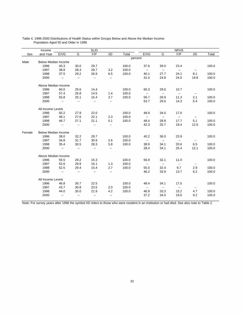
Table 4. 1996-2000 Distributions of Health Status within Groups Below and Above the Median Income: Population Aged 50 and Older in 1996
IncomeSex and Year E/VG G F/P I/D Total E/VG G F/P I/D Total
Male Below Median Income1996 40.3 30.0 29.7 100.0 37.6 39.0 23.4 100.01997 38.8 28.3 29.7 3.2 100.0 -- -- -- --1998 37.5 29.2 26.9 6.5 100.0 40.1 27.7 24.1 8.1 100.02000 -- -- -- -- 31.0 24.8 24.5 19.8 100.0
Above Median Income1996 60.0 25.6 14.4 100.0 60.3 29.0 10.7 100.01997 57.4 26.8 14.5 1.4 100.0 -- -- -- --1998 55.8 25.1 15.4 3.7 100.0 56.7 29.9 11.3 2.1 100.02000 -- -- -- -- 53.7 26.6 14.3 5.4 100.0
All Income Levels1996 50.2 27.8 22.0 100.0 48.9 34.0 17.0 100.01997 48.1 27.6 22.1 2.3 100.0 -- -- -- --1998 46.7 27.1 21.1 5.1 100.0 48.4 28.8 17.7 5.1 100.02000 -- -- -- -- 42.3 25.7 19.4 12.6 100.0
Female Below Median Income1996 38.0 32.2 29.7 100.0 40.2 36.0 23.9 100.01997 34.8 31.7 30.9 2.6 100.0 -- -- -- --1998 35.4 30.5 28.3 5.8 100.0 38.9 34.1 20.6 6.5 100.02000 -- -- -- -- 28.4 34.1 25.4 12.1 100.0
Above Median Income1996 55.5 29.2 15.3 100.0 56.9 32.1 11.0 100.01997 52.6 29.9 16.1 1.3 100.0 -- -- -- --1998 52.5 29.4 15.4 2.7 100.0 55.0 32.4 9.7 2.9 100.02000 -- -- -- -- 46.2 33.9 13.7 6.2 100.0
All Income Levels1996 46.8 30.7 22.5 100.0 48.4 34.1 17.5 100.01997 43.7 30.8 23.5 2.0 100.0 -- -- -- --1998 44.0 30.0 21.9 4.2 100.0 46.9 33.3 15.2 4.7 100.02000 -- -- -- -- 37.2 34.0 19.6 9.2 100.0
Note: For survey years after 1996 the symbol I/D refers to those who were resident in an institution or had died. See also note to Table 2.
32
SLID NPHS
percent

Table 5. 1996-2000 Distributions of Health Status within 'Low' and 'High' Education Groups: Population Aged 50 and Older in 1996
EducationSex and Year E/VG G F/P I/D Total E/VG G F/P I/D Total
Male 'Low' Education1996 44.2 29.3 26.5 100.0 41.8 35.7 22.5 100.01997 41.0 28.9 27.2 2.9 100.0 -- -- -- --1998 41.1 27.6 25.0 6.3 100.0 41.7 27.5 24.2 6.6 100.02000 -- -- -- -- 34.5 26.0 22.5 17.0 100.0
'High' Education1996 58.1 25.8 16.1 100.0 56.3 32.3 11.4 100.01997 57.4 25.8 15.4 1.5 100.0 -- -- -- --1998 54.0 26.5 16.0 3.5 100.0 55.2 30.2 11.1 3.6 100.02000 -- -- -- -- 50.3 25.4 16.2 8.1 100.0
All Education Levels1996 50.2 27.8 22.0 100.0 48.9 34.0 17.0 100.01997 48.1 27.6 22.1 2.3 100.0 -- -- -- --1998 46.7 27.1 21.1 5.1 100.0 48.4 28.8 17.7 5.1 100.02000 -- -- -- -- 42.3 25.7 19.4 12.6 100.0
Female 'Low' Education1996 40.4 33.0 26.6 100.0 40.1 37.3 22.5 100.01997 37.6 32.5 27.5 2.4 100.0 -- -- -- --1998 38.1 31.4 25.6 5.0 100.0 40.2 35.7 17.9 6.3 100.02000 -- -- -- -- 29.1 35.8 23.8 11.4 100.0
'High' Education1996 58.1 26.6 15.3 100.0 58.6 30.0 11.4 100.01997 54.7 27.7 16.4 1.3 100.0 -- -- -- --1998 54.4 27.4 15.3 2.9 100.0 55.1 30.3 11.9 2.8 100.02000 -- -- -- -- 47.2 31.9 14.5 6.5 100.0
All Education Levels1996 46.8 30.7 22.5 100.0 48.4 34.1 17.5 100.01997 43.7 30.8 23.5 2.0 100.0 -- -- -- --1998 44.0 30.0 21.9 4.2 100.0 46.9 33.3 15.2 4.7 100.02000 -- -- -- -- 37.2 34.0 19.6 9.2 100.0
Note: See note to Table 4.
33
SLID NPHS
percent

Table 6. 1996-2000 Distributions of Health Status within 'Young' and 'Old' Age Groups: Population Aged 50 and Older in 1996
AgeSex and Year E/VG G F/P I/D Total E/VG G F/P I/D Total
Male 'Old' (Ages 70+)1996 37.9 31.3 30.8 100.0 38.6 39.0 22.5 100.01997 34.2 30.9 29.4 5.5 100.0 -- -- -- --1998 30.6 30.5 26.4 12.6 100.0 35.8 25.8 24.8 13.6 100.02000 -- -- -- -- 24.4 20.6 23.2 31.8 100.0
'Young' (Ages 50-69)1996 54.8 26.5 18.7 100.0 52.7 32.3 15.1 100.01997 53.3 26.3 19.3 1.1 100.0 -- -- -- --1998 52.7 25.9 19.2 2.2 100.0 52.9 29.9 15.2 2.1 100.02000 -- -- -- -- 48.8 27.5 18.0 5.7 100.0
All Ages1996 50.2 27.8 22.0 100.0 48.9 34.0 17.0 100.01997 48.1 27.6 22.1 2.3 100.0 -- -- -- --1998 46.7 27.1 21.1 5.1 100.0 48.4 28.8 17.7 5.1 100.02000 -- -- -- -- 42.3 25.7 19.4 12.6 100.0
Female 'Old' (Ages 70+)1996 38.0 35.3 26.8 100.0 39.1 37.4 23.5 100.01997 34.3 33.6 27.8 4.4 100.0 -- -- -- --1998 32.3 32.2 26.1 9.5 100.0 35.2 36.1 18.2 10.5 100.02000 -- -- -- -- 22.8 32.5 24.3 20.5 100.0
'Young' (Ages 50-69)1996 51.6 28.3 20.2 100.0 53.0 32.4 14.6 100.01997 48.9 29.3 21.2 0.7 100.0 -- -- -- --1998 50.3 28.7 19.6 1.4 100.0 52.5 31.9 13.7 1.9 100.02000 -- -- -- -- 44.2 34.8 17.4 3.7 100.0
All Ages1996 46.8 30.7 22.5 100.0 48.4 34.1 17.5 100.01997 43.7 30.8 23.5 2.0 100.0 -- -- -- --1998 44.0 30.0 21.9 4.2 100.0 46.9 33.3 15.2 4.7 100.02000 -- -- -- -- 37.2 34.0 19.6 9.2 100.0
Note: See note to Table 4.
34
SLID NPHS
percent

Table 7. Probabilities of Remaining in Good Health and p-Value Test Statistics Based on Probit Regression Models
Male Female Male FemaleIndependent Variable ∆P p-value ∆P p-value ∆P p-value ∆P p-value
Income quartile: 1 -- -- -- -- -- -- -- --2 0.0303 0.060 0.0207 0.222 0.0289 0.602 0.0692 0.0543 0.0414 0.009 0.0488 0.004 0.1156 0.022 0.0334 0.3684 0.0770 0.000 0.0708 0.000 0.1609 0.002 0.1386 0.000
All income categories (Wald test) 0.000 0.000 0.006 0.002
Education: Less than grade 11 -0.0499 0.016 -0.0655 0.000 0.1120 0.119 0.0413 0.335 High school 11+ -- -- -- -- -- -- -- -- Some postsecondary 0.0070 0.721 0.0186 0.255 0.1078 0.137 0.0643 0.120 University degree 0.0507 0.025 0.0721 0.008 0.2026 0.007 0.1236 0.018 All education categories (Wald test) 0.000 0.000 0.047 0.081
Age group: 50-54 -- -- -- -- -- -- -- -- 55-59 -0.0839 0.001 -0.0700 0.004 0.0291 0.678 -0.0218 0.684 60-64 -0.0776 0.002 -0.0465 0.070 -0.0064 0.924 -0.0746 0.177 65-69 -0.1150 0.000 -0.0993 0.000 -0.1677 0.015 -0.1005 0.061 70-74 -0.1781 0.000 -0.0899 0.001 -0.1596 0.022 -0.1504 0.010 75-79 -0.2269 0.000 -0.2020 0.000 -0.4117 0.000 -0.2645 0.000 80-84 -0.3146 0.000 -0.2572 0.000 -0.4667 0.000 -0.3865 0.000 85+ -0.4194 0.000 -0.3871 0.000 -0.4945 0.000 -0.4415 0.000 All age categories (Wald test) 0.000 0.000 0.000 0.000
No. of observations 5992 7027 1431 1924Pseudo R-squared 0.0741 0.0775 0.1238 0.0900
Male Female Male FemaleIndependent Variable ∆P p-value ∆P p-value ∆P p-value ∆P p-value
Income quartile: 1 -- -- -- -- -- -- -- --2 0.0130 0.323 0.0323 0.011 0.0755 0.137 0.0090 0.5783 0.0217 0.084 0.0413 0.001 0.1008 0.043 0.0160 0.3464 0.0474 0.000 0.0590 0.000 0.1638 0.001 0.0417 0.003
All income categories (Wald test) 0.001 0.000 0.009 0.030
Education: Less than grade 11 -0.0304 0.060 -0.0472 0.003 0.0908 0.267 -0.0375 0.185 High school 11+ -- -- -- -- -- -- -- -- Some postsecondary 0.0026 0.864 0.0036 0.808 0.1401 0.068 -0.0180 0.485 University degree 0.0225 0.227 0.0541 0.013 0.1870 0.027 0.0081 0.789 All education categories (Wald test) 0.011 0.000 0.050 0.234
Age group: 50-54 -- -- -- -- -- -- -- -- 55-59 -0.0549 0.004 -0.0390 0.067 0.0803 0.279 -0.0110 0.655 60-64 -0.0682 0.001 -0.0276 0.220 0.0238 0.744 -0.0233 0.410 65-69 -0.0591 0.002 -0.0714 0.002 -0.1282 0.102 -0.0304 0.252 70-74 -0.1343 0.000 -0.0700 0.002 -0.1101 0.151 -0.0319 0.273 75-79 -0.1539 0.000 -0.1790 0.000 -0.3249 0.001 -0.1287 0.001 80-84 -0.1956 0.000 -0.1924 0.000 -0.3228 0.001 -0.1261 0.002 85+ -0.3626 0.000 -0.3634 0.000 -0.3967 0.010 -0.2472 0.000 All age categories (Wald test) 0.000 0.000 0.000 0.000
No. of observations 6092 7162 1431 1925Pseudo R-squared 0.0567 0.0800 0.1292 0.0683
35
Note: ∆P values are differential probabilities (differences from reference category probabilities). The p-value for an individual variable corresponds to a two-tailed test of the null hypothesis that the variable's coefficient is zero and is calculated using bootstrap weights provided by Statistics Canada. See Yeo et al. (1999) for details of the procedure.
SLID 1996, 1997 & 1998 NPHS 1996, 1998 & 2000
SLID 1996 & 1998 NPHS 1996 & 1998

Table A1. SLID OLS Regressions for ln(Y/LICO) Based on SLID Data
IndependentVariable Coefficient p-value Coefficient p-value Coefficient p-value Coefficient p-value
Constant 0.4745 0.446 -4.6595 0.000 0.5386 0.380 -4.5361 0.000Age group: 50-54 – – – – – – – – 55-59 -0.0776 0.022 -0.1169 0.005 -0.0660 0.054 -0.1244 0.002 60-64 -0.1941 0.000 -0.1780 0.000 -0.1846 0.000 -0.1880 0.000 65-69 -0.2024 0.000 -0.1012 0.002 -0.1966 0.000 -0.1110 0.001 70-74 -0.2477 0.000 -0.1139 0.001 -0.2405 0.000 -0.1174 0.000 75-79 -0.2837 0.000 -0.1649 0.000 -0.2720 0.000 -0.1676 0.000 80-84 -0.3885 0.000 -0.2110 0.000 -0.3753 0.000 -0.2127 0.000 85-89 -0.3028 0.001 -0.2468 0.000 -0.2799 0.003 -0.2391 0.000Edn: Less than gr. 11 -0.1942 0.000 -0.2637 0.000 -0.1807 0.000 -0.2620 0.000 High school 11 + – – – – – – – – Some postsec. 0.0198 0.505 0.0597 0.031 0.0348 0.270 0.0622 0.023 Univ. degree 0.3816 0.000 0.2767 0.000 0.3977 0.000 0.2835 0.000Marital Status: Single -0.5111 0.000 -0.2807 0.001 -0.5079 0.000 -0.3061 0.000 Married – – – – – – – – Separated -0.3524 0.000 -0.6460 0.000 -0.3342 0.000 -0.6395 0.000 Divorced -0.2699 0.000 -0.4905 0.000 -0.2701 0.000 -0.5029 0.000 Widowed -0.0818 0.134 -0.2715 0.000 -0.1198 0.069 -0.2788 0.000Immigrated: Not immigrant – – – – – – – – 0-10 yrs. ago -0.2676 0.352 -0.5653 0.000 -0.2763 0.323 -0.5582 0.000 11-14 yrs. ago -0.5341 0.000 -0.4509 0.000 -0.5409 0.000 -0.4577 0.000 15+ yrs. ago -0.0623 0.028 -0.0870 0.015 -0.0621 0.026 -0.0840 0.018Location: CMA – – – – – – – – CA 0.0393 0.137 0.1060 0.000 0.0376 0.154 0.1060 0.000
Other urban 0.0644 0.026 0.1641 0.000 0.0613 0.034 0.1599 0.000 Rural 0.1109 0.001 0.2976 0.000 0.1047 0.001 0.2951 0.000Province: NF -0.3326 0.000 -0.3513 0.000 -0.3306 0.000 -0.3541 0.000 PEI -0.2139 0.000 -0.1636 0.000 -0.2232 0.000 -0.1691 0.000 NS -0.1868 0.000 -0.2262 0.000 -0.1843 0.000 -0.2208 0.000 NB -0.1878 0.000 -0.2282 0.000 -0.1864 0.000 -0.2269 0.000 QC -0.2758 0.000 -0.2698 0.000 -0.2834 0.000 -0.2665 0.000 ON – – – – – – – – MB -0.2400 0.000 -0.2275 0.000 -0.2413 0.000 -0.2290 0.000 SK -0.1250 0.002 -0.0990 0.004 -0.1242 0.002 -0.1084 0.003 AB -0.1773 0.000 -0.1764 0.000 -0.1766 0.000 -0.1687 0.000 BC -0.1040 0.006 -0.1029 0.004 -0.1034 0.005 -0.0989 0.005ln(LICO) 0.0660 0.281 0.5741 0.000 0.0581 0.337 0.5622 0.000
No. of observations 5983 7015 6083 7149R-squared 0.2182 0.2770 0.2185 0.2789
36
Note: p-values correspond to two-tailed tests of the null hypothesis that a coefficient is zero. White's robust estimator of variance is used in all tests (White, 1980). Variables are defined in the text.
SLID 1996, 1997 & 1998 SLID 1996 & 1998Males Females Males Females

Table A2. OLS Regressions for ln(Y/LICO) Based on NPHS Data
IndependentVariable Coefficient p-value Coefficient p-value Coefficient p-value Coefficient p-value
Constant 4.7882 0.000 3.1751 0.009 4.7882 0.000 3.1751 0.009Age group: 50-54 – – – – – – – – 55-59 -0.0975 0.065 -0.2112 0.000 -0.0975 0.065 -0.2112 0.000 60-64 -0.2474 0.000 -0.2485 0.000 -0.2474 0.000 -0.2485 0.000 65-69 -0.3778 0.000 -0.2798 0.000 -0.3778 0.000 -0.2798 0.000 70-74 -0.3664 0.000 -0.3411 0.000 -0.3664 0.000 -0.3411 0.000 75-79 -0.5043 0.000 -0.3268 0.000 -0.5043 0.000 -0.3268 0.000 80-84 -0.5066 0.000 -0.3424 0.000 -0.5066 0.000 -0.3424 0.000 85-89 -0.1400 0.393 -0.3438 0.000 -0.1400 0.393 -0.3438 0.000Edn: Less than gr. 11 -0.2749 0.000 -0.1999 0.000 -0.2749 0.000 -0.1999 0.000 High school 11 + – – – – – – – – Some postsec. -0.0956 0.123 0.0551 0.241 -0.0956 0.123 0.0551 0.241 Univ. degree 0.1980 0.004 0.3712 0.000 0.1980 0.004 0.3712 0.000Marital Status: Single -0.2359 0.007 -0.3540 0.007 -0.2359 0.007 -0.3540 0.007 Married – – – – – – – – Separated -0.3593 0.000 -0.6126 0.000 -0.3593 0.000 -0.6126 0.000 Divorced -0.1134 0.227 -0.4822 0.000 -0.1134 0.227 -0.4822 0.000 Widowed -0.2131 0.005 -0.3728 0.000 -0.2131 0.005 -0.3728 0.000Immigrated: Not immigrant – – – – – – – – 0-10 yrs. ago -1.1957 0.000 -0.1275 0.596 -1.1957 0.000 -0.1275 0.596 11-14 yrs. ago -0.7438 0.000 -0.2680 0.039 -0.7438 0.000 -0.2680 0.039 15+ yrs. ago -0.1258 0.003 -0.0899 0.029 -0.1258 0.003 -0.0899 0.029Location: Urban – – – – – – – – Rural -0.0032 0.940 0.0521 0.255 -0.0032 0.940 0.0521 0.255Province: NF -0.3856 0.000 -0.2308 0.000 -0.3856 0.000 -0.2308 0.000 PEI -0.1400 0.034 -0.1862 0.006 -0.1400 0.034 -0.1862 0.006 NS -0.0973 0.111 -0.0746 0.249 -0.0973 0.111 -0.0746 0.249 NB -0.1678 0.005 -0.0686 0.216 -0.1678 0.005 -0.0686 0.216 QC -0.2163 0.000 -0.2045 0.000 -0.2163 0.000 -0.2045 0.000 ON – – – – – – – – MB -0.1796 0.009 -0.1761 0.000 -0.1796 0.009 -0.1761 0.000 SK -0.1899 0.003 -0.0899 0.125 -0.1899 0.003 -0.0899 0.125 AB -0.2206 0.004 -0.0638 0.281 -0.2206 0.004 -0.0638 0.279 BC -0.0343 0.506 -0.0891 0.079 -0.0343 0.506 -0.0891 0.079ln(LICO) -0.3674 0.001 -0.2248 0.063 -0.3674 0.001 -0.2248 0.063
No. of observations 1425 1920 1425 1921R-squared 0.3218 0.3163 0.3218 0.3164Note: See note to Table A1.
37
NPHS 1996, 1998 & 2000 NPHS 1996 & 1998Males Females Males Females

SEDAP RESEARCH PAPERS: Recent Releases
Number Title Author(s)
38
(2003)
No. 89: The Wealth and Asset Holdings of U.S.-Born and Foreign-Born Households: Evidence from SIPP Data
D.A. Cobb-ClarkV. Hildebrand
No. 90: Population Aging, Productivity, and Growth in LivingStandards
W. Scarth
No. 91: A Life-course Perspective on the Relationship between Socio-economic Status and Health: Testing the DivergenceHypothesis
S.G. Prus
No. 92: Immigrant Mental Health and Unemployment S. Kennedy
No. 93: The Relationship between Education and Health in Australiaand Canada
S. Kennedy
No. 94: The Transition from Good to Poor Health: An EconometricStudy of the Older Population
N.J. BuckleyF.T. DentonA.L. RobbB.G. Spencer
No. 95: Using Structural Equation Modeling to Understand the Role ofInformal and Formal Supports on the Well-being ofCaregivers of Persons with Dementia
P. RainaC. McIntyreB. ZhuI. McDowellL. SantaguidaB. KristjanssonA. HendricksL.W. Chambers
No. 96: Helping to Build and Rebuild Secure Lives and Futures: Intergenerational Financial Transfers from Parents to AdultChildren and Grandchildren
J. PloegL. CampbellM. DentonA. JoshiS. Davies
No. 97: Geographic Dimensions of Aging in Canada1991-2001
E.G. MooreM.A. Pacey
No. 98: Examining the “Healthy Immigrant Effect” in Later Life: Findings from the Canadian Community Health Survey
E.M. GeeK.M. KobayashiS.G. Prus
No. 99: The Evolution of High Incomes in Canada, 1920-2000 E. SaezM.R. Veall

SEDAP RESEARCH PAPERS: Recent Releases
Number Title Author(s)
39
No. 100: Macroeconomic Implications of Population Aging and PublicPensions
M. Souare
No. 101: How Do Parents Affect the Life Chances of Their Children asAdults? An Idiosyncratic Review
J. Ermisch
No. 102: Population Change and Economic Growth: The Long-TermOutlook
F.T. DentonB.G. Spencer
No. 103: Use of Medicines by Community Dwelling Elderly in Ontario P.J. BallantyneJ.A. MarshmanP.J. ClarkeJ.C. Victor
No. 104: The Economic Legacy of Divorced and Separated Women inOld Age
L. McDonaldA.L. Robb
No. 105: National Catastrophic Drug Insurance Revisited: Who WouldBenefit from Senator Kirby's Recommendations?
T.F. CrossleyP.V. Grootendorst M.R. Veall
No. 106: WAGES in CANADA: SCF, SLID, LFS and the SkillPremium
A.L RobbL. MageeJ.B. Burbidge
No. 107: A Synthetic Cohort Analysis of Canadian Housing Careers T.F. CrossleyY. Ostrovsky
No. 108: The Policy Challenges of Population Ageing A. Walker
No. 109: Social Transfers and Income Inequality in Old-age: A Multi-national Perspective
R.L. BrownS.G. Prus
No. 110: Organizational Change and the Health and Well-Being ofHome Care Workers
M. DentonI.U. ZeytinogluS. Davies
No. 111: Stasis Amidst Change: Canadian Pension Reform in an Ageof Retrenchment
D. BélandJ. Myles
No. 112: Socioeconomic Aspects of Healthy Aging: Estimates Basedon Two Major Surveys
N.J. BuckleyF.T. DentonA.L. RobbB.G. Spencer

SEDAP RESEARCH PAPERS: Recent Releases
Number Title Author(s)
40
No. 113: An Invitation to Multivariate Analysis: An Example Aboutthe Effect of Educational Attainment on MigrationPropensities in Japan
A. OtomoK-L. Liaw
(2004)
No. 114: The Politics of Protest Avoidance: Policy Windows, LaborMobilization, and Pension Reform in France
D. BélandP. Marnier
No. 115: The Impact of Differential Cost Sharing of Non-SteroidalAnti-Inflammatory Agents on the Use and Costs of AnalgesicDrugs
P.V. GrootendorstJ.K. MarshallA.M. HolbrookL.R. DolovichB.J. O’BrienA.R. Levy
No. 116: The Wealth of Mexican Americans D.A. Cobb-ClarkV. Hildebrand
No. 117: Precautionary Wealth and Portfolio Allocation: Evidence fromCanadian Microdata
S. Alan
No. 118: Financial Planning for Later Life: Subjective Understandingsof Catalysts and Constraints
C.L. KempC.J. RosenthalM. Denton
No. 119: The Effect of Health Changes and Long-term Health on theWork Activity of Older Canadians
D. Wing Han AuT.F. CrossleyM. Schellhorn
No. 120: Pension Reform and Financial Investment in the United Statesand Canada
D. Béland
No. 121: Exploring the Returns to Scale in Food Preparation(Baking Penny Buns at Home)
T.F. CrossleyY. Lu
No. 122: Life-cycle Asset Accumulation andAllocation in Canada
K. Milligan
No. 123: Healthy Aging at Older Ages: Are Income and EducationImportant?
N.J. BuckleyF.T. DentonA.L. RobbB.G. Spencer
(2005)

SEDAP RESEARCH PAPERS: Recent Releases
Number Title Author(s)
41
No. 124: Exploring the Use of a Nonparametrically GeneratedInstrumental Variable in the Estimation of a Linear ParametricEquation
F.T. Denton
No. 125: Borrowing Constraints, The Cost of Precautionary Saving, andUnemployment Insurance
T.F. CrossleyH.W. Low
No. 126: Entry Costs and Stock Market Participation Over the LifeCycle
S. Alan
No. 127: Income Inequality and Self-Rated Health Status: Evidencefrom the European Community Household Panel
V. HildebrandP. Van Kerm
No. 128: Where Have All The Home Care Workers Gone? M. DentonI.U. ZeytinogluS. DaviesD. Hunter
No. 129: Survey Results of the New Health Care Worker Study: Implications of Changing Employment Patterns
I.U. ZeytinogluM. DentonS. DaviesA. BaumannJ. BlytheA. Higgins
No. 130 Does One Size Fit All? The CPI and Canadian Seniors M. Brzozowski
No. 131 Unexploited Connections Between Intra- and Inter-temporalAllocation
T.F. CrossleyH.W. Low
No. 132 Grandparents Raising Grandchildren in Canada: A Profile ofSkipped Generation Families
E. Fuller-Thomson
No. 133 Measurement Errors in Recall Food Expenditure Data N. AhmedM. BrzozowskiT.F. Crossley
No. 134 The Effect of Health Changes and Long-term Health on theWork Activity of Older Canadians
D.W.H. AuT. F. CrossleyM.. Schellhorn
No. 135 Population Aging and the Macroeconomy: Explorations in theUse of Immigration as an Instrument of Control
F. T. DentonB. G. Spencer

SEDAP RESEARCH PAPERS: Recent Releases
Number Title Author(s)
42
No. 136 Users and Suppliers of Physician Services: A Tale of TwoPopulations
F.T. DentonA. GafniB.G. Spencer
No. 137 MEDS-D USERS’ MANUAL F.T. Denton C.H. Feaver B.G.. Spencer
No. 138 MEDS-E USERS’ MANUAL F.T. Denton C.H. Feaver B.G. Spencer
No. 139 Socioeconomic Influences on the Health of Older Canadians: Estimates Based on Two Longitudinal Surveys(Revised Version of No. 112)
N.J. BuckleyF.T. DentonA.L. RobbB.G. Spencer