snamp spatial team integration team...

5/1/14

1

SNAMP SPATIAL TEAM!Integration Team Meeting"

May 1 2014"

Spatial Team Members UC Merced

•! Qinghua Guo (PI)

•! Wenkai Li *

•! Hong Yu *

•! Jacob Flanagan *

•! Yanjun Su *

* augmented with other funds

UC Berkeley

•! Maggi Kelly (PI)

•! Stefania Di Tommaso

Past Members

•! Marek Jakubowski - graduated

•! Feng Zhao – former postdoc

•! Celia Garcia-Feced ** - former visiting student

•! Sam Blanchard ** - former staff

** Visitors/no cost to SNAMP

5/1/14

2

!"#$%&'"(&)*(+*,*-&*./012*((#03*4#.#05.#%64*07#"#8*$*"90:(;<*'90

Spatial Team IT Webinar Outline !"#$%&'()$*)$+ %% !"(%% ,-.*%

=*,';$*0#".0;4*(42*>00 1/!2*0?;'@*(0 ABCBB0D0ABCAB0E4*(42*>0;F09@*01%#6#,0'@#%9*(0;F09@*001357:0G"#,0(*%;(90 07#8820?*,,-00 0ABCAB0D0ABCHB0

E4*(42*>0;F09@*01357:0I2.#(0';$%;"*"9C0</!6G'#6;"J0';,,*'6;"J0'@#,,*"8*!0#".0!/(%(2!*!0

07#8820?*,,-0 0ABCHB0K0ABCLM0

NO*DP02"9(;./'6;"09;09@*0I2.#(09*'@"2Q/*0 R2"8@/#0S/;0 0ABCLM0K0ABCTM000

I2.#(0#,8;(29@$!0F;(0*U9(#'6"80F;(*!90%#(#$*9*(!0N9(**0@*28@9J0VWXJ0'#";%-0';4*(J0I5YJ0F/*,J0*9'&P0

R2"8@/#0S/;0 ABCTM0K0AACBB0

I2.#(0#,8;(29@$!0F;(0$#%%2"804*8*9#6;"09-%*!0 R2"8@/#0S/;0 AACBB0K0AACAM0Z!*0;F0I2.#(0%(;./'9!02"01357:02"9*8(#6;"0N>#9*(J0G!@*(J0

F;(*!90G(*J0#".0@*#,9@P007#8820?*,,-0 AACAM0K0AACLB0

I2.#(0I*!!;"!0I*#("*.00 07#8820?*,,-0 AACLB0KAACMB0=(#%D/%0#".0*4#,/#6;"0 1/!2*0?;'@*(0 AACMB0K0AHCBB0

!"#$%&'"(&)*(+*,*-&*./012*((#03*4#.#05.#%64*07#"#8*$*"90:(;<*'90

Webinar Outline •! Overview of the Spatial chapter of the SNAMP final

report - Maggi Kelly! •! Overview of the SNAMP Lidar component: justification,

collection, challenges and surprises -!Maggi Kelly •! (Re-) introduction to the Lidar technique -!Maggi Kelly •! Lidar algorithms for extracting forest parameters (tree

height, DBH, canopy cover, LAI, fuel, etc.) - Qinghua Guo

•! Lidar algorithms for mapping vegetation types - Qinghua Guo

•! Use of Lidar products in SNAMP integration (water, fisher, forest fire, and health) -!Maggi Kelly

•! Lidar Lessons Learned -!Maggi Kelly

5/1/14

3

!"#$%&'"(&)*(+*,*-&*./012*((#03*4#.#05.#%64*07#"#8*$*"90:(;<*'90



collection, challenges and surprises -!Maggi Kelly •! (Re-) introduction to the Lidar technique -!Maggi Kelly •! Lidar algorithms for extracting forest parameters (tree





!"#$%&'"(&)*(+*,*-&*./012*((#03*4#.#05.#%64*07#"#8*$*"90:(;<*'90

Spatial Team Chapter of SNAMP Final Report

/ %0)$1(23'4()%5 %6#$#%6*7'1-84()%

59/ %:#7*%6#$#%595 %;-6<=%>%;-?"$%6*$*'4()%#)2%=#)?-)?%59@ %A-*B2%6#$#%

@ %C*$"(27%@9/ %C#-)%;-2#1%D1(23'$7E%6FCG%6FCG%HIC%@95 %,(8(?1#8"-'%81(23'$7%@9@ %;-2#1%C*$1-'7 %%@9J %A(1*7$%7$13'$31*%81(23'$7%@9K %L*?*$#4()%C#87 %%

J %=*73B$7 %%J9/ %C#-)%;-2#1%D1(23'$7E%6FCG%6FCG%HIC%J95 %,(8(?1#8"-'%81(23'$7 %%J9@ %;-2#1%C*$1-'7 %%J9J %A(1*7$%7$13'$31*%81(23'$7 %%J9K %L*?*$#4()%C#87 %%

K %6-7'377-()0

M %=*7(31'*N78*'-O'%.#)#?*.*)$%-.8B-'#4()7%#)2%1*'(..*)2#4()7%

M9/ %H(.8#1-7()%P*$Q**)%B-2#1%#)2%(84'#B%-.#?*1R%M95 %;-2#1%'"#BB*)?*7%%M9@ %;-)S7%Q-$"%Q-B2B-T*%M9J %H(7$%(T%;-2#1 %%M9K %6#$#%'()7-2*1#4()7%Q-$"%;-2#1%

U %=*T*1*)'*7 %%V %<88*)2-'*7 %%

V9/ %<88*)2-W%<E%:#7*%X0F%6#$#%%V95 %<88*)2-W%:E%FY<CD%F8#4#B%,*#.%D3PB-'#4()7 %%V9@ %<88*)2-W%:E%F8#4#B%,*#.%Y*Q7B*Z*17 %%

%>%;-?"$%6*$*'4()%#)2%=#)?-)?%

%D1(23'$7E%6FCG%6FCG%HIC%,(8(?1#8"-'%81(23'$7%

A(1*7$%7$13'$31*%81(23'$7%L*?*$#4()%C#87

%D1(23'$7E%6FCG%6FCG%HIC%,(8(?1#8"-'%81(23'$7

A(1*7$%7$13'$31*%81(23'$7L*?*$#4()%C#87

M =*7(31'*N78*'-O'%.#)#?*.*)$%-.8B-'#4()7%#)2%1*'(..*)2#4()7%

M9/ H(.8#1-7()%P*$Q**)%(84'#B%-.#?*1R%M95 ;-2#1%'"#BB*)?*7M9@ ;-)S7%Q-$"%Q-B2B-T*%M9J H(7$%(T%;-2#1M9K 6#$#%'()7-2*1#4()7%Q-$"%

U =*T*1*)'*7V <88*)2-'*7

V9/ <88*)2-W%<E%:#7*%X0F%6#$#V95 <88*)2-W%:E%FY<CD%F8#4#B%,*#.%D3PB-'#4()7V9@ <88*)2-W%:E%F8#4#B%,*#.%Y*Q7B*Z*17

5/1/14

4

!"#$%&'"(&)*(+*,*-&*./012*((#03*4#.#05.#%64*07#"#8*$*"90:(;<*'90



collection, challenges and surprises -!Maggi Kelly •! (Re-) introduction to the Lidar technique – Maggi Kelly •! Lidar algorithms for extracting forest parameters (tree





Spat

ial S

calin

g in

the

Rese

arch

5/1/14

5

We are evaluating forest fuel treatment impact on fire, wildlife, water quality and quantity in a BACI design: Before, After, Control, Implementation

Spatial Scale •! Each team will perform their research at a specific

scale: •! Fire & Forest Health team works at the scale of the

individual tree, to the forest stand, to the fireshed… •! Wildlife teams work at the scale of the individual tree and its

environs to the scale of an animal s home range… •! Water team works at the scale of the watershed… •! Public Participation works at local and national scales.

•! Spatial models will be used to integrate across teams, and extrapolate results in a common spatial framework Sp

atia

l Sca

ling

in th

e Re

sear

ch

!"#$%&'"(&)*(+*,*-&*./012*((#03*4#.#05.#%64*07#"#8*$*"90:(;<*'90

Planning 2007 2006 2005

February 2005 MOU Signed by UC, USFS, USFWS & CA Resources Agency

March 2005 UCST & MOUP initiate planning process to develop SNAMP

April 15, 2005 SNAMP proposal completed

December 9, 2005 First SNAMP Public Meeting

January 20, 2006 Public Comment Website Launch

February – December 2006 SNAMP Workplan reviewed by MOUP, Public, & Peer Review ; Study Sites are chosen

January 16, 2007 Revised SNAMP Workplan Posted

July 2 & Nov. 11, 2006 SNAMP Public meetings with UCST & MOUP

Data Collection & Analysis Synthesis, Integration

Inception

2012 2011 2010 2009 2008 2007

Wildlife, Water, PPT data collection continues

Pre-treatment Data Collection

Pre-Treatment

LiDAR flight: Sugar Pine

Water & Fisher begin data collection; LiDAR flight: Last Chance; Owl Study Area expands to include Eldorado

Public Outreach & Mutual Learning

2013 2014

2012 2011

Wildlife, Water, PPT data

Treatment

Public Outreach & Mutual Learning

2015 +

......

Adaptive management adjustments to policy due to research findings will be discussed and implemented by USFS

Post-Treatment Reporting

Wildlife, Water, PPT data Wildlife, Water, PPT data ...... LiDAR flight: Sugar Pine

Data Collection & Analysis Data Collection & Analysis

Public Outreach & Mutual Learning Public Outreach & Mutual Learning

LiDAR flight: Last Chance

SNAMP Timeline

5/1/14

6

!"#$%&'"(&)*(+*,*-&*./012*((#03*4#.#05.#%64*07#"#8*$*"90:(;<*'90

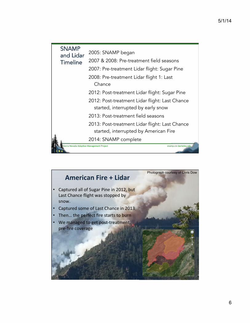
SNAMP and Lidar Timeline

2005: SNAMP began

2007 & 2008: Pre-treatment field seasons

2007: Pre-treatment Lidar flight: Sugar Pine

2008: Pre-treatment Lidar flight 1: Last Chance

2012: Post-treatment Lidar flight: Sugar Pine

2012: Post-treatment Lidar flight: Last Chance started, interrupted by early snow

2013: Post-treatment field seasons

2013: Post-treatment Lidar flight: Last Chance started, interrupted by American Fire

2014: SNAMP complete

!"#$%&'"(&)*(+*,*-&*./012*((#03*4#.#05.#%64*07#"#8*$*"90:(;<*'90

<.*1-'#)%A-1*%[%;-2#1%•! [#%9/(*.0#,,0;F01/8#(0:2"*02"0HBAHJ0)/90

I#!90[@#"'*0\28@90>#!0!9;%%*.0)-0!";>&00

•! [#%9/(*.0!;$*0;F0I#!90[@#"'*02"0HBAL0•! ]@*"^09@*0%*(F*'90G(*0!9#(9!09;0)/("0•! =*0$#"#8*.09;08*90%;!9D9(*#9$*"9J0

%(*DG(*0';4*(#8*0

Photograph courtesy of Chris Dow

5/1/14

7

!"#$%&'"(&)*(+*,*-&*./012*((#03*4#.#05.#%64*07#"#8*$*"90:(;<*'90

:;!9D9(*#9$*"9J0:(*DG(*0I2.#(05'Q/2!26;"0

2012 Flight 2013 Flight

5$*(2'#"0_2(*0:*(2$*9*(0

Pre-Treatment collection (117km2): •! Sept 2007 •! Cost: $77,000 Post-Treatment collection: •! Nov 2012 •! Cost: $77,000

Pre-Treatment collection (107km2): •! Sept 2008 •! Cost: $70,000 Post-Treatment collection: •! Nov 2012 •! Aug 2013 •! Cost: $70,000

SNAMP Lidar Information Common Discrete Lidar specs: 4 range measurements per pulse Scan frequency: 40-45 Hz Pulse rate frequency: 70-100 KHz Divergence angle: 0.25 mrad Flying height: 600-800 m Footprint: 15 to 20 cm Wavelength: 1064 nm 4-10 cm elevation accuracy Footprint size: ~20 cm Swath width: ~510 m ~10 points/m2 Acquisition cost: ~ $650/km2, $6.5/ha, $2.6/acre Contracted with National Center for Airborne Laser Mapping (NCALM;) All surveys used an Optech GEMINI Airborne Laser Terrain Mapper (ALTM) mounted in a twin-engine Cessna Skymaster.

Last Chance Area

Sugar Pine Area

specs:

5/1/14

8

!"#$%&'"(&)*(+*,*-&*./012*((#03*4#.#05.#%64*07#"#8*$*"90:(;<*'90








Optical Remote Sensing: the View from Overhead

^7EVY10000000000000000000000000000000000000000000000I#".!#900000000000000000000000000000000000E(9@;%@;9;8(#%@-&&&0&&A+$0 0 0 0000000000 0LB$0 0 0 0 0 0 0A$&&0

16

5/1/14

9

Optical Remote Sensing: the View from Overhead

•! [#";%-0';4*(0•! `*8*9#6;"0%(;./'6429-0

9@(;/8@06$*0•! :@*";,;8-0•! `28;(0#".0@*#,9@0•! `*8*9#6;"0%#a*("2"80

•! ^>29@0!-";%6'0#".0(*82;"#,0!'#,*0';4*(#8*0

17

!"#$%&'"(&)*(+*,*-&*./012*((#03*4#.#05.#%64*07#"#8*$*"90:(;<*'90

^W/90>29@0;%6'#,0(*$;9*0!*"!2"8J0>*0'#"b908*90$/'@0#);/909@*04*(6'#,0!9(/'9/(*02"0F;(*!9!^0

18

5/1/14

10

Introduction to Lidar

Image modified from Lefsky et al. 2004 with tree graphic from globalforestscience.org.

Lidar = Light Detection and Ranging

Range. The measurement of the speed which a pulse of light returns to a sensor is converted to elevation above sea level.

R = "(tc) •! R = range

•! t = time

•! c = speed of light

LiDAR = Light Detection And Ranging

20

5/1/14

11

Dis

cret

e Li

dar y

ield

s m

ultip

le re

turn

s

first returns

second returns

third returns

last returns

all returns

last returns

all returns

21

Waveform Lidar

Image source: Pirotti, F. (2011). Analysis of full-waveform LiDAR data for forestry applications: a review of investigations and methods. iForest-Biogeosciences and Forestry, 4(3), 100.

5/1/14

12

23

SNAMP Field Data

Height, DBH, Species, Vigor (class), Crown class, HTLCB; Shrub Species, % cover, Height; Fuel: 1-, 10-, 100-, 1000-hour fuels, Litter, Duff layer. Other: LAI, Canopy cover (tube sightings), Coarse woody debris, Ladder fuel measurements

Height, DBH, Species, Vigor (class), Crown class, HTLCB; Shrub Species, % cover, Height; Fuel: 1-, 10-, 100-, 1000-hour fuels, Litter, Duff layer. Other: LAI, Canopy

5/1/14

13

The lidar deliverable

The lidar deliverable

26

NCALM standard products Raw LIDAR data in LAS or ASCII format •! All returns, unfiltered X, Y, Z, •! Return intensity, •! Scan angle, and •! GPS time data

Filtered LIDAR X, Y, Z (LAS or ASCII) DEM & DSM

5/1/14

14

Digital Surface

Model

Digital Terrain

Model

Individual Trees

Lidar Data Products

DTM – Digital Terrain Model •! Elevation information about

bare-earth surface without the influence of vegetation or man-made features

Individual Trees

Canopy Height

Model

CHM – Canopy Height Model •! Height information about

vegetation features with elevation removed

DSM – Digital Surface Model •! Elevation information about all

features in the landscape, including vegetation, buildings and other structures

Individual Trees •! Isolated from the point cloud,

containing location, height, diameter

27

!"#$%&'"(&)*(+*,*-&*./012*((#03*4#.#05.#%64*07#"#8*$*"90:(;<*'90








5/1/14

15

DEM products for both sites DEM completed for both sites: Publication looking at methodology for DEM creation (Guo et al, 2010),

based on different algorithms, topography, lidar sampling, density, pixel size.

Guo, Q., W. Li, H. Yu, and O. Alvarez. 2010. Effects of Topographic Variability and Lidar Sampling Density on Several DEM Interpolation Methods. Photogrammetric Engineering & Remote Sensing 76:701-712.

1/8#(0:2"*0 I#!90[@#"'*0

29

Forest Attribute Estimation and Assessment

Lidar Product List (20m):

Mean Height

Max Height

Diameter at Breast Height (DBH)

Height to Live Canopy Base (HTLCB)

Canopy Cover

Leaf area index (LAI)

Individual trees

Tree density

Tree size classes

Canopy fuel

Biomass

Sugar Pine Last Chance Sugar Pine

5/1/14

16

Vegetation Analysis: Lidar Metrics

5th

50th

95th

List of lidar metrics Height:

minimum mean maximum standard deviation skewness kurtosis quadratic mean

Percentiles:

0.01, 0.05, 0.10…0.99

Total number of returns Maximum foliage profile density Point density:

0 - .5 m, 0.5 – 1m…55 - 60m

There are about 30-40 commonly used lidar metrics.

Vegetation return

Ground return

Laser pulses

Gap Fraction (GP) = nground / (nvegetation + nground)

LAIe = - cos( ) ! ln(GF) / k : zenith angle (scan angle) k: extinction coefficient (0.5)

Richardson et al., 2009

Some of these measures are inferred from regression, some are direct measurements, or calculations

5/1/14

17

!"#$%&'"(&)*(+*,*-&*./012*((#03*4#.#05.#%64*07#"#8*$*"90:(;<*'90








Data Used for Vegetation Mapping

Lidar data •! Lidar metric data: 0%, 1%, 5%,…,99%, 100% •! Canopy cover •! Tree height •! Topography data: DEM, Slope, Aspect

Aerial imagery - NAIP •! Band information: Green, Red, NIR band. •! Texture information: Mean, Standard

Deviation, Homogeneity, Contrast, Dissimilarity, Entropy, Second Moment.

Plot Data •! 377 and 408 circular plots (12.62 m radius) at

Sugar Pine site and Last Chance site, respectively.

Plot Data

Lidar data

Aerial imagery - NAIP

5/1/14

18

Vegetation Mapping Procedure

Pixel-based Vegetation Mapping Result

Vegetation group determination and accuracy assessment

•  Post-hoc analysis •  Permutation test

Vegeta4on Class Leaf Area Index

Basal Area

Lorrey Height

Canopy Cover Eleva4on Vegeta4on composi4on

m2/ m2 m2 / ha m % m Open Pine-‐oak

forest 1.9 11.4 12.2 14.7 1,614 open pine-‐oak forest

Pine-‐cedar forest 3.9 19.8 17.6 38.1 1,518 ponderosa pine, incense cedar dominated forest

Mature Mixed Conifer 4.4 47.3 25.3 66.8 1,578

white-‐fir/cedar/ponderosa pine -‐-‐ mature mixed conifer

Closed-‐canopy Mixed Conifer 4.1 68.0 32.4 74.6 1,632

white-‐fir/cedar/sugar pine tall -‐-‐ dense mixed conifer

Open True FirPine Forest

Cedar Forest

Young Mixed Conifer

Mature Mixed Conifer

Primary Axis (E=0.27)

Seco

ndar

y Ax

is (E

= 0

.20)

VegClassOpen True FirPine ForestCedar ForestYoung Mixed ConiferMature Mixed Conifer

Primary axis

Seco

ndar

y ax

is

Vegetation Class Open True Fir Pine Forest Cedar Forest Young Mixed Conifer Mature Mixed Conifer

5/1/14

19

Pixel-based Vegetation Mapping Results

Sugar Pine

Last Chance

Object-based Vegetation Mapping Result

Vegetation map segments: Sugar Pine Vegetation map segments: Sugar Pine

5/1/14

20

Vegetation Change Detection Procedure

Iterative threshold selection method (Fung & LeDrew, 1988) •! The threshold value of mean canopy difference ± n standard deviations was

iteratively selected to obtain candidate “change” areas.

•! The n value was increased with an increment of 0.1 at each step until it reached 2.0. The corresponding threshold of n which produced the highest change detection accuracy was used as the threshold to separate the changed and unchanged areas.

Treatment detection method •! The treatment attribute for each polygon was determined by the majority of the

treatment attribute of the pixels within it.

•! Polygons with an area smaller than 800 m2 were removed. Finally, the remained treated polygons were used to cut the treated pixels and obtain the pixel-based forest treatment detection result.

Vegetation Change Detection Results: Last Chance

•! Accuracy assessment •! We compared our lidar

forest treatment detection with field measurements.

•! Total Accuracy: 95.66%. •! Kappa Coefficient: 0.78.

Predicted results

Treated Untreated

Treated 33 12

Untreated 4 320

Treated (polygons from USFS) Changed (from Lidar) Unchanged

Fiel

d m

easu

red Treated Untreated Untreated Untreated

Treated 33 12 12

Untreated 4 320 320

5/1/14

21

!"#$%&'"(&)*(+*,*-&*./012*((#03*4#.#05.#%64*07#"#8*$*"90:(;<*'90








SNAMP Lidar Products and Cross-team Integration

Lidar Product List:

DEM

Mean Height

Max Height



Canopy Cover


Individual trees

Tree density

Tree size classes

Canopy fuel

Biomass

Canopy Cover

DEM

Mean Height

Max Height



Canopy Cover

FFEH: Fire behavior models (e.g. Farsite) Fmodels (e.g.

5/1/14

22

Lidar Product List:

DEM

Mean Height

Max Height



Canopy Cover


Individual trees

Tree density

Tree size classes

Canopy fuel

Biomass

Canopy Cover


FFEH: Fire behavior models (e.g. Farsite)

Water: Hydrological modeling (e.g. Ressys) modeling (e.g.

Mean Height

DEM models (e.g.

modeling (e.g.


Lidar Product List:

DEM

Mean Height

Max Height



Canopy Cover


Individual trees

Tree density

Tree size classes

Canopy fuel

Biomass

Canopy Cover Canopy Cover


Water: Hydrological modeling (e.g. Ressys)

Owl: nest tree characterization

Individual trees


5/1/14

23

Lidar Product List:

DEM

Mean Height

Max Height



Canopy Cover


Individual trees

Tree density

Tree size classes

Canopy fuel

Biomass

Canopy Cover Canopy Cover




Fisher: Species distribution modeling,

den tree characterization Individual trees

DEM

Mean Height

Max Height modeling (e.g.


Lidar Product List:

DEM

Mean Height

Max Height



Canopy Cover


Individual trees

Tree density

Tree size classes

Canopy fuel

Biomass




Fisher: Species distribution modeling,

den tree characterization

Public Participation: Maps

DEM

Mean Height

Max Height



Canopy Cover


Individual trees

Tree density

Tree size classes

Canopy fuel

Biomass


5/1/14

24

Spat

ial P

ublic

atio

ns

•! SNAMP PUB #4: Guo, et al. 2010. Effects of topographic variability and lidar sampling density on several DEM interpolation methods. PERS 76(6): 701–712.

•! SNAMP PUB #5: Garcia-Feced, et al. 2011. LiDAR as a tool to characterize wildlife habitat: California spotted owl nesting habitat as an example. JF 108(8): 436-443.

•! SNAMP PUB #6: Li, et al. 2012. A new method for segmenting individual trees from the lidar point cloud. PERS 78(1): 75-84.

•! SNAMP PUB #7: Blanchard, et al. 2011. Object-Based Image Analysis of Downed Logs in Disturbed Forested Landscapes using Lidar. RS 3: 2420-2439. Spatial Team.

•! SNAMP PUB #13: Jakubowski, et al. 2013. Predicting surface fuel models and fuel metrics using lidar and CIR imagery in a dense, mountainous forest. PERS. 79(1): 37-49.

•! SNAMP PUB #14: Zhao, et al. 2012. Allometric equation choice impacts lidar-based forest biomass estimates: A case study from the Sierra National Forest, CA. AFM 165: 64– 72.

•! SNAMP PUB #16: Zhao, et al. 2012. Characterizing habitats associated with fisher den structures in southern Sierra Nevada forests using discrete return lidar. FEM. 280: 112–119.

•! SNAMP PUB #18: Jakubowski, Guo, and Kelly. 2013. Tradeoffs between lidar pulse density and forest measurement accuracy. RSE 130: 245–253.

•! SNAMP PUB #24: Jakubowski, M. J., W. Li, Q. Guo, and M. Kelly. 2013. Delineating individual trees from lidar data: a comparison of vector- and raster-based segmentation approaches. RS, 5: 4163-4186.

The focus of SNAMP Integration is through the vegetation maps the vegetation maps

Sugar Pine

Last Chance

5/1/14

25

!"#$%&'"(&)*(+*,*-&*./012*((#03*4#.#05.#%64*07#"#8*$*"90:(;<*'90

_,;>0;F02"9*8(#6;"0%(;./'9!0)*9>**"09*#$!0Plot field data from

FFEH

Raw lidar data from NCALM

NAIP imagery

from USDA

Processed lidar data

To Spatial To Spatial To Spatial

To Spatial and FFEH

Lidar-derived

vegetation map

Vegetation polygon map with up-scaled

plot data

To FFEH Fire modeling

based on vegetation

map

Spatially explicit

vegetation metrics from fire model

To Wildlife

To Water

To FFEH

Water integration

metrics

Fisher and Owl

integration metrics

Forest Ecosystem

Health integration

metrics

Integrated, multi-resource

assessment

!"#$%&'"(&)*(+*,*-&*./012*((#03*4#.#05.#%64*07#"#8*$*"90:(;<*'90








5/1/14

26

!"#$%&'"(&)*(+*,*-&*./012*((#03*4#.#05.#%64*07#"#8*$*"90:(;<*'90

SNAMP Lidar Lessons Learned

1.! Lidar is great for mapping forest structure. But what about if you don’t have it? Or need to work back in time?

2.! There are challenges with Lidar, especially discrete lidar –! understory

3.! Links with wildlife –! Lidar captures structure, but what do metrics mean in terms of

field data? –! What is a proxy for important structure that can be measured in

the field?

4.! Cost of Lidar: cost of acquisition, cost of analysis. 5.! Density of points, what is needed? 6.! Lidar data can get very large.

Point 1: Forest Attribute Estimation and Assessment Product Lidar Moderate-res

optical (Landsat)

High-res optical (NAIP)

Mean height * Max height *

DBH * * Height to live canopy

base *

Canopy cover Individual trees

Leaf area index (LAI) Tree density Canopy fuel

Biomass *

works works with reservations not possible

* from regression

5/1/14

27

Measuring fire-related forest structure with lidar

Results 1.! fuel types – shrub,

timber-litter, timber-understory - can be predicted reliably using lidar, but

2.! specific surface fuel

models are difficult to predict, and

3.! accuracy of continuous

canopy metrics decreases with lidar penetration into the canopy

Jakubowski, M. K., Q. Guo, B. Collins, S. Stephens, and M. Kelly. 2013. Predicting surface fuel models and fuel metrics using lidar and CIR imagery in a dense, mountainous forest. Photogrammetric Engineering and Remote Sensing 79(1):37-49

Viewing a Virtual Scene in 3D

Point 2: Understory is challenging

SNAMP Waveform Lidar

Waveform lidar might help us with understory, and also with wildlife metrics

Northern site lidar footprint

2012 lidar coverage – discrete + waveform

2008 lidar coverage – discrete return

Image source: Pirotti, F. (2011). Analysis of full-waveform LiDAR data for forestry applications: a review of investigations and methods. iForest-Biogeosciences and Forestry, 4(3), 100.

5/1/14

28

Point 3: Links with wildlife

–! Lidar captures structure, but what do metrics mean in terms of field data?

–! What is a proxy for important structure that can be measured in the field?

5th

50th

95th

We get good correlation between lidar metrics on structure and wildlife presence (e.g. Fisher den trees), but what does this mean for managers? What can a manager “see” and aim for in the forest? What does it mean that we get a statistical relationship between “kurtosis of heights” and fisher den trees? We need a better field and lidar derived proxy variable for structure.

Point 4: Lidar vs other imagery costs

•! Two published studies present costs: –! Wulder et al. (2008) estimated a cost of $3/ha (~$1.2/acre) for

mapping with low density (1pl/m2) discrete Lidar data. –! Wynne (2006) estimated lidar collection, field collection and

analysis would cost $83/acre ($34/ha).

•! SNAMP: –! ~10pt/m2 => $6/ha, $650/km2, $2.5/acre

•! Let’s compare with Landsat: –! In the 1980s Landsat cost $2 - $3/ha to create vegetation maps

(adjusted to 2000 dollars) –! In 2000, Landsat cost $0.30-$0.40/ha to create vegetation maps:

Franklin et al. (2000).

5/1/14

29

Lidar pulse density

depending on flying height, discrete return

lidar can yield pulse densities of 1-12

pulses/m2.

Point 5: How much is enough?

How much is enough? How dense does lidar data have to be for management goals? Or what happens when your site burns before you complete lidar acquisition?

Point 5: How much is enough?

5/1/14

30

From: Jakubowski, et al. 2013. Tradeoffs between lidar pulse density and forest measurement accuracy. Remote Sensing of Environment.

Accuracy is fairly consistent between 1 and 10 pulse/m2, for plot-scale forest metrics

Point 6: How do we represent a forest stand?

Forest Stand size: 5 ha (12.35 acres) Optical Imagery: Landsat TM (30m): 55 pixels (330 bytes) Landsat ETM (15m)*: 222 pixels (1.3 kb) SPOT (10m): 500 pixels (2 Kb) IKONOS (1m): 50,000 pixels (390 Kb)

Lidar Data: Lidar (1pl/m2) (4 returns): 200,000 points (5Mb)** Lidar (10 pl/m2) (4 returns): 2,000,000 points (50Mb)**

Details of forest stand coverage from a number of typical remote sensing sources, modified from Wulder et al. (2012).

* panchromatic or pan-sharpened. ** Lidar file sizes are approximate, and vary with compression format.

(330 bytes)

2,000,000 points (50Mb)**

Details of forest stand coverage from a number of typical remote sensing

** Lidar file sizes are approximate, and vary with compression format.

5/1/14

31

!"#$%&'"(&)*(+*,*-&*./012*((#03*4#.#05.#%64*07#"#8*$*"90:(;<*'90

SNAMP data availability and website curation

We will transfer immediately all the spatial data to the USFS server after the completion of project, and our spatial server (snamp.ucmerced.edu) will be maintained for one more year after the project finishes.

!"#$%&'"(&)*(+*,*-&*./012*((#03*4#.#05.#%64*07#"#8*$*"90:(;<*'90

Spatial Team IT Webinar Outline !"#$%&'()$*)$+ %% !"(%% ,-.*%

=*,';$*0#".0;4*(42*>00 1/!2*0?;'@*(0 ABCBB0D0ABCAB0E4*(42*>0;F09@*01%#6#,0'@#%9*(0;F09@*001357:0G"#,0(*%;(90 07#8820?*,,-00 0ABCAB0D0ABCHB0

E4*(42*>0;F09@*01357:0I2.#(0';$%;"*"9C0</!6G'#6;"J0';,,*'6;"J0'@#,,*"8*!0#".0!/(%(2!*!0

07#8820?*,,-0 0ABCHB0K0ABCLM0

NO*DP02"9(;./'6;"09;09@*0I2.#(09*'@"2Q/*0 R2"8@/#0S/;0 0ABCLM0K0ABCTM000

I2.#(0#,8;(29@$!0F;(0*U9(#'6"80F;(*!90%#(#$*9*(!0N9(**0@*28@9J0VWXJ0'#";%-0';4*(J0I5YJ0F/*,J0*9'&P0

R2"8@/#0S/;0 ABCTM0K0AACBB0

I2.#(0#,8;(29@$!0F;(0$#%%2"804*8*9#6;"09-%*!0 R2"8@/#0S/;0 AACBB0K0AACAM0Z!*0;F0I2.#(0%(;./'9!02"01357:02"9*8(#6;"0N>#9*(J0G!@*(J0

F;(*!90G(*J0#".0@*#,9@P007#8820?*,,-0 AACAM0K0AACLB0

I2.#(0I*!!;"!0I*#("*.00 07#8820?*,,-0 AACLB0KAACMB0=(#%D/%0#".0*4#,/#6;"0 1/!2*0?;'@*(0 AACMB0K0AHCBB0

5/1/14

32

!"#$%&'"(&)*(+*,*-&*./012*((#03*4#.#05.#%64*07#"#8*$*"90:(;<*'90

Upcoming SNAMP events

May 15, 2014 - Fire and Forest Health Integration Team meeting, McClellan May 30, 2014 - CAM/facilitation workshop, Marysville/Oregon House June 19, 2014 - American Fire field trip, Foresthill/Last Chance June 20, 2014 - CA Spotted Owl Integration Team meeting, Davis June 25, 2014 - CAM/facilitation workshop, Marysville/Oregon House July 31, 2014 - Pacific Fisher Integration Team meeting, Fresno September 4, 2014 - Water Integration Team meeting, Merced November 6, 2014 - final SNAMP Annual meeting, McClellan

More information at http://snamp.cnr.berkeley.edu

snamp spatial team integration team...

Documents