smith meter microloadinfo.smithmeter.com/literature/docs/tp06005.pdfvolume correction for...

The Most Trusted Name In Measurement

Calculations

Electronic Preset Delivery System

Smith Meter ® microLoad.net™

Issue/Rev. 0.2 (3/11) Bulletin TP06005

• TP06005 Issue/Rev. 0.2 (3/11)

CautionThe default or operating values used in this manual and in the program of the microLoad.net are for factory testing only and should not be construed as default or operating values for your metering system. Each metering system is unique and each program parameter must be reviewed and programmed for that specific metering system application.

DisclaimerFMC Technologies Measurement Solutions, Inc. hereby disclaims any and all responsibility for damages, including but not limited to consequential damages, arising out of or related to the inputting of incorrect or improper program or default values entered in connection with the microLoad.net.

ii

Issue/Rev. 0.2 (3/11) TP06005 •

Section I – Volume Calculations ............................................................................................................................ 1 Volume Calculations ..............................................................................................................................................1 Volume Calculations for Indicated Volume ........................................................................................................1 Volume Calculations for Gross ..........................................................................................................................1 Volume Calculations for Gross @ Standard Temperature (GST) .....................................................................1 Volume Calculations for Gross Standard Volume (GSV) ...................................................................................1

Section II – Mass Calculations ...............................................................................................................................2 Mass Calculations .................................................................................................................................................2

Section III – Meter Factor Linearization Calculations ..........................................................................................4 Meter Factor Linearization Calculations ................................................................................................................4

Section IV – Temperature Calculations ..................................................................................................................7 Volume Correction for Temperature (CTL) Calculation ..........................................................................................7 Volume Correction Factor Calculation Options ................................................................................................11 RTD Temperature Input Conversion ................................................................................................................13

Section V – Pressure Calculations .......................................................................................................................14 Volume Correction for Pressure (CPL) Calculation .............................................................................................14 Vapor Pressure Calculations ...........................................................................................................................16

Section VI – Load Average Calculations .............................................................................................................17 Load Average Values...........................................................................................................................................17

Section VII – Auto Prove Meter Factor Calculations ...........................................................................................18 Auto Prove Calculation ........................................................................................................................................18 CTSP (Correction for Temperature on Steel of a Prover) ................................................................................18 CTLP (Correction for Temperature on Liquid in a Prover) ...............................................................................18 Combined Correction Factor (CCF) For a Prover ............................................................................................18 Corrected Prover Volume ................................................................................................................................18 Corrected Meter Volume ..................................................................................................................................19 Meter Factor ....................................................................................................................................................19 Average Meter Factor ......................................................................................................................................19

Table of Contents

iii

• TP06005 Issue/Rev. 0.2 (3/11)iv

(This page intentionally left blank)

Issue/Rev. 0.2 (3/11) TP06005 • Page 1

Section I – Volume Calculations

Volume Calculations

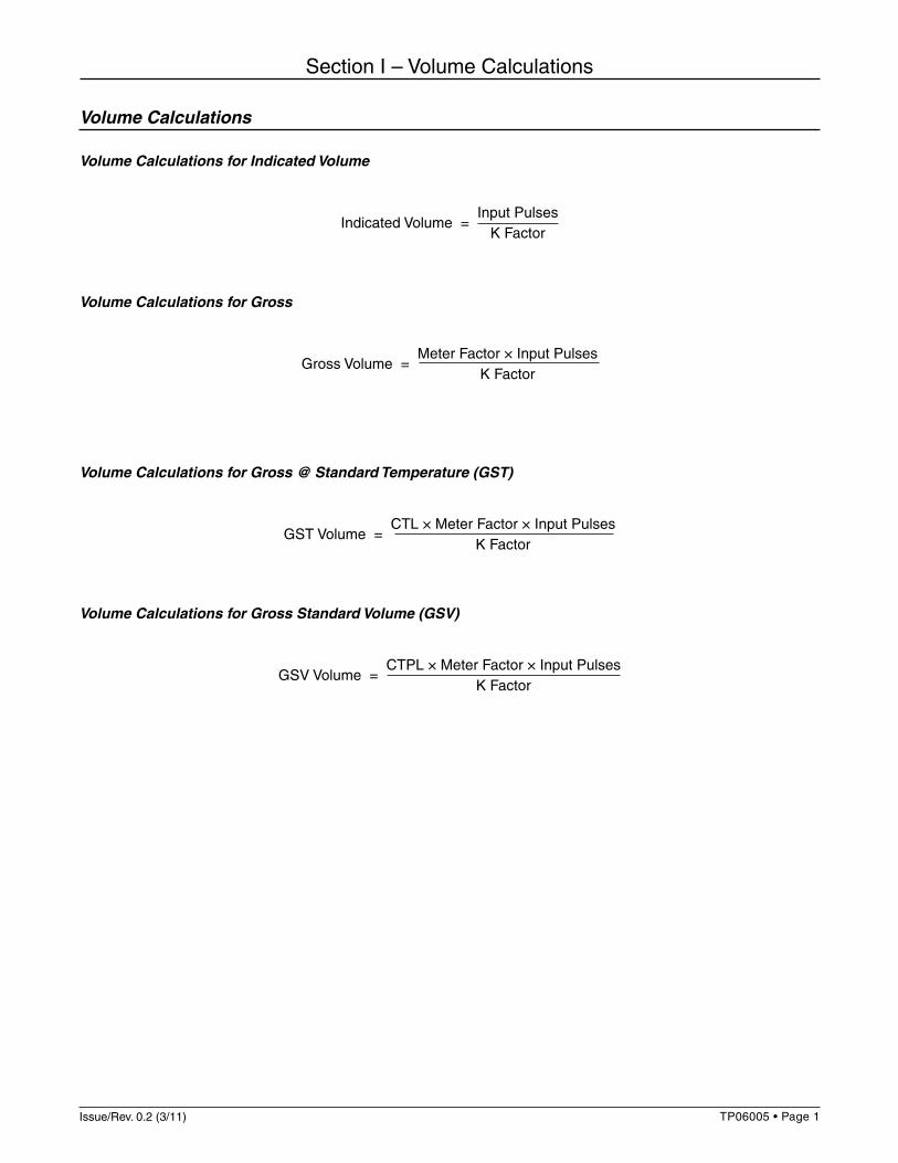
Volume Calculations for Indicated Volume

Indicated Volume = Input Pulses= K Factor

Volume Calculations for Gross

Gross Volume = Meter Factor × Input Pulses

K Factor

Volume Calculations for Gross @ Standard Temperature (GST)

GST Volume = CTL × Meter Factor × Input Pulses

K Factor

Volume Calculations for Gross Standard Volume (GSV)

GSV Volume = CTPL × Meter Factor × Input Pulses

K Factor

• TP06005 Issue/Rev. 0.2 (3/11)

Section II – Mass Calculations

Mass Calculations

A. Mass = Gross Volume × Observed Density

or

Mass = GSV × Reference Density

B. Mass calculation using reference density

1. Program entry conditions

a. A non-zero reference density entry.

b. Valid density units select entry.

c. Valid entries for GST compensation.

d. Mass units

2. Hardware conditions

a. A temperature probe installed. (Note: Maintenance temperature may be used instead of a temperature probe.)

3. Definition

With this method the reference density and GST volume are used to calculate the mass. Therefore, the reference density program code must contain a non-zero entry, temperature must be installed, and GST compensation must be available.

4. Calculation method

Mass = GST Volume × Reference Density

C. Mass calculation using a Densitometer

1. Program entry conditions

a. Valid density units select entry.

b. Valid densitometer configuration entries.

c. Mass units.

Issue/Rev. 0.2 (3/11) TP06005 • Page 3

Section II – Mass Calculations

2. Hardware conditions

a. A densitometer installed.

3. Definition

This method uses the densitometer input as the line density for calculating mass totals.

4. Calculation method

Mass = Gross Volume × Observed Density

Density CalculationThe density values derived from the API calculations are “in vacuo” values. If live density is used, the reference density calculated is “in vacuo.” Also, if a reference density for a fluid is entered into the AccuLoad (even tables), it should be an “in vacuo” value. If mass is calculated by the AccuLoad using the reference density and volume, the mass would also be “in vacuo.”According to API ASTM D 1250-04, pure fluid densities used in the calibration of densitometers are based on “weight in vacuo” and the readings obtained from such calibrations are also “in vacuo” values. The standard also states that all densities used in the API standard are “in vacuo” values.

• TP06005 Issue/Rev. 0.2 (3/11)

Section III – Meter Factor Linearization Calculations

Meter Factor Linearization CalculationsThe non-linearity of the meter calibration curve for each product can be approximated through use of a linearization method by entering meter factors at up to four different flow rates.The meter factors used will be determined from a straight line interpolation of the meter factor and its associated flow rate.

Graphically, the linearization method used can be represented as a point slope function between points:

Figure 1. Meter Factor vs. Flow Rate

where: MF1, MF2, MF3, MF4 = meter factors 1, 2, 3, and 4 Q1, Q2, Q3, Q4 = associated flow rates 1, 2, 3, and 4

The number of factors used is determined by the programming. Up to four factors are available at corresponding flow rates. (See the meter factors and flow rate program codes.)

The input meter pulses may also be monitored by the unit to verify the integrity of the meters and/or transmitters. This is accomplished through pulse comparator circuitry. The pulse comparator verifies the integrity of the meter and the voltage sense verifies the integrity of the transmitter. The type and resolution of the pulse input stream to the unit is also programmable.

The input resolution, pulse and transmitter integrity, meter factors and their controls and adjustments may be defined through use of program parameters.

Meter Factor Linearization

MF1

MF2

MF3

MF4

Q4 Q3 Q2 Q1

Issue/Rev. 0.2 (3/11) TP06005 • Page 5


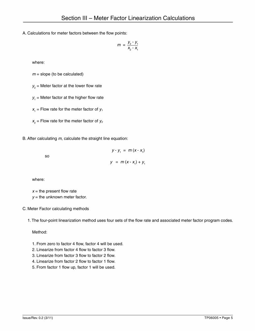
A. Calculations for meter factors between the flow points:

m = y2 - y1

x2 - x1

where:

m = slope (to be calculated)

y2 = Meter factor at the lower flow rate

y1 = Meter factor at the higher flow rate

x1 = Flow rate for the meter factor of y1

x2 = Flow rate for the meter factor of y2

B. After calculating m, calculate the straight line equation:

y - y1 = m (x - x1) so

y = m (x - x1) + y1

where:

x = the present flow rate y = the unknown meter factor.

C. Meter Factor calculating methods

1. The four-point linearization method uses four sets of the flow rate and associated meter factor program codes.

Method:

1. From zero to factor 4 flow, factor 4 will be used. 2. Linearize from factor 4 flow to factor 3 flow. 3. Linearize from factor 3 flow to factor 2 flow. 4. Linearize from factor 2 flow to factor 1 flow. 5. From factor 1 flow up, factor 1 will be used.

• TP06005 Issue/Rev. 0.2 (3/11)


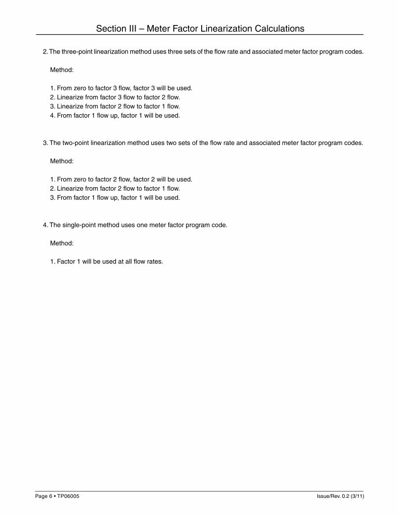
2. The three-point linearization method uses three sets of the flow rate and associated meter factor program codes.

Method:

1. From zero to factor 3 flow, factor 3 will be used. 2. Linearize from factor 3 flow to factor 2 flow. 3. Linearize from factor 2 flow to factor 1 flow. 4. From factor 1 flow up, factor 1 will be used.

3. The two-point linearization method uses two sets of the flow rate and associated meter factor program codes.

Method:

1. From zero to factor 2 flow, factor 2 will be used. 2. Linearize from factor 2 flow to factor 1 flow. 3. From factor 1 flow up, factor 1 will be used.

4. The single-point method uses one meter factor program code.

Method:

1. Factor 1 will be used at all flow rates.

Issue/Rev. 0.2 (3/11) TP06005 • Page 7

Section IV – Temperature Calculations

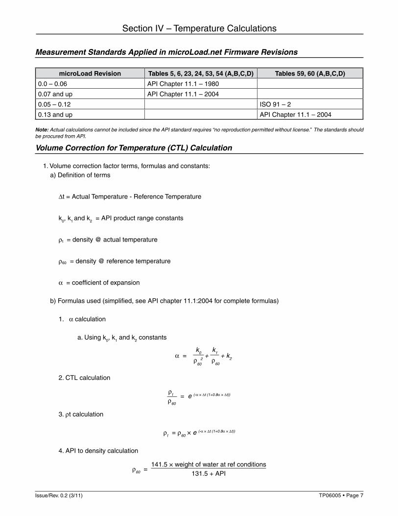
Measurement Standards Applied in microLoad.net Firmware Revisions

microLoad Revision Tables 5, 6, 23, 24, 53, 54 (A,B,C,D) Tables 59, 60 (A,B,C,D)

0.0 – 0.06 API Chapter 11.1 – 1980

0.07 and up API Chapter 11.1 – 2004

0.05 – 0.12 ISO 91 – 2

0.13 and up API Chapter 11.1 – 2004

Note: Actual calculations cannot be included since the API standard requires “no reproduction permitted without license.” The standards shouldbe procured from API.

Volume Correction for Temperature (CTL) Calculation

1. Volume correction factor terms, formulas and constants: a) Definition of terms

∆t = Actual Temperature - Reference Temperature

k0, k1 and k2 = API product range constants

ρt = density @ actual temperature

ρ60 = density @ reference temperature

α = coefficient of expansion

b) Formulas used (simplified, see API chapter 11.1:2004 for complete formulas)

1. α calculation

a. Using k0, k1 and k2 constants

α = k0 +

k1 + k2ρ 2 ρ60 60

2. CTL calculation

ρt = e (-α × ∆t (1+0.8α × ∆t))

ρ60 3. ρt calculation

ρt = ρ60 × e (-α × ∆t (1+0.8α × ∆t))

4. API to density calculation

ρ60 = 141.5 × weight of water at ref conditions

131.5 + API

• TP06005 Issue/Rev. 0.2 (3/11)


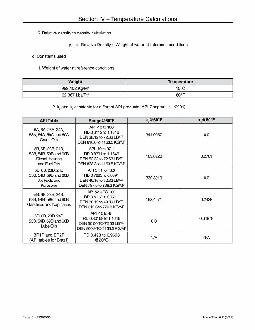
5. Relative density to density calculation

ρ60 = Relative Density × Weight of water at reference conditions

c) Constants used

1. Weight of water at reference conditions

Weight Temperature

999.102 Kg/M3 15°C

62.367 Lbs/Ft3 60°F

2. k0 and k1 constants for different API products (API Chapter 11.1:2004)

API Table Range@60°F k0@60°F k1@60°F

5A, 6A, 23A, 24A,53A, 54A, 59A and 60A

Crude Oils

API -10 to 100RD 0.6112 to 1.1646

DEN 38.12 to 72.63 LB/F3

DEN 610.6 to 1163.5 KG/M3

341.0957 0.0

5B, 6B, 23B, 24B,53B, 54B, 59B and 60B

Diesel, Heating and Fuel Oils

API -10 to 37.1RD 0.8391 to 1.1646

DEN 52.33 to 72.63 LB/F3

DEN 838.3 to 1163.5 KG/M3

103.8720 0.2701

5B, 6B, 23B, 24B53B, 54B, 59B and 60B

Jet Fuels and Kerosene

API 37.1 to 48.0RD 0.7883 to 0.8391

DEN 49.16 to 52.33 LB/F3

DEN 787.5 to 838.3 KG/M3

330.3010 0.0

5B, 6B, 23B, 24B,53B, 54B, 59B and 60B

Gasolines and Napthanes

API 52.0 TO 100RD 0.6112 to 0.7711

DEN 38.12 to 48.09 LB/F3

DEN 610.6 to 770.3 KG/M3

192.4571 0.2438

5D, 6D, 23D, 24D 53D, 54D, 59D and 60D

Lube Oils

API -10 to 45RD 0.80168 to 1.1646

DEN 50.00 TO 72.63 LB/F3

DEN 800.9 TO 1163.5 KG/M3

0.00.34878

BR1P and BR2P(API tables for Brazil)

RD 0.498 to 0.9693@20°C

N/A N/A

Issue/Rev. 0.2 (3/11) TP06005 • Page 9


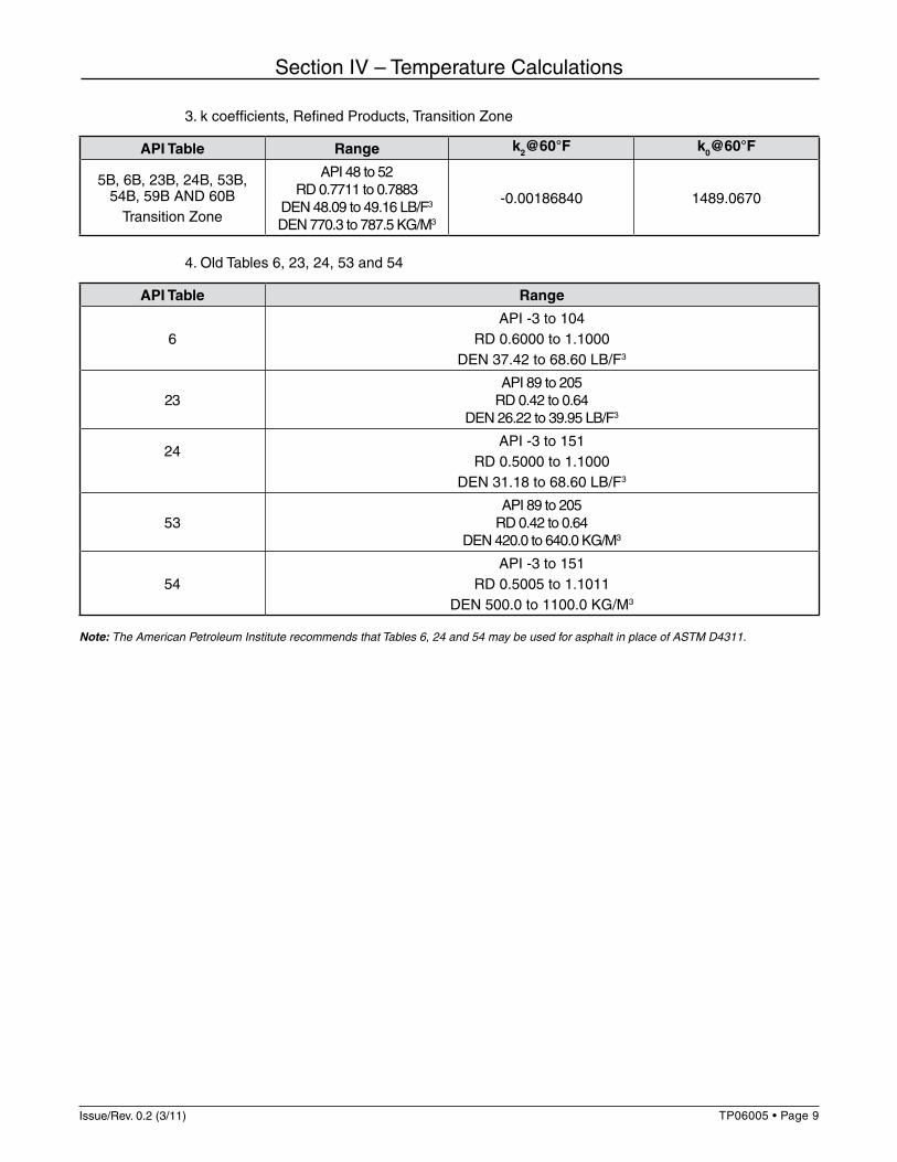
3. k coefficients, Refined Products, Transition Zone

API Table Range k2@60°F k0@60°F

5B, 6B, 23B, 24B, 53B, 54B, 59B AND 60B

Transition Zone

API 48 to 52RD 0.7711 to 0.7883

DEN 48.09 to 49.16 LB/F3

DEN 770.3 to 787.5 KG/M3

-0.00186840 1489.0670

4. Old Tables 6, 23, 24, 53 and 54

API Table Range

6API -3 to 104

RD 0.6000 to 1.1000DEN 37.42 to 68.60 LB/F3

23API 89 to 205

RD 0.42 to 0.64DEN 26.22 to 39.95 LB/F3

24API -3 to 151

RD 0.5000 to 1.1000DEN 31.18 to 68.60 LB/F3

53API 89 to 205

RD 0.42 to 0.64DEN 420.0 to 640.0 KG/M3

54API -3 to 151

RD 0.5005 to 1.1011DEN 500.0 to 1100.0 KG/M3

Note: The American Petroleum Institute recommends that Tables 6, 24 and 54 may be used for asphalt in place of ASTM D4311.

• TP06005 Issue/Rev. 0.2 (3/11)


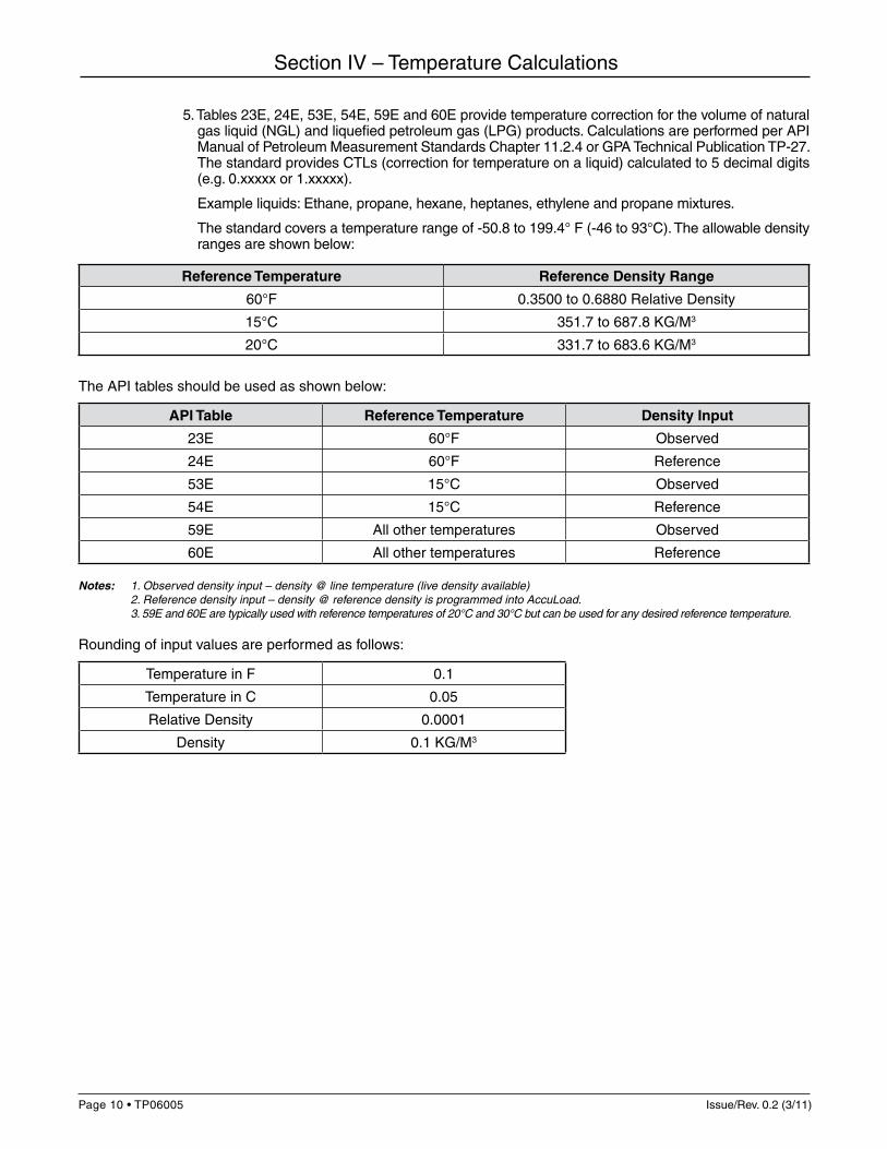
5. Tables 23E, 24E, 53E, 54E, 59E and 60E provide temperature correction for the volume of natural gas liquid (NGL) and liquefied petroleum gas (LPG) products. Calculations are performed per API Manual of Petroleum Measurement Standards Chapter 11.2.4 or GPA Technical Publication TP-27. The standard provides CTLs (correction for temperature on a liquid) calculated to 5 decimal digits (e.g. 0.xxxxx or 1.xxxxx).

Example liquids: Ethane, propane, hexane, heptanes, ethylene and propane mixtures.

The standard covers a temperature range of -50.8 to 199.4° F (-46 to 93°C). The allowable density ranges are shown below:

Reference Temperature Reference Density Range

60°F 0.3500 to 0.6880 Relative Density

15°C 351.7 to 687.8 KG/M3

20°C 331.7 to 683.6 KG/M3

The API tables should be used as shown below:

API Table Reference Temperature Density Input

23E 60°F Observed

24E 60°F Reference

53E 15°C Observed

54E 15°C Reference

59E All other temperatures Observed

60E All other temperatures Reference

Notes: 1. Observed density input – density @ line temperature (live density available) 2. Reference density input – density @ reference density is programmed into AccuLoad. 3. 59E and 60E are typically used with reference temperatures of 20°C and 30°C but can be used for any desired reference temperature.

Rounding of input values are performed as follows:

Temperature in F 0.1

Temperature in C 0.05

Relative Density 0.0001

Density 0.1 KG/M3

Issue/Rev. 0.2 (3/11) TP06005 • Page 11


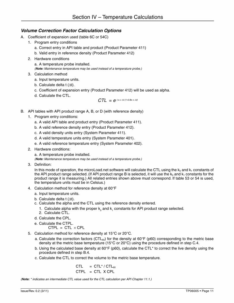
Volume Correction Factor Calculation OptionsA. Coefficient of expansion used (table 6C or 54C) 1. Program entry conditions a. Correct entry in API table and product (Product Parameter 411) b. Valid entry in reference density (Product Parameter 412)

2. Hardware conditions a. A temperature probe installed. (Note: Maintenance temperature may be used instead of a temperature probe.)

3. Calculation method a. Input temperature units. b. Calculate delta t (∆t). c. Coefficient of expansion entry (Product Parameter 412) will be used as alpha. d. Calculate the CTL.

CTL = e (-α × ∆t (1+0.8α × ∆t)

B. API tables with API product range A, B, or D (with reference density) 1. Program entry conditions: a. A valid API table and product entry (Product Parameter 411). b. A valid reference density entry (Product Parameter 412). c. A valid density units entry (System Parameter 411). d. A valid temperature units entry (System Parameter 401). e. A valid reference temperature entry (System Parameter 402).

2. Hardware conditions: a. A temperature probe installed. (Note: Maintenance temperature may be used instead of a temperature probe.)

3. Definition:In this mode of operation, the microLoad.net software will calculate the CTL using the k0 and k1 constants of the API product range selected. (If API product range B is selected, it will use the k0 and k1 constants for the product range it is measuring.) All related entries shown above must correspond. If table 53 or 54 is used, the temperature units must be in Celsius.)

4. Calculation method for reference density at 60°F a. Input temperature units. b. Calculate delta t (∆t). c. Calculate the alpha and the CTL using the reference density entered. 1. Calculate alpha with the proper k0 and k1 constants for API product range selected. 2. Calculate CTL. d. Calculate the CPL. e. Calculate the CTPL. CTPL = CTL × CPL

5. Calculation method for reference density at 15°C or 20°C.a. Calculate the correction factors (CTL60) for the density at 60°F (p60) corresponding to the metric base

density at the metric base temperature (15°C or 20°C) using the procedure defined in step C.4.b. Using the calculated base density at 60°F (p60), calculate the CTL* to correct the live density using the

procedure defined in step B.4.c. Calculate the CTL to correct the volume to the metric base temperature.

CTL = CTL* / CTL60

CTPL = CTL X CPL

(Note: * indicates an intermediate CTL value used for the CTL calculation per API Chapter 11.1.)

• TP06005 Issue/Rev. 0.2 (3/11)


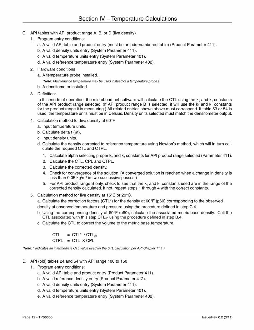
C. API tables with API product range A, B, or D (live density) 1. Program entry conditions: a. A valid API table and product entry (must be an odd-numbered table) (Product Parameter 411). b. A valid density units entry (System Parameter 411). c. A valid temperature units entry (System Parameter 401). d. A valid reference temperature entry (System Parameter 402).

2. Hardware conditions a. A temperature probe installed. (Note: Maintenance temperature may be used instead of a temperature probe.)

b. A densitometer installed.

3. Definition:In this mode of operation, the microLoad.net software will calculate the CTL using the k0 and k1 constants of the API product range selected. (If API product range B is selected, it will use the k0 and k1 constants for the product range it is measuring.) All related entries shown above must correspond. If table 53 or 54 is used, the temperature units must be in Celsius. Density units selected must match the densitometer output.

4. Calculation method for live density at 60°F a. Input temperature units. b. Calculate delta t (∆t). c. Input density units.

d. Calculate the density corrected to reference temperature using Newton’s method, which will in turn cal-culate the required CTL and CTPL.

1. Calculate alpha selecting proper k0 and k1 constants for API product range selected (Parameter 411).2. Calculate the CTL, CPL and CTPL.3. Calculate the corrected density.4. Check for convergence of the solution. (A converged solution is reached when a change in density is

less than 0.05 kg/m3 in two successive passes.)5. For API product range B only, check to see that the k0 and k1 constants used are in the range of the

corrected density calculated. If not, repeat steps 1 through 4 with the correct constants.

5. Calculation method for live density at 15°C or 20°C.a. Calculate the correction factors (CTL*) for the density at 60°F (p60) corresponding to the observeddensity at observed temperature and pressure using the procedure defined in step C.4.b. Using the corresponding density at 60°F (p60), calculate the associated metric base density. Call the

CTL associated with this step CTL60 using the procedure defined in step B.4.c. Calculate the CTL to correct the volume to the metric base temperature.

CTL = CTL* / CTL60

CTPL = CTL X CPL

(Note: * indicates an intermediate CTL value used for the CTL calculation per API Chapter 11.1.)

D. API (old) tables 24 and 54 with API range 100 to 150 1. Program entry conditions: a. A valid API table and product entry (Product Parameter 411). b. A valid reference density entry (Product Parameter 412). c. A valid density units entry (System Parameter 411). d. A valid temperature units entry (System Parameter 401). e. A valid reference temperature entry (System Parameter 402).

Issue/Rev. 0.2 (3/11) TP06005 • Page 13

2. Hardware conditions: a. A temperature probe is installed. (Note: Maintenance temperature may be used instead of the temperature probe.)

3. Definition:In this mode of operation, the microLoad.net software will use the reference density and the current tempera-ture to retrieve the CTL from the selected table. (If table 24 is selected, temperature units must be Fahrenheit. If table 54 is selected, temperature units must be Celsius.)

4. Calculation method a. Input temperature units. b. Using the temperature and reference density, go to the proper table (24 or 54) and select the proper CTL.

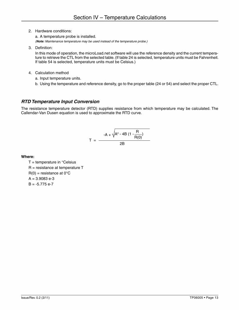
RTD Temperature Input ConversionThe resistance temperature detector (RTD) supplies resistance from which temperature may be calculated. The Callendar-Van Dusen equation is used to approximate the RTD curve.

Where: T = temperature in °Celsius R = resistance at temperature T R(0) = resistance at 0°C A = 3.9083 e-3 B = -5.775 e-7


T = -A + √A2 - 4B (1 -

R )

R(0)

2B

• TP06005 Issue/Rev. 0.2 (3/11)

Section V – Pressure Calculations

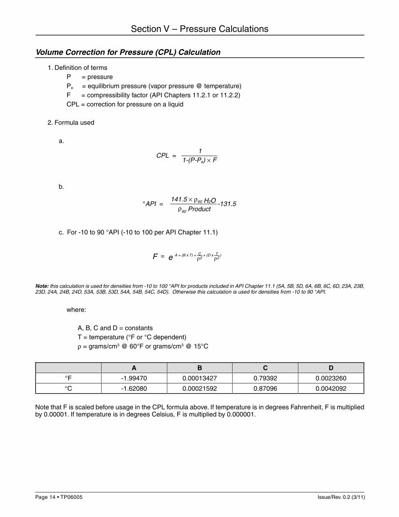
Volume Correction for Pressure (CPL) Calculation

1. Definition of terms P = pressure Pe = equilibrium pressure (vapor pressure @ temperature) F = compressibility factor (API Chapters 11.2.1 or 11.2.2) CPL = correction for pressure on a liquid

2. Formula used

a.

b.

c. For -10 to 90 °API (-10 to 100 per API Chapter 11.1)

Note: this calculation is used for densities from -10 to 100 °API for products included in API Chapter 11.1 (5A, 5B, 5D, 6A, 6B, 6C, 6D, 23A, 23B, 23D, 24A, 24B, 24D, 53A, 53B, 53D, 54A, 54B, 54C, 54D). Otherwise this calculation is used for densities from -10 to 90 °API.

where:

A, B, C and D = constants T = temperature (°F or °C dependent) ρ = grams/cm3 @ 60°F or grams/cm3 @ 15°C

A B C D

°F -1.99470 0.00013427 0.79392 0.0023260

°C -1.62080 0.00021592 0.87096 0.0042092

Note that F is scaled before usage in the CPL formula above. If temperature is in degrees Fahrenheit, F is multiplied by 0.00001. If temperature is in degrees Celsius, F is multiplied by 0.000001.

CPL = 1

1-(P-Pe) × F

°API = 141.5 × ρ60 H2O -131.5

ρ60 Product

F = e A + (B x T) + C + (D x T )ρ2 ρ2

Issue/Rev. 0.2 (3/11) TP06005 • Page 15

Section V – Pressure Calculations

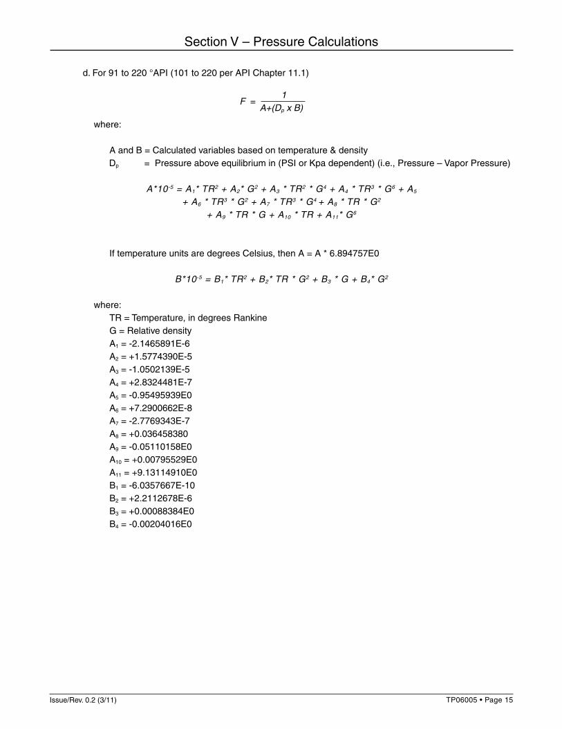
d. For 91 to 220 °API (101 to 220 per API Chapter 11.1)

where: A and B = Calculated variables based on temperature & density Dp = Pressure above equilibrium in (PSI or Kpa dependent) (i.e., Pressure – Vapor Pressure)

A*10-5 = A1* TR2 + A2* G2 + A3 * TR2 * G4 + A4 * TR3 * G6 + A5 + A6 * TR3 * G2 + A7 * TR3 * G4 + A8 * TR * G2

+ A9 * TR * G + A10 * TR + A11* G6

If temperature units are degrees Celsius, then A = A * 6.894757E0

B*10-5 = B1* TR2 + B2* TR * G2 + B3 * G + B4* G2

where: TR = Temperature, in degrees Rankine G = Relative density A1 = -2.1465891E-6 A2 = +1.5774390E-5 A3 = -1.0502139E-5 A4 = +2.8324481E-7 A5 = -0.95495939E0 A6 = +7.2900662E-8 A7 = -2.7769343E-7 A8 = +0.036458380 A9 = -0.05110158E0 A10 = +0.00795529E0 A11 = +9.13114910E0 B1 = -6.0357667E-10 B2 = +2.2112678E-6 B3 = +0.00088384E0 B4 = -0.00204016E0

F = 1

A+(Dp x B)

• TP06005 Issue/Rev. 0.2 (3/11)

Section IV – Pressure Calculations

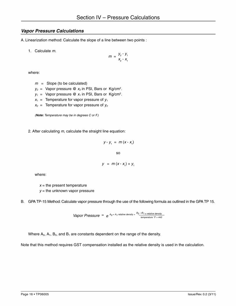
Vapor Pressure Calculations

A. Linearization method: Calculate the slope of a line between two points :

1. Calculate m.m =

y2 - y1

x2 - x1

where:

m = Slope (to be calculated) y2 = Vapor pressure @ x2 in PSI, Bars or Kg/cm2. y1 = Vapor pressure @ x1 in PSI, Bars or Kg/cm2. x1 = Temperature for vapor pressure of y1

x2 = Temperature for vapor pressure of y2

(Note: Temperature may be in degrees C or F.)

2. After calculating m, calculate the straight line equation:

y - y1 = m (x - x1)

so

y = m (x - x1) + y1

where:

x = the present temperature y = the unknown vapor pressure

B. GPA TP-15 Method: Calculate vapor pressure through the use of the following formula as outlined in the GPA TP 15.

Where A0, A1, B0, and B1 are constants dependent on the range of the density.

Note that this method requires GST compensation installed as the relative density is used in the calculation.

Vapor Pressure = e A0 + A1 relative density + B0

+B1 x relative density

temperature °F = 443

Issue/Rev. 0.2 (3/11) TP06005 • Page 17

Section VI – Load Average Calculations

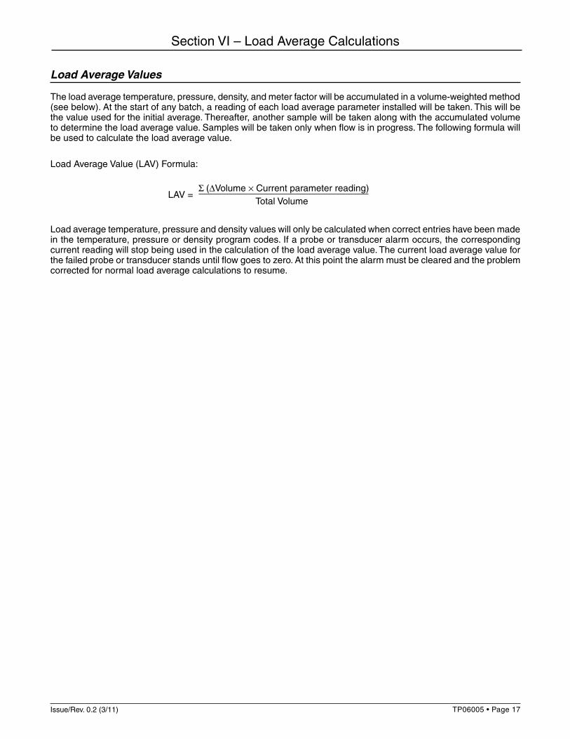
Load Average Values

The load average temperature, pressure, density, and meter factor will be accumulated in a volume-weighted method (see below). At the start of any batch, a reading of each load average parameter installed will be taken. This will be the value used for the initial average. Thereafter, another sample will be taken along with the accumulated volume to determine the load average value. Samples will be taken only when flow is in progress. The following formula will be used to calculate the load average value.

Load Average Value (LAV) Formula:

Load average temperature, pressure and density values will only be calculated when correct entries have been made in the temperature, pressure or density program codes. If a probe or transducer alarm occurs, the corresponding current reading will stop being used in the calculation of the load average value. The current load average value for the failed probe or transducer stands until flow goes to zero. At this point the alarm must be cleared and the problem corrected for normal load average calculations to resume.

LAV = Σ (∆Volume × Current parameter reading)

Total Volume

• TP06005 Issue/Rev. 0.2 (3/11)

Section IV – Diagrams

Auto Prove Meter Factor Calculations

The following equations are used by the microLoad.net to calculate the new meter factor.

CTSP (Correction for Temperature on Steel of a Prover)

where T = temperature of the provery = coefficient of cubical expansion, a constant, 0.0000186 for mild steelt ref = reference temperature (System Parameter 402)

CTLP (Correction for Temperature on Liquid in a Prover)

where e = the exponential constant ∆t = ∆ temperature = actual temperature of the prover - reference temperature (System Parameter 402) α = k0/(ρ60)2 + (k1/ρ60) where k0 and k1 are constants determined based on the product group ρ60 = (141.5 * weight of H2O)/(131.5 + API) OR α = A + (B/(ρ60)2) where A and B are constants for a special range of API gravities ρ60 = (141.5 * weight of H2O)/(131.5 + API)

Combined Correction Factor (CCF) For a Prover

CCFP = CTSP * CTLP

where CTSP and CTLP are as shown above

Corrected Prover Volume

Corrected Prover Volume = Base Prover Volume * CCFP

where Base Prover Volume is as determined by a waterdraw CCFP is as shown above

CTLP = e ( α • ∆t (1 + 0.8α • ∆t))

CTSP = 1 + ((T-tref) * y)

Issue/Rev. 0.2 (3/11) TP06005 • Page 19

Section IV – Diagrams

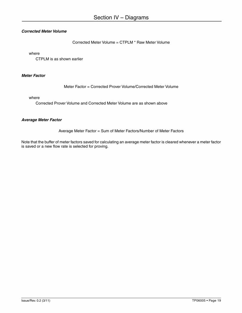
Corrected Meter Volume

Corrected Meter Volume = CTPLM * Raw Meter Volume

where CTPLM is as shown earlier

Meter Factor

Meter Factor = Corrected Prover Volume/Corrected Meter Volume

where Corrected Prover Volume and Corrected Meter Volume are as shown above

Average Meter Factor

Average Meter Factor = Sum of Meter Factors/Number of Meter Factors

Note that the buffer of meter factors saved for calculating an average meter factor is cleared whenever a meter factor is saved or a new flow rate is selected for proving.

Printed in U.S.A. © 3/11 FMC Technologies Measurement Solutions, Inc. All rights reserved. TP06005 Issue/Rev. 0.2 (3/11)

Visit our website at www.fmctechnologies.com/measurementsolutions

The specifications contained herein are subject to change without notice and any user of said specifications should verify from the manufacturer that the specifications are currently in effect. Otherwise, the manufacturer assumes no responsibility for the use of specifications which may have been changed and are no longer in effect.

Contact information is subject to change. For the most current contact information, visit our website at www.fmctechnologies.com/measurementsolutions and click on the “Contact Us” link in the left-hand column.

Headquarters:500 North Sam Houston Parkway West, Suite 100, Houston, TX 77067 USA, Phone: +1 (281) 260 2190, Fax: +1 (281) 260 2191

Measurement Products and Equipment: Erie, PA USA +1 (814) 898 5000Ellerbek, Germany +49 (4101) 3040Barcelona, Spain +34 (93) 201 0989Beijing, China +86 (10) 6500 2251Buenos Aires, Argentina +54 (11) 4312 4736Burnham, England +44 (1628) 603205

Dubai, United Arab Emirates +971 (4) 883 0303Los Angeles, CA USA +1 (310) 328 1236Melbourne, Australia +61 (3) 9807 2818Moscow, Russia +7 (495) 5648705Singapore, +65 6861 3011Thetford, England +44 (1842) 822900

Integrated Measurement Systems:Corpus Christi, TX USA +1 (361) 289 3400Kongsberg, Norway +47 (32) 286700Dubai, United Arab Emirates +971 (4) 883 0303

Revision included in TP06005 Issue/Rev. 0.2 (3/11): Page 10: Addition of Tables 23E, 24E, 53E, 54E, 59E and 60E to Temperature Calculations

smith meter microloadinfo.smithmeter.com/literature/docs/tp06005.pdfvolume correction for...

Documents