slides for chapter 2: examples of economic equilibrium...
TRANSCRIPT

1
Slides for Chapter 2: Examples of economic equilibrium problemstranslated into GAMS
Copyright: James R. Markusen University of Colorado, Boulder
Tools of Economic Analysis - introducing the “third way”
(1) Traditional analytical theory models (“pencil and paper”technology)
(2) Econometric estimation and testing.
(3) Computer simulation modeling - the focus of this course
(A) for use in economic theory: allows us to construct andanalyze theories that are much more complex thanthose tractable in traditional analytical models

“Many branches of both pure and appliedmathematics are in great need of computinginstruments to break the present stalemate createdby the failure of the purely analytical approach tononlinear problems”
--- John Von Neumann, 1945

2
(B) for use in calculating counter-factual outcomes (e.g.,due to policy changes) in empirical models
(C) in both cases, for calculating numerical values forwelfare changes and optimal values for policyvariables.
(4) Two ways of formulating economic models
(A) as an constrained optimization problem
(B) as a complementarity problem: square system ofequations/inequalities and unknowns

3
2.1 Simple supply-demand problem illustrating complementarity
Supply and demand model of a single market, a partial equilibriummodel. Two equations, supply and demand, two variables, priceand quantity.
Economic equilibrium problems are thus represented as a system ofn equations/inequalities in n unknowns.
Complementarity involves (a) associating each equation with a particular variable, called the
complementary variable.
(b) if the variables are restricted to be non-negative (prices andquantities), then the equations are written as weakinequalities.

4
If the equation holds as an equality in equilibrium, then thecomplementary variable is generally strictly positive.
If the equation holds as a strict inequality in equilibrium, thecomplementary variable is zero.
Supply of good X with price P. The supply curve exploits the firm’soptimization decision, equating price with marginal cost: P = MC.
MC $ P with the complementarity condition that X $ 0
Note that the price equation is complementary with a quantityvariable.

5
Suppose that COST = aX + (b/2)X2.
Marginal cost is then given by MC = a + bX.
a + bX $ P complementary with X $ 0.
Optimizing consumer utility for a given income and prices will yield ademand function of the form X = D(P, M) where M is income.
X $ D(P, M) with the complementary condition that P $ 0.
Note that the quantity equation is complementary with a pricevariable.

6
We will suppress income and assume a simple function:
X = c + dP where c > 0, d < 0.
X $ c + dP complementary with P $ 0.
How do we know which inequality is associate with which variableand the direction of the inequality?
Economic theory tells you which variable must be associated withwhich inequality and which way the inequality goes.
(1) ask the question whether or not a particular direction of theinequality is consistent with economic equilibrium.

7
(2) ask the question, “what must be true if the inequality is strict inequilibrium”?
MC < P cannot be an equilibrium, there is a profit opportunity andmore of the good will be produced.
MC > P can be an equilibrium: the good is unprofitable and is notproduced. Thus X is complementary with the supply equation.
X < D(P,M) cannot be an equilibrium, excess demand will cause theprice to rise and more will be supplied.
X > D(P,M) can be an equilibrium, this must mean that the good isfree, and P = 0. Thus P is complementary with the demandequation.

8
2. Coding an economic equilibrium problem in GAMS
First, comment statements can be used at the beginning of thecode, preceded with a *, in the first column of a line. Actual code isshown in courier font.
$TITLE: M2-1.GMS introductory model using MCP* simple supply and demand model (partial equilibrium)
Now we can begin a series of declaration and assignmentstatements.
PARAMETERS A intercept of supply on the P axis (MC at Q = 0) B slope of supply: this is dP over dQ C demand on the Q axis (demand at P = 0) D (inverse) slope of demand, dQ over dP TAX a tax rate used later for experiments;

9
Parameters must be assigned values before the model is solved These parameter values are referred to as Case 1 below. A = 2;C = 6;B = 1;D = -1;TAX = 0;
Now we declare a list of variables. They must be restricted to bepositive to make any economic sense, so declaring them as “positivevariables” tells GAMS to set lower bounds of zero on these variables.
NONNEGATIVE VARIABLES P price of good X X quantity of good X;
Now we similarly declare a list of equations. We can name them

10
anything we want provided it is a name not otherwise in use or, ofcourse, a keyword.
EQUATIONS DEMAND supply relationship (mc cost ge price) SUPPLY quantity demanded as a function of price;
Specify equations. Format: equation name followed by two periods(full stops).
Then after a space, the equation is written out, with =G= GAMScode for “greater than or equal to”.
SUPPLY.. A + B*X =G= P; DEMAND.. X =G= C + D*P;

11
Next we need to declare a model: a set of equations and unknowns.The format is the keyword model, followed by a model name ofyour choosing. Here we use equil.
Next comes a “/” followed by a list of the equation names: eachequation ends with a period followed by the name of thecomplementary variable.
MODEL EQUIL /SUPPLY.X, DEMAND.P/;
Finally, we need to tell GAMS to solve the model and what softwareis needed (GAMS does many other types of problems, such asoptimization)
SOLVE EQUIL USING MCP;
12
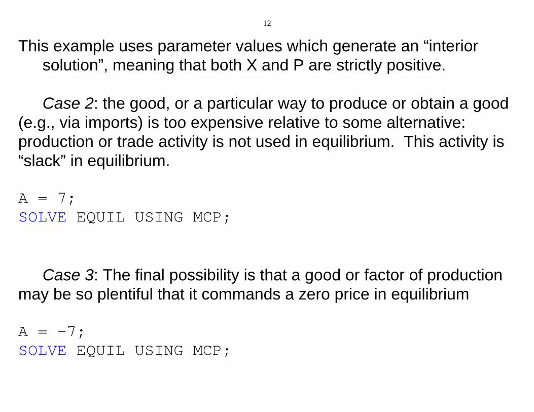
This example uses parameter values which generate an “interiorsolution”, meaning that both X and P are strictly positive.
Case 2: the good, or a particular way to produce or obtain a good(e.g., via imports) is too expensive relative to some alternative:production or trade activity is not used in equilibrium. This activity is“slack” in equilibrium.
A = 7;SOLVE EQUIL USING MCP;
Case 3: The final possibility is that a good or factor of productionmay be so plentiful that it commands a zero price in equilibrium
A = -7;SOLVE EQUIL USING MCP;

Case 1: interior solution
Supply (MC):slope = B
Demand: slope = 1/D
A C
Figure 1: Three outcomes of partial equilibrium example
Case 2: X is too expensive, not produce in equilibrium (X = 0)
Supply (MC)
Demand
A
Case 3: excess supply, X is a free good in equilibrium (P = 0)
Supply (MC)Demand
A
P
X
P
X
P
X

13
3. Counterfactual (comparative statics) experiments
In the following example, we use a parameter called “TAX”, an advalorem tax on the input (marginal cost) to production.
To do so, we declare and specify an additional equation “SUPPLY2"and model “EQUIL2" (GAMS does not allow us to simply rewritethe equation or use the old model name once we name a newequation).
Three parameters are declared and used to extract information afterwe solve the model.
PARAMETERS CONSPRICE consumer price PRODPRICE producer price (equal to marginal cost) TAXREV tax revenue (tax base is producer price);
14
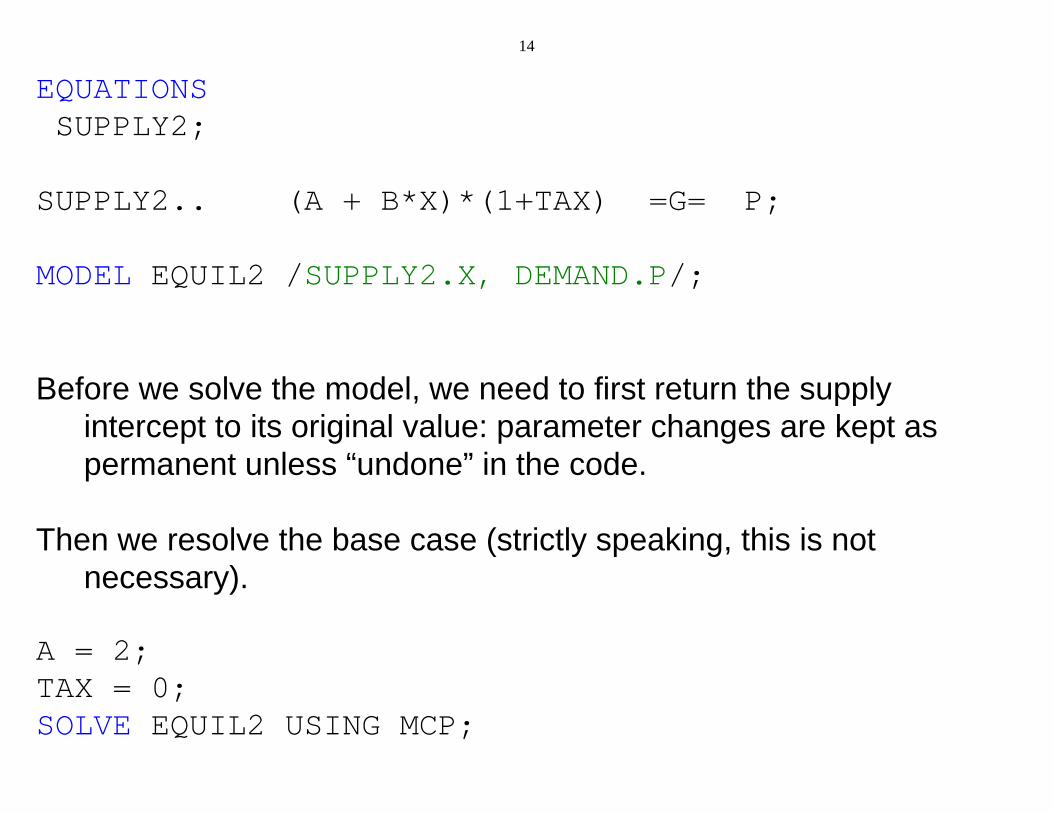
EQUATIONS SUPPLY2;
SUPPLY2.. (A + B*X)*(1+TAX) =G= P;
MODEL EQUIL2 /SUPPLY2.X, DEMAND.P/;
Before we solve the model, we need to first return the supplyintercept to its original value: parameter changes are kept aspermanent unless “undone” in the code.
Then we resolve the base case (strictly speaking, this is notnecessary).
A = 2;TAX = 0;SOLVE EQUIL2 USING MCP;

15
Now set the tax at 25% and solve the model.
TAX = 0.25;SOLVE EQUIL2 USING MCP;
After we solve the model, it is common to extract output using GAMScode.
Note that with the tax specified on inputs, the price being solved for isthe consumer price (price paid by the consumer) not the producerprice (price received by the producer).
Producer price is the same as marginal cost.
GAMS stores three values for variables: its current value, its upperbound (infinity in our case) and its lower bound (zero in our case).

16
When the modeler wants the value of a variable, you have to use thenotation NAME.L where the L stands for level.
GAMS does not automatically print out the values of parameters inthe solution, so you have to ask GAMS to DISPLAY these values.
CONSPRICE = P.L;PRODPRICE = P.L/(1+TAX);TAXREV = PRODPRICE*TAX*X.L;
DISPLAY CONSPRICE, PRODPRICE, TAXREV;

17
4. Reading the output
Again, you need to consult the GAMS users’ manual to see how torun the model, and to read and interpret output once you run themodel.
There is a lot of “stuff” in GAMS listing (output) files, which arestored as FILENAME.LST after you run the model (LST is for“listing file”). Here are just the relevant parts of our model runs
S O L V E S U M M A R Y
MODEL EQUIL TYPE MCP SOLVER MILES FROM LINE 50
**** SOLVER STATUS 1 NORMAL COMPLETION **** MODEL STATUS 1 OPTIMAL

18
Case 1: The LEVEL is the solution value of the variables. MARGINAL indicates the degree to which the equationcorresponding to the variable is out of equality.
For P (price), the equation is DEMAND and the value of themarginal is supply minus demand. For X (quantity), theequation is SUPPLY and the value of the marginal is the excessof marginal cost over price.
Variables that have positive values in the solution should have zeromarginals.
Variables that have zero values in the solution should have positivemarginals.
LOWER LEVEL UPPER MARGINAL
---- VAR P . 4.000 +INF ---- VAR X . 2.000 +INF
19
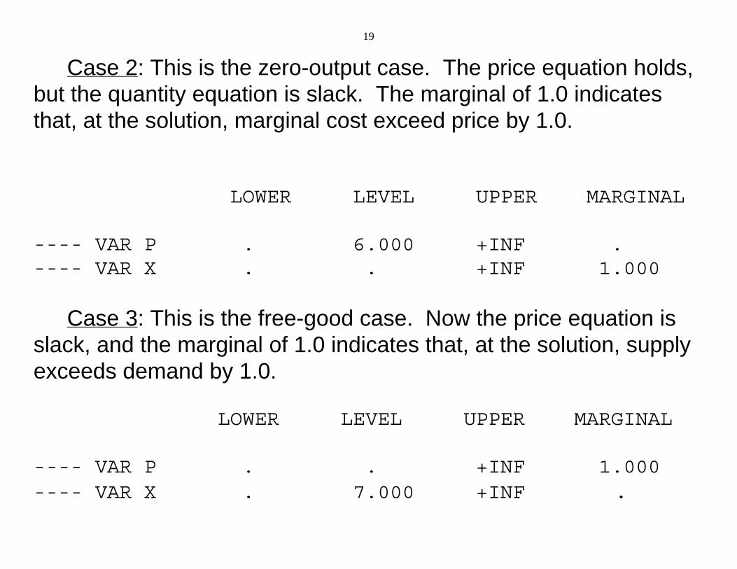
Case 2: This is the zero-output case. The price equation holds,but the quantity equation is slack. The marginal of 1.0 indicatesthat, at the solution, marginal cost exceed price by 1.0.
LOWER LEVEL UPPER MARGINAL
---- VAR P . 6.000 +INF . ---- VAR X . . +INF 1.000
Case 3: This is the free-good case. Now the price equation isslack, and the marginal of 1.0 indicates that, at the solution, supplyexceeds demand by 1.0. LOWER LEVEL UPPER MARGINAL
---- VAR P . . +INF 1.000 ---- VAR X . 7.000 +INF .
20
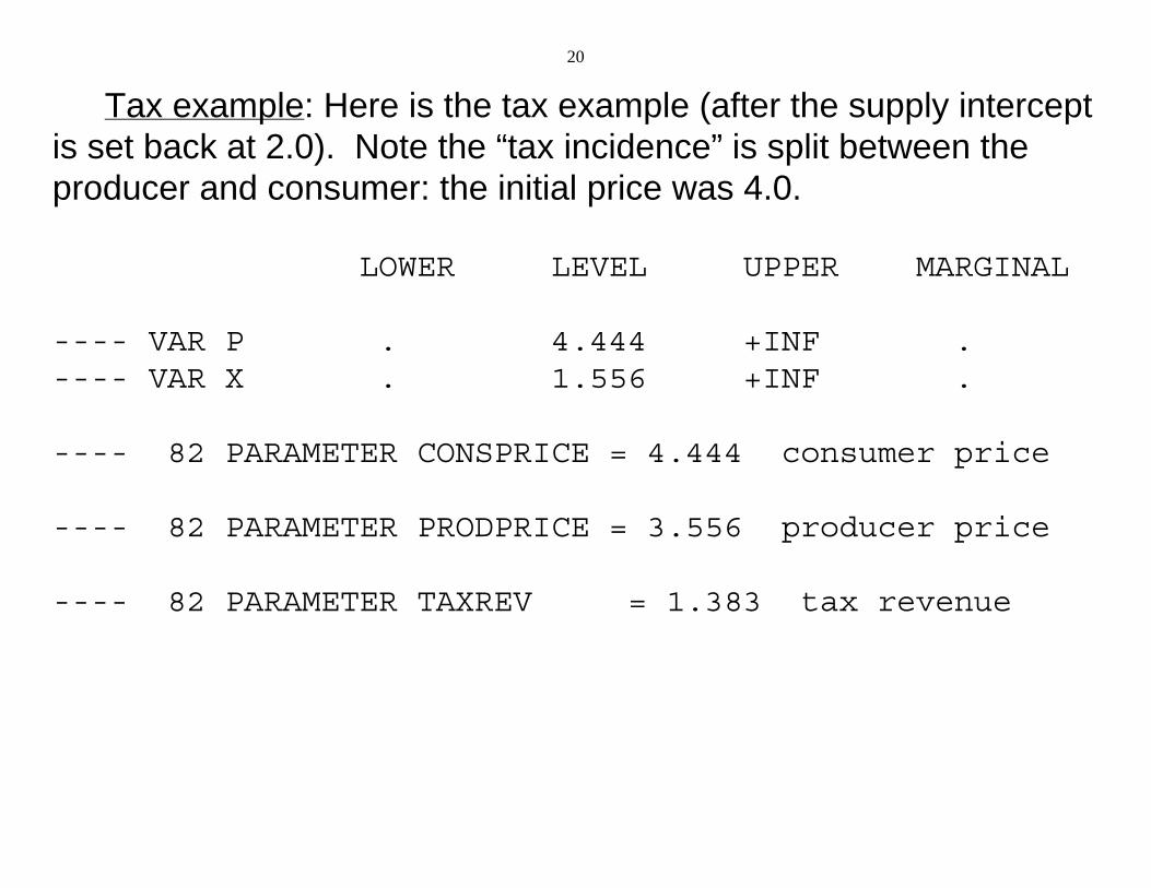
Tax example: Here is the tax example (after the supply interceptis set back at 2.0). Note the “tax incidence” is split between theproducer and consumer: the initial price was 4.0.
LOWER LEVEL UPPER MARGINAL
---- VAR P . 4.444 +INF . ---- VAR X . 1.556 +INF . ---- 82 PARAMETER CONSPRICE = 4.444 consumer price
---- 82 PARAMETER PRODPRICE = 3.556 producer price
---- 82 PARAMETER TAXREV = 1.383 tax revenue

C:\jim\COURSES\8858\code-bk 2012\M2-1.gms Monday, January 09, 2012 3:08:17 AM Page 1
$TITLE: M2-1.GMS introductory model using MCP* simple supply and demand model (partial equilibrium)
PARAMETERS A intercept of supply on the P axis (MC at Q = 0) B change in MC in response to Q - this is dP over dQ C intercept of demand on the Q axis (demand at P = 0) D response of demand to changes in price - dQ over dP T A X a tax rate used later for experiments;
A = 2;C = 6;B = 1;D = -1;
NONNEGATIVE VARIABLES P price of good X X quantity of good X;
EQUATIONS S U P P L Y supply relationship (marginal cost ge price) D E M A N D quantity demanded as a function of price;
SUPPLY.. A + B*X =G= P;
C:\jim\COURSES\8858\code-bk 2012\M2-1.gms Monday, January 09, 2012 3:08:17 AM Page 2
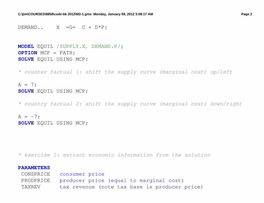
DEMAND.. X =G= C + D*P;
MODEL EQUIL /SUPPLY.X, DEMAND.P/;OPTION MCP = PATH;SOLVE EQUIL USING MCP;
* counter factual 1: shift the supply curve (marginal cost) up/left
A = 7;SOLVE EQUIL USING MCP;
* country factual 2: shift the supply curve (marginal cost) down/right
A = -7;SOLVE EQUIL USING MCP;
* exercise 1: extract economic information from the solution
PARAMETERS C O N S P R I C E consumer price P R O D P R I C E producer price (equal to marginal cost) T A X R E V tax revenue (note tax base is producer price)
C:\jim\COURSES\8858\code-bk 2012\M2-1.gms Monday, January 09, 2012 3:08:17 AM Page 3
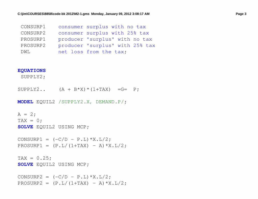
C O N S U R P 1 consumer surplus with no tax C O N S U R P 2 consumer surplus with 25% tax P R O S U R P 1 producer "surplus" with no tax P R O S U R P 2 producer "surplus" with 25% tax D W L net loss from the tax;
EQUATIONS SUPPLY2;
SUPPLY2.. (A + B*X)*(1+TAX) =G= P;
MODEL EQUIL2 /SUPPLY2.X, DEMAND.P/;
A = 2;TAX = 0;SOLVE EQUIL2 USING MCP;
CONSURP1 = (-C/D - P.L)*X.L/2;PROSURP1 = (P.L/(1+TAX) - A)*X.L/2;
TAX = 0.25;SOLVE EQUIL2 USING MCP;
CONSURP2 = (-C/D - P.L)*X.L/2;PROSURP2 = (P.L/(1+TAX) - A)*X.L/2;

C:\jim\COURSES\8858\code-bk 2012\M2-1.gms Monday, January 09, 2012 3:08:17 AM Page 4
CONSPRICE = P.L;PRODPRICE = P.L/(1+TAX);TAXREV = PRODPRICE*TAX*X.L;DISPLAY CONSPRICE, PRODPRICE, TAXREV;
DWL = CONSURP1 + PROSURP1 - (CONSURP2 + PROSURP2 + TAXREV);DISPLAY CONSURP1, PROSURP1, CONSURP2, PROSURP2, TAXREV, DWL;
*exercise 2, mismatch the complementary variables
TAX = 0;
MODEL EQUIL3 /SUPPLY.P, DEMAND.X/;
SOLVE EQUIL3 USING MCP;
P.L = 0;X.L = 6;
A = 7;SOLVE EQUIL3 USING MCP;
A = -7;SOLVE EQUIL3 USING MCP;

21
2.2 Maximization of utility subject to a linear budget constraint
Illustrates the use of the GAMS NLP and MCP solvers
NLP non-linear programming
MCP mixed complementarity problem
Cobb-Douglas utility function with linear budget constraint
Result: C-D exponents are expenditure shares:

22
“Primal” formulation as an optimization problem
Can solve for “Marshallian” or “uncompensated” demand functions

23
“Dual” formulation as a minimization problem
Can solve for “Hicksian” or “compensated” demand functions
C:\jim\COURSES\8858\code-bk 2012\M2-2.gms Monday, January 09, 2012 3:34:24 AM Page 1
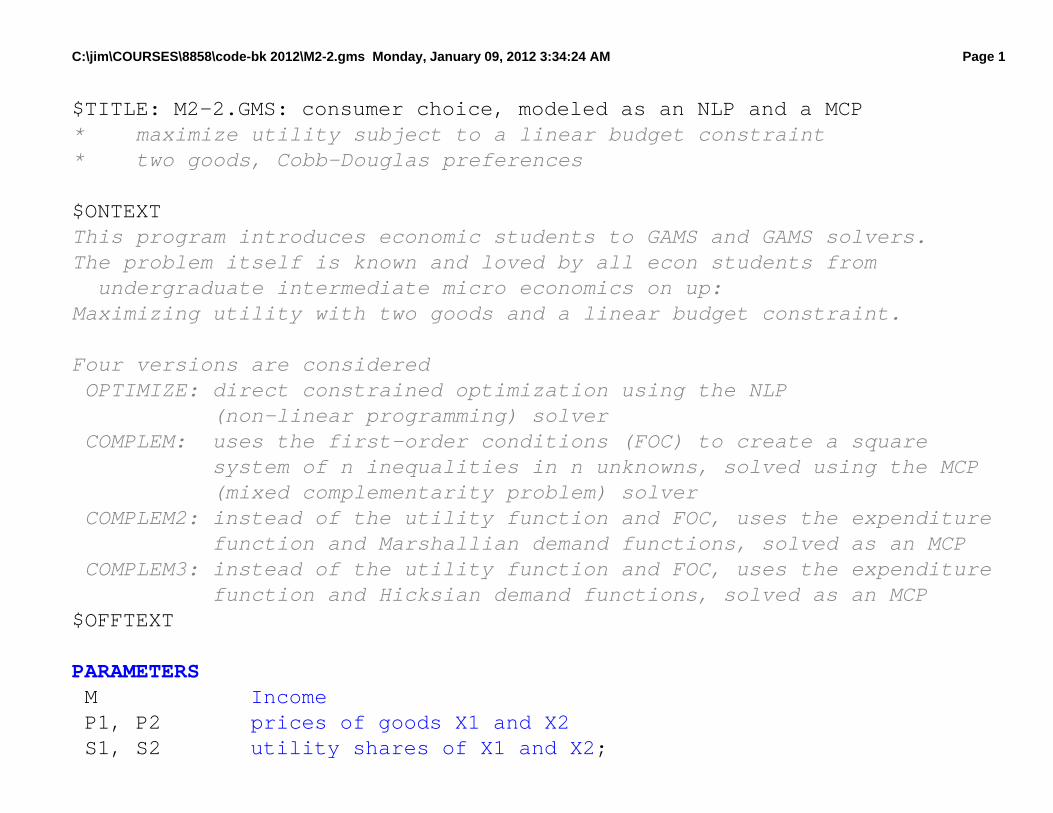
$TITLE: M2-2.GMS: consumer choice, modeled as an NLP and a MCP* maximize utility subject to a linear budget constraint* two goods, Cobb-Douglas preferences
$ONTEXTThis program introduces economic students to GAMS and GAMS solvers.The problem itself is known and loved by all econ students from undergraduate intermediate micro economics on up:Maximizing utility with two goods and a linear budget constraint.
Four versions are considered OPTIMIZE: direct constrained optimization using the NLP (non-linear programming) solver COMPLEM: uses the first-order conditions (FOC) to create a square system of n inequalities in n unknowns, solved using the MCP (mixed complementarity problem) solver COMPLEM2: instead of the utility function and FOC, uses the expenditure function and Marshallian demand functions, solved as an MCP COMPLEM3: instead of the utility function and FOC, uses the expenditure function and Hicksian demand functions, solved as an MCP$OFFTEXT
PARAMETERS M Income P1, P 2 prices of goods X1 and X2 S1, S 2 utility shares of X1 and X2;

C:\jim\COURSES\8858\code-bk 2012\M2-2.gms Monday, January 09, 2012 3:34:24 AM Page 2
M = 100;P1 = 1;P2 = 1;S1 = 0.5;S2 = 0.5;
NONNEGATIVE VARIABLES
X1, X 2 Commodity demands L A M B D A Lagrangean multiplier (marginal utility of income);
VARIABLES
U Welfare;
EQUATIONS
U T I L I T Y Utility I N C O M E Income-expenditure constraint FOC1, F O C 2 First-order conditions for X1 and X2;
UTILITY.. U =E= 2*(X1**S1)*(X2**S2);
INCOME.. M =G= P1*X1 + P2*X2;
C:\jim\COURSES\8858\code-bk 2012\M2-2.gms Monday, January 09, 2012 3:34:24 AM Page 3
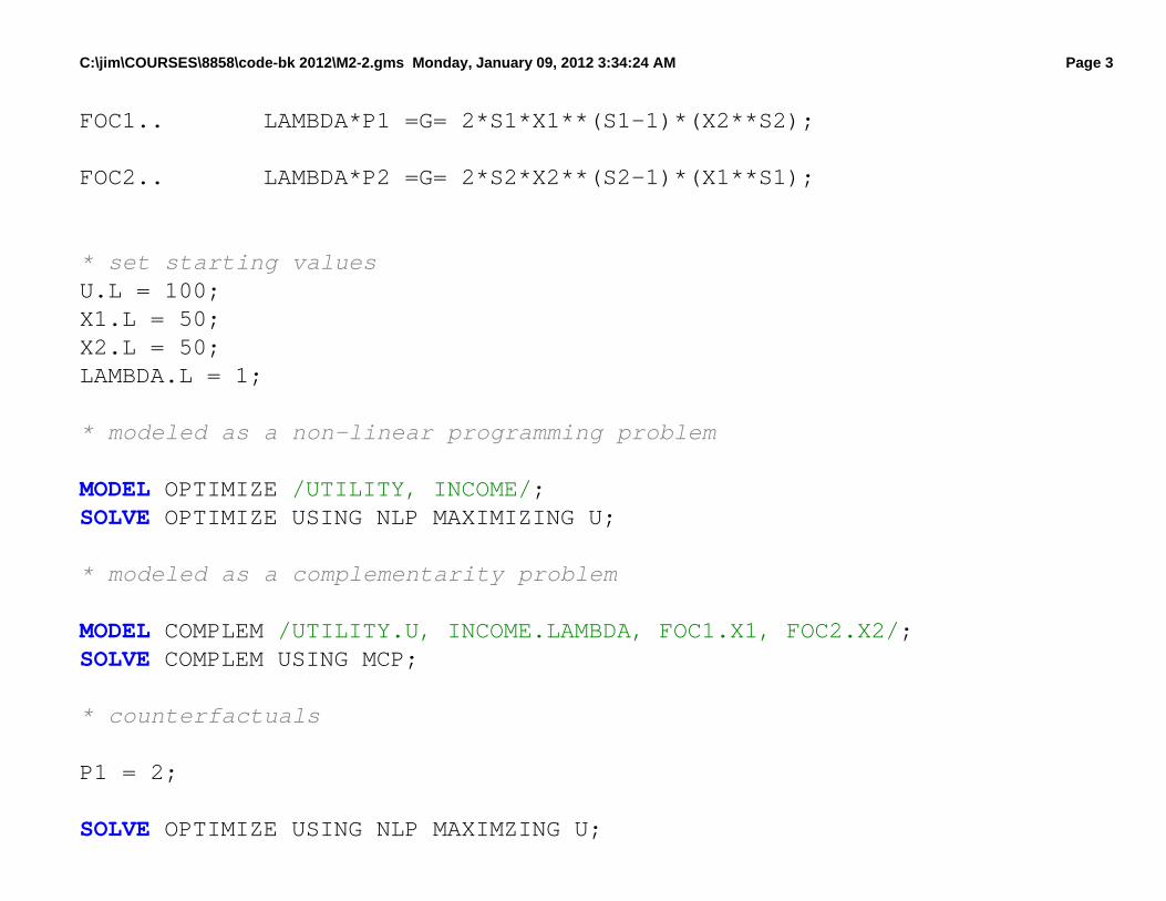
FOC1.. LAMBDA*P1 =G= 2*S1*X1**(S1-1)*(X2**S2);
FOC2.. LAMBDA*P2 =G= 2*S2*X2**(S2-1)*(X1**S1);
* set starting valuesU.L = 100;X1.L = 50;X2.L = 50;LAMBDA.L = 1;
* modeled as a non-linear programming problem
MODEL OPTIMIZE /UTILITY, INCOME/;SOLVE OPTIMIZE USING NLP MAXIMIZING U;
* modeled as a complementarity problem
MODEL COMPLEM /UTILITY.U, INCOME.LAMBDA, FOC1.X1, FOC2.X2/;SOLVE COMPLEM USING MCP;
* counterfactuals
P1 = 2;
SOLVE OPTIMIZE USING NLP MAXIMZING U;

C:\jim\COURSES\8858\code-bk 2012\M2-2.gms Monday, January 09, 2012 3:34:24 AM Page 4
SOLVE COMPLEM USING MCP;
P1 = 1;M = 200;
SOLVE OPTIMIZE USING NLP MAXIMZING U;SOLVE COMPLEM USING MCP;
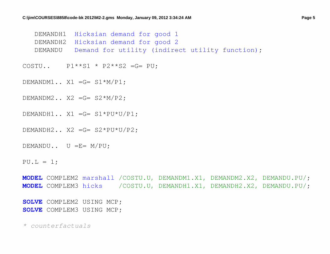
* now use the expenditure function, giving the minimum cost of buying* one unit of utility: COSTU = P1**S1 * P2**S2 = PU* where PU is the "price" of utility: the inverse of lambda* two versions are presented:* one using Marshallian (uncompensated) demand: X_i = F_i(P1, P2, M)* one using Hicksian (compensated) demand: X_i = F_i(P1, P2, U)
P1 = 1;M = 100;
NONNEGATIVE VARIABLES P U price of utility;
EQUATIONS C O S T U expenditure function: cost of producing utility = PU D E M A N D M 1 Marshallian demand for good 1 D E M A N D M 2 Marshallian demand for good 2
C:\jim\COURSES\8858\code-bk 2012\M2-2.gms Monday, January 09, 2012 3:34:24 AM Page 5
D E M A N D H 1 Hicksian demand for good 1 D E M A N D H 2 Hicksian demand for good 2 D E M A N D U Demand for utility (indirect utility function);
COSTU.. P1**S1 * P2**S2 =G= PU;
DEMANDM1.. X1 =G= S1*M/P1;
DEMANDM2.. X2 =G= S2*M/P2;
DEMANDH1.. X1 =G= S1*PU*U/P1;
DEMANDH2.. X2 =G= S2*PU*U/P2;
DEMANDU.. U =E= M/PU;
PU.L = 1;
MODEL C O M P L E M 2 m a r s h a l l /COSTU.U, DEMANDM1.X1, DEMANDM2.X2, DEMANDU.PU/;MODEL C O M P L E M 3 h i c k s /COSTU.U, DEMANDH1.X1, DEMANDH2.X2, DEMANDU.PU/;
SOLVE COMPLEM2 USING MCP;SOLVE COMPLEM3 USING MCP;
* counterfactuals

C:\jim\COURSES\8858\code-bk 2012\M2-2.gms Monday, January 09, 2012 3:34:24 AM Page 6
P1 = 2;
SOLVE COMPLEM2 USING MCP;SOLVE COMPLEM3 USING MCP;
P1 = 1;M = 200;
SOLVE COMPLEM2 USING MCP;SOLVE COMPLEM3 USING MCP;

24
2.3 Extension of utility optimization: add a rationing constraint
Illustrate slackness in equilibrium, illustrate “shadow” pricesRATION $ X1 with Lagrangean multiplier 8r

C:\jim\COURSES\8858\code-bk 2012\M2-3.gms Monday, January 09, 2012 3:45:25 AM Page 1
$TITLE: M2-3.GMS add a rationing constraint to model M2-2* MAXIMIZE UTILITY SUBJECT TO A LINEAR BUDGET CONSTRAINT* PLUS RATIONING CONSTRAINT ON X1* two goods, Cobb-Douglas preferences
PARAMETERS M Income P1, P 2 prices of goods X1 and X2 S1, S 2 util shares of X1 and X2 R A T I O N rationing constraint on the quantity of X1;
M = 100;P1 = 1;P2 = 1;S1 = 0.5;S2 = 0.5;RATION = 100.;
NONNEGATIVE VARIABLES X1, X 2 Commodity demands L A M B D A I Lagrangean multiplier (marginal utility of income) L A M B D A R Lagrangean mulitplier on rationing constraint;
VARIABLES U Welfare;

C:\jim\COURSES\8858\code-bk 2012\M2-3.gms Monday, January 09, 2012 3:45:25 AM Page 2
EQUATIONS U T I L I T Y Utility I N C O M E Income-expenditure constraint R A T I O N 1 Rationing contraint on good X1 FOC1, F O C 2 First-order conditions for X1 and X2;
UTILITY.. U =E= 2*(X1**S1)*(X2**S2);
INCOME.. M =G= P1*X1 + P2*X2;
RATION1.. RATION =G= X1;
FOC1.. LAMBDAI*P1 + LAMBDAR =G= 2*S1*X1**(S1-1)*(X2**S2);
FOC2.. LAMBDAI*P2 =G= 2*S2*X2**(S2-1)*(X1**S1);
* modeled as a non-linear programming problem* set starting values
U.L = 100;X1.L = 50;X2.L = 50;LAMBDAI.L = 1;LAMBDAR.L = 0;
MODEL OPTIMIZE /UTILITY, INCOME, RATION1/;

C:\jim\COURSES\8858\code-bk 2012\M2-3.gms Monday, January 09, 2012 3:45:25 AM Page 3
SOLVE OPTIMIZE USING NLP MAXIMIZING U;
* modeled as a complementarity problem
MODEL COMPLEM /UTILITY.U, INCOME.LAMBDAI, RATION1.LAMBDAR, FOC1.X1, FOC2.X2/;SOLVE COMPLEM USING MCP;
* try binding rationing constraint at X1 <= RATION = 25;
RATION = 25;SOLVE OPTIMIZE USING NLP MAXIMIZING U;SOLVE COMPLEM USING MCP;
* show that shadow price of rationing constraint increases with income* could lead to a black market in rationing coupons, "scalping" tickets
M = 200;SOLVE OPTIMIZE USING NLP MAXIMIZING U;SOLVE COMPLEM USING MCP;
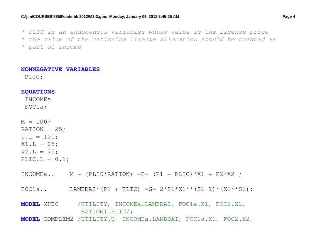
* illustrate the mpec solver* suppose we want to enforce the rationing contraint via licenses for X1* consumers are given an allocation of licenses which is RATION
C:\jim\COURSES\8858\code-bk 2012\M2-3.gms Monday, January 09, 2012 3:45:25 AM Page 4
* PLIC is an endogenous variables whose value is the license price* the value of the rationing license allocation should be treated as* part of income
NONNEGATIVE VARIABLES PLIC;
EQUATIONS INCOMEa FOC1a;
M = 100;RATION = 25;U.L = 100;X1.L = 25;X2.L = 75;PLIC.L = 0.1;
INCOMEa.. M + (PLIC*RATION) =E= (P1 + PLIC)*X1 + P2*X2 ;
FOC1a.. LAMBDAI*(P1 + PLIC) =G= 2*S1*X1**(S1-1)*(X2**S2);
MODEL M P E C /UTILITY, INCOMEa.LAMBDAI, FOC1a.X1, FOC2.X2, RATION1.PLIC/;MODEL COMPLEM2 /UTILITY.U, INCOMEa.LAMBDAI, FOC1a.X1, FOC2.X2,

C:\jim\COURSES\8858\code-bk 2012\M2-3.gms Monday, January 09, 2012 3:45:25 AM Page 5
RATION1.PLIC/;
OPTION MPEC = nlpec;
SOLVE MPEC USING MPEC MAXIMIZING U;SOLVE COMPLEM2 USING MCP;
M = 200;
SOLVE MPEC USING MPEC MAXIMIZING U;SOLVE COMPLEM2 USING MCP;
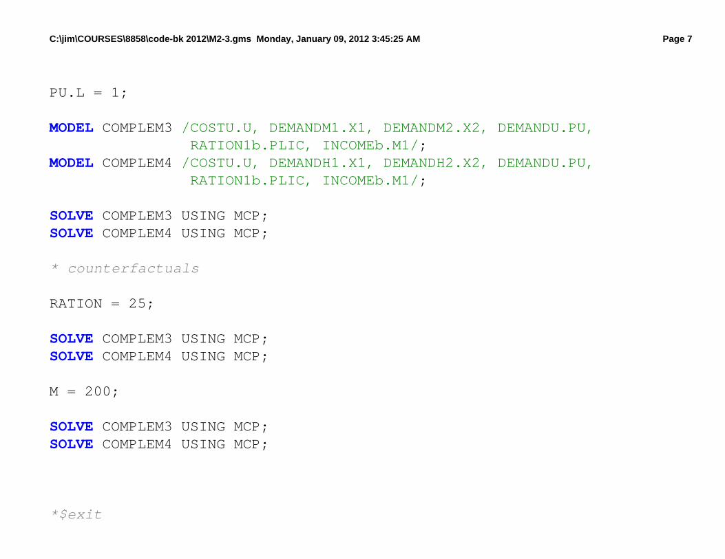
* now use the expenditure function, giving the minimum cost of buying* one unit of utility: COSTU = P1**S1 * P2**S2 = PU* where PU is the "price" of utility: the inverse of lambda* two versions are presented:* one using Marshallian (uncompensated) demand: Xi = F(P1, P2, M)* one using Hicksian (compensated) demand: Xi = F(P1, P2, U)
RATION = 100;M = 100;
NONNEGATIVE VARIABLES P U price of utility M 1 income inclusive of the value of rationing allocation;

C:\jim\COURSES\8858\code-bk 2012\M2-3.gms Monday, January 09, 2012 3:45:25 AM Page 6
EQUATIONS C O S T U expenditure function: cost of producing utility = PU D E M A N D M 1 Marshallian demand for good 1 D E M A N D M 2 Marshallian demand for good 2 D E M A N D H 1 Hicksian demand for good 1 D E M A N D H 2 Hicksian demand for good 2 D E M A N D U Demand for utility (indirect utility function) R A T I O N 1 b Rationing constraint (same as before) I N C O M E b Income balance equation;
COSTU.. (PLIC+P1)**S1 * P2**S2 =G= PU;
DEMANDM1.. X1 =G= S1*M1/(P1+PLIC);
DEMANDM2.. X2 =G= S2*M1/P2;
DEMANDH1.. X1 =G= S1*PU*U/(P1+PLIC);
DEMANDH2.. X2 =G= S2*PU*U/P2;
DEMANDU.. U =E= M1/PU;
RATION1b.. RATION =G= X1;
INCOMEb.. M1 =E= M + PLIC*RATION;
C:\jim\COURSES\8858\code-bk 2012\M2-3.gms Monday, January 09, 2012 3:45:25 AM Page 7
PU.L = 1;
MODEL COMPLEM3 /COSTU.U, DEMANDM1.X1, DEMANDM2.X2, DEMANDU.PU, RATION1b.PLIC, INCOMEb.M1/;MODEL COMPLEM4 /COSTU.U, DEMANDH1.X1, DEMANDH2.X2, DEMANDU.PU, RATION1b.PLIC, INCOMEb.M1/;
SOLVE COMPLEM3 USING MCP;SOLVE COMPLEM4 USING MCP;
* counterfactuals
RATION = 25;
SOLVE COMPLEM3 USING MCP;SOLVE COMPLEM4 USING MCP;
M = 200;
SOLVE COMPLEM3 USING MCP;SOLVE COMPLEM4 USING MCP;
*$exit

C:\jim\COURSES\8858\code-bk 2012\M2-3.gms Monday, January 09, 2012 3:45:25 AM Page 8
* scenario generation
SETS I indexes different values of rationing constraint /I1*I10/ J indexes income levels /J1*J10/;
PARAMETERS RLEVEL(I) PCINCOME(J) LICENSEP(I,J);
U.L = 50;X1.L = 25;X2.L = 25;PLIC.L = 0.;LAMBDAI.L = 1;
* the following is to prevent solver failure when evaluating X1**(S1-1)* at X1 = 0 (given S1-1 < 0)X1.LO = 0.01;X2.LO = 0.01;
LOOP(I,LOOP(J,
RATION = 110 - 10*ORD(I); M = 25 + 25*ORD(J);

C:\jim\COURSES\8858\code-bk 2012\M2-3.gms Monday, January 09, 2012 3:45:25 AM Page 9
SOLVE MPEC USING MPEC MAXIMIZING U;
RLEVEL(I) = RATION; PCINCOME(J) = M; LICENSEP(I,J) = PLIC.L;
););
DISPLAY RLEVEL, PCINCOME, LICENSEP;
$LIBINCLUDE XLDUMP LICENSEP M2-3.XLS SHEET1!B3

C:\jim\COURSES\8858\code-bk 2012\M2-4.gms Monday, January 09, 2012 3:50:09 AM Page 1
$TITLE: M2-4.GMS quick introduction to sets and scenarios using M2-2* MAXIMIZE UTILITY SUBJECT TO A LINEAR BUDGET CONSTRAINT* same as UTIL-OPT1.GMS but introduces set notation
SET I Prices and Goods / X1, X2 /;ALIAS (I, II);
PARAMETER M Income R A T I O N ration of X1 (constraint on max consumption of X1) P(I) prices S(I) util shares;
M = 100;P("X1") = 1;P("X2") = 1;S("X1") = 0.5;S("X2") = 0.5;RATION = 100;
NONNEGATIVE VARIABLES
X(I) Commodity demands L A M B D A I Marginal utility of income (Lagrangean multiplier) L A M B D A R Marginal effect of ration constraint;

C:\jim\COURSES\8858\code-bk 2012\M2-4.gms Monday, January 09, 2012 3:50:09 AM Page 2
VARIABLES
U Welfare;
EQUATIONS
UTILITY INCOME RATION1 FOC(I);
UTILITY.. U =E= 2*PROD(I, X(I)**S(I));
INCOME.. M =G= SUM(I, P(I)*X(I));
RATION1.. RATION =G= X("X1");
FOC(I).. LAMBDAI*P(I) + LAMBDAR$(ORD(I) EQ 1) =G= S(I)*X(I)**(-1)*2*PROD(II, X(II)**S(II));
U.L = 100;X.L(I) = 50;RATION = 100;
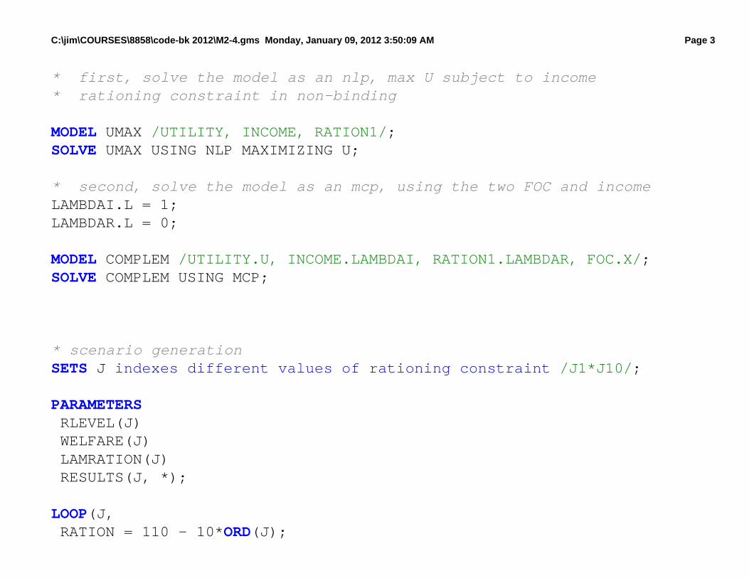
C:\jim\COURSES\8858\code-bk 2012\M2-4.gms Monday, January 09, 2012 3:50:09 AM Page 3
* first, solve the model as an nlp, max U subject to income* rationing constraint in non-binding
MODEL UMAX /UTILITY, INCOME, RATION1/;SOLVE UMAX USING NLP MAXIMIZING U;
* second, solve the model as an mcp, using the two FOC and incomeLAMBDAI.L = 1;LAMBDAR.L = 0;
MODEL COMPLEM /UTILITY.U, INCOME.LAMBDAI, RATION1.LAMBDAR, FOC.X/;SOLVE COMPLEM USING MCP;
* scenario generationSETS J indexes different values of rationing constraint /J1*J10/;
PARAMETERS RLEVEL(J) WELFARE(J) LAMRATION(J) RESULTS(J, *);
LOOP(J, RATION = 110 - 10*ORD(J);

C:\jim\COURSES\8858\code-bk 2012\M2-4.gms Monday, January 09, 2012 3:50:09 AM Page 4
SOLVE COMPLEM USING MCP;
RLEVEL(J) = RATION; WELFARE(J) = U.L; LAMRATION(J) = LAMBDAR.L;
);
RESULTS(J, "RLEVEL") = RLEVEL(J);RESULTS(J, "WELFARE") = WELFARE(J);RESULTS(J, "LAMRATION") = LAMRATION(J);
DISPLAY RLEVEL, WELFARE, LAMRATION, RESULTS;
$LIBINCLUDE XLDUMP RESULTS M2-3.XLS SHEET2!B3

25
2.5 Toward General Equilibrium
We used a partial-equilibrium model to introduce complementarityand the GAMS solver. Now we want to take a step towardgeneral equilibrium.
One household and one firm. The household has a fixed stock oflabor (L).
Further assumption: the household derives no utility from leisure, andso will always supply all labor to the market if the wage rate (W) ispositive.
There is a single good (X) produced from the single input labor.
The firm buys labor services and sells X to the household at price P.

26
The household receives income from selling labor services and usesit all to buy X.
Our model is shown schematically in Figure 2. As noted in theFigure, general equilibrium requires five conditions:
(1) consumer optimization(2) producer optimization(3) supply $ demand for labor(4) supply $ demand for X(5) consumer income equals expenditure (income-expenditure
balance)
The consumer has no alternative use for labor and so optimizes bysupplying it all.
The consumer prefers more X and so the demand for X is going to begiven by X = WL/P: it is optimal to spend all income on X.

Figure 2: General equilibrium
Conditions for general equilibrium
(1) Firms optimize
(2) Consumers optimize
(3) Supply equals demand for labor
(4) Supply equals demand for good X
(5) Income equals expenditure (all labor income is spent on X)
Households Firms
Labor supply
Goods supply
Labor income
Expenditure on goods

25
2.5 Toward General Equilibrium
We used a partial-equilibrium model to introduce complementarityand the GAMS solver. Now we want to take a step towardgeneral equilibrium.
One household and one firm. The household has a fixed stock oflabor (L).
Further assumption: the household derives no utility from leisure, andso will always supply all labor to the market if the wage rate (W) ispositive.
There is a single good (X) produced from the single input labor.
The firm buys labor services and sells X to the household at price P.

26
The household receives income from selling labor services and usesit all to buy X.
Our model is shown schematically in Figure 2. As noted in theFigure, general equilibrium requires five conditions:
(1) consumer optimization(2) producer optimization(3) supply $ demand for labor(4) supply $ demand for X(5) consumer income equals expenditure (income-expenditure
balance)
The consumer has no alternative use for labor and so optimizes bysupplying it all.
The consumer prefers more X and so the demand for X is going to begiven by X = WL/P: it is optimal to spend all income on X.

27
The production function for X will be given as X = "L, where " is themarginal product of labor in X production.
We assume competition and free entry, so that the firm is force toprice at marginal cost.
Marginal cost, the cost of producing one more unit of X, is given byW/" (1/" is the amount of labor needed for one unit of X).
There are two parameters, total labor supply (LBAR) and productivity" (ALPHA).
PARAMETERS LBAR labor supply (fixed and inelastic) ALPHA productivity parameter X = ALPHA*L;
LBAR = 100;
28
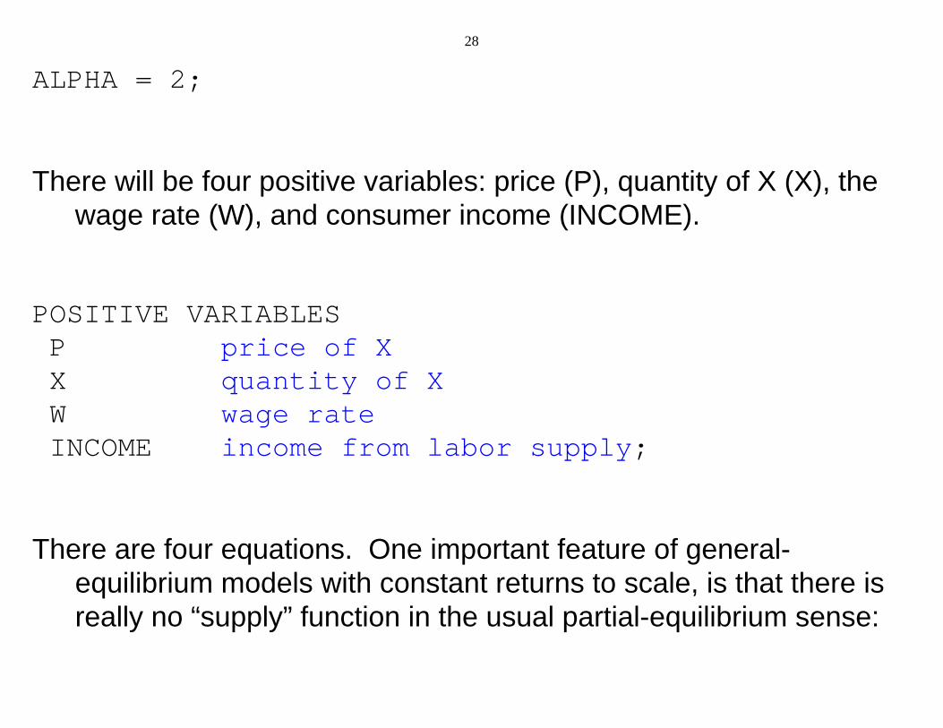
ALPHA = 2;
There will be four positive variables: price (P), quantity of X (X), thewage rate (W), and consumer income (INCOME).
POSITIVE VARIABLES P price of X X quantity of X W wage rate INCOME income from labor supply;
There are four equations. One important feature of general-equilibrium models with constant returns to scale, is that there isreally no “supply” function in the usual partial-equilibrium sense:

29
At given factor prices, the “supply” curve (the marginal cost curve) ishorizontal.
Supply is perfectly elastic at a fixed price P = MC, the latter being aconstant at constant factor prices.
With constant returns, marginal cost is also average cost, and so thisequation can also be thought of as a free-entry, zero-profitscondition.
Accordingly, we refer to this equation as ZPROFIT (zero profits).
Then we require two market-clearing conditions.

30
First, supply of X must be greater than or equal to demand with thecomplementary variable being P, the price of X. This is referredto as CMKTCLEAR (commodity-market clearing).
Second, the supply of labor must be greater than or equal to itsdemand, with the complementary variable being W, the wage rate(price of labor). This is labeled LMKTCLEAR (labor-marketclearing).
Finally, we require income balance: consumer expenditure equalslabor income. This is labeled CONSINCOME.
EQUATIONS ZPROFIT zeroprofits in X production CMKTCLEAR commodity (X) market clearing LMKTCLEAR labor market clearing CONSINCOME consumer income;

31
Marginal cost is just the wage rate divided by ".
Commodity market clearing: X is greater than or equal to demand,which is just income divided by P, the price of X.
Labor-market clearing: supply, LBAR, is greater than or equal tolabor demand, given by X divided by " (X/").
Income spent on X must equal wage income, W times LBAR(W*LBAR).
ZPROFIT.. W/ALPHA =G= P;
CMKTCLEAR.. X =G= INCOME/P;
LMKTCLEAR.. LBAR =G= X/ALPHA;
CONSINCOME.. INCOME =G= W*LBAR;

32
We name the model “GE” for general equilibrium, and associate eachequation in the model with its complementary variable.
MODEL GE /ZPROFIT.X, CMKTCLEAR.P, LMKTCLEAR.W, CONSINCOME.INCOME/;
Setting starting values of variables. Helps the solver find thesolution, important in complex problems. The notation for setting aninitial value of a variable is the NAME.L notation we used earlier.
* set some starting values
P.L = 1;W.L = 1;X.L = 200;INCOME.L = 100;

33
One final issue that is familiar to students of economics, is that thereis an indeterminacy of the “price level” in this type of problem.
If P = W = 1 and INCOME = 100 are solutions to this model, so areany proportional multiples of these values such as P = W = 2,INCOME = 200.
More formally, there are really only three independent equations inthis model, the fourth is automatically satified if three hold. This isknown in economics as “Walras’ Law”.
The solution to this problem is to fix one price, termed the“numeraire”.
Then all prices are measured relative or in terms of this numeraire. Suppose that we choose the wage rate to be the numeraire.
34
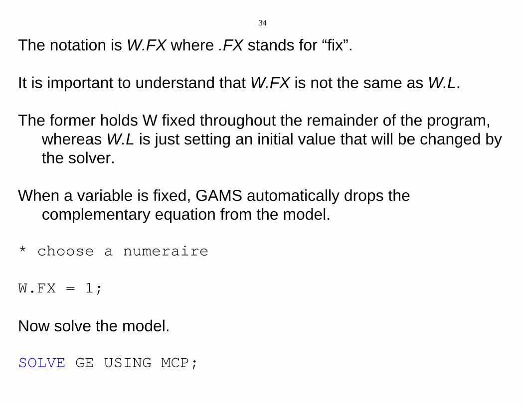
The notation is W.FX where .FX stands for “fix”.
It is important to understand that W.FX is not the same as W.L.
The former holds W fixed throughout the remainder of the program,whereas W.L is just setting an initial value that will be changed bythe solver.
When a variable is fixed, GAMS automatically drops thecomplementary equation from the model.
* choose a numeraire
W.FX = 1;
Now solve the model.
SOLVE GE USING MCP;

35
As a counter-factual, double labor productivity and resolve.
* double labor productivity
ALPHA = 4;SOLVE GE USING MCP;
Here is the solution to the first solve statement. Notice that W.FXshows up as fixing both the upper and lower bounds for W.
LOWER LEVEL UPPER MARGINAL
---- VAR P . 0.500 +INF . ---- VAR X . 200.000 +INF . ---- VAR W 1.000 1.000 1.000 EPS ---- VAR INCOME . 100.000 +INF .

36
Here is the solution to the second solve statement. Doubling of laborproductivity allows twice as much X to be produced from the fixedsupply of labor.
With the wage rate fixed at W = 1, the equilibrium price of X falls inhalf: twice as much X can be purchased from the income from aunit of labor.
LOWER LEVEL UPPER MARGINAL
---- VAR P . 0.250 +INF . ---- VAR X . 400.000 +INF . ---- VAR W 1.000 1.000 1.000 EPS ---- VAR INCOME . 100.000 +INF .

37
In order to appreciate correctly the role of the numeraire, supposeinstead we wanted to choose X as numeraire.
The first thing that we have to do is “unfix” W. This actually requirestwo separate statements, since .FX involves fixing both the lowerand upper bounds of W. Then we set P as numeraire.
W.UP = +INF;W.LO = 0;P.FX = 1;
SOLVE GE USING MCP;
* double labor productivity
ALPHA = 4;SOLVE GE USING MCP;

38
Here are the solutions for the two runs of our model.
LOWER LEVEL UPPER MARGINAL
---- VAR P 1.000 1.000 1.000 EPS ---- VAR X . 200.000 +INF . ---- VAR W . 2.000 +INF . --- VAR INCOME . 200.000 +INF .
LOWER LEVEL UPPER MARGINAL
---- VAR P 1.000 1.000 1.000 EPS ---- VAR X . 400.000 +INF . ---- VAR W . 4.000 +INF . ---- VAR INCOME . 400.000 +INF .

39
In comparing the two alternative choices of numeraire, note that thechoice does not affect the only “real” variable of welfaresignificance, the output of X.
The variables affected are “nominal” variables. Alternatively, onlyrelative prices matter and the “real wage”, W/P is the same undereither choice of numeraire.

C:\jim\COURSES\8858\code-bk 2012\M2-5.gms Monday, January 09, 2012 3:52:24 AM Page 1
$TITLE: M1-5, Structure of a general-equilibrium model* simple (almost trivial) example of a one-good, one-factor,* one-consumer economy
PARAMETERS L B A R labor supply (fixed and inelastic) A L P H A productivity parameter X = ALPHA*L;
LBAR = 100;ALPHA = 2;
NONNEGATIVE VARIABLES P price of X X quantity of X W wage rate I N C O M E income from labor supply;
EQUATIONS Z P R O F I T zeroprofits in X production C M K T C L E A R commodity (X) market clearing L M K T C L E A R labor market clearing C O N S I N C O M E consumer income balance;
C:\jim\COURSES\8858\code-bk 2012\M2-5.gms Monday, January 09, 2012 3:52:24 AM Page 2
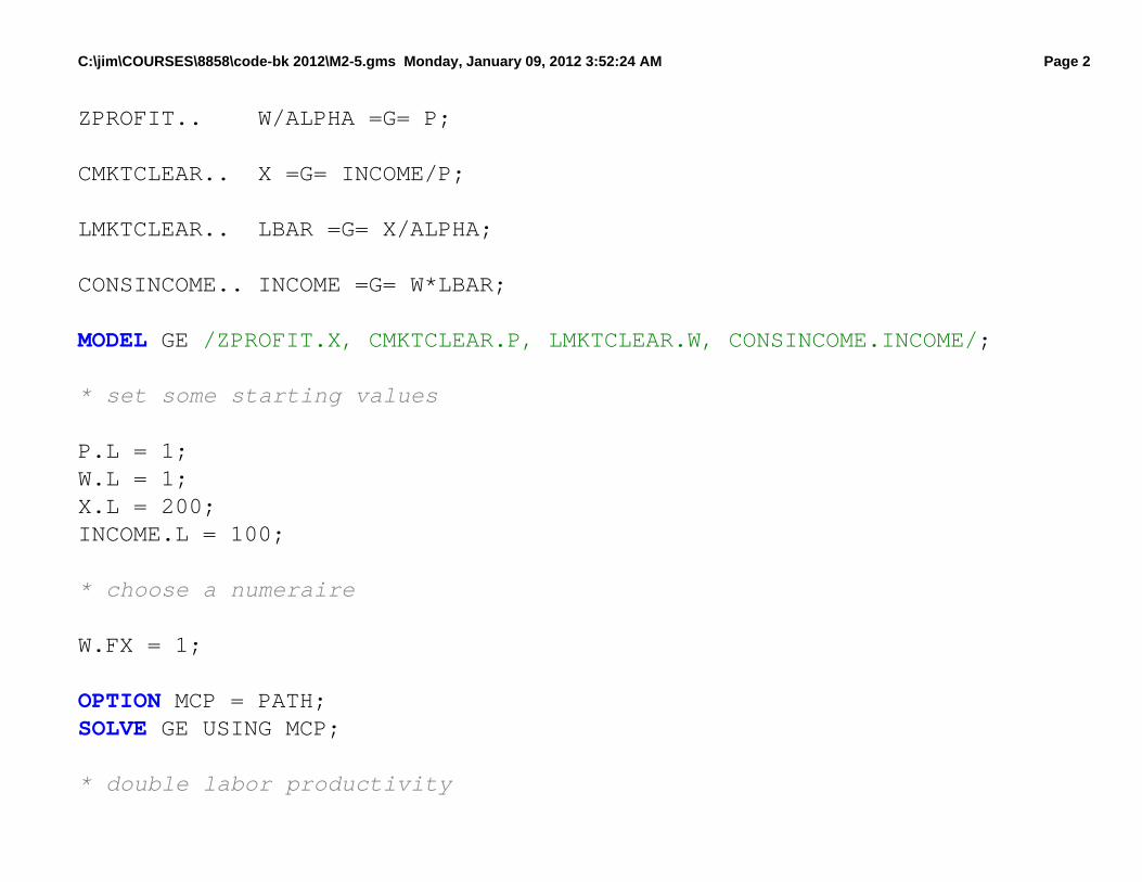
ZPROFIT.. W/ALPHA =G= P;
CMKTCLEAR.. X =G= INCOME/P;
LMKTCLEAR.. LBAR =G= X/ALPHA;
CONSINCOME.. INCOME =G= W*LBAR;
MODEL GE /ZPROFIT.X, CMKTCLEAR.P, LMKTCLEAR.W, CONSINCOME.INCOME/;
* set some starting values
P.L = 1;W.L = 1;X.L = 200;INCOME.L = 100;
* choose a numeraire
W.FX = 1;
OPTION MCP = PATH;SOLVE GE USING MCP;
* double labor productivity

C:\jim\COURSES\8858\code-bk 2012\M2-5.gms Monday, January 09, 2012 3:52:24 AM Page 3
ALPHA = 4;
SOLVE GE USING MCP;
* change numeraire
W.UP = +INF;W.LO = 0;P.FX = 1;
ALPHA = 2;
SOLVE GE USING MCP;
* double labor productivity
ALPHA = 4;
SOLVE GE USING MCP;
$ontextformulated as an NLPthe first theorem of welfare economics says that a competitiveequilibrium is Pareto optimal

C:\jim\COURSES\8858\code-bk 2012\M2-5.gms Monday, January 09, 2012 3:52:24 AM Page 4
in some very simple situation, such as with a single consumerthis means that equilibrium can also be found as the solution to asimple NLP: maximizing utility subject to constraints.$offtext
ALPHA = 2;LBAR = 100;
VARIABLE U;
EQUATIONS OBJECTIVE;
OBJECTIVE.. U =E= X**0.5;
MODEL GE_NLP / OBJECTIVE, ZPROFIT, CMKTCLEAR, LMKTCLEAR, CONSINCOME/;
SOLVE GE_NLP USING NLP MAXIMIZING U;

40
A general formulation of general-equilibrium models
The purpose of this section is to discuss a general formulation.
First, general-equilibrium models consist of activities that transformsome goods and factors into others.
These include outputs of goods from inputs, trade activities thattransform domestic into foreign goods and vice versa, activitiesthat transform leisure into labor supply, and activities thattransform goods into utility (welfare).
Activities are most usefully represented by their dual, or cost-functions.
The conditions for equilibrium: marginal cost for each activity isgreater than or equal to price, complementary variable being theequilibrium quantity or “level” that activity.

41
A quantity variable is complementary to a price equation. Withcompetition and constant returns to scale, these are also referredto as zero profit conditions.
Second, general-equilibrium models consist of market clearingconditions.
A commodity is a general term that includes goods, factor ofproduction, and even utility. Thus X and labor are bothcommodities in our example.
Market clearing conditions require that the supply of a commodity isgreater than or equal to its demand in equilibrium, with thecomplementary variable being the price of that commodity.
A price variable is complementary with a quantity equation.

42
Finally, there are income-balance equations for each “agent” in amodel.
Agents are generally households, but often include a governmentsector, or the owner of a firm in models with imperfectcompetition.
Expenditure (EXP) equals income for each agent.
Let i subscript activities, also referred to as production sectors.
Let j subscript commodities, and let k subscript agents orhouseholds. Our general formulation is then:

43
Inequality Complementary No. ofvariables unknowns
(1) Zero profits MCi $ Pi Activity (quantity) level i i
(2) Market clearing Sj $ Dj Price of commodity j j
(3) Income balance EXPk $ INCOMEk Income k k
The general-equilibrium system then consists of i+j+k inequalities ini+j+k unknowns:
i activity levels, prices of j commodities incomes/expenditures of k agents.
As per our earlier discussion, the price level is indeterminate and oneprice is fixed as a numeraire.
p
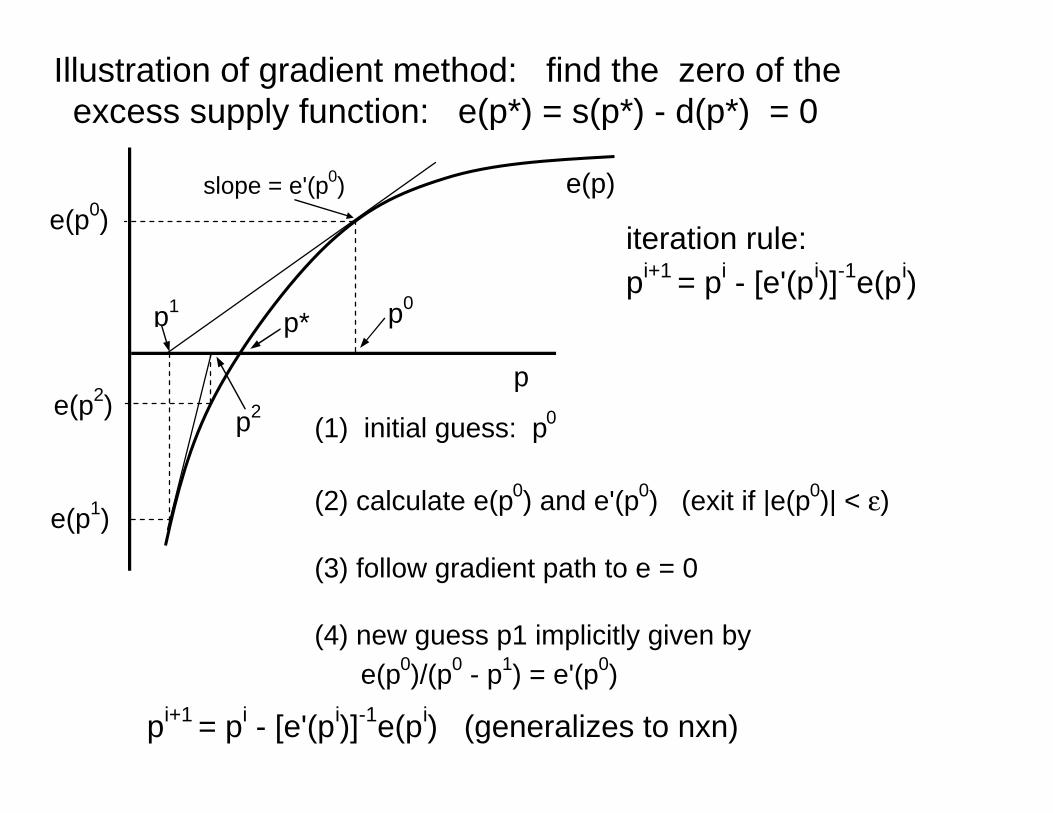
pi+1 = pi - [e'(pi)]-1e(pi) (generalizes to nxn)
p0
(1) initial guess: p0
(2) calculate e(p0) and e'(p0) (exit if |e(p0)| < ε)
(3) follow gradient path to e = 0
(4) new guess p1 implicitly given by e(p0)/(p0 - p1) = e'(p0)
e(p0)
p1
p2e(p2)
Illustration of gradient method: find the zero of the excess supply function: e(p*) = s(p*) - d(p*) = 0
e(p)
e(p1)
iteration rule:pi+1 = pi - [e'(pi)]-1e(pi)
slope = e'(p0)
p*

0.10
0
0.14
0
0.18
0
0.22
0
0.26
0
0.30
0
0.34
0
0.38
0
0.42
0
0.46
0
0.50
0
0.54
0
0.58
0
0.62
0
0.66
0
0.70
0
0.74
0
0.78
0
0.82
0
0.86
0
0.90
0
0.3700.2750.2040.1520.1130.0840.0620.0460.034
0.0260.019
0.014
0.011
0.008
0.006
0.000-0.50
-0.25
0.00
0.25
0.50
0.75
1.00
1.25
1.50
1.75
2.00
Figure 7b: Additional volume of trade from allowing trade in A and C (no trade in B)
Country i's endowment of labor (capital = 1 - labor endowment)
Trad
e C
osts
Add
ed v
olum
e of
trad
e as
a p
ropo
rtion
of r
eal i
ncom
e