economic equilibrium and optimization problems using...
TRANSCRIPT

Economic equilibrium and optimization problems using GAMSNotes 2: from optimization (NLP) to complementarity (MCP)
James R. MarkusenUniversity of Colorado Boulder
Tools of Economic Analysis
(1) Analytical theory models
(2) Econometric estimation and testing.
(3) Simulation modeling - complement to (1) and (2)
(A) greatly extends the reach of theory to problems that areanalytically intractable
(B) extends the economic usefulness of econometrics allowingcounter-factuals using estimation for calibration
1

2
(4) Two ways of formulating economic models
(A) as an constrained optimization problem
(B) as an economic equilibrium problem: square system ofequations/inequalities and unknowns
(5) Limitations of analytical theory
“Many branches of both pure and applied mathematics are in greatneed of computing instruments to break the present stalemate createdby the failure of the purely analytical approach to nonlinear problems”
--- John Von Neumann, 1945

3
Analytical methods quickly become intractable
(1) functions or equation systems have no closed-form solution
(2) large dimensionality (# of equations and unknowns)
(3) correct model consists of non-linear weak inequalities
(6) Responses to difficulties
(1) stick to analytical methods, eliminate difficulties by restrictiveassumptions (even if eliminating the most interesting parts of theproblem)
(2) simulate the model you really want to solve
(3) make an analytical model-of-the-model (e.g., partial equilibrium)and then simulate the richer model

4
(7) Structure of a typical model
Economic models are based on the assumption of optimizingagents: consumers, firms, governments
But, generally the model itself cannot be written as a simpleconstrained optimization problem
Example 1: two households with different preferences/incomesExample 2: two-firm duopoly model
An economic model typically embodies optimization at the level ofthe agent, the model becomes an nxn equilibrium problem

5
Household or firm represented by constrained optimization problem(non-linear programming problem).
Karush-Kuhn-Tucker theorem: converts NLP into a square systemof equations/unknowns, including “slack” variables (Lagraneanmultipliers).
Implicit function theorem => square system can be solved forexplicit functions: endogenous variables each as a function ofsystem parameters.
More often, two-step procedure: KKT functions used to derive cost /expenditure / or indirect utility or profit functions.
Envelop theorem + Shepard’s lemma used to derive goods andfactor demand functions, supply functions, etc.

6
(8) Dimensionality, inequalities, bounded variables
Dimensionality, non-linearity, and simultaneity make models hardto solve analytically past 2 equations in 2 unknowns
Example: 2 factor, 2 good, 2 country Heckscher-Ohlin model
Economics variables are typically bounded (e.g., prices andquantities are non-negative) and economic equilibriumconditions are weak inequalities.
Example: what goods produced, technologies used?Example: what trade links are active in equilibrium?Example: do emissions permits have a positive price?
Economics is often sacrificed to ensure a strictly interior solution.

7
(9) Complementarity: KKT conditions from underlying NLP:
with weak inequality constraints, including non-negativerestrictions on economic variables (prices and quantities)
Equilibrium conditions are weak inequalities
Each inequality is associated with a particular variable, called thecomplementary variable.
If the equation holds as an equality in equilibrium, then thecomplementary variable is generally strictly positive.
If the equation holds as a strict inequality in equilibrium, thecomplementary variable is zero.

8
(10) GAMS solvers: two ways of formulating economic models
(A) NLP: non-linear programming constrained optimization
(B) MCP: mixed complementarity problemsquare system of equations/inequalities and unknownsmatched inequalities and variables
(C) MPEC: mathematical programming with equilibrium constraints: NLP + MCP constraint set
Matching of equations/inequalities and the direction of theinequalities must come from the modeler in accordance witheconomic theory.
9
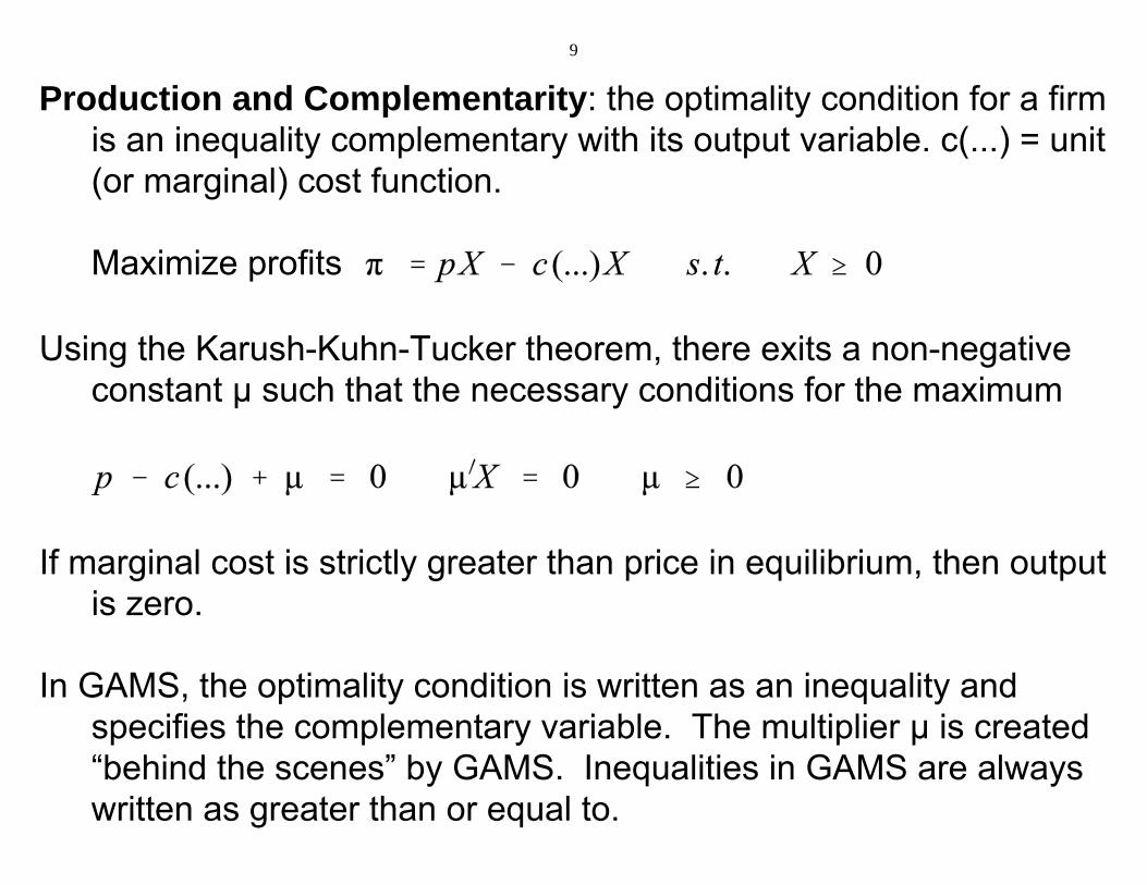
Production and Complementarity: the optimality condition for a firmis an inequality complementary with its output variable. c(...) = unit(or marginal) cost function.
Maximize profits
Using the Karush-Kuhn-Tucker theorem, there exits a non-negativeconstant μ such that the necessary conditions for the maximum
If marginal cost is strictly greater than price in equilibrium, then outputis zero.
In GAMS, the optimality condition is written as an inequality andspecifies the complementary variable. The multiplier μ is created“behind the scenes” by GAMS. Inequalities in GAMS are alwayswritten as greater than or equal to.

10
“the weak inequality is complementary to X”
Though the modeler does not specify the slack variable μ, it willappear in the GAMS output file under the name “marginal”. Thevalue of marginal equals μ.
It follows from the KKT conditions that if the variable X is strictlypositive in the solution, then μ = 0. If X = 0 in the solution, then μis strictly positive.
μ = c(...) - p, and the slack variable μ measures the amount by whichmarginal cost exceeds p in equilibrium.
Alternatively, μ is the difference between the left and right-hand sidesof the weak inequality.

17
Market-Clearing and Complementarity: market clearing requiresthat the value (price times quantity) supplied in a market equal thevalue of demand.
Let D denote the demand for a good while X denotes supply.
there are three possibilities
usual “interior” solution
excess supply, X is a “free good”
violates standard assumption: excessdemand will cause the price to rise
We should model a market-clearing condition as a weak inequalitycomplementary with the price of the good.
“the weak inequality is complementary to p”

18
When GAMS is given this weak inequality and complementaryvariable, it will create equation with a slack variable analogous tothe procedure for the pricing equation.
If the inequality is strict in equilibrium, there is excess supply inequilibrium and the price is zero: X is a free good.
In that case, the auxiliary variable μ, called the “marginal” in theGAMS listing file, has a positive value equal to the supply-demand imbalance in equilibrium: μ = X - D.

19
(12) Simple supply-demand problem illustrating complementarity
Supply and demand model of a single market. Two equations:supply and demand. Two variables: price and quantity.
Economic equilibrium problems are represented as a system of nequations/inequalities in n matched unknowns.
Supply of good X with price P. The supply curve exploits the firm’soptimization decision, P = MC.
MC $ P with the complementarity condition that X $ 0
The price equation is complementary with a quantity variable.

20
Suppose that COST = aX + (b/2)X2.
Marginal cost is then given by MC = a + bX.
a + bX $ P complementary with X $ 0.
Optimizing consumer utility for a given income and prices will yield ademand function of the form X = D(P, M) where M is income.
X $ D(P, M) with the complementary condition that P $ 0.
The quantity equation is complementary with a price variable.
21
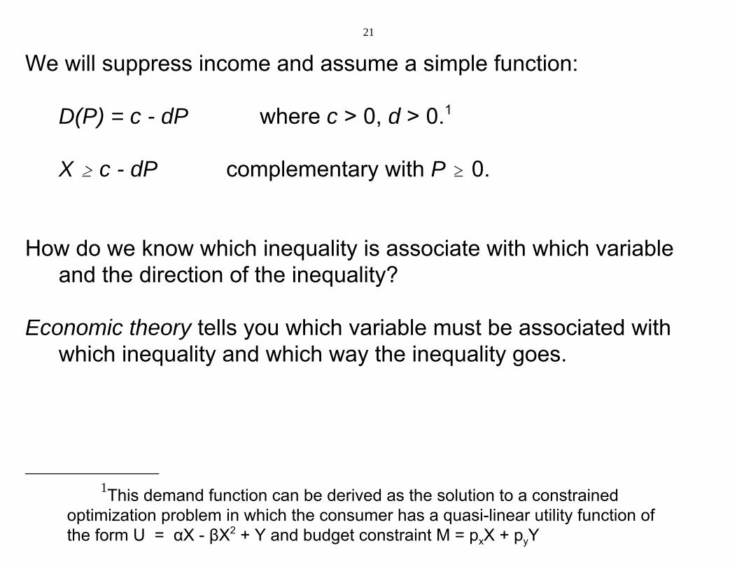
We will suppress income and assume a simple function:
D(P) = c - dP where c > 0, d > 0.1
X $ c - dP complementary with P $ 0.
How do we know which inequality is associate with which variableand the direction of the inequality?
Economic theory tells you which variable must be associated withwhich inequality and which way the inequality goes.
1This demand function can be derived as the solution to a constrainedoptimization problem in which the consumer has a quasi-linear utility function ofthe form U = αX - βX2 + Y and budget constraint M = pxX + pyY

7
Use of slack variables to convert weak inequalities to equalities.
Introduce non-negative variables S1, S2 $ 0
MC(X) - P - S1 = 0
S1*X = 0
X - D(P) - S2 = 0
S2*P = 0
Four equations in four unknowns. Note: S1, S2 give the imbalancesin their corresponding equations in equilibrium.
BUT, there are still the non-negativity constraints to worry about. This is done (I think) in the solution algorithm (discussed later).

Case 1: interior solution
Supply (MC):slope = B
Demand: slope = 1/D
A C
Figure 1: Three outcomes of partial equilibrium example
Case 2: X is too expensive, not produce in equilibrium (X = 0)
Supply (MC)
Demand
A
Case 3: excess supply, X is a free good in equilibrium (P = 0)
Supply (MC)
Demand
A
P
X
P
X
P
X
S1
S2

22
(12) Coding an economic equilibrium problem in GAMS
First, comment statements can be used at the beginning of the code,preceded with a *, in the first column of a line.
$TITLE: M2-1.GMS introductory model using MCP and MPEC* simple supply and demand model
Begin a series of declaration and assignment statements.
PARAMETERS A intercept of supply on the P axis (MC at Q = 0) B slope of supply: this is dP over dQ C demand on the Q axis (demand at P = 0) D (inverse) slope of demand, dQ over dP;
Parameters must be assigned values before the model is solved

23
A = 2; C = 6; B = 1; D = 1;
Declare a list of variables. They are restricted to be non-negative tomake any economic sense, so declaring them as “nonnegativevariables” tells GAMS to set lower bounds of zero.
NONNEGATIVE VARIABLES P price of good X X quantity of good X;
Now we similarly declare a list of equations. Name not otherwise inuse or, of course, a keyword.
EQUATIONS SUPPLY supply relationship (mc cost ge price) DEMAND quantity demanded as a function of price;

24
Specify equations. Format: equation name followed by two periods The equation is written with =G= for “greater than or equal to”.
SUPPLY.. A + B*X =G= P; DEMAND.. X =G= C + D*P;
Declare a model. Keyword model, followed by a model name.
Then a “/” followed by a list of the equation names, each ends with aperiod followed by the name of the complementary variable.
MODEL EQUIL /SUPPLY.X, DEMAND.P/;
Tell GAMS to solve the model and what solver is needed.
SOLVE EQUIL USING MCP;

25
This example uses parameter values which generate an “interiorsolution”, meaning that both X and P are strictly positive.
Case 2: the good, or a particular way to produce or obtain a good(e.g., via imports) is too expensive relative to some alternative:production or trade activity is not used in equilibrium: X = 0.
A = 7;SOLVE EQUIL USING MCP;
Case 3: The final possibility is that a good or factor of production maybe so plentiful that it commands a zero price in equilibrium
A = -7;SOLVE EQUIL USING MCP;

26
(13) Reading the output (file name G1.LST)
GAMS stores four values for a varlable. LOWER and UPPER arebounds on the variables. Declaring a NONNEGATIVE VARIABLEsets the lower bound at 0 (.) and upper bound at +inf.
The LEVEL is the solution value of the variables.
MARGINAL indicates the degree to which the equationcorresponding to the variable is out of equality.
For P (price), the equation is DEMAND and the value of the marginalis supply minus demand.
For X (quantity), the equation is SUPPLY and the value of themarginal is the excess of marginal cost over price.

27
Variables that have positive values in the solution should have zeromarginals.
Variables that have zero values in the solution should have positivemarginals.
Here is the benchmark case.
LOWER LEVEL UPPER MARGINAL
---- VAR P . 4.000 +INF ---- VAR X . 2.000 +INF
28
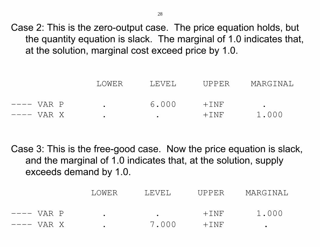
Case 2: This is the zero-output case. The price equation holds, butthe quantity equation is slack. The marginal of 1.0 indicates that,at the solution, marginal cost exceed price by 1.0.
LOWER LEVEL UPPER MARGINAL
---- VAR P . 6.000 +INF . ---- VAR X . . +INF 1.000
Case 3: This is the free-good case. Now the price equation is slack,and the marginal of 1.0 indicates that, at the solution, supplyexceeds demand by 1.0.
LOWER LEVEL UPPER MARGINAL
---- VAR P . . +INF 1.000 ---- VAR X . 7.000 +INF .

29
(14) Example of the use of MPEC: set an endogenous tax rate thatmaximizes tax revenue.
Declare two (unbounded) variables and equations.
VARIABLES T tax rate on marginal cost TREV tax revenue = MC*T*X;
EQUATIONS SUPPLY2 new supply function incorporating endogenous tax OBJ objective function is tax revenue;
OBJ.. TREV =E= (A + B*X)*T*X;
SUPPLY2.. (A + B*X)*(1+T) =G= P;
OPTION MPEC = NLPEC;
MODEL TREVENUE /OBJ, SUPPLY2.X, DEMAND.P/;SOLVE TREVENUE USING MPEC MAXIMIZING TREV;

30
LOWER LEVEL UPPER MARGINAL
---- VAR P . 5.000 +INF EPS ---- VAR X . 1.000 +INF . ---- VAR T -INF 0.667 +INF . ---- VAR TREV -INF 2.000 +INF .

p
pi+1 = pi - [e'(pi)]-1e(pi) (generalizes to nxn)
p0
(1) initial guess: p0
(2) calculate e(p0) and e'(p0) (exit if |e(p0)| < )
(3) follow gradient path to e = 0
(4) new guess p1 implicitly given by e(p0)/(p0 - p1) = e'(p0)
e(p0)
p1
p2e(p2)
Illustration of gradient method: find the zero of the excess supply function: e(p*) = s(p*) - d(p*) = 0
e(p)
e(p1)
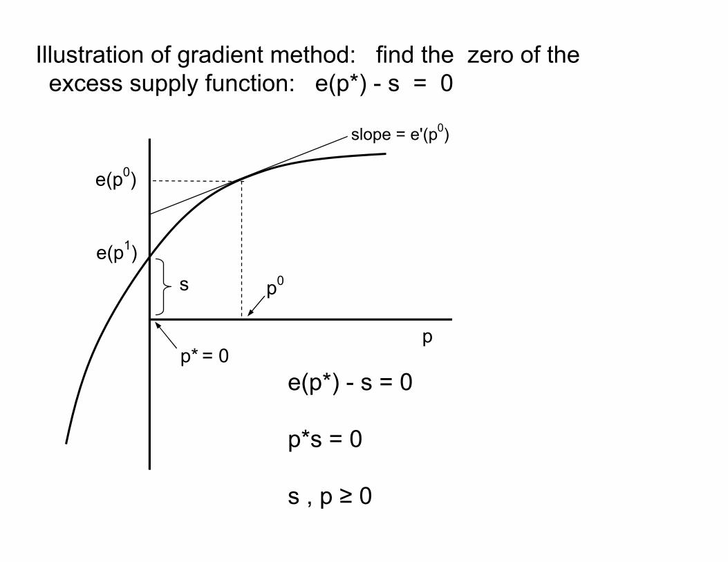
iteration rule:pi+1 = pi - [e'(pi)]-1e(pi)
slope = e'(p0)
p*
p
p0
e(p0)
p* = 0
Illustration of gradient method: find the zero of the excess supply function: e(p*) - s = 0
se(p1)
slope = e'(p0)
e(p*) - s = 0
p*s = 0
s , p ≥ 0

Economic equilibrium and optimization problems using GAMS Continuation of Notes 2
James R. Markusen, University of Colorado, Boulder
Maximization of utility subject to a linear budget constraint
Illustrates the use of the GAMS NLP and MCP solvers
NLP non-linear programmingMCP mixed complementarity problem
Cobb-Douglas utility function with linear budget constraint
Result: C-D exponents are expenditure shares:
25

26
! Option 1: direct solution as an NLP problem
! Option 2a: use KKT to formulated as an MCP, “primal” version
z X1
z X2
z λ
27
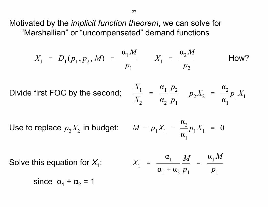
Motivated by the implicit function theorem, we can solve for“Marshallian” or “uncompensated” demand functions
How?
Divide first FOC by the second;
Use to replace in budget:
Solve this equation for X1:
since α1 + α2 = 1

28
Note we can substitute these back into the utility function to get theindirect utility function.
V is termed a value function; that is, it is the maximized value of theLagrangean function for given values of the parameters p1, p2,and M.

29
! Option 2b: use KKT to formulated as an MCP, “dual” version

30
Motivated by the implicit function theorem, we can solve for“Hicksian” or “compensated” demand functions
Divide first FOC by the second;
Substitute this into constraint:

31
Now construct the cost function: the minimum cost of buying U unitsof utility. This is called the “expenditure function” inmicroeconomics.
Substituting from the previous eq
Next, note that the partial derivative of the expenditure function withrespect to a price is the (Hicksian) demand for that good.
Due to Shepard’s lemma, following from the envelop theorem.

32
Envelop theorem: in our case, E is called a value function. Specfically, it is the minimized value of expenditure given theparameters prices and utility.
Consider a function F(Y,β) where Y is a variable(s) and β is aparameter(s). In our case F is the Lagranean function. The valuefunction V is
=> for a given β, Y is chosen such that
(first-order condition) it then follows that

33
In our case,
=>
=0

34
Cost and factor-demand functions for firms.
The expenditure function is just a specific case of a cost function.
It is important for us to note that the exact same procedure allows usto derive a firm’s cost function and, from that, to derive the firm’sdemands for factors of production.
Let X be an output produced from K (capital) and L (labor), whichhave factor prices pk and pl respectively.
The firm’s cost function is given by
(constant returns to scale)

35
Shepard’s lemma then gives the firm’s demands for K and Lconditional on output.
Note that we could also write this as

36
Why should we care?
In even fairly simple general-equilibrium models, we have multipleoptimizing agents: firms and households.
We need to do the optimization at the level of the firm and household,deriving the cost and expenditure functions, and then put all theseparate optimization conditions into a model.
We need to derive market-clearing (supply = demand) conditions forgoods and factors. Here we just need to apply Shepard’s lemmato the cost functions we have just derived to get the demands forgoods and factors.