international trade puzzles: a solution...

INTERNATIONAL TRADE PUZZLES: A SOLUTION LINKINGPRODUCTION AND PREFERENCES*

Justin Caron

Thibault Fally

James R. Markusen

International trade literature tends to focus heavily on the production sideof general equilibrium, leaving us with a number of empirical puzzles. There is,for example, considerably less world trade than predicted by Heckscher-Ohlin-Vanek (HOV) models. Trade among rich countries is higher and trade betweenrich and poor countries lower than suggested by HOV and other supply-driventheories, and trade-to-GDP ratios are higher in rich countries. Our approachfocuses on the relationship between characteristics of goods and services inproduction and characteristics of preferences. In particular, we find a strongand significant positive correlation of more than 45% between a good’s skilled-labor intensity and its income elasticity, even when accounting for trade costsand cross-country price differences. Exploring the implications of this correl-ation for empirical trade puzzles, we find that it can reduce HOV’s overpredic-tion of the variance of the net factor content of trade relative to that in the databy about 60%. Since rich countries are relatively skilled-labor abundant, theyare relatively specialized in consuming the same goods and services thatthey are specialized in producing, and so trade more with one another thanwith poor countries. We also find a positive sector-level correlation betweenincome elasticity and a sector’s tradability, which helps explain the highertrade-to-GDP ratios in high-income relative to low-income countries. JELCodes: F10, F16, O10.

I. Introduction

International trade theory is a general-equilibrium discip-line. Yet it is probably fair to suggest that most of the standardportfolio of research focuses on the production side of generalequilibrium. Price elasticities of demand do play a role in oligop-oly models and, of course, a preference for diversity is importantin all models, not just monopolistic competition. Income

*We thank Donald Davis, Peter Egger, Ana-Cecilia Fieler, Lionel Fontanie,Juan Carlos Hallak, Gordon Hanson, Jerry Hausman, Elhanan Helpman, LarryKarp, Wolfgang Keller, Ethan Ligon, Keith Maskus, Tobias Seidel, InaSimonovska, David Weinstein, anonymous referees, as well as conference andseminar participants at the NBER Summer Institute (ITI), Society of EconomicDynamics, ERWIT CEPR conference, AEA-ASSA Meetings, Midwest TradeMeetings, UC San Diego, Paris School of Economics, Singapore ManagementUniversity, ETH Zurich and the University of Colorado-Boulder for helpfulcomments.

! The Author(s) 2014. Published by Oxford University Press, on behalf of President andFellows of Harvard College. All rights reserved. For Permissions, please email: [email protected] Quarterly Journal of Economics (2014), 1501–1552. doi:10.1093/qje/qju010.Advance Access publication on May 9, 2014.

1501

at University of C

olorado on September 13, 2014

http://qje.oxfordjournals.org/D

ownloaded from

http://qje.oxfordjournals.org/

elasticities of demand are, however, generally assumed to beeither 1 (homothetic preferences) or 0 (so-called quasi-linear pref-erences used in oligopoly models). While nonhomothetic prefer-ences and the role of nonunitary income elasticities were crucialin the work of Linder (1961), subsequent work was limited. Morerecently, we see renewed interest in several strands of literature,including an important one on product quality.

These recent advances notwithstanding, we have a limitedset of theoretical and empirical results regarding possible rela-tionships between the demand and supply sides of general equi-librium; that is, not much is understood about whether certaincharacteristics of goods in production are correlated with othercharacteristics of preferences and demand. The purpose of ourarticle is to investigate such a relationship empirically. In par-ticular, we explore a systematic relationship between factorintensities of goods in production and their correspondingincome elasticities of demand in consumption. The existence ofsuch a relationship can contribute to a number of empirical puz-zles in trade as suggested by Markusen (2013). These include: (i)the mystery of the missing net factor content of trade, (ii) a homebias in consumption, and (iii) large trade volumes among richcountries and small trade volumes between rich and poorcountries.

Our first objective is to estimate the importance of per capitaincome in determining demand patterns. Our results are derivedfrom what we will call ‘‘constant relative income elasticity’’(CRIE) preferences, recently used in Fieler (2011).1 These areintegrated within a general equilibrium model whose supply-side structure is based on an extension of Costinot, Donaldson,and Komunjer (2012) and Eaton and Kortum (2002) with multiplefactors of production and an input-output structure as inCaliendo and Parro (2012). One immediate difficulty we face inthe estimation of preferences is that we have expenditure data,not separate price and quantity data. This is a problem becausetrade costs can imply that goods are relatively cheaper in thecountry where they are produced, so large expenditure shareson home-produced (comparative advantage) goods may be

1. We also provide a discussion of alternative representations of nonhomo-thetic preferences and expressions for expenditure shares across goods: thelinear expenditure system, derived from Stone-Geary preferences, and Deatonand Muellbauer’s almost ideal demand system (Deaton and Muellbauer 1980).

QUARTERLY JOURNAL OF ECONOMICS1502

at University of C



ownloaded from


partly due to trade costs. We solve this problem with a two-stepestimation strategy. First, we use gravity equations to estimatepatterns of comparative advantage and trade costs and show thatthese can be used to compute price index proxies. In the secondstep, we use these indexes to structurally control for price differ-ences and estimate the parameters determining the income elas-ticity of demand. While the estimation of models withnonhomothetic preferences has been considered as challengingin the past, our method is actually quite simple to implementbecause it does not rely on actual price data.2 It is inspired fromRedding and Venables (2004) and would also be consistent with amonopolistic-competition framework yielding gravity equationswithin each sector, as in Redding and Venables (2004) andChaney (2008).3

Our estimations rely on the Global Trade Analysis Project(GTAP) data set, which comprises 94 countries with a widerange of income levels, 56 broad sectors including manufacturingand services, and five factors of production including the disag-gregation of skilled and unskilled labor. This is an excellent dataset for our purposes because it includes harmonized production,input-output, expenditure, and trade data. However, the broadcategories of goods and services make it unsuitable for the dis-cussion of issues related to product quality and within-industryheterogeneity.

Results show that the income elasticity of demand variesconsiderably across goods from different industries. Moreover,it is significantly related both in economic and statistical termsto the skill intensity of a sector, with a correlation of over 50%.This fact has not yet been documented in the literature.4 As ex-pected, accounting for trade costs and supply-side characteristicsreduces this correlation, but it remains large and highly statis-tically significant. The relationship to capital intensity is positivebut much weaker in economic terms and not statistically signifi-cant, consistent with Reimer and Hertel (2010), whereas thecorrelation with natural-resource intensity is negative.

2. As a robustness check, we use actual price data from the InternationalComparison Program.

3. Although the two-step estimation is more robust to misspecifications, wealso propose a one-step estimation imposing additional restrictions on the demandand supply sides.

4. A similar relationship has been emphasized by Verhoogen (2008) regardingquality: the production of high-quality goods tends to involve skilled workers.

INTERNATIONAL TRADE PUZZLES 1503

at University of C



ownloaded from


The estimated parameters are then used to assess the role ofper capita income and nonhomothetic preferences in explainingthe empirical trade puzzles already mentioned. In addition to theincome elasticity/factor intensity relationship, results include thefollowing. First, a systematic relationship between income elas-ticity and skill intensity at the sector level generates a strongcorrelation between the factor content of production and con-sumption across countries. While about half of this correlationcan be explained by trade costs, we find nonhomotheticity to beas important quantitatively. This systematic relationship alsocontributes to solving a large part of the ‘‘missing trade’’ puzzle(Trefler 1995). Standard Heckscher-Ohlin-Vanek (HOV) modelswith homothetic preferences famously predict a much larger vari-ance in the net factor content of trade than what is seen in thedata. We find that nonhomothetic preferences reduce this excessvariance by 60%, even after accounting for trade costs and factorsembodied in intermediate goods.

Second, we illustrate how per capita income and nonhomo-thetic preferences can help us better understand patterns of bi-lateral trade volumes, in particular the low share of tradebetween rich and poor countries (North–South trade). Sincehigh-income countries tend to be relatively abundant in skilledlabor, the correlation between income elasticity and skill inten-sity implies that richer countries tend to consume goods for whichthey have a comparative advantage. Hence, they tend to trademore with one another than with low-income countries. As thismechanism also explains why countries will source a larger shareof their consumption from themselves, nonhomotheticity alsocontributes to explaining why, apart from trade costs, aggregatetrade-to-GDP ratios are not higher than they are (the ‘‘home biaspuzzle’’). Furthermore, we identify a positive sector-level correl-ation between income elasticity and a sector’s tradability, whichcontributes to explaining why rich countries have higher trade-to-GDP ratios than do low-income countries. Overall, allowing fornonhomotheticity largely improves our understanding of the re-lationship between per capita income and openness to trade andexplains part of the home bias puzzle for developing countries.

Our article mainly contributes to two branches of the litera-ture, one focusing on trade volumes and the other focusing on thefactor content of trade. Early papers exploring the relationshipbetween trade volumes and income elasticities are Markusen(1986), Hunter and Markusen (1988), Bergstrand (1990), and


at University of C



ownloaded from


Hunter (1991). A particular focus of this literature is on thevolume of trade in aggregate and among sets of countries andits relationship to a world of identical and homothetic preferencesas generally assumed in traditional trade theory. A general con-clusion of this research is that nonhomotheticity reduces tradevolumes among countries with different per capita income levels,though trade among high-income countries can increase.Matsuyama (2000) uses a competitive Ricardian model to arriveat a similar prediction. There has been a renewed interest in therole of preferences in explaining trade volumes recently, includ-ing Simonovska (2010), Fieler (2011), Bernasconi (2011), andMartinez-Zarzoso and Vollmer (2011).

Closest to our article is Fieler (2011). She shows that aggre-gate trade data between countries are consistent with amodel with two types of goods in which rich countries have acomparative advantage in income-elastic goods. This mechanismgenerates smaller trade flows between rich and poor countries.In Fieler (2011), income-elastic goods are also characterizedby a higher dispersion of productivity and a lower elasticity oftrade to trade costs, which can explain lower trade-to-GDPratios for poorer countries. In our article, we instead examinesector-level data and find evidence of a strong correlation be-tween income elasticity and skill intensity rather than product-ivity dispersion,5 and that this correlation can better explain thelack of trade between poor and rich countries. Another differenceis that Fieler (2011) considers only one factor of production(labor).

Another distinct branch of the literature to which we contrib-ute has examined the net factor content of trade and the predic-tions of the HOV model. As in Trefler (1995) and Davis andWeinstein (2001), most of the attention has been put on thehome bias or trade costs.6 Recent papers, including Cassing and

5. Note that we estimate the productivity dispersion parameter �k by sector,whereas Fieler (2011) estimates it for two broad categories of goods which could bethe aggregation of various types of goods in our model. Simonovska and Waugh(2010) also estimate an aggregate productivity dispersion parameter but find littleevidence that it differs between rich and poor countries.

6. Here, we directly estimate the border effect, or equivalently a home bias inconsumption, in the first-step gravity equation for each industry and control for itwhen we compare homothetic and nonhomothetic preferences.


at University of C



ownloaded from


Nishioka (2009) and Reimer and Hertel (2010), have emphasizedthe role of consumption patterns in explaining part of the‘‘missing trade’’ puzzle, but our results present several contribu-tions. Cassing and Nishioka (2009) show that allowing for richerconsumption patterns yields larger improvements in explainingthe data than allowing for heterogeneous production techniques.They do not however specifically estimate nonhomothetic prefer-ences and cannot examine how much of the missing trade canactually be attributed to nonhomotheticity. Both Cassing andNishioka (2009) and Reimer and Hertel (2010) put an emphasison capital intensity, which is positively but not strongly corre-lated with income elasticity of final demand, but they do not dif-ferentiate skilled from unskilled labor and thus underestimatethe role of nonhomothetic preferences in explaining the missingtrade puzzle.

There are other topic areas where per capita income plays akey role. One is a large and growing literature on product qualitywhere per capita income clearly matters: if a consumer is to buyone unit of a good, consumers with higher incomes buy higherquality goods. In line with Linder (1961), the role of quality dif-ferentiation has been underscored by Hallak (2006, 2010),Khandelwal (2010), Hallak and Schott (2011), and Fajgelbaum,Grossman, and Helpman (2011), among others. In addition, thedistribution of income within a country matters, and a fairly gen-eral result is that higher inequality leads to a higher aggregatedemand for high-quality products. We view this literature as im-portant and most welcome. Note that within-industry realloca-tions only reinforce the mechanisms described in our model. Ifhigh-quality goods are associated with both higher income elasti-cities and stronger skill intensity, the same mechanisms wouldapply for within-industry reallocations as for the between-industry reallocations described herein.7

The rest of the article is organized in three sections. We de-scribe our theoretical framework in Section II, our empiricalstrategy and estimation results in Section III, and the implica-tions for trade patterns and trade puzzles in Section IV.

7. Accounting for within-country inequalities only strengthens our results.We find similar estimates and slightly more variability in income elasticitieswhen using within-country income distribution data by decile (see OnlineAppendix F).


at University of C



ownloaded from

http://qje.oxfordjournals.org/lookup/suppl/doi:10.1093/qje/qju010/-/DC1



II. Theoretical Framework

II.A. Benchmark Model Set-up

1. Demand. The economy is constituted of heterogeneousindustries. In turn, each industry k is composed of a continuumof product varieties indexed by jk2[0,1]. Preferences take theform:

U ¼X

k

�1, kQ�k�1

�k

k ,

where �1,k is a constant (for each industry k) and Qk is a CESaggregate:

Qk ¼

Z 1

jk¼0qðjkÞ

�k�1

�k djk

� � �k�k�1

:

Preferences are identical across countries, but nonhomo-thetic if sk varies across industries. If sk =s, we are back to trad-itional homothetic CES preferences. These preferences are usedin Fieler (2011), with early analyses and applications found inHanoch (1975) and Chao, Kim, and Manne (1982). To the bestof our knowledge, there is no common name attached to thesepreferences, so we refer to them as constant relative income elas-ticity (CRIE) tastes. As shown in Fieler (2011) and below, theratio of income elasticities of demand between goods i and j isgiven by �i

�jand is constant.

The CES price index of goods from industry k in country n is

Pnk ¼ ðR 1

0 pnkðjkÞ1��kdjkÞ

11��k . Given this price index, individual ex-

penditures (PnkQnk) in country n for goods in industry k equal:

xnk ¼ ��kn �2, kðPnkÞ

1��k ,ð1Þ

where �n is the Lagrangian multiplier associated with the budgetconstraint of individuals in country n, and �2, k ¼ ð�1, k

�k�1�kÞ�k . The

Lagrangian �n is determined by the budget constraint: total ex-penditures must equal total income. In general there is no ana-lytical expression for �n.

The income elasticity of demand �nk for goods in industry kand country n equals:

�nk ¼ �k:

Pk0

xnk0Pk0�k0xnk0

:ð2Þ


at University of C



ownloaded from


It is clear from equation (2) that the ratio of the income elas-ticities of any pair of goods k and k0 equals the ratio of their sparameters: �nk

�nk0¼

�k

�k0and is constant across countries. Note that

CRIE preferences (and separable preferences in general) pre-clude any inferior good: the income elasticity of demand isalways positive for any good.8

2. Production. We assume Cobb-Douglas production functionswith constant returns to scale: production depends on factors andbundles of intermediate goods from each industry. We assumethat factors of production are perfectly mobile across sectors butimmobile across countries. We denote by wfn the price of factor f incountry n. Factor intensities for each industry k and factor f aredenoted by �kf . We denote by kh the share of the input bundlesfrom industry h in total costs of industry k (direct input-outputcoefficient), and each input bundle is a CES aggregate of all vari-eties available in this industry (for the sake of exposition weassume that the elasticity of substitution between varieties isthe same as for final goods). Total factor productivity ZikðjkÞvaries by country, industry, and variety.

As common in the trade literature, we assume iceberg trans-port costs dnik� 1 from country i to country n in sector k. The unitcost of supplying variety jk to country n from country i equals:

pnikð jkÞ ¼dnik

Zikð jkÞ

Yf

ðwfiÞ�kfY

h

ðPhiÞkh ,

where Pih is the price index of goods h in country i andPf �kf þ

Ph kh ¼ 1.

There is perfect competition for the supply of each variety jk.Hence, the price of variety jk in country n in industry k equals:

pnkð jkÞ ¼ minifpnikð jkÞg:

We follow Eaton and Kortum (2002) and assume that prod-uctivity Zik( jk) is a random variable with a Frechet distribution.This setting generates gravity within each sector. Productivity is

8. Another notable feature of income elasticities is that they decrease withincome. A larger income induces a larger fraction of expenditures in high-�k indus-tries. Hence, the consumption-weighted average of �k is larger (denominator inexpression (2)), which yields lower income elasticities.


at University of C



ownloaded from


independently drawn in each country i and industry k, with acumulative distribution:

FikðzÞ ¼ exp �ðz=zikÞ��k

� �,

where zik is a productivity shifter reflecting average total factorproductivity (TFP) of country i in sector k. As in Eaton andKortum (2002), �k is related to the inverse of productivity disper-sion across varieties within each sector k. Note that we alsoassume �k > �k � 1 to ensure a well-defined CES price indexwithin each industry.

In the benchmark version of the model, we allow the disper-sion parameter �k to vary across industries. As in Costinot,Donaldson, and Komunjer (2010), we also allow the shift param-eter zik to vary across exporters and industries, keeping a flexiblestructure on the supply side and controlling for any pattern ofRicardian comparative advantage forces at the sector level.

3. Endowments. Each country i is populated by a number Li ofindividuals. The total supply of factor f is fixed in each countryand denoted by Vif. As a first approximation, each person isendowed by

Vif

Liunits of factor Vfi implying no within-country

income inequality. We relax this assumption in OnlineAppendix F and examine how within-country income inequalityaffects our estimates.

II.B. Two Special Cases

Our benchmark specification of the supply side is very flex-ible and allows for several sources of comparative advantage. Wealso propose two more restrictive alternative production specifi-cations to better illustrate the interaction between supply-sidecharacteristics and nonhomotheticity on the demand side.

1. Skill-driven model. In this special case, we impose the dis-persion of productivity 1

� to be equal across all sectors. We alsoimpose the same productivity shifters across all sectors in eachcountry. Additional assumptions in the skill-driven model:

i. Frechet dispersion parameters �k ¼ � are constant acrosssectors.


at University of C



ownloaded from




ii. Productivity shifters zik ¼ zi are constant across all sectorsfor each exporter i.

In this more restrictive version of the model, forces ofRicardian comparative advantage are assumed away. Withcommon �’s and common z’s across sectors, the distribution ofTFP is the same across sectors (for a given country). To betterillustrate the role of skill intensity, we also assume that there areonly two factors of production: unskilled labor and skilled labor,and no intermediate goods.

2. Theta-driven model (Fieler 2011). This particular case rep-licates across industries the assumptions made in Fieler (2011)across (unobserved) types of goods. It allows for variations in �k

across industries but assumes that the technology parameter Ti,defined here as Ti � z�k

ik, is constant across industries. Moreover,as in Fieler (2011), it only considers one factor of production andneglects the differences in factor endowments. Additional as-sumptions in the theta-driven model:

iii. Productivity shifters are given by zik ¼ T1�k

i where Ti is con-stant across sectors for each exporter i.

iv. Labor is only one factor of production f = L.

These assumptions generate a comparative advantage forrich countries (high-T countries) in low-� sectors, that is, sectorswith more dispersed productivity. Following Costinot,Donaldson, and Komunjer (2012), this result derives from theranking in relative productivity shifters:

zik

zi0k¼

Ti

Ti0

� � 1�k

>Ti

Ti0

� � 1�k0

¼zik0

zi0k0

if Ti > Ti0 and �k < �k0 . Since �k also governs the elasticity of tradeto trade costs, Fieler (2011) imposes rich countries to have a com-parative advantage in goods for which there are higher incentivesto trade.

For all versions of the model, equilibrium is characterized bythe same set of market conditions described in the nextsubsection.


at University of C



ownloaded from


II.C. Equilibrium

Equilibrium is defined by the following equations. On thedemand side, total expenditures Dnk of country n in final goodsk simply equals population Ln times individual expenditures asshown in equation (1). This gives:

Dnk ¼ Lnð�nÞ��k�2, kðPnkÞ

1��k ,ð3Þ

where �2, k is an industry constant defined in equation (1). �n isthe Lagrangian multiplier associated with the budget constraint:

Lnen ¼X

k

Dnk,ð4Þ

where en denotes per capita income. Total demand Xnk for goods kin country n is the sum of the demand for final consumption Dnk

and intermediate use:

Xnk ¼ Dnk þX

h

khYnh,ð5Þ

where Ynh refers to total production in sector h.On the supply side, each industry mimics an Eaton and

Kortum (2002) economy. In particular, given the Frechet distri-bution, we obtain a gravity equation for each industry. We followEaton and Kortum (2002) notation with the addition of industrysubscripts. By denoting Xnik the value of trade from country i tocountry n, we obtain:

Xnik ¼SikðdnikÞ

��k

�nkXnk,ð6Þ

where Sik and �nk are defined as follows. The ‘‘supplier effect,’’Sik, is inversely related to the cost of production in country i andindustry k. It depends on the TFP parameter zik, intermediategoods and factor prices:

Sik ¼ z�k

ik

�Yf

ðwfiÞ�kf

��k�Y

h

ðPihÞkh

��k

:ð7Þ

The parameter �k is inversely related to the dispersion ofproductivity within sectors, implying that differences in product-ivity and factor prices across countries have a stronger impact ontrade flows in sectors with higher �k.


at University of C



ownloaded from


In turn, we define �nk as the sum of exporter fixed effectsdeflated by trade costs. �nk plays the same role as the ‘‘inwardmultilateral trade resistance index’’ as in Anderson and vanWincoop (2003):

�nk ¼X

i

SikðdnikÞ��k :ð8Þ

This �nk is actually closely related to the price index, as inEaton and Kortum (2002):

Pnk ¼ �3, kð�nkÞ� 1�k ,ð9Þ

with �3, k ¼ � �kþ1��k�k

� �h i 1�k�1

where � denotes the gamma function.9

Finally, two other market clearing conditions are required todetermine factor prices and income in general equilibrium. Giventhe Cobb-Douglas production function, total income from a par-ticular factor equals the sum of total production weighted by thefactor intensity coefficient �kf . With factor supply Vfi and factorprice wfi for factor f in country i, factor market clearing implies:

Vfiwfi ¼X

k

�kf Yik,ð10Þ

where output equals the sum of outward flows Yik ¼Pn

Xnik. Inturn, per capita income is determined by:

ei ¼1

Li

Xf

Vfiwfi:ð11Þ

By Walras’ law, trade is balanced at equilibrium.The two special cases of the benchmark model share the

same set of equilibrium conditions. Note that Sik takes a morespecific form in each case:

Skill-driven model:

Sik ¼ z�iY

f

ðwfiÞ�kf

!��:ð12Þ

9. Alternatively, we can generalize this model and assume that the elasticity ofsubstitution for intermediate use differs from the elasticity of substitution for finaluse, and depends on the parent industry. This does not affect the elasticity of theprice index with respect to �k as long as the dispersion parameter �k does notdepend on the final use. Differences in elasticities of substitution would then becaptured by the industry fixed effect that we include in our estimation strategy andwould not affect our estimates.


at University of C



ownloaded from


Theta-driven model:

Sik ¼ Tiw��k

i :ð13Þ

II.D. Implications: The Role of Nonhomothetic Preferences

1. Trade partners and volumes of North–South trade. Withnonhomothetic preferences, differences in income per capitaacross countries can result in large differences in consumptionpatterns, even though preferences are assumed identical. In thissection, we illustrate how nonhomotheticity affects trade pat-terns when there is a systematic relationship between preferenceparameters and characteristics of the supply side, for example,factor intensities. Such a relationship is supported by our empir-ical analysis which finds, in particular, a positive correlationacross sectors between skilled-labor intensity and incomeelasticity.

Let us first consider the case in which trade costs areassumed away (dnik = 1). In this case, prices are the same in allcountries and the share of consumption corresponding to importsfrom i in industry k is the same for all importers (country n):Xnik

Dnk¼

SikPjSjk

. Assuming no trade in intermediates and summing

over all industries, total import penetration by country i in coun-try n is:

Xni

Xn¼X

k

SikPj

Sjk

0B@1CA �4, k�

��knP

k0�4, k0�

��k0n

0B@1CA,ð14Þ

where Xn ¼ Lnen is total expenditures in country n, Xni ¼P

k Xnik

is total bilateral trade from country i to n, and �4, k ¼ �2, kP1��k

k isan industry constant incorporating common prices. The first termin parentheses is the share of imports from i in consumption ofk—it reflects the comparative advantage of country i in sector k.The second term corresponds to the share of industry k in finalconsumption of country n.

Aggregate import penetration by country i in country n ob-viously depends on the sectoral composition of both supply anddemand, but the latter has generally been neglected by previouswork. If preferences are homothetic, �k ¼ � is common acrossindustries and import penetration is the same across all


at University of C



ownloaded from


importers n (for a given exporter i). When preferences are non-homothetic (heterogenous �k), exporters with a comparative ad-vantage in high-s industries have a relatively larger penetrationin rich countries (low �n), whereas exporters with a comparativeadvantage in low-s industries have a relatively larger penetra-tion in poor countries (high �n). We show empirically that richcountries have a comparative advantage in high-s (also skill-intensive) industries which can quantitatively explain large dif-ferences in trade volumes across country pairs depending on eachpartner’s per capita income.10

Trade costs provide an alternative explanation as to whyimport penetration varies across markets. On the supply side,proximity reduces unit costs. On the demand side, consumptionmight be biased toward goods produced locally if their price islower (e.g., Saudi Arabia consuming relatively more petroleum).The latter argument requires that the elasticity of substitution belarger than 1. These effects of trade costs can reinforce the pat-terns described here. In our framework, a general expression forthe import penetration of exporter i in market n yields:

Xni

Xn¼X

k

nikshnk ¼X

k

Sikd��k

nik

�nk

!�5, k�

��kn �

�k�1

�k

nkPk0�5, k0�

��k0n �

�k0 �1

�k0

nk0

0BBB@1CCCA,ð15Þ

where �nk ¼P

j Sjkd��k

njk by definition (equation (8)) and

�5, k ¼ �2, k�1��k

3, k is an industry constant. The first term in parenth-

eses corresponds to nik, the share of imports in n from country iin sector k and the second term corresponds to shnk, the share ofsector k in consumption in country n. Import shares and con-sumption shares are both affected by trade costs. In the empiricalsection, we thus need to carefully examine the distinct contribu-tion of trade costs and nonhomotheticity. In addition, we shouldnote that import penetration by exporter i in rich countries mightnot increase with exporter i’s per capita income if competition

10. Formally, if per capita income en increases with n, if Sik is log-supermodular(i.e., countries with higher index i have a comparative advantage in sectors withhigher index k as in Costinot 2009), and if �k increases with k, then Xni is log-

supermodular, which means that Xni

Xni0> Xn0 i

Xn0 i0for any countries n > n0 and i > i0. The

proof follows from Athey (2002) since both Sik and ��kn are log-supermodular.


at University of C



ownloaded from


effects dominate demand effects.11 For instance, a car producermay find it difficult to export cars to Germany because of tradecosts and competition with local producers, even if Germany has arelatively large consumption of cars. Our empirical results, how-ever, indicate that demand effects dominate.

2. Openness and the home bias puzzle. Nonhomothetic prefer-ences can also influence aggregate trade-to-GDP ratios—a keymeasure often used as an indicator of a country’s openness totrade—through at least two channels. First, if high-income coun-tries tend to have a comparative advantage in income-elasticgoods, countries at either end of the income distribution will con-sume larger shares of their own goods than would be predictedunder homothetic preferences. This induces a lower trade-to-GDP ratio and contributes to explaining the home bias puzzle.12

Second, if trade costs are larger for low income-elasticity goods, orif trade is more sensitive to trade costs for such goods (as in Fieler2011), observed aggregate openness will tend to be lower forpoorer countries.

To illustrate these two channels, let us examine �nn the ag-gregate share of goods purchased internally in country n (equal to1 minus the aggregate share of imports over total demand). Itequals:

�nn ¼X

k

nnkshnk,

where nnk �Xnnk

Xnk¼

Snkd��knnkP

iSikd

��knik

is the share of good k purchased from

domestic production. This share only depends on supply-sidecharacteristics (trade costs and the relative cost of producing

goods k). The second term shnk �XnkPk0

Xnk0is the share of good k

in total demand in country n. Let us also denote byav, k ¼

1N

Pn nnk the average share of goods purchased internally

in sector k (inversely related to good k’s tradability).13 Holding

11. Formally, this can arise when ��kn �

�k�1

�k�1

nk is not log-supermodular, even if��k

n is log-supermodular.12. Low levels of international-to-domestic trade flows have been discussed by

McCallum (1995), Anderson and van Wincoop (2003), Yi (2010), among others.13. Note we would have av, k ¼

1N be the same across all goods and countries if

there were no trade costs.


at University of C



ownloaded from


imports shares nik constant within each industry, we can exam-ine the difference in the aggregate demand for domestic goodsimplied by differences between consumption patterns predictedby homothetic and nonhomothetic preferences:

�NHnn � �H

nn¼X

k

nnk�av,k

� shNH

nk � shHnk

� |fflfflfflfflfflfflfflfflfflfflfflfflfflfflfflfflfflfflfflfflfflfflfflfflfflfflfflffl{zfflfflfflfflfflfflfflfflfflfflfflfflfflfflfflfflfflfflfflfflfflfflfflfflfflfflfflffl}

covariance

þX

k

av,k shNHnk � shH

nk

� |fflfflfflfflfflfflfflfflfflfflfflfflfflfflfflfflfflfflffl{zfflfflfflfflfflfflfflfflfflfflfflfflfflfflfflfflfflfflffl}

tradability

,

ð16Þ

where shNHnk and shH

nk denote consumption shares for nonhomo-thetic and homothetic preferences.

If nonhomothetic preferences shift consumption towardgoods in which countries have a comparative advantage (e.g., un-skilled–labor–intensive sectors in low-income countries), the first

‘‘covariance’’ termP

k nnk � av, k

� shNH

nk � shHnk

� should be posi-

tive on average, leading to lower aggregate demand for importedgoods. This illustrates the first channel.

The second term of equation (16) reflects the second mechan-ism described above. If income elasticities are systematically cor-related with tradability av, k across sectors, the second termP

k av, k shNHnk � shH

nk

� can be of a different sign in poor and rich

countries. If trade costs are smaller for income-elastic goods, or ifthe elasticity of trade to trade costs is smaller for income-elasticgoods (as in Fieler 2011), rich countries will tend to consumegoods with smaller av, k. This generates larger trade-to-GDPratios for rich countries than for poor countries.

We show in the empirical section that nonhomothetic prefer-ences play a role through both channels. Note that these mech-anisms reinforce the effect of trade costs. In particular, analternative explanation for low trade-to-GDP in poor countriesis that trade costs are systematically higher in those countries(Waugh 2010). We illustrate quantitatively the role of nonhomo-thetic preferences after accounting for trade costs in gravityequations for each sector.

3. Missing factor content of trade. One reason comparativeadvantage may be related to consumption patterns is that theincome elasticity of demand is correlated with skilled–labor re-quirements. This provides rich countries, which are abundant inskilled labor, a comparative advantage in goods that rich


at University of C



ownloaded from


consumers are more likely to buy. As we describe now, such acorrelation can also shed light on the missing trade puzzle—thefact that the variance in the embodied factor content in nettrade is so low relative to the predictions of the HOV model(Trefler 1995).

Standard HOV models assume homothetic preferences. Thisassumption implies that under costless trade, consumptionshares for each industry are the same in all countries.Accounting for nonhomothetic preferences can yield very differ-ent predictions in terms of factor content of trade. In particular, itcan potentially explain why poor countries trade so little with richcountries (in factor content) even if their endowments differ lar-gely. The intuition is simple. When the income elasticity ofdemand is correlated with skill intensity, consumption in richcountries is biased toward skill-intensive industries, which alsomeans that they are more likely to import from skill-abundantcountries, that is, rich countries. The same intuition would applyto capital if the income elasticity of demand would be correlatedwith capital intensity and if richer countries were relatively moreendowed in capital.

This intuition can be simply illustrated in our framework. Wedefine the factor content of trade Ffn as the value of factor frequired to produce exports minus imports. It equalsFfn ¼

Pk �kf ð

Pi 6¼n Xnik �

Pi 6¼n XinkÞ when there is no intermedi-

ate goods trade and production coefficients �kf are common acrosscountries.14 After simple reformulations, we can decompose Ffn intwo terms:

Ffn ¼ sn

Xk

�Yk�kfYnk

sn�Yk

� 1

� �|fflfflfflfflfflfflfflfflfflfflfflfflfflfflfflfflfflfflfflffl{zfflfflfflfflfflfflfflfflfflfflfflfflfflfflfflfflfflfflfflffl}� sn

Xk

�Yk�kfDnk

sn�Yk

� 1

� �|fflfflfflfflfflfflfflfflfflfflfflfflfflfflfflfflfflfflfflffl{zfflfflfflfflfflfflfflfflfflfflfflfflfflfflfflfflfflfflfflffl}ð17Þ

¼ FHOVfn � FCB

fn ,ð18Þ

where Ynk ¼P

i Xink denotes the value of production of country n

in sector k, �Yk ¼P

n Ynk denotes the value of world production insector k, and sn denotes the share of country n in world GDP. Note

14. The empirical section and the Online Appendix derive additional results toaccount for traded intermediate inputs and production coefficients that differacross countries.


at University of C



ownloaded from



that we define factor content in terms of factor reward instead ofquantities (number of workers or machines).15

In the brackets, the Dnk

sn�Yk

ratio equals the share of consumptionof k in country n relative to the share of consumption of k in the

world. The ratio Ynk

sn�Yk

equals the share of production in sector k in

country n relative to the share of production in sector k in theworld. With homothetic preferences and costless trade, the

second term in brackets would be null ( Dnk

sn�Yk� 1 ¼ 0) and the ex-

pression could be simplified to:

Ffn ¼ FHOVfn ¼ wfnVfn � sn

Xi

wfiVfi:ð19Þ

Under factor price equalization wfn is the same across coun-tries and the expression corresponds to the standard prediction ofthe net factor content trade in the HOV model. This equationstates that the amount of factor f embedded in country n’s exportsshould equal the total value of the supply of factor f in this coun-try minus the value of the world’s supply of this factor adjusted bythe share sn of country n in world GDP.

Equation (19) is violated when preferences are not homo-

thetic and Dnk

sn�Yk� 1 differs from 0. It thus needs to be corrected

by a consumption term FCBfn (where CB stands for consumption

bias). In particular, if relative consumption Dnk

sn�Yk

is positively cor-

related with production Ynk

sn�Yk, then FCB

fn is correlated with FHOVfn and

predicted factor trade is smaller than predicted by models withhomothetic preferences. In the empirical section, we verify thatDnk

sn�Yk

and Ynk

sn�Yk

are indeed strongly correlated across countries and

industries and that FCBfn is correlated with FHOV

fn across countries

and factors.

15. Standard HOV estimation assumes factor price equalization. Under thisassumption, both approaches are equivalent. When FPE is violated, for instance,when factor productivity differs across countries, the predicted factor content has tobe adjusted for such differences if written in terms of factor units (e.g., number ofworkers of machines). No adjustment is necessary if we focus on values, that is,factor supply times factor prices. This approach simplifies the exposition of themain intuitions and better illustrates the contribution of nonhomothetic prefer-ences relative to homothetic preferences without providing too much detail onfactor prices.


at University of C



ownloaded from


Again, trade costs contribute to the positive correlation be-tween supply and demand across industries as well as the lowfactor content of trade as shown by Davis and Weinstein (2001).Additionally, asymmetric trade costs as in Waugh (2010) can ex-plain low levels of trade to and from low-income countries and canpotentially shed some light on the missing trade puzzle. In theempirical section, we disentangle the effect of trade costs andnonhomothetic demand and show that the latter plays an import-ant role. Also, differences in factor requirements across countriesas well as trade in intermediate goods can also partially explainthe missing trade puzzle. In the empirical section, we follow themethodology developed by Trefler and Zhu (2010) to illustrate therole of nonhomotheticity, accounting for more complex verticallinkages.

III. Estimation

The first objective of this section is to detail the two-step es-timation of the benchmark model as well as the one-step estima-tion of the two special cases (skill-driven and theta-drivenmodels), leading to the identification of the parameters determin-ing the income elasticity of demand. The second objective is to testfor a positive correlation between income elasticity and factorintensity.

III.A. Two-Step Estimation of the Benchmark Model

The value of final demand in an industry is determined as inequation (3) or equivalently equation (1) for individual expend-itures xnk ¼

Dnk

Ln. In log, the model yields:

log xnk ¼ ��k: log �n þ log�2, k þ ð1� �kÞ: log Pnk,ð20Þ

where �2, k is a preference parameter that varies across industriesonly. In addition, final demand should satisfy the budget con-straint which determines �n: a higher income per capita is asso-ciated with a smaller Lagrangian multiplier �n.

If there were no trade costs, the price index Pnk would be thesame across countries and could not be distinguished from anindustry fixed effect. If, in richer countries, consumption werelarger in a particular sector relative to other sectors, the esti-mated �k would be larger for this sector. Because trade is notcostless, estimated income elasticities would be biased if we did


at University of C



ownloaded from


not control for the price index Pnk (to capture supply-side charac-teristics). As richer countries have a comparative advantage inskill-intensive industries, the price index is relatively lower inthese industries. Conversely, poor countries have a comparativeadvantage in unskilled–labor–intensive industries and thus havea lower price index in these industries relative to other industries.When the elasticity of substitution between industries is largerthan 1, these differences in price indexes in turn affect the patternsof consumption. If we were not controlling for Pnk, we would over-estimate the income elasticity in skill-intensive sectors.

We proceed in two steps. The main goal of the first step is toobtain a proxy for the price index log Pnk. According to the equi-librium condition (9), log Pnk depends linearly on log �nk whichcan be identified using gravity equations. Then, using the esti-mated price indexes (or equivalently �nk), we can estimate thefinal demand equation (20).

Both steps follow the structure of the benchmark model (gen-eral case) and are also consistent with the two nested models(skill-driven and theta-driven). This two-step procedure esti-mates the supply-side and demand-side parameters separately,and is thus more robust to model misspecifications on either side.In Section III.B, we also develop an alternative one-step estima-tion strategy to estimate the two skill-driven and theta-drivenmodels and exploit additional restrictions that affect both thesupply and demand sides.

1. Step 1: Gravity equation estimation and identification of�nk. By taking the log of trade flows in equation (6), the modelyields:

log Xnik ¼ log Sik � �k log dnik þ log

�Xnk

�nk

�:ð21Þ

We estimate this equation for each sector by including im-porter fixed effects (in place of log Xnk

�nk) and exporter fixed effects

(in place of log Sik) as well as proxies for trade costs dnik. Becausewe do not have data on bilateral transport costs by industry, weassume dnik to be a log-linear combination of various trade costvariables:

log dnik ¼Xvar

�var, kTCvar, ni þ �ATC, ikBi 6¼n,


at University of C



ownloaded from


where TCvar, ni refers to the variables (indexed by var) included inthe gravity equation to capture trade costs between n and i.Following the literature on gravity, we include the log of physicaldistance (including internal distance), a common languagedummy, a colonial link dummy, a border effect dummy (equalto 1 if i 6¼n), a contiguity dummy (equal to 1 if countries i and nshare a common border), a free trade agreement dummy (equal to1 if there is an agreement between countries i and n), a commoncurrency dummy, and a common legal origin dummy (equal to 1 ifi and n have the same legal origin: British, French, German,Scandinavian, or socialist). Parameters �var, k capture the elasti-city of trade costs to each trade cost variable var. They areindexed by k: the effect of each trade cost variable may differacross industries. Notice that all these proxies imply symmetrictrade costs. Following Waugh (2010), we also consider asymmet-ric trade costs (ATCs) by including exporter-specific border effects�ATC, ikBi 6¼n (where Bi 6¼n is a dummy equal to 1 for internationaltrade flows and �ik is an exporter-specific coefficient).

Incorporating the expression for trade costs into the equationfor trade flows (21), we obtain our estimated equation:

Xnik ¼ exp FXik þ FMnk �Xvar

�var, kTCvar, ni � �ATC, ikBi 6¼n þ "Gnik

" #,

ð22Þ

where "Gnik is the error term, FMnk refers to importer fixed effects

and FXik to exporter fixed effects, �ATC, ik ¼ �k�ATC, ik and�var, k ¼ �k�var, k for each trade cost variable var. Note that �k

cannot be directly identified from �var, k using the gravity equa-tion.16 Since all coefficients to be estimated are sector-specific, wecan estimate this gravity equation separately for each sector (as aresult, we do not impose trade balance). Following Santos Silva,and Tenreyro (2006), we estimate gravity using the Poissonpseudo-maximum likelihood estimator (Poisson PML).

The model tells us that importer and exporter fixed effectsFXik and FMnk capture valuable information on Sik and �nk. Wefollow a strategy developed by Redding and Venables (2004) to

16. In Section III.B we examine an alternative specification (theta-drivenmodel) where �var, k are assumed to be constant across sectors and cross-sectoralvariations in trade elasticities can be used to identify differences in �k acrosssectors.


at University of C



ownloaded from


estimate �nk.17 Following equation (8) defining �nk, we use theestimates of log Sik (from cFXik) and �k log dnik (fromP

var �var, kTCvar, ni) to construct a structural proxy for �nk:

�nk ¼X

i

expðcFXik �Xvar

�var, kTCvar, ni � �ATC, ikBi 6¼nÞ:ð23Þ

This constructed �nk varies across industries and countriesin an intuitive way. It is the sum of all potential exporters’ fixedeffect (reflecting unit costs of production) deflated by distance andother trade cost variables. If country n is close to an exporter thathas a comparative advantage in industry k, that is, an exporterassociated with a large exporter fixed effect FXik (large Sik), ourconstructed �nk will be relatively larger for this country, reflect-ing a lower price index of goods from industry k in country n. Notethat �nk also accounts for domestic supply in each industry k(when i = n).18

Such a method would fit various structural frameworks.If our model were based on a Dixit-Stiglitz-Krugman frameworkinstead of Eaton-Kortum, price indexes by importer and industrycould be obtained in the same way. This could account for anendogenous range of available varieties.

2. Step 2: Demand system estimation and identification of �k.The first step estimation gives us an estimate of �nk. From equa-tion (9), we know that the price index Pnk is a log-linear functionof �nk which we can use as a proxy for Pnk on the right-hand sideof equation (20) describing final demand.19 Our estimated equa-tion for per capita final demand is thus:

log xnk ¼ ��k: log �n þ log�5;k þð�k � 1Þ

�klog �nk þ "

Dnk;ð24Þ

17. See also Fally, Paillacar, and Terra (2010) and Head and Mayer (2006). Analternative method uses importer fixed effects and observed total demand to esti-mate �nk. The two methods are actually equivalent when gravity is estimated withPoisson PML, see Fally (2012).

18. Also note that the error term "Gnik is not included in the construction of �nk.

An unobserved shock affecting trade for a specific country pair would not affect �nk.This mitigates potential omitted variable and endogeneity biases jointly affectingtrade relationships and demand patterns.

19. As a robustness check, we estimate the demand equation using actual pricedata instead or in addition to using log �nk (Online Appendix C).


at University of C



ownloaded from



where "Dnk denotes the error term. In each country n, we further

impose the sum of fitted expenditures across sectors to equalobserved total per capita expenditures en:

Xk

exp ��k: log �n þ log�5, k þð�k � 1Þ

�klog �nk

� �¼ en:ð25Þ

We jointly estimate equations (24) and (25) using constrainednonlinear least squares (we minimize the sum of squared errorsð"D

nkÞ2 while imposing both equations (24) and (25) to hold).

Observed variables are the price proxies �nk, individual expend-itures xnk per industry, and total expenditures en.20 Free param-eters to be estimated are the �k, the dispersion parameters �k, theLagrangian multipliers �n, and the industry fixed effects �5;k.

Two normalizations are required. Given the inclusion of in-dustry fixed effects, �n can only be identified up to a constant.21

We thus normalize �USA ¼ 1 for the United States. A similar issuearises for �k, which can be estimated only up to a common multi-plier.22 We thus normalize �TEX ¼ 1 for textiles. Despite this,income elasticities can be derived based on equation (2):

�nk ¼ �k:

Pk0

xnk0Pk0�k0 xnk0

:ð26Þ

Multiplying all �k by the same constant has no effect on esti-mated income elasticities.

This estimation procedure can be seen as a nonlinear leastsquares estimation of equation (24) in which �n is the implicitsolution of equation (25) and thus a function of fitted coefficientsand observed per capita expenditures en.23 Although this estima-tion procedure is consistent with general equilibrium conditions,we show that similar estimates are found when estimating

20. Note that our data are micro-consistent. For each country, we havePk xnk ¼ en.

21. To see this, we can multiply �n by a common multiplier �0 and multiply theindustry fixed effect �k by ð�0Þ�k . Using �n�

0 instead of �n and �kð�0Þ�k instead of �k in

the demand system generates the same expenditures by industry.22. By multiplying �k by a common multiplier �0 and replacing �n by �

1�0

n , weobtain the same demand by industry and the same total expenditures (maintaining�USA ¼ 1).

23. We use the square root of the size of each industry as weights, given that weobtain larger standard errors for smaller industries.


at University of C



ownloaded from


equation (24) either without constraining the sum of fitted ex-penditures to equal observed per capita expenditures en (equation(25)) or in a reduced-form approximation in which log �n isreplaced by a linear function of log en (see Online Appendix B).

The benchmark specification described above identifies �k

and income elasticities solely based on the coefficient associatedwith the Lagrangian �n. The �k parameter also appears in thecoefficient for �nk in equation (24), but the benchmark specifica-tion does not impose any constraint on the coefficient for �nk since�k is a free parameter (we can then identify �k using �k and thecoefficient for �nk). In an alternative estimation, we jointly iden-tify �k from the coefficients on �n and �nk by constraining �k toequal 4 in all sectors.24 This choice of � is close to the Simonovskaand Waugh (2010) estimates of 4.12 and 4.03. Donaldson (forth-coming), Eaton, Kortum, and Kramarz (2011), Costinot,Donaldson, and Komunjer (2012) provide alternative estimatesthat range between 3.6 and 5.2. Alternative values for � yield verysimilar results for income elasticities.

Because �nk is a generated regressor, standard errors on thedemand parameters must explicitly account for errors comingfrom the first-step estimations.25 Because of the nonlinearitiesarising in the computation of �nk, we estimate bootstrap standarderrors by resampling countries (importers) and sectors. For eachbootstrap sample, we reestimate the two steps: gravity and finaldemand. To document the role of errors in the first-step regres-sion in affecting standard errors in income elasticities, we alsoconstruct standard errors by bootstrapping the second step only,neglecting the generated-regressor issue.

III.B. One-Step Estimation of the Two Special Cases

To ensure the robustness of our income elasticity estimates,our benchmark estimation framework allows for any pattern ofcomparative advantage by using exporter-industry fixed effectsin the gravity equation. Two special cases (skill- and theta-drivenmodels) assume more specific patterns of comparative advantage,

24. This fixed-� specification imposes a strong link between income elasticitiesof demand and the coefficient for � in the estimation of equation (24). Note that thelink between price elasticities and income elasticities holds whenever preferencesare separable and is called Pigou’s law (see Deaton and Muellbauer 1980).

25. Pagan (1984) describes biases in estimating standard errors with generatedregressors.


at University of C



ownloaded from



which create explicit links between supply and demand charac-teristics, calling for a one-step estimation with additional cross-restrictions on supply and demand.

1. Skill-driven model. In the skill-driven model, we removeRicardian forces of comparative advantage by imposing commonproductivity across sectors. We also impose common dispersionparameters �k ¼ �. In this model, comparative advantage is solelydriven by differences in skilled–labor intensity across sectors,assuming that skilled and unskilled labor are the only two factorsof production.

Combining expressions for individual final demand (multi-plied by population Ln) and gravity with expression (12) for Sik,we obtain the following specification for the skill-driven model:

log Xnik ¼ � log zi �X

f

��kf log wfi �Xvar

��var, kTCvar, ni

� �k: log�n þ log Ln þ log�5, k þð�k � 1� �Þ

�log �nk þ "

M2nik,

ð27Þ

where �nk satisfies the following constraint:

�nk ¼X

i

exp � log zi�X

f

��kf logwfi�Xvar

��var, kTCvar, ni

" #:ð28Þ

We simultaneously estimate demand-side parameters (�k, �n,and �5, k) and supply-side parameters (factor prices wfk, TFP zi,and trade cost elasticity �var, k).26 Trade flows are regressed usingPoisson PML constrained by equations (27) and (28), and impos-ing the sum of fitted expenditures to equal observed income en (wedo not, however, impose any restrictions on the trade balance).Observed variables include trade flows Xnik, population Ln,income en, trade cost variables TCvar,ni (without exporter-specificborder effects) and skilled– and unskilled–labor intensities �Hk

and �Lk (normalized such that �Hk þ �Lk sum to 1).

26. The GTAP data do not provide information on factor costs. As an externalvalidity check, we verified that countries with a higher schooling years average(Barro and Lee forthcoming update) are associated with a comparative advantagein skill-intensive industries (i.e., larger exporter fixed effects in skill-intensiveindustries).


at University of C



ownloaded from


2. Theta-driven model. In the theta-driven model, differencesin the dispersion parameter �k across sectors are identified byexploiting restrictions on the supply side (patterns of comparativeadvantage and trade costs) and the demand side (the coefficientson �). Following Fieler (2011), we impose the differences in tradecosts elasticities to be driven by differences in �k and assume that�var is constant across sectors. Combining the expression for indi-vidual final demand and gravity with expression (13) for Sik, weobtain our theta-driven model specification:

log Xnik ¼ log Ti � �k log wi �Xvar

�k�varTCvar, ni

� �k: log �n þ log Ln þ log�5, k þð�k � 1� �kÞ

�klog �nk þ "

M3nik:

ð29Þ

with the constraint �nk ¼P

i exp½log Ti � �k log wi �P

var �k�var

TCvar, ni�.Observed variables include trade flows Xnik, population Ln,

income en, and trade costs variables TCvar,ni.27 As in the skill-

driven model and the benchmark estimations, we also imposethe sum of fitted expenditure to equal observed income en. Weestimate the following parameters: �k, �k, the Lagrangian multi-plier �n, wages wi,

28 trade costs elasticities �var , and industry fixedeffects �5, k.

III.C. Data

Our empirical analysis is almost entirely based on the GTAPversion 7 data set (Narayanan and Walmsley 2008). GTAP con-tains consistent and reconciled production, consumption, endow-ment, trade data, and input-output tables for 57 sectors of theeconomy, five production factors, and 94 countries in 2004. Theset of sectors covers both manufacturing and services and the setof countries covers a wide range of per capita income levels.

To estimate gravity equations (22) by industry, we use grossbilateral trade flows from GTAP measured including import tar-iffs, export subsidies, and transport costs (c.i.f.). Demand systemsare estimated over all 94 available countries using final demand

27. As for the skill-driven model, we do not include exporter-specific bordereffects.

28. Wages wi are taken as free parameters, but we obtain similar results usingGDP per capita instead.


at University of C



ownloaded from


values based on the aggregation of private and public expend-itures.29 Some sectors in GTAP are used primarily as intermedi-ates and correspond to extremely low consumption shares of finaldemand. Six sectors for which less than 10% of output goes tofinal demand (coal, oil, gas, ferrous metals, metals n.e.c., andminerals n.e.c.) are assumed to be used exclusively as intermedi-ates and are dropped from the final demand estimations. We alsodrop ‘‘dwellings’’ from our analysis and are left with 50 sectors.

Factor usage data by sector are directly available in GTAPand cover capital, skilled and unskilled labor, land, and othernatural resources. There are, however, some limitations concern-ing the skill decomposition of labor: although the GTAP data setprovides skilled versus unskilled labor usage for all countries,part of this information is extrapolated from a subset ofEuropean countries and six non-European countries (UnitedStates, Canada, Australia, Japan, Taiwan, and South Korea).30

Also, skilled labor is defined on an occupational basis for some ofthese countries (e.g., United States). In most of our analysis, wemeasure factor intensities by the weighted average factor inten-sities across all countries, but our results carry on if our factorintensity measures are solely based on the subset of countriesmentioned above, as shown in Online Appendix E.

Finally, bilateral variables on physical distance, commonlanguage, access to sea, colonial link, and contiguity are obtainedfrom CEPII (www.cepii.fr).31 Dummies for regional trade agree-ment and common currency are from de Sousa (2012).

III.D. Demand System Estimation Results

We focus here on the results from the two-step estimationof the general model. Summary statistics for the two specialcases (skill- and theta-driven models) can be found in OnlineAppendix A. Results from the gravity equation (step 1) are stand-ard and also presented in detail in Online Appendix A. In brief,there is significant variation in the distance and border effectcoefficients across industries. As usually found in the gravity

29. We use trade in final goods computed from GTAP using the proportionalityassumption to estimate the theta- and skill-driven models (equations (27) and (29)).

30. See https://www.gtap.agecon.purdue.edu/resources/download/4183.pdf.31. Distance between two countries is measured as the average distance be-

tween the 25 largest cities in each country weighted by population. Similarly, in-ternal distance within a country is measured as the weighted average of distanceacross each combination of city pairs. See Mayer and Zignago (2011).


at University of C



ownloaded from


www.cepii.fr




https://www.gtap.agecon.purdue.edu/resources/download/4183.pdf


equation literature, the coefficient for distance is on average closeto �1. Coefficients for other trade cost proxies are significant formost industries. The border effect coefficients are large, andallowing them to vary across exporters improves the model’s fitwithout substantially affecting the coefficients for traditionaltrade costs variables such as distance. As in Waugh (2010),these border effects are found to be negatively correlated withexporter per capita income.

We now focus on the final demand estimation (step 2),equation (24). Summary statistics are reported in Table I.Column (1) corresponds to our benchmark specification; column(2) is identical to column (1) except that the border effects used toestimate the �’s are not allowed to vary across exporters (sym-metric trade costs); column (3) is identical to column (1) exceptthat �k is imposed to equal 4 in each sector; column (4) drops theconstraint that fitted expenditures add up to observed total ex-penditures, and column (5) estimates demand without controllingfor cross-country price differences, which is equivalent to impos-ing � ¼ 0.

In all cases, a large part of the variability in the dependentvariable xnk is captured by industry fixed effects, which leads tovery high measures of fit (weighted R2). To better illustrate thecontributions of nonhomotheticity and price differences in ex-plaining demand patterns, we also propose an alternativemetric (partial R2) that measures the increase in fit relative toa model with homothetic preferences and no trade costs (i.e.,imposing common �k ¼ � and � ¼ 0). This reference point alsocorresponds to regressing the log of expenditures on countryand sector fixed effects. The partial R2 in column (1) shows thatour benchmark specification captures 28% of the variability leftunexplained by homothetic preferences without trade costs. Incomparison, homothetic preferences with asymmetric tradecosts yield a partial R2 of 0.18. In column (5), the specificationwith no trade costs (� ¼ 0) shows that nonhomotheticity alonecaptures 15% of the variability left unexplained by homotheticpreferences without trade costs.

The contribution of nonhomotheticity to the fit of demandpatterns is statistically significant: the F-statistics associatedwith imposing common �k’s across industries (sixth row ofTable I) show that homotheticity is clearly rejected in all specifi-cations (all p-values< .001). Similarly, the inclusion of �nk sig-nificantly improves this fit. In the specifications of columns (1) to


at University of C



ownloaded from


(4), the coefficients associated with �nk are found to be jointlysignificant (all p-values< .001). Both the Akaike (AIC) andBayesian (BIC) information criterions favor the specificationthat does not impose individual expenditures to equal observedincome. According to both criterion, the specifications that allowfor nonhomothetic preferences and control for price differences(1–3) are favored to the specification that imposes no prices dif-ferences (5) as well as the specifications (not shown) with homo-thetic preference (with or without trade costs).32

The estimated �k can be used to compute incomeelasticities �nk according to equation (26). Table II displaysestimates from the benchmark model computed using fitted

TABLE I

NON-LINEAR LEAST SQUARES ESTIMATION OF FINAL DEMAND: REGRESSION STATISTICS

(1) (2) (3) (4) (5)

Specification:Benchmark(Asym. TC)

Symmetrictradecosts � ¼ 4

No budgetconstraint � ¼ 0

Correlation �k with 1 0.916 0.913 0.998 0.946benchmark specification

Weighted av. coeff on �nk 0.341 0.510 0.368 0.306 /Correlation log �n with

log per capita income�0.992 �0.982 �0.979 �0.984 �0.999

Correlation �k with �k 0.110 0.201 / 0.167 /�k 75th/25th pctile ratio 2.408 1.912 / 2.412 /

F-stat �k ¼ � 12.58 8.85 4.62 14.70 15.92R2 0.784 0.785 0.775 0.791 0.750Partial R2 0.279 0.281 0.219 0.316 0.150AIC 3.025 3.023 3.047 2.965 3.169BIC 3.360 3.358 3.314 3.300 3.436Parameters 244 244 194 244 194Observations 4,700 4,700 4,700 4,700 4,700

Notes. Constrained non-linear least squares regressions: step 2 of the estimation procedure describedin the text; weighted by industry size (world expenditure by industry); ‘‘Partial R2’’ computed as1� SSE

SSEhomoth ; AIC (Akaike information criterion) computed as lnðSSEn Þ þ

2kn and BIC (Bayesian information

criterion) as lnðSSEn Þ þ

k lnðnÞn , where n is the number of observations and k is the number of parameters.

32. The values for AIC and BIC under homothetic preferences are 3.310 and3.508 without controlling for prices and 3.136 and 3.403 if controlling for them. AICyields a larger gap between homothetic and nonhomothetic preferences as it puts asmaller penalty on models with more degrees of freedom.


at University of C



ownloaded from


TABLE II

ESTIMATED INCOME ELASTICITY BY SECTOR

GTAPcode Sector name

Incomeelast.

Std.error

Skillintensity

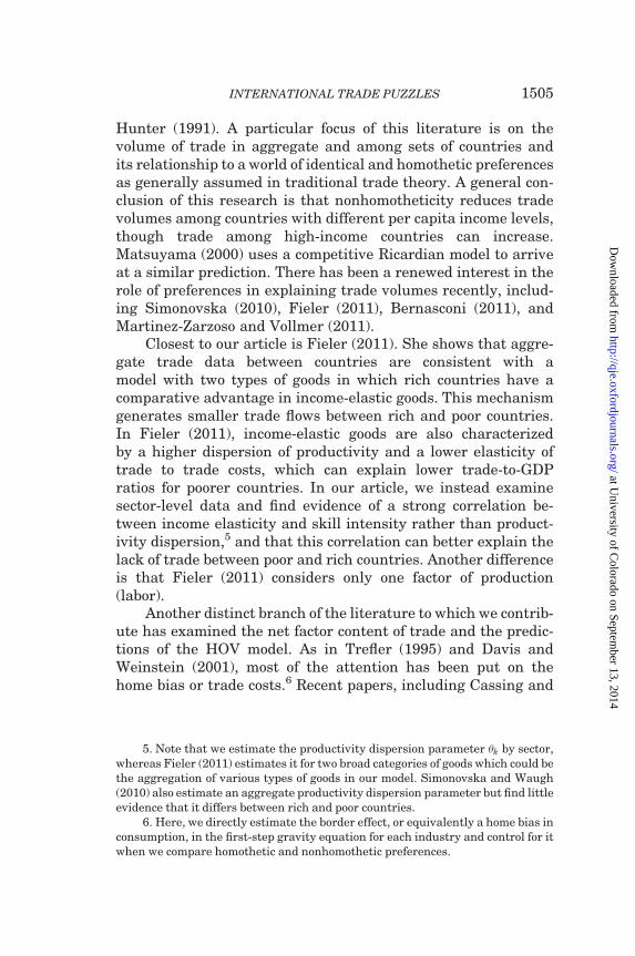
gro Cereal grains nec 0.110* 0.133 0.135pdr Paddy rice 0.254* 0.199 0.061pcr Processed rice 0.352* 0.113 0.130c_b Sugar cane, sugar beet 0.433* 0.233 0.091oap Animal products nec 0.444* 0.098 0.132ctl Bovine cattle, sheep and goats, horses 0.458* 0.137 0.164vol Vegetable oils and fats 0.545* 0.063 0.217sgr Sugar 0.588* 0.085 0.221frs Forestry 0.623* 0.121 0.118v_f Vegetables, fruit, nuts 0.640* 0.136 0.095p_c Petroleum, coal products 0.664* 0.052 0.313b_t Beverages and tobacco products 0.667* 0.079 0.297tex Textiles 0.707* 0.064 0.231ofd Food products nec 0.777* 0.063 0.268mil Dairy products 0.826* 0.077 0.248ely Electricity 0.848* 0.073 0.372nmm Mineral products nec 0.874 0.097 0.281crp Chemical, rubber, plastic products 0.880 0.067 0.356cns Construction 0.880 0.061 0.294wht Wheat 0.883 0.202 0.117fsh Fishing 0.886 0.139 0.124osd Oil seeds 0.889 0.194 0.119ocr Crops nec 0.893 0.144 0.115atp Air transport 0.929 0.070 0.313wtp Water transport 0.932 0.100 0.299ome Machinery and equipment nec 0.938 0.066 0.372lum Wood products 0.970 0.103 0.248otn Transport equipment nec 0.981 0.076 0.343lea Leather products 0.981 0.066 0.212otp Transport nec 0.990 0.074 0.296fmp Metal products 0.992 0.077 0.297cmt Bovine meat products 1.023 0.078 0.238osg Public Administration and services 1.033 0.049 0.503mvh Motor vehicles and parts 1.034 0.066 0.341wtr Water 1.039 0.087 0.378ppp Paper products, publishing 1.044 0.093 0.340omt Meat products nec 1.052 0.096 0.233wap Wearing apparel 1.057 0.069 0.247ros Recreational and other services 1.075 0.067 0.475ele Electronic equipment 1.094 0.070 0.358omf Manufactures nec 1.095 0.065 0.279trd Trade 1.106 0.070 0.308rmk Raw milk 1.118 0.145 0.152cmn Communication 1.152* 0.078 0.485obs Business services nec 1.324* 0.059 0.504ofi Financial services nec 1.331* 0.090 0.546pfb Plant-based fibers 1.339* 0.193 0.167isr Insurance 1.392* 0.104 0.533wol Wool, silk-worm cocoons 1.426* 0.177 0.089gdt Gas manufacture, distribution 2.221* 0.260 0.362

Notes. Estimates based on the benchmark specification; income elasticities evaluated using mediancountry expenditure shares; bootstrapped standard errors (500 draws); *denotes 5% significance (differ-ence from unity); skill intensity based on total requirements.


at University of C



ownloaded from


median-income-country expenditure shares as weights.33 Esti-mates range from 0.110 for cereal grains to 2.221 for gas manu-facture and distribution with a clear dominance of agriculturalsectors at the low end and service sectors at the high end. Half ofthe estimates are significantly different from 1 (at 95%). Stan-dard errors are on average equal to 0.102 when both estimationsteps are run for each bootstrap. Only accounting for errors in thesecond step, that is, assuming �nk to be an error-free variable,yields an average standard error of 0.094. This small differencesuggests that measurement errors stemming from the first stepare small. A third alternative is to construct bootstrap by resam-pling countries but not sectors.34 This method again yields verysimilar standard errors.

The distribution of estimated income elasticities is quitesimilar across specifications (see Figure I). In particular, wefind that the choice of �k does not substantially affect estimatesof �k. As shown in Table I, the correlation between the estimated�k in other specifications and those of the benchmark specificationis always above 85%. This is also the correlation between incomeelasticities among specifications because income elasticities areproportional to �k. Sectors where income elasticities vary themost across specifications are actually the smallest ones (suchas wool), and weighing this correlation by final demand yieldslarger correlation estimates in all cases.

For robustness, our estimated income elasticities are com-pared with estimates based on AIDS and LES, two more standarddemand systems, and are found to be well correlated (OnlineAppendix E). In addition, we propose a reduced-form approxima-tion of our benchmark equation (Online Appendix B). Since theLagrangian multiplier �n is highly negatively correlated with percapita income (in log), we can approximate income elasticitiesusing coefficients on log per capita income instead of the log ofthe Lagrangian and find similar estimates.

In the benchmark specification, we can also use our esti-mates of �k to examine the differences in �k across sectors impliedby the estimated coefficient on �nk. Doing so, we find a positive

33. With CRIE preferences, the ratio of income elasticities between two sectorsdoes not depend on the choice of the reference country.

34. This ‘‘block-bootstrap’’ approach accounts for clusters if errors are corre-lated across industries for each importer.


at University of C



ownloaded from





0.5

11.

52

2.5

Est

imat

ed In

com

e el

astic

ities

Gas

man

ufac

ture

, dis

trib

utio

nW

ool,

silk

−w

orm

coc

oons

Insu

ranc

eP

lant

−ba

sed

fiber

sF

inan

cial

ser

vice

s ne

cB

usin

ess

serv

ices

nec

Com

mun

icat

ion

Raw

milk

Tra

deM

anuf

actu

res

nec

Ele

ctro

nic

equi

pmen

tR

ecre

atio

nal a

nd o

ther

srv

Wea

ring

appa

rel

Mea

t pro

duct

s ne

cP

aper

pro

duct

s, p

ublis

hing

Wat

erM

otor

veh

icle

s an

d pa

rts

Pub

lic s

pend

ing

Bov

ine

mea

t pro

duct

sM

etal

pro

duct

sT

rans

port

nec

Leat

her

prod

ucts

Tra

nspo

rt e

quip

men

t nec

Woo

d pr

oduc

tsM

achi

nery

and

equ

ipm

ent n

ecW

ater

tran

spor

tA

ir tr

ansp

ort

Cro

ps n

ecO

il se

eds

Fis

hing

Whe

atC

onst

ruct

ion

Che

mic

al, r

ubbe

r, p

last

icM

iner

al p

rodu

cts

nec

Ele

ctric

ityD

airy

pro

duct

sF

ood

prod

ucts

nec

Tex

tiles

Bev

erag

es a

nd to

bacc

oP

etro

leum

, coa

l pro

duct

sV

eget

able

s, fr

uit,

nuts

For

estr

yS

ugar

Veg

etab

le o

ils a

nd fa

tsC

attle

, she

ep, g

oats

, hor

ses

Ani

mal

pro

duct

s ne

cS

ugar

can

e, s

ugar

bee

tP

roce

ssed

ric

eP

addy

ric

eC

erea

l gra

ins

nec

Ben

chm

ark

The

ta=

4

Phi

=0

FIG

UR

EI

Inco

me

Ela

stic

ity

Est

imate

sacr

oss

Sp

ecifi

cati

ons


at University of C



ownloaded from


but not statistically significant correlation between �k and �k

(fourth line of Table I).Alternatively, we can also use the skill- and theta-driven

models to estimate �k and �k across sectors. While we leave forOnline Appendix A the summary statistics of the estimation ofeach special case, note that we find the correlation of the esti-mated �k with our benchmark estimates to be 60% for the skill-driven model and 61% for the theta-driven model. Moreover, thecorrelation between �k and �k in the theta-driven model is nega-tive at �0.16 but not significant at the 10% level.

III.E. Correlation with Factor Intensities

We now investigate the relationship between income elasti-cities and factor intensities across sectors. Although the implica-tions of such a relationship will be best illustrated in Section IVwe demonstrate its significance through simple correlations.Table III reports correlation coefficients between skill intensityand income elasticity, or, in columns (2) and (4), the beta coeffi-cients associated with each intensity parameter in regressions ofincome elasticity on several factor intensities. It displays stand-ard errors constructed by resampling importers and sectors in allsteps of the estimation: the two steps required to estimate incomeelasticities as well as the correlation with factor intensities.35

Our measures of factor intensity correspond to the ratio ofskilled labor, capital, or natural resources (including land) tototal labor input. They are computed including the factor usageembedded in the intermediate sectors used in each sector’s pro-duction, based on data pooled across all countries for greater pre-cision. Online Appendix E shows that our results are robust todifferent measures of factor intensities. Table III reports esti-mates resulting from CRIE preferences, while alternative

35. We compare them to bootstrapped standard errors resulting fromtaking the�’s as perfectly measured and find similar results: for example, the estimate incolumn (1) is 0.121 instead of 0.120. Alternatively, we have computed standarderrors on the correlation coefficient using a feasible generalized least squares re-gression in which the bootstrapped standard errors from the non-linear leastsquares estimations of income elasticities are used to construct weights (seeLewis and Linzer 2005). These lead to standard error estimates (0.113) that arevery close to both those resulting from the full bootstrapping (0.120) and to thoseresulting from a simple robust OLS regression of income elasticity on skill intensity(0.123). Thesimilarity betweenestimates suggests that the bias caused bythe use ofgenerated variables is small.


at University of C



ownloaded from




TA

BL

EII

I

CO

RR

EL

AT

ION

BE

TW

EE

NIN

CO

ME

EL

AS

TIC

ITY

AN

DS

KIL

LIN

TE

NS

ITY

(1)

(2)

(3)

(4)

(5)

(6)

(7)

(8)

Dep

end

ent

var.

:In

com

eel

ast

icit

y

Sp

ecifi

cati

on:

Ben

chm

ark

(Asy

m.

TC

)B

ench

mark

(Asy

m.

TC

)S

ym

met

ric

trad

eco

sts

Sym

met

ric

trad

eco

sts

�¼

4�¼

0E

xcl

.se

rvic

esE

xcl

.se

rvic

es

Sk

ill

inte

nsi

ty0.5

23

0.5

31

0.4

96

0.4

65

0.5

13

0.6

51

0.3

61

0.4

90

[0.1

20]*

*[0

.158]*

*[0

.118]*

*[0

.163]*

*[0

.161]*

*[0

.088]*

*[0

.181]*

[0.2

31]*

Cap

ital

inte

nsi

ty0.0

68

0.0

62

�0.3

85

[0.2

68]

[0.2

33]

[0.3

56]

Nat.

res.

inte

nsi

ty�

0.0

05

�0.2

03

0.2

13

[0.1

80]

[0.1

45]

[0.2

90]

Obs.

(sec

tors

)50

50

50

50

50

50

42

42

Not

es.

Dep

end

ent

vari

able

:in

com

eel

ast

icit

yby

sect

orev

alu

ate

dat

med

ian

-cou

ntr

yin

com

e;‘‘N

at.

rces

.in

t.’’:

natu

ral

reso

urc

esin

ten

sity

;bet

aco

effi

cien

ts;

boo

tstr

ap

stan

dard

erro

rsin

bra

cket

s(5

00

dra

ws)

;*

sign

ifica

nt

at

5%

;**

sign

ifica

nt

at

1%

.


at University of C



ownloaded from


demand systems are examined in Online Appendix D. The correl-ation with skill intensity is also illustrated in Figure II.

We find that skill intensity is positively and significantlycorrelated with income elasticity, natural resources intensity isweakly negatively correlated, and capital intensity exhibits aweakly positive correlation. As expected, the correlation withskill intensity diminishes if we account for trade costs and controlfor differences in price indexes. This can be seen by comparingcolumn (1) versus (6) in Table III. This correlation remains how-ever particularly large and around 50% in most specifications.

This correlation is not driven by sectors that contribute littleto final demand: it is even stronger when we weight observationsby world final consumption in each industry (not shown). Part ofthis large correlation can be explained by the composition of con-sumption into services versus manufacturing industries, with theformer being generally associated with a larger income elasticity.However, columns (7) and (8) of Table III show that the correl-ation remains high even after excluding service industries. Inthat case, the correlation is significant at 5% (column (7)) and1% (column (8)) depending on whether we control for capital in-tensity and natural resources intensity. We also test the correl-ation between skill intensity and income elasticity usingestimates from the two special cases (skill- and theta-drivenmodels) where we impose additional constraints on the supplyside. We find even stronger correlations: 65.3% for the skill-driven model and 71.6% for the theta-driven model.36

It is interesting to note that capital intensity would otherwisebe positively correlated with income elasticity, as found byReimer and Hertel (2010), but this correlation is not as large asfor skill intensity (less than 10% in most specifications) and notrobust to controlling for skill intensity as shown in columns (2)and (4) of Table III.

These results imply a large correlation between per capitaincome and final demand in skill-intensive sectors. We emphasizethe demand side. One may be worried, however, that theseresults are driven by differences in skill endowment across coun-tries rather than differences in per capita income. In the GTAP

36. Note that the theta-driven model assumes that there is only one factor ofproduction. It shows, however, that alternative estimates of income elasticities arestill correlated with observed skill intensity across sectors.


at University of C



ownloaded from



data, the fraction of payment to skilled labor is indeed correlatedat 88% with log per capita income.37 To check the robustness ofour results with respect to differences in education, we reesti-mated income elasticities for subsets of countries with smallervariations in skilled–labor endowment (and still large variationsin per capita income). If we restrict the set of countries to thosewithin the interquartile range in skilled-labor endowments, thecorrelation between estimated income elasticities and skill inten-sity remains very high for the main specifications (above 40%)and the correlation between per capita income and education issensibly lower. A more extreme exercise is to select specificgroups of countries where the correlation between income andeducation becomes zero by construction. In these cases we findagain very large correlations between skill intensity and (reesti-mated) income elasticity, showing that our main results are notdriven by differences in education across countries.

atp

b_t

c_b

cmn

cns crp

ctl

ele

ely

fmp

frs

fsh

gdt

gro

isr

lea lum

mil

mvh

nmm

oap

obs

ofd

ofi

ome

omfosg

otn

p_c

pcrpdr

pfb

rmkros

sgr

tex

trd

v_fvol

wap

wol

wtr

0.5

11.

52

2.5

Est

imat

ed In

com

e el

astic

ities

0 .2 .4 .6

Skill intensity

FIGURE II

Income Elasticity and Skill Intensity Correlation

Income elasticities are evaluated at median country expenditure shares(benchmark spec.).

37. Similarly, the correlation between average schooling years and per capitaincome is very high: 74.7% using data from Barro and Lee (2012 update).


at University of C



ownloaded from


IV. Implications for Trade Puzzles

In this section, we use our estimates to illustrate the impli-cations of nonhomothetic preferences for: (i) the correlation be-tween consumption and production, (ii) the missing trade puzzlein factor content, (iii) the volume of trade flows between rich andpoor countries, and (iv) aggregate trade-to-GDP ratios. We inves-tigate these topics using our benchmark specification (incorpor-ating asymmetric trade costs) and an identical model withhomothetic preferences as a point of reference. Items (iii) and(iv) are also investigated using the two special cases (skill- andtheta-driven models) to distinguish the roles of differences infactor intensities and differences in dispersions of productivity.

IV.A. Consumption patterns and Missing Trade

The correlation between skill intensity and income elasticityimplies that the factor content of consumption varies systematic-ally with income. In Figure III, we plot per capita income (in log)against a measure of the relative skilled-labor content ofconsumption: P

k

�HkDnkPk

ð�Lk þ �HkÞDnk

,ð30Þ

where �Hk and �Lk are defined as the skilled–labor and unskilled–labor intensity of production (using average of total requirementsacross all countries). We define final demand by using eitheractual consumption or fitted consumption Dnk with different as-sumptions. With homothetic preferences and no trade costs, ex-pression (30) would be the same for all countries. Trade costs(including asymmetric trade costs) already explain part of thevariations in the factor content of consumption: rich countriestend to spend more on skilled–labor–intensive industries, evenif preferences are homothetic, because goods from these indus-tries are relatively cheaper in these countries. However, we cansee in Figure III that an even better fit is obtained when nonho-mothetic preferences are allowed on top of trade costs.

As shown in Figure IV, rich countries also tend to specializein skill-intensive sectors. This generates a correlation betweenrelative specializations in consumption and production, which

we illustrate by looking at the relationship between Vnk

sn�Vk

and Dnk

sn�Yk


at University of C



ownloaded from


in the first row of Table IV. The term Vnk

sn�Vk

reflects actual value-

added in sector k of country n relative to world total value-addedin sector k multiplied by country n’s share of world expenditures.

The second term Dnk

sn�Yk

corresponds to the relative specialization in

consumption, which is computed using fitted final demand Dnk

from our second-stage estimates including trade costs (both sym-metric and asymmetric) in columns (1) to (3) and using observedconsumption Dnk in column (4). Note that if preferences werehomothetic and there were no trade costs, as is assumed in stand-ard Heckscher-Ohlin models, the correlation would be null asconsumption patterns would be the same across all countries

and Dnk

sn�Yk

¼ 1. In columns (1) and (2), we find a positive correlation

between consumption and production even if preferences areassumed to be homothetic. The estimated correlation across coun-tries and industries is 34% and 37% (with and without asymmet-ric border effects) and significantly positive at 1%. Column (3)shows that this correlation increases to 49% if we account for

BGD

BRA

BWA CHE

CHN

COL

ETH

FIN

HKG

IND

JPN

KGZ

KOR

LAO

LUX

MDG

MEX

MMR

MOZ

MWI

NZL

PAN

PRT

PRY

SEN

SGPSVK

THA TUR

TZA

UGA

USA

VNM

ZWE

BGDBRA

BWA

CHE

CHN

COL

ETH

FIN

HKG

IND

JPN

KGZ

KOR

LAO

LUX

MDG

MEX

MMR

MOZMWI

NZL

PAN

PRT

PRY

SENSGP

SVK

THATUR

TZA

UGA

USA

VNM

ZWE

.15

.2.2

5.3

Ave

rage

ski

lled

labo

r co

nten

t of c

onsu

mpt

ion

4 6 8 10 12

Log per−capita expenditure

Non−homoth. slope=0.013 (s.e. 0.001)Homothetic slope=0.007 (s.e. 0.001)Data slope=0.015 (s.e. 0.001)

FIGURE III

Skilled–Labor Content of Consumption and Per Capita Income


at University of C



ownloaded from


both nonhomothetic preferences and trade costs. This value iscloser to the 62% correlation observed in the data (column (4)).

1. Missing trade in factor content: slope and variance tests. Apositive correlation between income elasticity and skill intensitygenerates not only a correlation between supply and demand butalso a smaller factor content trade compared to the homothetic case.

As described in Section II.D.3, the predicted factor content oftrade (PFCT) can be expressed as the difference between stand-

ard HOV PFCT, denoted FHOVnf , and a consumption bias term

denoted FCBnf (see equation (17)). Assuming constant require-

ments coefficients �kf across countries, we impute FHOVnf using

production data and FCBnf using either fitted final demand (col-

umns (1) to (3)) or actual consumption (column (4)).38 This

AUS

AZE

BEL

BGD

BLR

BOL

BRA

BWA

CHE

CHL

CHN

COL

DNK

ECU

ETH

GBR

GRC

GTM

HRV

IND

KHM

KOR

LAO

LTU

LUX

LVAMAR

MDG

MEX

MMR

MUS

MWI

NGA

NOR

NZL

PAK

PRT

PRY

SVN

THA

TZA

UGA

URY

USA

VEN

VNM

ZAF

ZMBZWE AUS

AZE

BEL

BGD

BLR

BOL

BRA

BWA

CHE

CHL

CHN

COL

DNK

ECU

ETH

GBR

GRC

GTM

HRV

IND

KHM

KOR

LAO LTU

LUX

LVA

MAR

MDG

MEX

MMR

MUS

MWI

NGA NOR

NZLPAK

PRT

PRY

SVN

THA

TZAUGA

URY

USA

VEN

VNM

ZAF

ZMB

ZWE

.05

.1.1

5.2

.25

.3A

vera

ge s

kille

d la

bor

cont

ent o

f pro

duct

ion

4 6 8 10 12

Log per−capita expenditure

Output slope=0.018 (s.e. 0.001)Exports slope=0.017 (s.e. 0.002)

FIGURE IV

Skilled–Labor Content of Production and Exports against Per Capita Income

38. For this correlation, as well as the slope and variance tests, all observationsare scaled by ðsn

Pi wif Vif Þ

1=2 to adjust for heteroskedasticity. Note also that allvariables are in value terms (e.g., wages instead of number of workers), whichmitigates cross-country differences related to differences in factor prices.


at University of C



ownloaded from


TA

BL

EIV

PA

TT

ER

NS

OF

SU

PP

LY,

DE

MA

ND,

AN

DT

HE

FA

CT

OR

CO

NT

EN

TO

FT

RA

DE

(1)

(2)

(3)

(4)

Pre

fere

nce

s:H

omot

het

icN

onh

omot

h.

data

Dim

ensi

onA

sym

met

ric

trad

eco

sts:

No

Yes

No

(1)

Cor

rela

tion

bet

wee

nsu

pp

lyV

nk

s n� Vk

an

dd

eman

dD

nk

s n� Dk

0.3

65

0.3

44

0.4

85

0.6

19

nx

k

(2)

Cor

rela

tion

bet

wee

nF

HO

Vn

fan

dco

nsu

mp

tion

bia

sF

CB

nf

0.5

82

0.6

64

0.7

73

0.7

93

nx

f

(3)

Sk

ille

d/u

nsk

ille

dla

bor

only

0.4

73

0.3

83

0.5

73

0.6

48

nx

2

Cor

rect

edH

OV

slop

ete

st:

(4)

Ass

um

ing

com

mon

�kf

0.7

08

0.7

67

0.8

87

1n

xf

(5)

Usi

ng

glo

bal

inp

ut-

outp

ut

matr

ix0.4

76

0.5

37

0.6

80

1n

xf

Mis

sin

gtr

ad

e(v

ari

an

cete

st):

Va

rðF

mea

sfnÞ

Va

rðF

pre

dfnÞ

(6)

Ass

um

ing

com

mon

�kf

0.6

70

0.7

47

0.8

90

1n

xf

(7)

Usi

ng

glo

bal

inp

ut-

outp

ut

matr

ix0.4

50

0.4

52

0.6

81

1n

xf


at University of C



ownloaded from


correlation between FHOVnf and FCB

nf would be null if preferences

were homothetic and there were no trade costs (FCBnf ¼ 0). The

second row of Table IV shows that trade costs would generate alarge correlation between the factor content of consumption andproduction even if preferences were assumed to be homothetic(column (1)). This correlation is 58% across countries and factors.This is consistent with Davis and Weinstein (2001) who also at-tribute an important part of the missing trade puzzle to tradecosts. Accounting for asymmetric trade costs further reducestrade between rich and poor countries and generates a largercorrelation between the factor content of consumption and pro-duction as shown in column (2). In column (3), we find that allow-ing for nonhomotheticity further increases the correlation to 77%,which is even closer to the large correlation found using observedfinal demand (79%).

These correlations have important implications for the‘‘missing trade’’ puzzle. In rows (4) to (7), we examine the ‘‘slopetest’’ and the ‘‘variance test’’ traditionally conducted to test theHOV model and amended versions pioneered by Trefler (1995).The slope test is simply the coefficient of the regression of themeasured factor content of trade on the predicted factor content.The variance test is the ratio of the variances of the measured andpredicted factor contents of trade. The latter best reflects themissing trade puzzle: previous results have found small ratios(Trefler 1995). Both tests would exhibit a coefficient equal to 1if the predicted and measured factor contents were equal.

We construct the predicted and measured factor contents oftrade in two ways. In rows (4) and (6) of Table IV, we follow thesame strategy as in row (2) by assuming constant factor require-ment coefficients across countries. In rows (5) and (7), the factorcontent is computed by accounting for trade in intermediategoods and differences in factor requirements across countries.Following the method developed by Trefler and Zhu (2010), weconstruct a matrix of direct and indirect factor requirements bytaking into account factors embodied in traded intermediategoods. Data on domestic and imported input requirements atthe country level are provided in the GTAP database. In OnlineAppendix G, we provide additional details on the measurement ofthe factor content of trade as well as a generalization of theTrefler and Zhu (2010) framework in which the ‘‘consumptionsimilarity’’ condition is violated by trade costs or nonhomothetic


at University of C



ownloaded from




preferences. In this case, the measured factor content of tradecorresponds to the ‘‘actual’’ factor content (as defined by Treflerand Zhu 2010).

In row (4) of Table IV, assuming common input-output coef-ficients, we find that nonhomothetic preferences push the slopecoefficient from 0.708 in column (1) with homothetic preferences(0.767 with asymmetric trade costs) to 0.887 in column (3), bring-ing it 61% closer to unity (48% compared to asymmetric tradecosts). In row (5), accounting for intermediate goods and coun-try-specific input-output coefficients, nonhomothetic preferencesincrease the slope coefficient from 0.476 in column (1) (0.537 withasymmetric trade costs) to 0.680 in column (3). This correspondsto a 39% reduction in the gap toward a unit coefficient (31% re-duction from asymmetric trade costs).

Rows (6) and (7) of Table IV display results from the variancetest. When we assume common input requirement coefficients,allowing for nonhomotheticity improves the ratio from 0.670 incolumn (1) (0.747 with asymmetric trade costs in column 2) to0.890 in column (3). This actually corresponds to a 75% decreasein the excess variance predicted by the model compared to thevariance in measured factor content of trade. When we accountfor intermediate goods trade and country-specific requirementsin inputs, the variance ratio increases from 0.450 with homo-thetic preferences (0.452 with asymmetric trade costs) to 0.681with nonhomothetic preferences, as shown in row (7) of Table IV.This improvement corresponds to a 60% decrease in the excessvariance of the predicted factor content of trade relative to themeasured factor content of trade. Together, results from the slopeand variance tests suggest that nonhomothetic preferences canexplain about half of the missing trade puzzle.39

IV.B. Trade Volumes and Trade Partners

Results from the previous section shed light on the role ofnonhomothetic preferences in explaining the net factor content oftrade. In particular, our results are related to the industry

39. For illustrations on the missing trade puzzle, we chose to include serviceindustries as in most of the literature including Trefler (1995), Davis and Weinstein(2001), and Trefler and Zhu (2010). If we exclude services, our results are slightlyweakened but still exhibit a strong role for nonhomothetic preferences.


at University of C



ownloaded from


composition of demand and production. Given that a large frac-tion of trade is intrasectoral, it is important to ask whether non-homotheticity can also play a role (quantitatively) in explainingpatterns of gross trade volumes.

To examine trade volumes between countries, we use esti-mates from both steps of our benchmark estimation. We recon-struct trade shares using estimates from the full gravity equationwith exporter-specific border effects (asymmetric trade costs).According to equation (6), we compute the fraction of goods k

consumed in n that are purchased from i as nik ¼SikðdnikÞ

��k

�nk. We

reconstruct total demand Xnk from fitted final demand and thefitted intermediate good demand implied by input-output link-ages described in equation (5), excluding service industries.Fitted trade flows are then assembled using:

Xnik ¼ nikXnk:ð31Þ

We compare trade implied by nonhomothetic and homotheticpreferences.40

1. North–South trade volumes. Can nonhomothetic prefer-ences explain why the volumes of North–South trade in compari-son to North–North trade are small?41 As argued in SectionII.D.1, nonhomotheticity can potentially explain differences inimport penetration across markets depending on the importer’sincome and the exporter’s structure of comparative advantage.Since income elasticity is correlated with skill intensity, richercountries tend to consume relatively more skill-intensive goods,as shown in Figure III. We find a similar result for the patterns ofimports: high-income countries tend to import relatively moreskill-intensive goods, especially compared to the case with

40. For both cases (nonhomothetic and homothetic preferences), the fitted tradeshares allow for asymmetric trade costs as in Waugh (2010) to distinguish theireffect from those implied by nonhomothetic preferences. In this subsection, we ex-clude services as most papers in the literature (including Fieler 2011) to avoidconcerns about mismeasurement of bilateral trade flows in service industries.Note also that we do not impose trade balance in our estimation. The ratio oftrade deficit to GDP implied by the fitted trade flows is however highly correlatedacross countries with the ratio found in the data.

41. See Fieler (2011) and Waugh (2010), among others.


at University of C



ownloaded from


homothetic preferences. Figure V shows that rich countries tendto be the main destination for the international trade of skill-intensive goods even if they have a comparative advantage atproducing these goods. This implies that the demand channeloffsets the effect of competition.

Figure VI plots each country’s share of trade with high-income partners (defined as having annual per capita incomeabove $10K). As we can see, homothetic preferences with tradecosts can already generate a positive correlation with per capitaincome since richer countries tend to be relatively close to eachother and therefore more likely to trade together. As expected,however, nonhomothetic preferences further magnify this correl-ation and improve the fit with the data (slope coefficient of 0.039for nonhomothetic preferences compared to 0.029 for homotheticpreferences and 0.051 in the data). In particular, we can observesubstantial differences in predicted shares for the poorest coun-tries. For the lowest-income countries, predicted trade shareswith rich countries are 10% lower with nonhomothetic prefer-ences than with homothetic preferences.

b_tc_b

cmt

crpctl

ele

fmp

frs

fsh

gro

lealum

mil

mvh

nmm

oap

ocrofd ome

omfomt

osd otn

p_c

pcr

pdr

pfb

ppp

rmk

sgr

tex

v_f

vol

wap

wht

wol

b_tc_b

cmt

crp

ctl

elefmp

frs

fsh grolea

lummil

mvhnmm

oap

ocrofd

ome

omf

omt

osdotn

p_cpcr

pdr

pfb

ppp

rmk sgrtex

v_f

vol

wap

whtwol

.2.4

.6.8

1S

hare

of e

xpor

ts to

hig

h−in

com

e co

untr

ies

.05 .15 .25 .35Skill intensity

Non−homothetic slope= 0.143 (s.e. 0.169)Homothetic slope= −0.221 (s.e. 0.066)Data slope= 0.448 (s.e. 0.235)

FIGURE V

Share of Imports by Rich Partners across Sectors Depending on Skill Intensity


at University of C



ownloaded from


Although we find a significant role for nonhomothetic prefer-ences in determining trade patterns, the foregoing estimates arebased on our benchmark model which, by allowing for any patternof comparative advantage, is very flexible on the supply side. Tofurther pinpoint the role of the skill-intensity-to-income-elasticitycorrelation, we compare fitted trade flows from the skill-driven andtheta-driven models. Figure VII shows that the skill-driven modelgenerates a stronger relationship between per capita income andthe share of trade with rich countries than does the theta-drivenmodel (with a slope coefficient of 0.044 compared to 0.034 for thelatter). These results indicate that nonhomotheticity on thedemand side interacts more with patterns of comparative advan-tage stemming from differences in skilled versus unskilled laborthan from differences in the dispersion coefficients �k.

2. The home bias puzzle. Similarly, we use our estimatesfrom the first- and second-stage regressions to construct fittedtrade-to-GDP ratios and plot them against per capita income(in log) in Figure VIII. As the model allows for asymmetric

AUS

AZE

CANCHE

CHN CZE

ETH

GEO

HKG

JPN

KAZ

KHM

KOR

LAO

LUXMAR

MEX

MMR

MOZ

MYS

NGA

NIC

NOR

SGP

SVK

SVNTUN

TZA

URY

USA

VNM

AUS

AZE

CANCHE

CHN CZE

ETH

GEO HKG

JPNKAZKHM

KOR

LAO

LUXMAR

MEX

MMR

MOZMYS

NGA

NIC

NOR

SGP

SVK

SVNTUN

TZA

URY

USA

VNM

.2.4

.6.8

1S

hare

of t

rade

with

hig

h−in

com

e co

untr

ies

4 6 8 10 12Log per−capita Expenditure

Non−homothetic slope=0.039 (s.e. 0.005)Homothetic slope=0.029 (s.e. 0.005)Data slope=0.051 (s.e. 0.009)

FIGURE VI

Share of Trade with Rich Partners across Countries (Imports and Exports)


at University of C



ownloaded from


trade costs which decrease with income as in Waugh (2010), italready predicts an increasing relationship with homothetic pref-erences.42 Despite this, the relationship between income andopenness to trade is even stronger when allowing for nonho-motheticity. In this case, fitted trade flows well replicate the re-lationship found in the data. In particular, the trade-to-GDP ratiois smaller for low-income countries when we allow for nonho-motheticity in preferences. Interestingly, this ratio is larger forrich countries.

In Section II.D.2, we argue that at least two mechanismsmight explain the impact of nonhomotheticity on openness totrade. To examine them, we follow the decomposition proposedin equation (16). Figure IX plots the first and second term of ex-pression (16) as a function of log per capita income. Each termrelates to the difference in the domestic share of trade betweennonhomothetic and homothetic fitted trade flows. The first term

AUS

AZE

BEL

BWA

CAN

CHE

CHL

CHN

CYP

CZE

DEUDNK

EGY

ETH

FRA

GEO

HKG

HUN

IND IRNJPN

KAZ

KHM

KOR

LAO

LUX

MARMEX

MMR

MOZMWI MYS

NGA

NIC

NOR

NZL

PHL

PRT

PRY

RUS

SGP

SVK

SVNTUN

TUR

TWN

TZA

URY

USA

VNM

ZAF

AUS

AZE

BEL

BWA

CAN

CHE

CHL

CHN

CYP

CZEDEUDNK

EGY

ETH

FRA

GEO

HKG

HUN

IND IRNJPN

KAZKHM

KOR

LAO

LUX

MAR MEX

MMR

MOZ

MWI MYS

NGA

NIC

NOR

NZL

PHL

PRT

PRY

RUS

SGP

SVK

SVNTUN

TUR

TWN

TZA

URY

USA

VNM

ZAF

.4.5

.6.7

.8.9

Sha

re o

f tra

de w

ith h

igh−

inco

me

coun

trie

s

4 6 8 10 12Log per−capita expenditure

Skill−driven Model slope=0.044 (s.e. 0.005)Theta−driven Model slope=0.034 (s.e. 0.004)

FIGURE VII

Share of Trade with Rich Partners: Skill-Driven versus Theta-Driven Models

42. The relationship would otherwise be flat or negative without allowing forexporter-specific border effects.


at University of C



ownloaded from


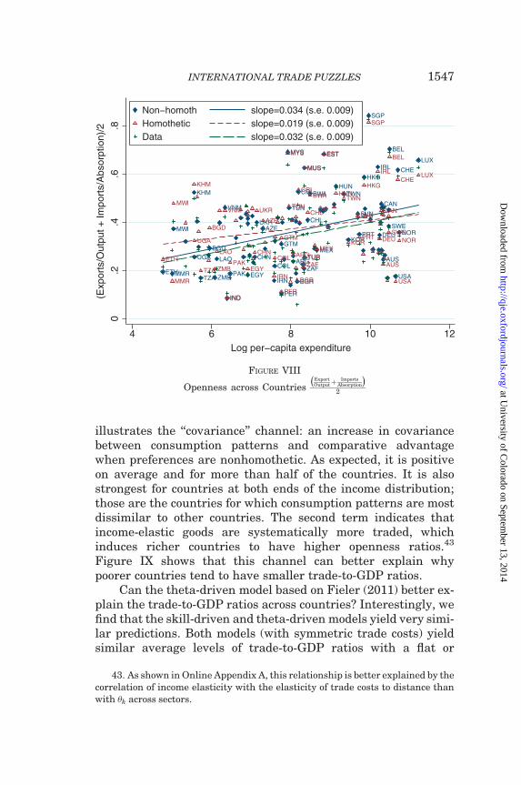
illustrates the ‘‘covariance’’ channel: an increase in covariancebetween consumption patterns and comparative advantagewhen preferences are nonhomothetic. As expected, it is positiveon average and for more than half of the countries. It is alsostrongest for countries at both ends of the income distribution;those are the countries for which consumption patterns are mostdissimilar to other countries. The second term indicates thatincome-elastic goods are systematically more traded, whichinduces richer countries to have higher openness ratios.43

Figure IX shows that this channel can better explain whypoorer countries tend to have smaller trade-to-GDP ratios.

Can the theta-driven model based on Fieler (2011) better ex-plain the trade-to-GDP ratios across countries? Interestingly, wefind that the skill-driven and theta-driven models yield very simi-lar predictions. Both models (with symmetric trade costs) yieldsimilar average levels of trade-to-GDP ratios with a flat or

ARG AUS

AZE

BEL

BGD

BGR

BWA

CAN

CHE

CHL

CHNCOL

CRI

DEU

EGY

EST

ETH

GTM

HKG

HUN

IND

IRL

IRN

KHM

KOR

LAO

LUX

MEX

MLT

MMR

MUS

MWI

MYS

NOR

PAK

PER

PRT

SGP

SVN

SWE

TUN

TUR

TWN

TZA

UGA

UKR

USA

VNM

ZAFZMB

ARG

AUS

AZE

BEL

BGD

BGR

BWA

CAN

CHE

CHL

CHNCOL

CRI

DEU

EGY

EST

ETH

GTM

HKGHUN

IND

IRL

IRN

KHM

KOR

LAO

LUX

MEX

MLT

MMR

MUS

MWI

MYS

NOR

PAK

PER

PRT

SGP

SVN

SWE

TUN

TUR

TWN

TZA

UGA

UKR

USA

VNM

ZAFZMB

0.2

.4.6

.8(E

xpor

ts/O

utpu

t + Im

port

s/A

bsor

ptio

n)/2

4 6 8 10 12Log per−capita expenditure

Non−homoth slope=0.034 (s.e. 0.009)Homothetic slope=0.019 (s.e. 0.009)Data slope=0.032 (s.e. 0.009)

FIGURE VIII

Openness across CountriesExportOutputþ

ImportsAbsorption

� 2

43. As shown in Online Appendix A, this relationship is better explained by thecorrelation of income elasticity with the elasticity of trade costs to distance thanwith �k across sectors.


at University of C



ownloaded from



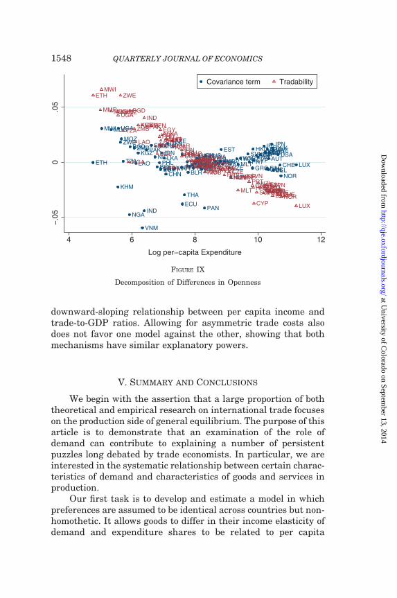
downward-sloping relationship between per capita income andtrade-to-GDP ratios. Allowing for asymmetric trade costs alsodoes not favor one model against the other, showing that bothmechanisms have similar explanatory powers.

V. Summary and Conclusions

We begin with the assertion that a large proportion of boththeoretical and empirical research on international trade focuseson the production side of general equilibrium. The purpose of thisarticle is to demonstrate that an examination of the role ofdemand can contribute to explaining a number of persistentpuzzles long debated by trade economists. In particular, we areinterested in the systematic relationship between certain charac-teristics of demand and characteristics of goods and services inproduction.

Our first task is to develop and estimate a model in whichpreferences are assumed to be identical across countries but non-homothetic. It allows goods to differ in their income elasticity ofdemand and expenditure shares to be related to per capita

ALBARG

ARM

AUS

AUT

AZE

BEL

BGD

BGRBLR

BOLBRA

BWA

CANCHECHL

CHN

COL

CRICYP

CZE

DEUDNK

ECU

EGY

ESPEST

ETHFIN

FRAGBR

GEO GRCGTM

HKG

HRV

HUN

IDN

IND

IRL

IRN

ITAJPN

KAZ

KGZ

KHM

KORLAO

LKALTU LUXLVA

MAR

MDG

MEX MLT

MOZ

MUS

MWI

MYS

NGA

NICNLD

NOR

NZLPAK

PAN

PERPHL POL PRTPRY

ROURUS

SEN

SGP

SVK

SVNSWE

THA

TUNTUR

TWNTZA

UGA

UKR

URY

USAVEN

VNM

ZAF

ZMBZWE

ALBARG

ARM

AUSAUT

AZE

BEL

BGD

BGRBLRBOL

BRA

BWA

CANCHE

CHL

CHN

COL

CRI

CYP

CZE

DEUDNK

ECU

EGY

ESP

EST

ETH

FINFRAGBR

GEO

GRC

GTM

HKG

HRVHUN

IDN

IND

IRL

IRN

ITAJPN

KAZ

KGZ

KHM

KOR

LAOLKA

LTU

LUX

LVA

MAR

MDG

MEX

MLT

MMR MOZ

MUS

MWI

MYSNGA

NIC

NLDNOR

NZL

PAK

PANPER

PHL

POL

PRT

PRY

ROURUS

SEN

SGP

SVKSVN

SWE

THA

TUNTUR

TWN

TZA

UGA

UKR

URY

USA

VEN

VNM

ZAF

ZMB

ZWE

−.0

50

.05

4 6 8 10 12

Log per−capita Expenditure

Covariance term Tradability

FIGURE IX

Decomposition of Differences in Openness


at University of C



ownloaded from


income. Both economically and statistically, we find large devi-ations of income elasticity estimates from the unitary valuesimplied by homothetic preferences. The next step is to relatethese income elasticities of demand to factor intensities of goodsin production. Here we find a strong, positive correlation (higherthan 45%) between a good’s income elasticity of demand and itsskilled-labor intensity in production. The correlation is robust tothe inclusion of trade costs and a number of other factors.

We then investigate the implications of nonhomothetic pref-erences and their relationship to factor intensities. Our first re-sults assess their contribution to the missing trade puzzle. Wefind that they can reduce the overpredicted variance in the factorcontent of trade by more than half. This result is driven by asupply-demand correlation that is absent under homothetic pref-erences: countries tend to specialize in the consumption of thesame goods that they are specialized in producing.

Another set of results relate to trade patterns and the selec-tion of trading partners. Our findings imply that high-incomecountries have a comparative advantage in high-income-elasti-city goods and services, because these are skilled-labor intensiveand because the high-income countries are skilled-labor abun-dant. This suggests that countries should be more likely totrade with countries of similar income level and we verify thatthis is the case. Although this mechanism also predicts lowerlevels of trade-to-GDP ratios, we find its explanatory power tobe smaller than another channel through which nonhomotheti-city affects openness to trade: the fact that income-elastic goodsare systematically more tradable. Results show that the twochannels together are capable of closely replicating the positiverelationship between per capita income and openness found inthe data.

While the correlation between skill intensity and incomeelasticity affects trade patterns and trade volumes, we wouldlike to point out that it may also have important implicationsfor the skill premium (skilled worker wages relative to unskilledworker wages). In particular, it can generate a positive effect ofTFP growth on this premium. The intuition is simple. As prod-uctivity increases, people become richer and consume more goodsfrom income-elastic industries, which are, as we show, more in-tensive in skilled labor. This increases the demand for skilledlabor relative to unskilled labor and thus increases the relativewage of skilled workers. In the working paper version of this


at University of C



ownloaded from


article (Caron, Fally, and Markusen 2012), we used our modeland estimated parameters to simulate productivity (TFP)growth and found a large effect on the skill premium, which ledus to believe that the demand side could potentially play an im-portant role.44

Finally, nonhomothetic preferences may also influence thedirection of technological change. If income-elastic goods tend tobe consumed and produced in countries that are abundant inskilled labor, the production of these goods should be associatedwith a larger demand for technologies compatible with skilledlabor. This mechanism could partially explain the positive correl-ation between skill intensity and income elasticity documented inthis article.

Massachusetts Institute of Technology, Joint Program

on the Science and Policy of Global Change and ETH

Zurich

University of California, Berkeley, and University of

Colorado, Boulder

University of Colorado, Boulder

Supplementary Material

An Online Appendix for this article can be found at QJEonline (qje.oxfordjournals.org).

References

Anderson, James E., and Eric van Wincoop, ‘‘Gravity with Gravitas: A Solution tothe Border Puzzle,’’ American Economic Review, 93 (2003), 170–192.

Athey, Susan, ‘‘Monotone Comparative Statics under Uncertainty,’’ QuarterlyJournal of Economics, 117 (2002), 187–223.

Barro, Robert and Jong-Wha Lee, ‘‘A New Data Set of Educational Attainment inthe World, 1950–2010,’’ forthcoming, Journal of Development Economics.

Bergstrand, Jeffrey, ‘‘The Heckscher-Ohlin-Samuelson Model, the LinderHypothesis and the Determinants of Bilateral Intra-industry Trade,’’Economic Journal, 100, no. 403 (1990), 1216–1229.

Bernasconi, Claudia, ‘‘Income Similarity and Bilateral Trade Flows,’’ Universityof Zurich working paper (2011).

Caliendo, Lorenzo, and Fernando Parro, ‘‘Estimates of the Trade and WelfareEffects of NAFTA,’’ NBER Working Paper No. 18508 (2012).

Caron, Justin, Thibault Fally, and James R. Markusen, ‘‘Skill Premium andTrade Puzzles: A Solution Linking Production and Preferences,’’ NBERWorking Paper No. 18131 (2012).

44. The argument is not limited to the reallocation of consumption across indus-tries: within-industry heterogeneity in product quality and income elasticity canplay a similar role if the production of higher-quality products is more intensive inskilled labor.


at University of C



ownloaded from



Cassing, James, and Shuichiro Nishioka, ‘‘Nonhomothetic Tastes and MissingTrade in Factor Services,’’ Working paper (2009).

Chaney, Thomas, ‘‘Distorted Gravity: The Intensive and Extensive Margins ofInternational Trade,’’ American Economic Review, 98 (2008), 1707–1721.

Chao, Hung-po, Sehun Kim, and Alan S. Manne, ‘‘Computation of Equilibria forNonlinear Economies: Two Experimental Model,’’ Journal of PolicyModeling, 4 (1982), 23–43.

Costinot, Arnaud, ‘‘An Elementary Theory of Comparative Advantage,’’Econometrica, 77 (2009), 1165–1192.

Costinot, Arnaud, Dave Donaldson, and Ivana Komunjer, ‘‘What Goods DoCountries Trade? A Quantitative Exploration of Ricardo’s Ideas,’’ Review ofEconomics Studies, 79 (2012), 581–608.

Davis, Donald R., and David E. Weinstein, ‘‘An Account of Global Factor Trade,’’American Economic Review, 91 (2001), 1423–1453.

de Sousa, Jose, ‘‘The Currency Union Effect on Trade Is Decreasing over Time,’’Economics Letters, 117 (2012), 917–920.

Deaton, Angus, and John Muellbauer, Economics and Consumer Behavior(Cambridge: Cambridge University Press, 1980).

Donaldson, Dave, ‘‘Railroads of the Raj: Estimating the Impact of TransportationInfrastructure,’’ The American Economic Review (forthcoming).

Eaton, Jonathan, and Samuel Kortum, ‘‘Technology, Geography, and Trade,’’Econometrica, 79 (2002), 1453–1498.

Eaton, Jonathan, Samuel Kortum, and Francis Kramarz, ‘‘An Anatomy ofInternational Trade: Evidence from French Firms,’’ Econometrica, 79(2011), 1453–1498.

Fajgelbaum, Pablo, Gene M. Grossman, and Elhanan Helpman, ‘‘IncomeDistribution, Product Quality, and International Trade,’’ Journal ofPolitical Economy, 119 (2011), 721–765.

Fally, Thibault, ‘‘Structural Gravity and Fixed Effects,’’ Mimeo, University ofColorado (2012).

Fally, Thibault, Rodrigo Paillacar, and Cristina Terra, ‘‘Economic Geography andWages in Brazil: Evidence from Micro-data,’’ Journal of DevelopmentEconomics, 91 (2010), 155–168.

Fieler, Ana Cecilia, ‘‘Non-Homotheticity and Bilateral Trade: Evidence and aQuantitative Explanation,’’ Econometrica, 79 (2011), 1069–1101.

Hallak, Juan Carlos, ‘‘Product Quality and the Direction of Trade,’’ Journal ofInternational Economics, 68 (2006), 238–265.

———, ‘‘A Product-Quality View of the Linder Hypothesis,’’ Review of Economicsand Statistics, 92, no. 3 (2010), 453–466.

Hallak, Juan Carlos, and Peter K. Schott, ‘‘Estimating Cross-CountryDifferences in Product Quality,’’ Quarterly Journal of Economics, 126(2011), 417–474.

Hanoch, Giora, ‘‘Production and Demand Models with Direct or Indirect ImplicitAdditivity,’’ Econometrica, 43 (1975), 395–419.

Head, Keith, and Thierry Mayer, ‘‘Regional Wage and Employment Responses toMarket Potential in the EU,’’ Regional Science and Urban Economics, 36, no.5 (2006), 573–594.

Hunter, Linda, ‘‘The Contribution of Non-homothetic Preferences to Trade,’’Journal of International Economics, 30 (1991), 345–358.

Hunter, Linda, and James R. Markusen, Per-Capita Income as a Determinant ofTrade (Cambridge, MA: MIT Press, 1988).

Khandelwal, Amit, ‘‘The Long and Short (of) Quality Ladders,’’ Review ofEconomic Studies, 77 (2010), 1450–1476.

Lewis, Jeffrey B., and Drew A. Linzer, ‘‘Estimating Regression Models in whichthe Dependent Variable Is Based on Estimates,’’ Political Analysis, 13, no. 4(2005), 345–364.

Linder, Staffan B. An Essay on Trade and Transformation (Stockholm: Almqvistand Wiksell, 1961).

Markusen, James R., ‘‘Explaining the Volume of Trade: An Eclectic Approach,’’American Economic Review, 76 (1986), 1002–1011.

———, ‘‘Putting Per-Capita Income Back into Trade Theory,’’ Journal ofInternational Economics, 90 (2013), 255–265.


at University of C



ownloaded from


Martinez-Zarzoso, Inmaculada, and Sebastian Vollmer, ‘‘Bilateral Trade Flowsand Income-Distribution Similarity,’’ BE Working Papers on InternationalEconomics and Finance (2011).

Matsuyama, Kiminori, ‘‘A Ricardian Model with a Continuum of Goods underNon-Homothetic Preferences: Demand Complementarities, IncomeDistribution, and North-South Trade,’’ Journal of Political Economy, 108(2000), 1093–2000.

Mayer, Thierry, and Soledad Zignago, ‘‘Notes on CEPII’s Distances Measures: TheGeoDist Database,’’ Working Paper 2011-25, CEPII Research Center (2011).

McCallum, John, ‘‘National Borders Matter: Canada-U.S. Regional TradePatterns,’’ American Economic Review, American Economic Association, 85(1995), 615–623.

Narayanan, Badri G., and Terrie L. Walmsley, ‘‘Global Trade, Assistance, andProduction: The GTAP 7 Data Base,’’ Center for Global Trade Analysis,Purdue University (2008).

Pagan, Adrian, ‘‘Econometric Issues in the Analysis of Regressions withGenerated Regressors,’’ International Economic Review, 25 (1984), 221–247.

Redding, Stefan James, and Anthony J. Venables, ‘‘Economic Geography andInternational Inequality,’’ Journal of International Economics, 62 (2004),53–82.

Reimer, Jeffery J., and Thomas W. Hertel, ‘‘Nonhomothetic Preferences andInternational Trade,’’ Review of International Economics, 18 (2010), 408–425.

Santos Silva, J. M. C. and Silvana Tenreyro, ‘‘The Log of Gravity,’’ The Review ofEconomics and Statistics, MIT Press, 88 (2006), 641–658.

Simonovska, Ina, ‘‘Income Differences and Prices of Tradeables,’’ NBER WorkingPaper No. 16233 (2010).

Simonovska, Ina, and Michael Waugh, ‘‘The Elasticity of Trade: Estimates andEvidence,’’ UC Davis Working Paper No. 11-2 (2010).

Trefler, Daniel, ‘‘The Case of Missing Trade and Other Mysteries,’’ AmericanEconomic Review, 85 (1995), 1029–1046.

Trefler, Daniel, and Susan Zhu, ‘‘The Structure of Factor Content Predictions,’’Journal of International Economics, 82 (2010), 195–207.

Verhoogen, Eric A., ‘‘Trade, Quality Upgrading, and Wage Inequality in theMexican Manufacturing Sector,’’ Quarterly Journal of Economics, 123(2008), 489–530.

Waugh, Michael, ‘‘International Trade and Income Differences,’’ AmericanEconomic Review, 100 (2010), 2093–2124.

Yi, Kei-Mu, ‘‘Can Multistage Production Explain the Home Bias in Trade?,’’American Economic Review, American Economic Association, 100 (2010),364–393.


at University of C



ownloaded from


international trade puzzles: a solution...

Documents