slepc current achievements and plans for the futureslepc.upv.es/material/slides/slepc-anl-1p.pdf ·...

Linear Eigenvalue ProblemsNon-Linear Eigenvalue Problems

Additional Features

SLEPcCurrent Achievements and Plans for the Future

Jose E. Roman

D. Sistemes Informatics i ComputacioUniversitat Politecnica de Valencia, Spain

Celebrating 20 years of PETSc, Argonne – June, 2015

1/36


Additional Features

SLEPc: Scalable Library for Eigenvalue Problem Computations

A general library for solving large-scale sparse eigenproblems onparallel computers

I Linear eigenproblems (standard or generalized, real orcomplex, Hermitian or non-Hermitian)

I Also support for SVD, PEP, NEP and more

Ax = λx Ax = λBx Avi = σiui T (λ)x = 0

Authors: J. E. Roman, C. Campos, E. Romero, A. Tomas

http://slepc.upv.es

Current version: 3.6 (released June 2015)

2/36

http://slepc.upv.es


Additional Features

Timeline

Jose

Andres

Eloy

Carmen

Alejandro

Krylov-Schur

Jacobi-Davidson

Polynomial solvers

First release slepc-3.0

2000 2005 2010 2015

Jose Roman Andres Tomas Eloy Romero CarmenCampos

AlejandroLamas

3/36


Additional Features

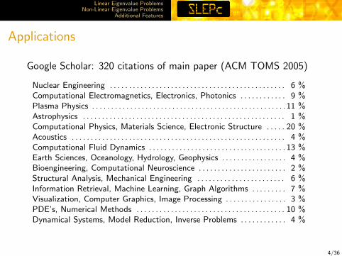
Applications

Google Scholar: 320 citations of main paper (ACM TOMS 2005)

Nuclear Engineering . . . . . . . . . . . . . . . . . . . . . . . . . . . . . . . . . . . . . . . . . . . . . . 6 %Computational Electromagnetics, Electronics, Photonics . . . . . . . . . . . . 9 %Plasma Physics . . . . . . . . . . . . . . . . . . . . . . . . . . . . . . . . . . . . . . . . . . . . . . . . . . .11 %Astrophysics . . . . . . . . . . . . . . . . . . . . . . . . . . . . . . . . . . . . . . . . . . . . . . . . . . . . . 1 %Computational Physics, Materials Science, Electronic Structure . . . . . 20 %Acoustics . . . . . . . . . . . . . . . . . . . . . . . . . . . . . . . . . . . . . . . . . . . . . . . . . . . . . . . . 4 %Computational Fluid Dynamics . . . . . . . . . . . . . . . . . . . . . . . . . . . . . . . . . . . . 13 %Earth Sciences, Oceanology, Hydrology, Geophysics . . . . . . . . . . . . . . . . . 4 %Bioengineering, Computational Neuroscience . . . . . . . . . . . . . . . . . . . . . . . 2 %Structural Analysis, Mechanical Engineering . . . . . . . . . . . . . . . . . . . . . . . 6 %Information Retrieval, Machine Learning, Graph Algorithms . . . . . . . . . 7 %Visualization, Computer Graphics, Image Processing . . . . . . . . . . . . . . . . 3 %PDE’s, Numerical Methods . . . . . . . . . . . . . . . . . . . . . . . . . . . . . . . . . . . . . . . 10 %Dynamical Systems, Model Reduction, Inverse Problems . . . . . . . . . . . . 4 %

4/36


Additional Features

Problem Classes

The user must choose the most appropriate solver for eachproblem class

Problem class Model equation ModuleLinear eigenproblem Ax = λx, Ax = λBx EPS

Quadratic eigenproblem (K + λC + λ2M)x = 0 †Polynomial eigenproblem (A0 + λA1 + · · ·+ λdAd)x = 0 PEP

Nonlinear eigenproblem T (λ)x = 0 NEP

Singular value decomp. Av = σu SVD

Matrix function y = f(A)v MFN† QEP removed in version 3.5

Auxiliary classes: ST, BV DS, RG, FN

5/36


Additional Features

PETSc

Vectors

Standard CUSP

Index Sets

Indices Block Stride Other

Matrices

CompressedSparse Row

BlockCSR

SymmetricBlock CSR

Dense CUSP Other

Preconditioners

AdditiveSchwarz

BlockJacobi

Jacobi ILU ICC LU Other

Krylov Subspace Methods

GMRES CG CGS Bi-CGStab TFQMR Richardson Chebychev Other

Nonlinear Systems

LineSearch

TrustRegion Other

Time Steppers

EulerBackward

Euler

PseudoTime Step Other

SLEPc

Polynomial Eigensolver

TOARQ-

ArnoldiLinear-ization

Nonlinear Eigensolver

SLP RIIN-

ArnoldiInterp.

SVD Solver

CrossProduct

CyclicMatrix

LanczosThick R.Lanczos

M. Function

Krylov

Linear Eigensolver

Krylov-Schur GD JD LOBPCG CISS Other

Spectral Transformation

Shift Shift-and-invert Cayley Preconditioner

BV DS RG FN

6/36


Additional Features

Outline

1 Linear Eigenvalue ProblemsEPS: Eigenvalue Problem SolverSelection of wanted eigenvaluesPreconditioned eigensolvers

2 Non-Linear Eigenvalue ProblemsPEP: Polynomial EigensolversNEP: General Nonlinear Eigensolvers

3 Additional FeaturesMFN: Matrix FunctionAuxiliary Classes

7/36


Additional Features

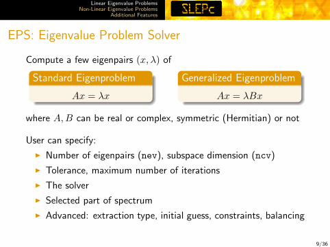
EPS: Eigenvalue Problem Solver

Compute a few eigenpairs (x, λ) of

Standard Eigenproblem

Ax = λx

Generalized Eigenproblem

Ax = λBx

where A,B can be real or complex, symmetric (Hermitian) or not

User can specify:

I Number of eigenpairs (nev), subspace dimension (ncv)

I Tolerance, maximum number of iterations

I The solver

I Selected part of spectrum

I Advanced: extraction type, initial guess, constraints, balancing

9/36


Additional Features

Available Eigensolvers

User code is independent of the selected solver

1. Basic methodsI Single vector iteration: power iteration, inverse iteration, RQII Subspace iteration with Rayleigh-Ritz projection and lockingI Explicitly restarted Arnoldi and Lanczos

2. Krylov-Schur, including thick-restart Lanczos3. Generalized Davidson, Jacobi-Davidson4. Conjugate gradient methods: LOBPCG, RQCG5. CISS, a contour-integral solver6. External packages, and LAPACK for testing

. . . but some solvers are specific for a particular case:

I LOBPCG computes smallest λi of symmetric problemsI CISS allows computation of all λi within a region

10/36


Additional Features

Selection of Eigenvalues (1): Basic

Largest/smallest magnitude, or real (or imaginary) part

Example: QC2534

-eps nev 6

-eps ncv 128

-eps largest imaginary

Computedeigenvalues

11/36


Additional Features

Selection of Eigenvalues (2): Region Filtering

RG: Region

I A region of the complex plane (interval, polygon, ellipse, ring)

I Used as an inclusion (or exclusion) region

Example: sign1 (NLEVP) n = 225, allλ lie at unit circle, accumulate at ±1

-eps nev 6

-rg type interval

-rg interval endpoints -0.7,0.7,-1,1

12/36


Additional Features

Selection of Eigenvalues (3): Closest to Target

Shift-and-invert is used to compute interior eigenvalues

Ax = λBx =⇒ (A− σB)−1Bx = θx

I Trivial mapping of eigenvalues: θ = (λ− σ)−1

I Eigenvectors are not modified

I Very fast convergence close to σ

Things to consider:

I Implicit inverse (A− σB)−1 via linear solves

I Direct linear solver for robustness

I Less effective for eigenvalues far away from σ

13/36


Additional Features

Selection of Eigenvalues (4): Interval (in GHEP)Indefinite (block-)triangular factorization: A− σB = LDLT

A byproduct is the number of eigenvalues on the left of σ (inertia)

ν(A− σB) = ν(D)

Spectrum Slicing strategy:

I Multi-shift scheme that sweeps all the interval

I Compute eigenvalues by chunks

I Use inertia to validate sub-intervals

a b

σ1 σ2 σ3

C. Campos and J. E. Roman, “Strategies for spectrum slicing based on restarted Lanczosmethods”, Numer. Algorithms, 60(2):279–295, 2012.

new Multi-communicator version, one subinterval per partition14/36


Additional Features

Selection of Eigenvalues (5): All inside a Region

CISS solver1: compute all eigenvalues inside a given region

Example: QC2534

-eps type ciss

-rg type ellipse

-rg ellipse center -.8-.1i

-rg ellipse radius 0.2

-rg ellipse vscale 0.1

1Contributed by Y. Maeda, T. Sakurai15/36


Additional Features

Selection of Eigenvalues (5): All inside a Region

Example: MHD1280 with CISS

I Alfven spectra: eigenvalues inintersection of the branches

0-100-200

0

500

-500

RG=ellipse, center=0, radius=1

0-1 1

0

1

-1

RG=ring, center=0, radius=0.5,width=0.2, angle=0.25..0.5

0-0.5-10

0.5

1

16/36


Additional Features

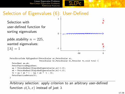
Selection of Eigenvalues (6): User-Defined

Selection withuser-defined function forsorting eigenvalues

pdde stability n = 225,wanted eigenvalues:‖λ‖ = 1

0

1

-1

0-50

PetscErrorCode MyEigenSort(PetscScalar ar,PetscScalar ai,

PetscScalar br,PetscScalar bi,PetscInt *r,void *ctx)

PetscReal aa,ab;

PetscFunctionBeginUser;

aa = PetscAbsReal(SlepcAbsEigenvalue(ar,ai)-1.0);

ab = PetscAbsReal(SlepcAbsEigenvalue(br,bi)-1.0);

*r = aa > ab ? 1 : (aa < ab ? -1 : 0);

PetscFunctionReturn(0);

Arbitrary selection: apply criterion to an arbitrary user-definedfunction φ(λ, x) instead of just λ

17/36


Additional Features

Preconditioned Eigensolvers

Pitfalls of shift-and-invert:

I Direct solvers have high cost, limited scalability

I Inexact shift-and-invert (i.e., with iterative solver) not robust

Preconditioned eigensolvers try to overcome these problems

1. Davidson-type solvers

I Jacobi-Davidson: correction equation with iterative solver

I Generalized Davidson: simple preconditioner application

E. Romero and J. E. Roman, “A parallel implementation of Davidson methods for large-scale eigenvalue problems in SLEPc”, ACM Trans. Math. Softw., 40(2):13, 2014.

2. Conjugate Gradient-type solvers (for GHEP)

I RQCG: CG for the minimization of the Rayleigh Quotient

I new LOBPCG: Locally Optimal Block Preconditioned CG

18/36


Additional Features

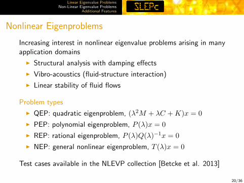
Nonlinear Eigenproblems

Increasing interest in nonlinear eigenvalue problems arising in manyapplication domains

I Structural analysis with damping effects

I Vibro-acoustics (fluid-structure interaction)

I Linear stability of fluid flows

Problem types

I QEP: quadratic eigenproblem, (λ2M + λC +K)x = 0

I PEP: polynomial eigenproblem, P (λ)x = 0

I REP: rational eigenproblem, P (λ)Q(λ)−1x = 0

I NEP: general nonlinear eigenproblem, T (λ)x = 0

Test cases available in the NLEVP collection [Betcke et al. 2013]

20/36


Additional Features

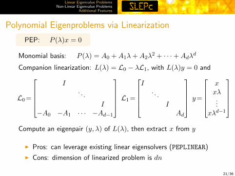
Polynomial Eigenproblems via Linearization

PEP: P (λ)x = 0

Monomial basis: P (λ) = A0 +A1λ+A2λ2 + · · ·+Adλ

d

Companion linearization: L(λ) = L0 − λL1, with L(λ)y = 0 and

L0=

I

. . .

I−A0 −A1 · · · −Ad−1

L1=

I

. . .

IAd

y=

xxλ...

xλd−1

Compute an eigenpair (y, λ) of L(λ), then extract x from y

I Pros: can leverage existing linear eigensolvers (PEPLINEAR)

I Cons: dimension of linearized problem is dn

21/36


Additional Features

PEP: Krylov Methods with Compact Representation

Arnoldi relation: SVj =[Vj v

]Hj , S := L−11 L0

Write Arnoldi vectors as v = vec[v0, . . . , vd−1

]Block structure of S allows an implicit representation of the basis

I Q-Arnoldi: V i+1j =

[V ij vi

]Hj

I TOAR:[V ij vi

]= Uj+d

[Gij gi

]Arnoldi relation in the compact representation:

S(Id ⊗ Uj+d−1)Gj = (Id ⊗ Uj+d)[Gj g

]Hj

PEPTOAR is the default solver

I Memory-efficient (also in terms of computational cost)

I Many features: restart, locking, scaling, extraction, refinement

C. Campos and J. E. Roman, “Parallel Krylov solvers for the polynomial eigenvalue problemin SLEPc”, submitted, 2015.

22/36


Additional Features

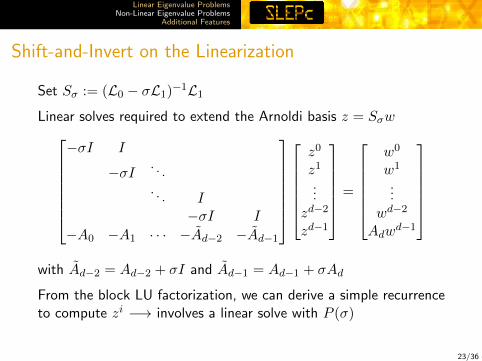
Shift-and-Invert on the Linearization

Set Sσ := (L0 − σL1)−1L1Linear solves required to extend the Arnoldi basis z = Sσw−σI I

−σI . . .. . . I

−σI I

−A0 −A1 · · · −Ad−2 −Ad−1

z0

z1

...zd−2

zd−1

=

w0

w1

...wd−2

Adwd−1

with Ad−2 = Ad−2 + σI and Ad−1 = Ad−1 + σAd

From the block LU factorization, we can derive a simple recurrenceto compute zi −→ involves a linear solve with P (σ)

23/36


Additional Features

Quantum Dot Simulation

3D pyramidal quantum dot discretized with finite volumes

Tsung-Min Hwang et al. (2004). “Numerical Simulationof Three Dimensional Pyramid Quantum Dot,” Journal ofComputational Physics, 196(1): 208-232.

Quintic polynomial, n ≈ 12 mill.

Scaling for tol=10−8, nev=5, ncv=40 with

inexact shift-and-invert (bcgs+bjacobi) 2 4 8 16 32 64 128

103

104

Tim

e[s

]

TOARPlain

24/36


Additional Features

PEP: Additional Features

Non-Monomial polynomial basis

P (λ) = A0φ0(λ) +A1φ1(λ) + · · ·+Adφd(λ)

I Implemented for Chebyshev, Legendre, Laguerre, Hermite

I Enables polynomials of arbitrary degree

Newton iterative refinement

I Optional for ill-conditioned problems

I Implemented for single eigenpairs as well as invariant pairs

Other solvers not based on linearization

new PEPJD provides Jacobi-Davidson for polynomial eigenproblems

25/36


Additional Features

General Nonlinear Eigenproblems

NEP: T (λ)x = 0, x 6= 0

T : Ω→ Cn×n is a matrix-valued function analytic on Ω ⊂ C

Example 1: Rational eigenproblem arising in the study of freevibration of plates with elastically attached masses

−Kx+ λMx+

k∑j=1

λ

σj − λCjx = 0

All matrices symmetric, K > 0,M > 0 and Cj have small rank

Example 2: Discretization of parabolic PDE with time delay τ

(−λI +A+ e−τλB)x = 0

26/36


Additional Features

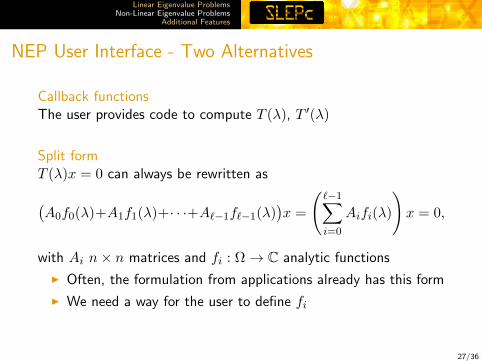
NEP User Interface - Two Alternatives

Callback functionsThe user provides code to compute T (λ), T ′(λ)

Split formT (λ)x = 0 can always be rewritten as

(A0f0(λ)+A1f1(λ)+· · ·+A`−1f`−1(λ)

)x =

(`−1∑i=0

Aifi(λ)

)x = 0,

with Ai n× n matrices and fi : Ω→ C analytic functions

I Often, the formulation from applications already has this form

I We need a way for the user to define fi

27/36


Additional Features

FN: Mathematical Functions

The FN class provides a few predefined functions

I The user specifies the type and relevant coefficients

I Also supports evaluation of fi(X) on a small matrix

Basic functions:

1. Rational function (includes polynomial)

r(x) =p(x)

q(x)=

α1xn−1 + · · ·+ αn−1x+ αn

β1xm−1 + · · ·+ βm−1x+ βm

2. Other: exp, log, sqrt, ϕ-functions

new and a way to combine functions (with addition, multiplication,division or function composition), e.g.:

f(x) = (1− x2) exp

(−x

1 + x2

)28/36


Additional Features

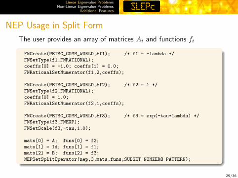
NEP Usage in Split Form

The user provides an array of matrices Ai and functions fi

FNCreate(PETSC_COMM_WORLD,&f1); /* f1 = -lambda */

FNSetType(f1,FNRATIONAL);

coeffs[0] = -1.0; coeffs[1] = 0.0;

FNRationalSetNumerator(f1,2,coeffs);

FNCreate(PETSC_COMM_WORLD,&f2); /* f2 = 1 */

FNSetType(f2,FNRATIONAL);

coeffs[0] = 1.0;

FNRationalSetNumerator(f2,1,coeffs);

FNCreate(PETSC_COMM_WORLD,&f3); /* f3 = exp(-tau*lambda) */

FNSetType(f3,FNEXP);

FNSetScale(f3,-tau,1.0);

mats[0] = A; funs[0] = f2;

mats[1] = Id; funs[1] = f1;

mats[2] = B; funs[2] = f3;

NEPSetSplitOperator(nep,3,mats,funs,SUBSET_NONZERO_PATTERN);

29/36


Additional Features

Currently Available NEP Solvers

1. Single-vector iterations

I Residual inverse iteration (RII) [Neumaier 1985]

I Successive linear problems (SLP) [Ruhe 1973]

2. Nonlinear Arnoldi [Voss 2004]

I Performs a projection on RII iterates, V ∗j T (λ)Vjy = 0

I Requires the split form

3. Polynomial Interpolation: use PEP to solve P (λ)x = 0

I P (·) is the interpolation polynomial in Chebyshev basis

4. new Contour Integral

I Extension of the CISS method in EPS

30/36


Additional Features

MFN: Matrix Function

From the Taylor series expansion of eA

y = eAv = v +A

1!v +

A2

2!v + · · ·

so y can be approximated by an element of Km(A, v)

Given an Arnoldi decomposition AVm = Vm+1Hm

y = βVm+1 exp(Hm)e1

This extends to other functions y = f(A)v

What is needed:

I Efficient construction of the Krylov subspace

I Computation of f(X) for a small dense matrix → FN

32/36


Additional Features

Auxiliary Classes

I ST: Spectral TransformationI FN: Mathematical Function

I Represent the constituent functions of the nonlinear operatorin split form

I Function to be used when computing f(A)v

I RG: Region (of the complex plane)I Discard eigenvalues outside the wanted regionI Compute all eigenvalues inside a given region

I DS: Direct Solver (or Dense System)I High-level wrapper to LAPACK functions

I BV: Basis Vectors

33/36


Additional Features

BV: Basis VectorsBV provides the concept of a block of vectors that represent thebasis of a subspace; sample operations:

BVMult Y = βY + αXQBVAXPY Y = Y + αXBVDot M = Y ∗XBVMatProject M = Y ∗AXBVScale Y = αY

Goal: to increase arithmetic intensity (BLAS-2 vs BLAS-1)

$ ./ex9 -n 8000 -eps_nev 32 -log_summary -bv_type vecs

BVMult 32563 1.0 3.2903e+01 1.0 6.61e+10 1.0 0.0e+00 0.0e+00 ... 2009

BVDot 32064 1.0 1.6213e+01 1.0 5.07e+10 1.0 0.0e+00 0.0e+00 ... 3128

$ ./ex9 -n 8000 -eps_nev 32 -log_summary -bv_type mat

BVMult 32563 1.0 2.4755e+01 1.0 8.24e+10 1.0 0.0e+00 0.0e+00 ... 3329

BVDot 32064 1.0 1.4507e+01 1.0 5.07e+10 1.0 0.0e+00 0.0e+00 ... 3497

Even better in block solvers (LOBPCG): BLAS-3, MatMatMult

34/36


Additional Features

Plans for Future Developments

Short term plans:

I More EPS solvers: improved LOBPCG, block Krylov methods

I More PEP solvers: SOAR, improved JD

I More NEP solvers: NLEIGS

I More MFN solvers: rational Krylov

I Improved GPU support in BV

A new solver class for Matrix equations

I Krylov methods for the continuous-time Lyapunov equation

AX +XAT = C

I Other equations: Sylvester, Stein, Ricatti

35/36


Additional Features

Acknowledgements

Thanks to:

I The PETSc team

I Contributors

I Users providing feedback

Funding agencies:

Computing resources:

36/36

slepc current achievements and plans for the futureslepc.upv.es/material/slides/slepc-anl-1p.pdf ·...

Documents