s.k.p institute of technology tiruvannamalai 606 611
TRANSCRIPT

S.K.P INSTITUTE OF TECHNOLOGY Tiruvannamalai– 606 611
Verified by : HOD Prepared by: N.Gopinath
Approved by:PRINCIPAL
CS2060 HIGH SPEED NETWORKS
COURSE NOTES FOR ALL THE 5 UNITS

S.K.P INSTITUTE OF TECHNOLOGY Tiruvannamalai– 606 611
Verified by : HOD Prepared by: N.Gopinath
Approved by:PRINCIPAL
Unit I
Frame relay Networks
Frame Relay often is described as a streamlined version of X.25, offering fewer of the robust capabilities,
such as windowing and retransmission of last data that are offered in X.25.
Frame Relay Devices
Devices attached to a Frame Relay WAN fall into the following two general categories:
• Data terminal equipment (DTE) • Data circuit-terminating equipment (DCE)
DTEs generally are considered to be terminating equipment for a specific network and typically are located
on the premises of a customer. In fact, they may be owned by the customer. Examples of DTE devices are
terminals, personal computers, routers, and bridges.
DCEs are carrier-owned internetworking devices. The purpose of DCE equipment is to provide clocking
and switching services in a network, which are the devices that actually transmit data through the WAN. In
most cases, these are packet switches. Figure 10-1 shows the relationship between the two categories of
devices.
Standard Frame Relay Frame
Standard Frame Relay frames consist of the fields illustrated in Figure 10-4.
Figure Five Fields Comprise the Frame Relay Frame
Each frame relay PDU consists of the following fields:
1. Flag Field. The flag is used to perform high level data link synchronization which indicates the
beginning and end of the frame with the unique pattern 01111110. To ensure that the 01111110
pattern does not appear somewhere inside the frame, bit stuffing and destuffing procedures are
used.

S.K.P INSTITUTE OF TECHNOLOGY Tiruvannamalai– 606 611
Verified by : HOD Prepared by: N.Gopinath
Approved by:PRINCIPAL
2. Address Field. Each address field may occupy either octet 2 to 3, octet 2 to 4, or octet 2 to 5,
depending on the range of the address in use. A two-octet address field comprising the
EA=ADDRESS FIELD EXTENSION BITS and the C/R=COMMAND/RESPONSE BIT.
3. DLCI-Data Link Connection Identifier Bits. The DLCI serves to identify the virtual connection so
that the receiving end knows which information connection a frame belongs to. Note that this DLCI
has only local significance. A single physical channel can multiplex several different virtual
connections.
4. FECN, BECN, DE bits. These bits report congestion:
o FECN=Forward Explicit Congestion Notification bit
o BECN=Backward Explicit Congestion Notification bit
o DE=Discard Eligibility bit
5. Information Field. A system parameter defines the maximum number of data bytes that a host can
pack into a frame. Hosts may negotiate the actual maximum frame length at call set-up time. The
standard specifies the maximum information field size (supportable by any network) as at least 262
octets. Since end-to-end protocols typically operate on the basis of larger information units, frame
relay recommends that the network support the maximum value of at least 1600 octets in order to
avoid the need for segmentation and reassembling by end-users.
Frame Check Sequence (FCS) Field. Since one cannot completely ignore the bit error-rate of the medium,
each switching node needs to implement error detection to avoid wasting bandwidth due to the
transmission of erred frames. The error detection mechanism used in frame relay uses the cyclic
redundancy check (CRC) as its basis.
Congestion-Control Mechanisms
Frame Relay reduces network overhead by implementing simple congestion-notification mechanisms
rather than explicit, per-virtual-circuit flow control. Frame Relay typically is implemented on reliable
network media, so data integrity is not sacrificed because flow control can be left to higher-layer protocols.
Frame Relay implements two congestion-notification mechanisms:
• Forward-explicit congestion notification (FECN)
• Backward-explicit congestion notification (BECN) FECN and BECN each is controlled by a single bit
contained in the Frame Relay frame header. The Frame Relay frame header also contains a Discard
Eligibility (DE) bit, which is used to identify less important traffic that can be dropped during periods of
congestion.
Frame Relay versus X.25
The design of X.25 aimed to provide error-free delivery over links with high error-rates. Frame relay takes
advantage of the new links with lower error-rates, enabling it to eliminate many of the services provided
by X.25. The elimination of functions and fields, combined with digital links, enables frame relay to
operate at speeds 20 times greater than X.25.

S.K.P INSTITUTE OF TECHNOLOGY Tiruvannamalai– 606 611
Verified by : HOD Prepared by: N.Gopinath
Approved by:PRINCIPAL
X.25 specifies processing at layers 1, 2 and 3 of the OSI model, while frame relay operates at layers 1 and
2 only. This means that frame relay has significantly less processing to do at each node, which improves
throughput by an order of magnitude.
X.25 prepares and sends packets, while frame relay prepares and sends frames. X.25 packets contain
several fields used for error and flow control, none of which frame relay needs. The frames in frame relay
contain an expanded address field that enables frame relay nodes to direct frames to their destinations with
minimal processing .
X.25 has a fixed bandwidth available. It uses or wastes portions of its bandwidth as the load dictates.
Frame relay can dynamically allocate bandwidth during call setup negotiation at both the physical and
logical channel level.
Asynchronous Transfer Mode (ATM)
Asynchronous Transfer Mode (ATM) is an International Telecommunication Union-Telecommunications
Standards Section (ITU-T) standard for cell relay wherein information for multiple service types, such as
voice, video, or data, is conveyed in small, fixed-size cells. ATM networks are connection-oriented.
ATM is a cell-switching and multiplexing technology that combines the benefits of circuit switching
(guaranteed capacity and constant transmission delay) with those of packet switching (flexibility and
efficiency for intermittent traffic). It provides scalable bandwidth from a few megabits per second (Mbps)
to many gigabits per second (Gbps). Because of its asynchronous nature, ATM is more efficient than
synchronous technologies, such as time-division multiplexing (TDM).
With TDM, each user is assigned to a time slot, and no other station can send in that time slot. If a station
has much data to send, it can send only when its time slot comes up, even if all other time slots are empty.
However, if a station has nothing to transmit when its time slot comes up, the time slot is sent empty and is
wasted. Because ATM is asynchronous, time slots are available on demand with information identifying
the source of the transmission contained in the header of each ATM cell.
ATM transfers information in fixed-size units called cells. Each cell consists of 53 octets, or bytes.
The first 5 bytes contain cell-header information, and the remaining 48 contain the payload (user
information). Small, fixed-length cells are well suited to transferring voice and video traffic because such
traffic is intolerant of delays that result from having to wait for a large data packet to download, among
other things. Figure illustrates the basic format of an ATM cell. Figure :An ATM Cell Consists of a Header
and Payload Data

S.K.P INSTITUTE OF TECHNOLOGY Tiruvannamalai– 606 611
Verified by : HOD Prepared by: N.Gopinath
Approved by:PRINCIPAL
ATM Protocol architecture:
ATM is almost similar to cell relay and packets witching using X.25and framerelay.like packet switching
and frame relay,ATM involves the transfer of data in discrete pieces.also,like packet switching and frame
relay ,ATM allows multiple logical connections to multiplexed over a single physical interface. in the case
of ATM,the information flow on each logical connection is organised into fixed-size packets, called cells.
ATM is a streamlined protocol with minimal error and flow control capabilities :this reduces the overhead
of processing ATM cells and reduces the number of overhead bits required with each cell, thus enabling
ATM to operate at high data rates.the use of fixed-size cells simplifies the processing required at each
ATM node,again supporting the use of ATM at high data rates. The ATM architecture uses a logical model
to describe the functionality that it supports. ATM functionality corresponds to the physical layer and part
of the data link layer of the OSI reference model. . the protocol referencce model shown makes reference
to three separate planes:
user plane provides for user information transfer ,along with associated controls (e.g.,flow control ,error
control).
control plane performs call control and connection control functions.
management plane includes plane management ,which performs management function related to a system
as a whole and provides coordination between all the planes ,and layer management which performs
management functions relating to resource and parameters residing in its protocol entities .
The ATM reference model is composed of the following ATM layers:
• Physical layer—Analogous to the physical layer of the OSI reference model, the ATM physical layer
manages the medium-dependent transmission.
• ATM layer—Combined with the ATM adaptation layer, the ATM layer is roughly analogous to the
data link layer of the OSI reference model. The ATM layer is responsible for the simultaneous sharing of
virtual circuits over a physical link (cell multiplexing) and passing cells through the ATM network (cell
relay). To do this, it uses the VPI and VCI information in the header of each ATM cell.
• ATM adaptation layer (AAL)—Combined with the ATM layer, the AAL is roughly analogous to the
data link layer of the OSI model. The AAL is responsible for isolating higher-layer protocols from the
details of the ATM processes. The adaptation layer prepares user data for conversion into cells and
segments the data into 48-byte cell payloads.
Finally, the higher layers residing above the AAL accept user data, arrange it into packets, and hand it to
the AAL. Figure :illustrates the ATM reference model.

S.K.P INSTITUTE OF TECHNOLOGY Tiruvannamalai– 606 611
Verified by : HOD Prepared by: N.Gopinath
Approved by:PRINCIPAL
Structure of an ATM cell
An ATM cell consists of a 5 byte header and a 48 byte payload. The payload size of 48 bytes was a
compromise between the needs of voice telephony and packet networks, obtained by a simple averaging of
the US proposal of 64 bytes and European proposal of 32, said by some to be motivated by a European
desire not to need echo-cancellers on national trunks.
ATM defines two different cell formats: NNI (Network-network interface) and UNI (User-network
interface). Most ATM links use UNI cell format.
Diagram of the UNI ATM Cell
7 4 3 0
GFC VPI
VPI VCI
VCI
VCI PT CLP
HEC
Payload (48 bytes)
Diagram of the NNI ATM Cell
7 4 3 0
VPI
VPI VCI
VCI
VCI PT CLP
HEC
Payload (48 bytes)

S.K.P INSTITUTE OF TECHNOLOGY Tiruvannamalai– 606 611
Verified by : HOD Prepared by: N.Gopinath
Approved by:PRINCIPAL
GFC = Generic Flow Control (4 bits) (default: 4-zero bits)
VPI = Virtual Path Identifier (8 bits UNI) or (12 bits NNI)
VCI = Virtual channel identifier (16 bits)
PT = Payload Type (3 bits)
CLP = Cell Loss Priority (1-bit)
HEC = Header Error Correction (8-bit CRC, polynomial = X8 + X2 + X + 1)
The PT field is used to designate various special kinds of cells for Operation and Management (OAM)
purposes, and to delineate packet boundaries in some AALs.
Several of ATM's link protocols use the HEC field to drive a CRC-Based Framing algorithm, which allows
the position of the ATM cells to be found with no overhead required beyond what is otherwise needed for
header protection. The 8-bit CRC is used to correct single-bit header errors and detect multi-bit header
errors. When multi-bit header errors are detected, the current and subsequent cells are dropped until a cell
with no header errors is found.
In a UNI cell the GFC field is reserved for a local flow control/submultiplexing system between users.
This was intended to allow several terminals to share a single network connection, in the same way that
two ISDN phones can share a single basic rate ISDN connection. All four GFC bits must be zero by
default.The NNI cell format is almost identical to the UNI format, except that the 4-bit GFC field is re-
allocated to the VPI field, extending the VPI to 12 bits. Thus, a single NNI ATM interconnection is
capable of addressing almost 212 VPs of up to almost 216 VCs each (in practice some of the VP and VC
numbers are reserved).
A Virtual Channel (VC) denotes the transport of ATM cells which have the same unique identifier, called
the Virtual Channel Identifier (VCI). This identifier is encoded in the cell header. A virtual channel
represents the basic means of communication between two end-points, and is analogous to an X.25 virtual
circuit.
A Virtual Path (VP) denotes the transport of ATM cells belonging to virtual channels which share a
common identifier, called the Virtual Path Identifier (VPI), which is also encoded in the cell header. A
virtual path, in other words, is a grouping of virtual channels which connect the same end-points. This two
layer approach results in improved network performance. Once a virtual path is set up, the
addition/removal of virtual channels is straightforward

S.K.P INSTITUTE OF TECHNOLOGY Tiruvannamalai– 606 611
Verified by : HOD Prepared by: N.Gopinath
Approved by:PRINCIPAL
ATM Classes of Services
ATM is connection oriented and allows the user to specify the resources required on a per-connection basis (per SVC) dynamically. There are the five classes of service defined for ATM (as per ATM Forum UNI 4.0 specification). The QoS parameters for these service classes are summarized in Table 1.
Service Class Quality of Service Parameter
constant bit rate
(CBR)
This class is used for emulating circuit switching. The cell rate is constant with time.
CBR applications are quite sensitive to cell-delay variation. Examples of applications
that can use CBR are telephone traffic (i.e., nx64 kbps), videoconferencing, and
television.
variable bit rate–
non-real time
(VBR–NRT)
This class allows users to send traffic at a rate that varies with time depending on the
availability of user information. Statistical multiplexing is provided to make optimum
use of network resources. Multimedia e-mail is an example of VBR–NRT.
variable bit rate–
real time (VBR–
RT)
This class is similar to VBR–NRT but is designed for applications that are sensitive to
cell-delay variation. Examples for real-time VBR are voice with speech activity
detection (SAD) and interactive compressed video.
available bit rate
(ABR)
This class of ATM services provides rate-based flow control and is aimed at data
traffic such as file transfer and e-mail. Although the standard does not require the cell
transfer delay and cell-loss ratio to be guaranteed or minimized, it is desirable for
switches to minimize delay and loss as much as possible. Depending upon the state of
congestion in the network, the source is required to control its rate. The users are
allowed to declare a minimum cell rate, which is guaranteed to the connection by the
network.
unspecified bit
rate (UBR) This class is the catch-all, other class and is widely used today for TCP/IP.
Technical
Parameter Definition
cell loss ratio
(CLR)
CLR is the percentage of cells not delivered at their destination because they
were lost in the network due to congestion and buffer overflow.
cell transfer
delay (CTD)
The delay experienced by a cell between network entry and exit points is
called the CTD. It includes propagation delays, queuing delays at various
intermediate switches, and service times at queuing points.
cell delay
variation (CDV)
CDV is a measure of the variance of the cell transfer delay. High variation
implies larger buffering for delay-sensitive traffic such as voice and video.
peak cell rate The maximum cell rate at which the user will transmit. PCR is the inverse of

S.K.P INSTITUTE OF TECHNOLOGY Tiruvannamalai– 606 611
Verified by : HOD Prepared by: N.Gopinath
Approved by:PRINCIPAL
(PCR) the minimum cell inter-arrival time.
sustained cell
rate (SCR)
This is the average rate, as measured over a long interval, in the order of the
connection lifetime.
burst tolerance
(BT)
This parameter determines the maximum burst that can be sent at the peak
rate. This is the bucket-size parameter for the enforcement algorithm that is
used to control the traffic entering the network.
Benefits of ATM
The benefits of ATM are the following:
high performance via hardware switching
dynamic bandwidth for bursty traffic
class-of-service support for multimedia
scalability in speed and network size
common LAN/WAN architecture
opportunities for simplification via VC architecture
international standards compliance
ATM Adaptation Layers (AAL)
The use of Asynchronous Transfer Mode (ATM) technology and services creates the need for an
adaptation layer in order to support information transfer protocols, which are not based on ATM. This
adaptation layer defines how to segment and reassemble higher-layer packets into ATM cells, and how to
handle various transmission aspects in the ATM layer.
Examples of services that need adaptations are Gigabit Ethernet, IP, Frame Relay, SONET/SDH,
UMTS/Wireless, etc.
The main services provided by AAL (ATM Adaptation Layer) are:
Segmentation and reassembly
Handling of transmission errors
Handling of lost and misinserted cell conditions
Timing and flow control
The following ATM Adaptation Layer protocols (AALs) have been defined by the ITU-T. It is meant that
these AALs will meet a variety of needs. The classification is based on whether a timing relationship must
be maintained between source and destination, whether the application requires a constant bit rate, and
whether the transfer is connection oriented or connectionless.

S.K.P INSTITUTE OF TECHNOLOGY Tiruvannamalai– 606 611
Verified by : HOD Prepared by: N.Gopinath
Approved by:PRINCIPAL
AAL Type 1 supports constant bit rate (CBR), synchronous, connection oriented traffic. Examples
include T1 (DS1), E1, and x64 kbit/s emulation.
AAL Type 2 supports time-dependent Variable Bit Rate (VBR-RT) of connection-oriented,
synchronous traffic. Examples include Voice over ATM. AAL2 is also widely used in wireless
applications due to the capability of multiplexing voice packets from different users on a single
ATM connection.
AAL Type 3/4 supports VBR, data traffic, connection-oriented, asynchronous traffic (e.g. X.25
data) or connectionless packet data (e.g. SMDS traffic) with an additional 4-byte header in the
information payload of the cell. Examples include Frame Relay and X.25.
AAL Type 5 is similar to AAL 3/4 with a simplified information header scheme. This AAL
assumes that the data is sequential from the end user and uses the Payload Type Indicator (PTI) bit
to indicate the last cell in a transmission. Examples of services that use AAL 5 are classic IP over
ATM, Ethernet Over ATM, SMDS, and LAN Emulation (LANE). AAL 5 is a widely used ATM
adaptation layer protocol. This protocol was intended to provide a streamlined transport facility for
higher-layer protocols that are connection oriented.
AAL 5 was introduced to:
reduce protocol processing overhead.
reduce transmission overhead.
ensure adaptability to existing transport protocols.
AAL1 PDU
The structure of the AAL1 PDU is given in the following illustration:
SN SNP
CSI SC CRC EPC SAR PDU Payload
1 bit 3 bits 3 bits 1 bit 47 bytes
AAL1 PDU
SN Sequence number. Numbers the stream of SAR PDUs of a CPCS PDU (modulo 16). The sequence number
is comprised of the CSI and the SN.
CSI Convergence sublayer indicator. Used for residual time stamp for clocking.
SC Sequence count. The sequence number for the entire CS PDU, which is generated by the Convergence
Sublayer.
SNP Sequence number protection. Comprised of the CRC and the EPC.

S.K.P INSTITUTE OF TECHNOLOGY Tiruvannamalai– 606 611
Verified by : HOD Prepared by: N.Gopinath
Approved by:PRINCIPAL
CRC Cyclic redundancy check calculated over the SAR header.
EPC Even parity check calculated over the CRC.
SAR PDU payload
47-byte user information field. AAL2
AAL2 provides bandwidth-efficient transmission of low-rate, short and variable packets in delay sensitive
applications. It supports VBR and CBR. AAL2 also provides for variable payload within cells and across
cells. AAL type 2 is subdivided into the Common Part Sublayer (CPS ) and the Service Specific
Convergence Sublayer (SSCS ).
AAL2 CPS Packet
The CPS packet consists of a 3 octet header followed by a payload. The structure of the AAL2 CPS packet
is shown in the following illustration.
CID LI UUI HEC Information payload
8 bits 6 bits 5 bits 5 bits 1-45/64 bytes
AAL2 CPS packet
CID Channelidentification.
LI
Length indicator. This is the length of the packet payload associated with each individual user. Value is
one less than the packet payload and has a default value of 45 bytes (may be set to 64 bytes).
UUI
User-to-user indication. Provides a link between the CPS and an appropriate SSCS that satisfies the higher
layer application
HEC
Header error control. AAL2 The structure of the AAL2 SAR PDU is given in the following illustration.
Start field
CPS-PDU payload
OSF SN P AAL2 PDU payload PAD
6 bits 1 bit 1 bit 0-47
bytes
AAL2 CPS PDU

S.K.P INSTITUTE OF TECHNOLOGY Tiruvannamalai– 606 611
Verified by : HOD Prepared by: N.Gopinath
Approved by:PRINCIPAL
OSF
Offset field. Identifies the location of the start of the next CPS packet within the CPS-PDU.
SN
Sequence number. Protects data integrity.
P
Parity. Protects the start field from errors.
SAR PDU payload
Information field of the SAR PDU.
PAD
Padding.
AAL2 SSCS Packet
The SSCS conveys narrowband calls consisting of voice, voiceband data or circuit mode data. SSCS
packets are transported as CPS packets over AAL2 connections. The CPS packet contains a SSCS payload.
There are 3 SSCS packet types.
Type 1 Unprotected; this is used by default.
Type 2 Partially protected.
Type 3 Fully protected: the entire payload is protected by a 10-bit CRC which is computed as for OAM
cells. The remaining 2 bits of the 2-octet trailer consist of the message type field. AAL2 SSCS Type 3
Packets: The type 3 packets are used for the following:
Dialled digits
Channel associated signalling bits
Facsimile demodulated control data
Alarms
User state control operations. The following illustration gives the general sturcture of AAL2 SSCS
Type 3 PDUs. The format varies and each message has its own format according to the actual
message type.
Redundancy Time
stamp
Message
dependant
information
Message
type
CRC-
10
2 14 16 6 10 bits
AAL2 SSCS Type 3 PDU
S.K.P INSTITUTE OF TECHNOLOGY Tiruvannamalai– 606 611
Verified by : HOD Prepared by: N.Gopinath
Approved by:PRINCIPAL
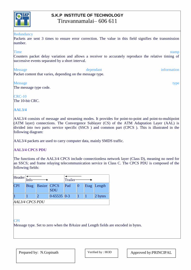
Redundancy
Packets are sent 3 times to ensure error correction. The value in this field signifies the transmission
number.
Time stamp
Counters packet delay variation and allows a receiver to accurately reproduce the relative timing of
successive events separated by a short interval.
Message dependant information
Packet content that varies, depending on the message type.
Message type
The message type code.
CRC-10
The 10-bit CRC.
AAL3/4
AAL3/4 consists of message and streaming modes. It provides for point-to-point and point-to-multipoint
(ATM layer) connections. The Convergence Sublayer (CS) of the ATM Adaptation Layer (AAL) is
divided into two parts: service specific (SSCS ) and common part (CPCS ). This is illustrated in the
following diagram:
AAL3/4 packets are used to carry computer data, mainly SMDS traffic.
AAL3/4 CPCS PDU
The functions of the AAL3/4 CPCS include connectionless network layer (Class D), meaning no need for
an SSCS; and frame relaying telecommunication service in Class C. The CPCS PDU is composed of the
following fields:
Header Info Trailer
CPI Btag Basize CPCS
SDU
Pad 0 Etag Length
1 1 2 0-65535 0-3 1 1 2 bytes
AAL3/4 CPCS PDU
CPI
Message type. Set to zero when the BAsize and Length fields are encoded in bytes.

S.K.P INSTITUTE OF TECHNOLOGY Tiruvannamalai– 606 611
Verified by : HOD Prepared by: N.Gopinath
Approved by:PRINCIPAL
Btag
Beginning tag. This is an identifier for the packet. It is repeated as the Etag.
BAsize
Buffer allocation size. Size (in bytes) that the receiver has to allocate to capture all the data.
CPCS SDU
Variable information field up to 65535 bytes.
PAD
Padding field which is used to achieve 32-bit alignment of the length of the packet.
0
All-zero.
Etag
End tag. Must be the same as Btag.
Length
Must be the same as BASize.
AAL3/4 SAR PDU
The structure of the AAL3/4 SAR PDU is illustrated below:
ST SN MID Information LI CRC
2 4 10 352 6 10 bits
2-byte header 44 bytes 2-byte trailer
48 bytes
AAL3/4 SAR PDU
ST
Segment type. Values may be as follows:
SN
Sequence number. Numbers the stream of SAR PDUs of a CPCS PDU (modulo 16).
MID
Multiplexing identification. This is used for multiplexing several AAL3/4 connections over one ATM link.

S.K.P INSTITUTE OF TECHNOLOGY Tiruvannamalai– 606 611
Verified by : HOD Prepared by: N.Gopinath
Approved by:PRINCIPAL
Information
This field has a fixed length of 44 bytes and contains parts of CPCS PDU.
LI
Length indication. Contains the length of the SAR SDU in bytes, as follows:
CRC
Cyclic redundancy check.
Functions of AAL3/4 SAR include identification of SAR SDUs; error indication and handling; SAR SDU
sequence continuity; multiplexing and demultiplexing.
AAL5 The type 5 adaptation layer is a simplified version of AAL3/4. It also consists of message and
streaming modes, with the CS divided into the service specific and common part. AAL5 provides point-to-
point and point-to-multipoint (ATM layer) connections.
AAL5 is used to carry computer data such as TCP/IP. It is the most popular AAL and is sometimes
referred to as SEAL (simple and easy adaptation layer).
AAL5 CPCS PDU
The AAL5 CPCS PDU is composed of the following fields:
Info Trailer
CPCS payload Pad UU CPI Length CRC
0-65535 0-47 1 1 2 4 bytes
AAL5 CPCS PDU
CPCS
The actual information that is sent by the user. Note that the information comes before any length
indication (as opposed to AAL3/4 where the amount of memory required is known in advance).
Pad
Padding bytes to make the entire packet (including control and CRC) fit into a 48-byte boundary.
UU
CPCS user-to-user indication to transfer one byte of user information.
CPI
Common part indicator is a filling byte (of value 0). This field is to be used in the future for layer
management message indication.

S.K.P INSTITUTE OF TECHNOLOGY Tiruvannamalai– 606 611
Verified by : HOD Prepared by: N.Gopinath
Approved by:PRINCIPAL
Length
Length of the user information without the Pad.
CRC
CRC-32. Used to allow identification of corrupted transmission.
AAL5 SAR PDU The structure of the AAL5 CS PDU is as follows:
Information PAD UU CPI Length CRC-32
1-48 0-47 1 1 2 4 bytes
8-byte trailer
AAL5 SAR PDU
High-Speed LANs Emergence of High-Speed LANs
2 Significant trends
–Computing power of PCs continues to grow rapidly
–Network computing
Examples of requirements
–Centralized server farms
–Power workgroups
–High-speed local backbone
Classical Ethernet
Bus topology LAN
10 Mbps
CSMA/CD medium access control protocol
2 problems:
–A transmission from any station can be received by all stations
–How to regulate transmission
Solution to First Problem
Data transmitted in blocks called frames:
–User data
–Frame header containing unique address of destination station
CSMA/CD
Carrier Sense Multiple Access/ Carrier Detection
If the medium is idle, transmit.
If the medium is busy, continue to listen until the channel is idle, then transmit immediately.
If a collision is detected during transmission, immediately cease transmitting.
After a collision, wait a random amount of time, then attempt to transmit again (repeat from step 1).

S.K.P INSTITUTE OF TECHNOLOGY Tiruvannamalai– 606 611
Verified by : HOD Prepared by: N.Gopinath
Approved by:PRINCIPAL
Medium Options at 10Mbps
<data rate> <signaling method> <max length>
10Base5
–10 Mbps
–50-ohm coaxial cable bus
–Maximum segment length 500 meters
10Base-T
–Twisted pair, maximum length 100 meters
–Star topology (hub or multipoint repeater at central point)

S.K.P INSTITUTE OF TECHNOLOGY Tiruvannamalai– 606 611
Verified by : HOD Prepared by: N.Gopinath
Approved by:PRINCIPAL
Hubs and Switches
Hub
Transmission from a station received by central hub and retransmitted on all outgoing lines
Only one transmission at a time
Layer 2 Switch
Incoming frame switched to one outgoing line
Many transmissions at same time
Bridge
Frame handling done in software
Analyze and forward one frame at a time
Store-and-forward
Layer 2 Switch
Frame handling done in hardware
Multiple data paths and can handle multiple frames at a time
Can do cut-through

S.K.P INSTITUTE OF TECHNOLOGY Tiruvannamalai– 606 611
Verified by : HOD Prepared by: N.Gopinath
Approved by:PRINCIPAL
Layer 2 Switches
Flat address space
Broadcast storm
Only one path between any 2 devices
Solution 1: subnetworks connected by routers
Solution 2: layer 3 switching, packet-forwarding logic in hardware
Benefits of 10 Gbps Ethernet over ATM
No expensive, bandwidth consuming conversion between Ethernet packets and ATM cells
Network is Ethernet, end to end
IP plus Ethernet offers QoS and traffic policing capabilities approach that of ATM
Wide variety of standard optical interfaces for 10 Gbps Ethernet
Fibre Channel
2 methods of communication with processor:
–I/O channel

S.K.P INSTITUTE OF TECHNOLOGY Tiruvannamalai– 606 611
Verified by : HOD Prepared by: N.Gopinath
Approved by:PRINCIPAL
–Network communications
Fibre channel combines both
–Simplicity and speed of channel communications
–Flexibility and interconnectivity of network communications

S.K.P INSTITUTE OF TECHNOLOGY Tiruvannamalai– 606 611
Verified by : HOD Prepared by: N.Gopinath
Approved by:PRINCIPAL
I/O channel
Hardware based, high-speed, short distance
Direct point-to-point or multipoint communications link
Data type qualifiers for routing payload
Link-level constructs for individual I/O operations
Protocol specific specifications to support e.g. SCSI
Fibre Channel Network-Oriented Facilities
Full multiplexing between multiple destinations
Peer-to-peer connectivity between any pair of ports
Internetworking with other connection technologies
Fibre Channel Requirements
Full duplex links with 2 fibres/link
100 Mbps – 800 Mbps
Distances up to 10 km
Small connectors
high-capacity
Greater connectivity than existing multidrop channels
Broad availability
Support for multiple cost/performance levels
Support for multiple existing interface command sets
Fibre Channel Protocol Architecture
FC-0 Physical Media
FC-1 Transmission Protocol
FC-2 Framing Protocol
FC-3 Common Services
FC-4 Mapping
Wireless LAN Requirements Throughput
Number of nodes
Connection to backbone
Service area
Battery power consumption
Transmission robustness and security
Collocated network operation
License-free operation
Handoff/roaming
Dynamic configuration
IEEE 802.11 Services
Association
Reassociation
Disassociation
Authentication

S.K.P INSTITUTE OF TECHNOLOGY Tiruvannamalai– 606 611
Verified by : HOD Prepared by: N.Gopinath
Approved by:PRINCIPAL
Privacy

S.K.P INSTITUTE OF TECHNOLOGY Tiruvannamalai– 606 611
Verified by : HOD Prepared by: N.Gopinath
Approved by:PRINCIPAL
Unit II
Queing analysis
In queuing theory, a queueing model is used to approximate a real queueing situation or system,
so the queueing behaviour can be analysed mathematically. Queueing models allow a number of
useful steady state performance measures to be determined, including:
the average number in the queue, or the system,
the average time spent in the queue, or the system,
the statistical distribution of those numbers or times,
the probability the queue is full, or empty, and
the probability of finding the system in a particular state.
These performance measures are important as issues or problems caused by queueing situations
are often related to customer dissatisfaction with service or may be the root cause of economic
losses in a business. Analysis of the relevant queueing models allows the cause of queueing
issues to be identified and the impact of any changes that might be wanted to be assessed.
Notation
Queueing models can be represented using Kendall's notation:
A/B/S/K/N/Disc
where:
A is the interarrival time distribution
B is the service time distribution
S is the number of servers
K is the system capacity
N is the calling population
Disc is the service discipline assumed
Some standard notation for distributions (A or B) are:
M for a Markovian (exponential) distribution
Eκ for an Erlang distribution with κ phases
D for Deterministic (constant)
G for General distribution
PH for a Phase-type distribution
S.K.P INSTITUTE OF TECHNOLOGY Tiruvannamalai– 606 611
Verified by : HOD Prepared by: N.Gopinath
Approved by:PRINCIPAL
Models
Construction and analysis
Queueing models are generally constructed to represent the steady state of a queueing system,
that is, the typical, long run or average state of the system. As a consequence, these are
stochastic models that represent the probability that a queueing system will be found in a
particular configuration or state.
A general procedure for constructing and analysing such queueing models is:
1. Identify the parameters of the system, such as the arrival rate, service time, Queue capacity, and
perhaps draw a diagram of the system.
2. Identify the system states. (A state will generally represent the integer number of customers,
people, jobs, calls, messages, etc. in the system and may or may not be limited.)
3. Draw a state transition diagram that represents the possible system states and identify the rates
to enter and leave each state. This diagram is a representation of a Markov chain.
4. Because the state transition diagram represents the steady state situation between state there is a
balanced flow between states so the probabilities of being in adjacent states can be related
mathematically in terms of the arrival and service rates and state probabilities.
5. Express all the state probabilities in terms of the empty state probability, using the inter-state
transition relationships.
6. Determine the empty state probability by using the fact that all state probabilities always sum to
1.
Whereas specific problems that have small finite state models are often able to be analysed
numerically, analysis of more general models, using calculus, yields useful formulae that can be
applied to whole classes of problems.
Single-server queue
Single-server queues are, perhaps, the most commonly encountered queueing situation in real
life. One encounters a queue with a single server in many situations, including business (e.g.
sales clerk), industry (e.g. a production line), transport (e.g. a bus, a taxi rank, an intersection),
telecommunications (e.g. Telephone line), computing (e.g. processor sharing). Even where there
are multiple servers handling the situation it is possible to consider each server individually as
part of the larger system, in many cases. (e.g A supermarket checkout has several single server
queues that the customer can select from.) Consequently, being able to model and analyse a
single server queue's behaviour is a particularly useful thing to do.
Poisson arrivals and service
M/M/1/∞/∞ represents a single server that has unlimited queue capacity and infinite calling
population, both arrivals and service are Poisson (or random) processes, meaning the statistical
distribution of both the inter-arrival times and the service times follow the exponential
distribution. Because of the mathematical nature of the exponential distribution, a number of

S.K.P INSTITUTE OF TECHNOLOGY Tiruvannamalai– 606 611
Verified by : HOD Prepared by: N.Gopinath
Approved by:PRINCIPAL
quite simple relationships are able to be derived for several performance measures based on
knowing the arrival rate and service rate.
This is fortunate because, an M/M/1 queuing model can be used to approximate many queuing
situations.
Poisson arrivals and general service
M/G/1/∞/∞ represents a single server that has unlimited queue capacity and infinite calling
population, while the arrival is still Poisson process, meaning the statistical distribution of the
inter-arrival times still follow the exponential distribution, the distribution of the service time
does not. The distribution of the service time may follow any general statistical distribution, not
just exponential. Relationships are still able to be derived for a (limited) number of performance
measures if one knows the arrival rate and the mean and variance of the service rate. However
the derivations a generally more complex.
A number of special cases of M/G/1 provide specific solutions that give broad insights into the
best model to choose for specific queueing situations because they permit the comparison of
those solutions to the performance of an M/M/1 model.
Multiple-servers queue
Multiple (identical)-servers queue situations are frequently encountered in telecommunications
or a customer service environment. When modelling these situations care is needed to ensure
that it is a multiple servers queue, not a network of single server queues, because results may
differ depending on how the queuing model behaves.
One observational insight provided by comparing queuing models is that a single queue with
multiple servers performs better than each server having their own queue and that a single large
pool of servers performs better than two or more smaller pools, even though there are the same
total number of servers in the system.
One simple example to prove the above fact is as follows: Consider a system having 8 input
lines, single queue and 8 servers.The output line has a capacity of 64 kbit/s. Considering the
arrival rate at each input as 2 packets/s. So, the total arrival rate is 16 packets/s. With an average
of 2000 bits per packet, the service rate is 64 kbit/s/2000b = 32 packets/s. Hence, the average
response time of the system is 1/(μ-λ) = 1/(32-16) = 0.0667 sec. Now, consider a second system
with 8 queues, one for each server. Each of the 8 output lines has a capacity of 8 kbit/s. The
calculation yields the response time as 1/(μ-λ) = 1/(4-2) = 0.5 sec. And the average waiting time
in the queue in the first case is ρ/(1-ρ)μ = 0.25, while in the second case is 0.03125.
Infinitely many servers
While never exactly encountered in reality, an infinite-servers (e.g. M/M/∞) model is a
convenient theoretical model for situations that involve storage or delay, such as parking lots,

S.K.P INSTITUTE OF TECHNOLOGY Tiruvannamalai– 606 611
Verified by : HOD Prepared by: N.Gopinath
Approved by:PRINCIPAL
warehouses and even atomic transitions. In these models there is no queue, as such, instead each
arriving customer receives service. When viewed from the outside, the model appears to delay
or store each customer for some time.
Queueing System Classification
With Little's Theorem, we have developed some basic understanding of a queueing system. To
further our understanding we will have to dig deeper into characteristics of a queueing system
that impact its performance. For example, queueing requirements of a restaurant will depend
upon factors like:
How do customers arrive in the restaurant? Are customer arrivals more during lunch and dinner
time (a regular restaurant)? Or is the customer traffic more uniformly distributed (a cafe)?
How much time do customers spend in the restaurant? Do customers typically leave the
restaurant in a fixed amount of time? Does the customer service time vary with the type of
customer?
How many tables does the restaurant have for servicing customers?
The above three points correspond to the most important characteristics of a queueing system.
They are explained below:
Arrival Process The probability density distribution that determines the
customer arrivals in the system.
In a messaging system, this refers to the message arrival
probability distribution.
Service Process The probability density distribution that determines the
customer service times in the system.
In a messaging system, this refers to the message transmission
time distribution. Since message transmission is directly
proportional to the length of the message, this parameter
indirectly refers to the message length distribution.
Number of Servers Number of servers available to service the customers.
In a messaging system, this refers to the number of links
between the source and destination nodes.
Based on the above characteristics, queueing systems can be classified by the following
convention:
A/S/n

S.K.P INSTITUTE OF TECHNOLOGY Tiruvannamalai– 606 611
Verified by : HOD Prepared by: N.Gopinath
Approved by:PRINCIPAL
Where A is the arrival process, S is the service process and n is the number of servers. A and S
are can be any of the following:
M (Markov) Exponential probability density
D (Deterministic) All customers have the same value
G (General) Any arbitrary probability distribution
Examples of queueing systems that can be defined with this convention are:
M/M/1: This is the simplest queueing system to analyze. Here the arrival and service time are
negative exponentially distributed (poisson process). The system consists of only one server.
This queueing system can be applied to a wide variety of problems as any system with a very
large number of independent customers can be approximated as a Poisson process. Using a
Poisson process for service time however is not applicable in many applications and is only a
crude approximation. Refer to M/M/1 Queueing System for details.
M/D/n: Here the arrival process is poisson and the service time distribution is deterministic. The
system has n servers. (e.g. a ticket booking counter with n cashiers.) Here the service time can
be assumed to be same for all customers)
G/G/n: This is the most general queueing system where the arrival and service time processes
are both arbitrary. The system has n servers. No analytical solution is known for this queueing
system.
Markovian arrival processes
In queuing theory, Markovian arrival processes are used to model the arrival customers to
queue.
Some of the most common include the Poisson process, Markovian arrival process and the
batch Markovian arrival process.
Markovian arrival processes has two processes. A continuous-time Markov process j(t), a
Markov process which is generated by a generator or rate matrix, Q. The other process is a
counting process N(t), which has state space (where is the set of all
natural numbers). N(t) increases every time there is a transition in j(t) which marked.
Poisson process
The Poisson arrival process or Poisson process counts the number of arrivals, each of which has
a exponentially distributed time between arrival. In the most general case this can be represented
by the rate matrix,

S.K.P INSTITUTE OF TECHNOLOGY Tiruvannamalai– 606 611
Verified by : HOD Prepared by: N.Gopinath
Approved by:PRINCIPAL
Markov arrival process
The Markov arrival process (MAP) is a generalisation of the Poisson process by having non-
exponential distribution sojourn between arrivals. The homogeneous case has rate matrix,
Little's law
In queueing theory, Little's result, theorem, lemma, or law says:
The average number of customers in a stable system (over some time interval), N, is equal to
their average arrival rate, λ, multiplied by their average time in the system, T, or:
Although it looks intuitively reasonable, it's a quite remarkable result, as it implies that this
behavior is entirely independent of any of the detailed probability distributions involved, and
hence requires no assumptions about the schedule according to which customers arrive or are
serviced, or whether they are served in the order in which they arrive.
It is also a comparatively recent result - it was first proved by John Little, an Institute Professor
and the Chair of Management Science at the MIT Sloan School of Management, in 1961.
Handily his result applies to any system, and particularly, it applies to systems within systems.
So in a bank, the queue might be one subsystem, and each of the tellers another subsystem, and
Little's result could be applied to each one, as well as the whole thing. The only requirement is
that the system is stable -- it can't be in some transition state such as just starting up or just
shutting down.
Mathematical formalization of Little's theorem
Let α(t) be to some system in the interval [0, t]. Let β(t) be the number of departures from the
same system in the interval [0, t]. Both α(t) and β(t) are integer valued increasing functions by
their definition. Let Tt be the mean time spent in the system (during the interval [0, t]) for all the
customers who were in the system during the interval [0, t]. Let Nt be the mean number of
customers in the system over the duration of the interval [0, t].
If the following limits exist,

S.K.P INSTITUTE OF TECHNOLOGY Tiruvannamalai– 606 611
Verified by : HOD Prepared by: N.Gopinath
Approved by:PRINCIPAL
and, further, if λ = δ then Little's theorem holds, the limit
exists and is given by Little's theorem,
Ideal Performance

S.K.P INSTITUTE OF TECHNOLOGY Tiruvannamalai– 606 611
Verified by : HOD Prepared by: N.Gopinath
Approved by:PRINCIPAL
Effects of Congestion
‘
Congestion-Control Mechanisms
Backpressure
– Request from destination to source to reduce rate
– Useful only on a logical connection basis
– Requires hop-by-hop flow control mechanism
Policing
– Measuring and restricting packets as they enter the network
Choke packet
– Specific message back to source
– E.g., ICMP Source Quench
Implicit congestion signaling
– Source detects congestion from transmission delays and lost packets and reduces flow
S.K.P INSTITUTE OF TECHNOLOGY Tiruvannamalai– 606 611
Verified by : HOD Prepared by: N.Gopinath
Approved by:PRINCIPAL
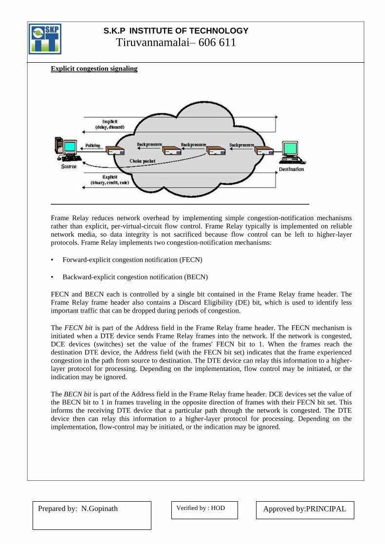
Explicit congestion signaling
Frame Relay reduces network overhead by implementing simple congestion-notification mechanisms
rather than explicit, per-virtual-circuit flow control. Frame Relay typically is implemented on reliable
network media, so data integrity is not sacrificed because flow control can be left to higher-layer
protocols. Frame Relay implements two congestion-notification mechanisms:
• Forward-explicit congestion notification (FECN)
• Backward-explicit congestion notification (BECN)
FECN and BECN each is controlled by a single bit contained in the Frame Relay frame header. The
Frame Relay frame header also contains a Discard Eligibility (DE) bit, which is used to identify less
important traffic that can be dropped during periods of congestion.
The FECN bit is part of the Address field in the Frame Relay frame header. The FECN mechanism is
initiated when a DTE device sends Frame Relay frames into the network. If the network is congested,
DCE devices (switches) set the value of the frames' FECN bit to 1. When the frames reach the
destination DTE device, the Address field (with the FECN bit set) indicates that the frame experienced
congestion in the path from source to destination. The DTE device can relay this information to a higher-
layer protocol for processing. Depending on the implementation, flow control may be initiated, or the
indication may be ignored.
The BECN bit is part of the Address field in the Frame Relay frame header. DCE devices set the value of
the BECN bit to 1 in frames traveling in the opposite direction of frames with their FECN bit set. This
informs the receiving DTE device that a particular path through the network is congested. The DTE
device then can relay this information to a higher-layer protocol for processing. Depending on the
implementation, flow-control may be initiated, or the indication may be ignored.

S.K.P INSTITUTE OF TECHNOLOGY Tiruvannamalai– 606 611
Verified by : HOD Prepared by: N.Gopinath
Approved by:PRINCIPAL
Frame Relay Discard Eligibility
The Discard Eligibility (DE) bit is used to indicate that a frame has lower importance than other frames.
The DE bit is part of the Address field in the Frame Relay frame header.
DTE devices can set the value of the DE bit of a frame to 1 to indicate that the frame has lower
importance than other frames. When the network becomes congested, DCE devices will discard frames
with the DE bit set before discarding those that do not. This reduces the likelihood of critical data being
dropped by Frame Relay DCE devices during periods of congestion.
Frame Relay Error Checking
Frame Relay uses a common error-checking mechanism known as the cyclic redundancy check (CRC).
The CRC compares two calculated values to determine whether errors occurred during the transmission
from source to destination. Frame Relay reduces network overhead by implementing error checking
rather than error correction. Frame Relay typically is implemented on reliable network media, so data
integrity is not sacrificed because error correction can be left to higher-layer protocols running on top of
Frame Relay.
Traffic Management in Congested Network – Some Considerations
Fairness
– Various flows should “suffer” equally
– Last-in-first-discarded may not be fair
Quality of Service (QoS)
– Flows treated differently, based on need
– Voice, video: delay sensitive, loss insensitive
– File transfer, mail: delay insensitive, loss sensitive
– Interactive computing: delay and loss sensitive
Reservations
– Policing: excess traffic discarded or handled on best-effort basis
–
Frame Relay Congestion Control
Minimize frame discard
Maintain QoS (per-connection bandwidth)
Minimize monopolization of network
Simple to implement, little overhead
Minimal additional network traffic
Resources distributed fairly
Limit spread of congestion
Operate effectively regardless of flow

S.K.P INSTITUTE OF TECHNOLOGY Tiruvannamalai– 606 611
Verified by : HOD Prepared by: N.Gopinath
Approved by:PRINCIPAL
Have minimum impact other systems in network
Minimize variance in QoS
Congestion Avoidance with Explicit Signaling
Two general strategies considered:
Hypothesis 1: Congestion always occurs slowly, almost always at egress nodes
– forward explicit congestion avoidance
Hypothesis 2: Congestion grows very quickly in internal nodes and requires quick action
– backward explicit congestion avoidance
Explicit Signaling Response
Network Response
– each frame handler monitors its queuing behavior and takes action
– use FECN/BECN bits
– some/all connections notified of congestion
User (end-system) Response
– receipt of BECN/FECN bits in frame
– BECN at sender: reduce transmission rate
– FECN at receiver: notify peer (via LAPF or higher layer) to restrict flow
Frame Relay Traffic Rate Management Parameters
Committed Information Rate (CIR)
– Average data rate in bits/second that the network agrees to support for a connection
Data Rate of User Access Channel (Access Rate)
– Fixed rate link between user and network (for network access)

S.K.P INSTITUTE OF TECHNOLOGY Tiruvannamalai– 606 611
Verified by : HOD Prepared by: N.Gopinath
Approved by:PRINCIPAL
Committed Burst Size (Bc)
– Maximum data over an interval agreed to by network
Excess Burst Size (Be)
– Maximum data, above Bc, over an interval that network will attempt to transfer
Relationship of Congestion Parameters

S.K.P INSTITUTE OF TECHNOLOGY Tiruvannamalai– 606 611
Verified by : HOD Prepared by: N.Gopinath
Approved by:PRINCIPAL
Unit III
TCP Flow Control Uses a form of sliding window
Differs from mechanism used in LLC, HDLC, X.25, and others:
Decouples acknowledgement of received data units from granting permission to
send more
TCP’s flow control is known as a credit allocation scheme:
Each transmitted octet is considered to have a sequence number
TCP Header Fields for Flow Control
Sequence number (SN) of first octet in data segment
Acknowledgement number (AN)
Window (W)
Acknowledgement contains AN = i, W = j:
Octets through SN = i - 1 acknowledged
Permission is granted to send W = j more octets,
i.e., octets i through i + j - 1
TCP Credit Allocation Mechanism

S.K.P INSTITUTE OF TECHNOLOGY Tiruvannamalai– 606 611
Verified by : HOD Prepared by: N.Gopinath
Approved by:PRINCIPAL
Credit Allocation is Flexible
Suppose last message B issued was AN = i, W = j
To increase credit to k (k > j) when no new data, B issues AN = i, W = k
To acknowledge segment containing m octets (m < j), B issues AN = i + m, W = j – m
Flow Control Perspectives

S.K.P INSTITUTE OF TECHNOLOGY Tiruvannamalai– 606 611
Verified by : HOD Prepared by: N.Gopinath
Approved by:PRINCIPAL
Credit Policy
Receiver needs a policy for how much credit to give sender
Conservative approach: grant credit up to limit of available buffer space
May limit throughput in long-delay situations
Optimistic approach: grant credit based on expectation of freeing space before data arrives
Effect of Window Size
W = TCP window size (octets)
R = Data rate (bps) at TCP source
D = Propagation delay (seconds)
After TCP source begins transmitting, it takes D seconds for first octet to arrive, and D seconds for
acknowledgement to return
TCP source could transmit at most 2RD bits, or RD/4 octets
Normalized Throughput S
1 W > RD / 4
S =
4W/RD W < RD / 4
Window Scale Parameter
Complicating Factors
Multiple TCP connections are multiplexed over same network interface, reducing R and efficiency
For multi-hop connections, D is the sum of delays across each network plus delays at each router
If source data rate R exceeds data rate on one of the hops, that hop will be a bottleneck
Lost segments are retransmitted, reducing throughput. Impact depends on retransmission policy

S.K.P INSTITUTE OF TECHNOLOGY Tiruvannamalai– 606 611
Verified by : HOD Prepared by: N.Gopinath
Approved by:PRINCIPAL
Retransmission Strategy
TCP relies exclusively on positive acknowledgements and retransmission on acknowledgement timeout
There is no explicit negative acknowledgement
Retransmission required when:
Segment arrives damaged, as indicated by checksum error, causing receiver to discard segment
Segment fails to arrive
Timers
A timer is associated with each segment as it is sent
If timer expires before segment acknowledged, sender must retransmit
Key Design Issue:
value of retransmission timer
Too small: many unnecessary retransmissions, wasting network bandwidth
Too large: delay in handling lost segment
Two Strategies
Timer should be longer than round-trip delay (send segment, receive ack)
Delay is variable
Strategies:
Fixed timer
Adaptive
Problems with Adaptive Scheme
Peer TCP entity may accumulate acknowledgements and not acknowledge immediately
For retransmitted segments, can’t tell whether acknowledgement is response to original transmission or
retransmission
Network conditions may change suddenly
Adaptive Retransmission Timer
Average Round-Trip Time (ARTT)
K + 1
ARTT(K + 1) = 1 ∑ RTT(i)
K + 1 i = 1
= K ART(K) + 1 RTT(K + 1)
K + 1 K + 1
RFC 793 Exponential Averaging
Smoothed Round-Trip Time (SRTT)

S.K.P INSTITUTE OF TECHNOLOGY Tiruvannamalai– 606 611
Verified by : HOD Prepared by: N.Gopinath
Approved by:PRINCIPAL
SRTT(K + 1) = α × SRTT(K)
+ (1 – α) × SRTT(K + 1)
The older the observation, the less it is counted in the average.
RFC 793 Retransmission Timeout
RTO(K + 1) =
Min(UB, Max(LB, β × SRTT(K + 1)))
UB, LB: prechosen fixed upper and lower bounds
Example values for α, β:
0.8 < α < 0.9 1.3 < β < 2.0
Implementation Policy Options
Send
Deliver
Accept
In-order
In-window
Retransmit
First-only
Batch
individual
Acknowledge
immediate
cumulative
TCP Congestion Control
Dynamic routing can alleviate congestion by spreading load more evenly
But only effective for unbalanced loads and brief surges in traffic
Congestion can only be controlled by limiting total amount of data entering network
ICMP source Quench message is crude and not effective
RSVP may help but not widely implemented
TCP Congestion Control is Difficult
IP is connectionless and stateless, with no provision for detecting or controlling congestion
TCP only provides end-to-end flow control
No cooperative, distributed algorithm to bind together various TCP entities
TCP Flow and Congestion Control

S.K.P INSTITUTE OF TECHNOLOGY Tiruvannamalai– 606 611
Verified by : HOD Prepared by: N.Gopinath
Approved by:PRINCIPAL
The rate at which a TCP entity can transmit is determined by rate of incoming ACKs to previous
segments with new credit
Rate of Ack arrival determined by round-trip path between source and destination
Bottleneck may be destination or internet
Sender cannot tell which
Only the internet bottleneck can be due to congestion
TCP Segment Pacing
TCP Flow and Congestion Control

S.K.P INSTITUTE OF TECHNOLOGY Tiruvannamalai– 606 611
Verified by : HOD Prepared by: N.Gopinath
Approved by:PRINCIPAL
Retransmission Timer Management
Three Techniques to calculate retransmission timer (RTO):
RTT Variance Estimation
Exponential RTO Backoff
Karn’s Algorithm
RTT Variance Estimation
(Jacobson’s Algorithm)
3 sources of high variance in RTT
If data rate relative low, then transmission delay will be relatively large, with larger variance due to
variance in packet size
Load may change abruptly due to other sources
Peer may not acknowledge segments immediately
Jacobson’s Algorithm
SRTT(K + 1) = (1 – g) × SRTT(K) + g × RTT(K + 1)
SERR(K + 1) = RTT(K + 1) – SRTT(K)
SDEV(K + 1) = (1 – h) × SDEV(K) + h ×|SERR(K + 1)|
RTO(K + 1) = SRTT(K + 1) + f × SDEV(K + 1)
g = 0.125
h = 0.25
f = 2 or f = 4 (most current implementations use f = 4)
Two Other Factors
Jacobson’s algorithm can significantly improve TCP performance, but:
What RTO to use for retransmitted segments?
ANSWER: exponential RTO backoff algorithm
Which round-trip samples to use as input to Jacobson’s algorithm?
ANSWER: Karn’s algorithm
Exponential RTO Backoff
Increase RTO each time the same segment retransmitted – backoff process
Multiply RTO by constant:
RTO = q × RTO
q = 2 is called binary exponential backoff
Which Round-trip Samples?

S.K.P INSTITUTE OF TECHNOLOGY Tiruvannamalai– 606 611
Verified by : HOD Prepared by: N.Gopinath
Approved by:PRINCIPAL
If an ack is received for retransmitted segment, there are 2 possibilities:
Ack is for first transmission
Ack is for second transmission
TCP source cannot distinguish 2 cases
No valid way to calculate RTT:
–From first transmission to ack, or
–From second transmission to ack?
–Karn’s Algorithm
Do not use measured RTT to update SRTT and SDEV
Calculate backoff RTO when a retransmission occurs
Use backoff RTO for segments until an ack arrives for a segment that has not been retransmitted
Then use Jacobson’s algorithm to calculate RTO
Window Management
Slow start
Dynamic window sizing on congestion
Fast retransmit
Fast recovery
Limited transmit
Slow Start
awnd = MIN[ credit, cwnd]
where
awnd = allowed window in segments
cwnd = congestion window in segments
credit = amount of unused credit granted in most recent ack
cwnd = 1 for a new connection and increased by 1 for each ack received, up to a maximum

S.K.P INSTITUTE OF TECHNOLOGY Tiruvannamalai– 606 611
Verified by : HOD Prepared by: N.Gopinath
Approved by:PRINCIPAL
Effect of Slow Start
Dynamic Window Sizing on Congestion
A lost segment indicates congestion
Prudent to reset cwsd = 1 and begin slow start process
May not be conservative enough: “ easy to drive a network into saturation but hard for the net to
recover” (Jacobson)
Instead, use slow start with linear growth in cwnd
Illustration of Slow Start and Congestion Avoidance

S.K.P INSTITUTE OF TECHNOLOGY Tiruvannamalai– 606 611
Verified by : HOD Prepared by: N.Gopinath
Approved by:PRINCIPAL
Fast Retransmit
RTO is generally noticeably longer than actual RTT
If a segment is lost, TCP may be slow to retransmit
TCP rule: if a segment is received out of order, an ack must be issued immediately for the last in-order
segment
Fast Retransmit rule: if 4 acks received for same segment, highly likely it was lost, so retransmit
immediately, rather than waiting for timeout
Fast Recovery
When TCP retransmits a segment using Fast Retransmit, a segment was assumed lost
Congestion avoidance measures are appropriate at this point
E.g., slow-start/congestion avoidance procedure
This may be unnecessarily conservative since multiple acks indicate segments are getting through
Fast Recovery: retransmit lost segment, cut cwnd in half, proceed with linear increase of cwnd
This avoids initial exponential slow-start
Limited Transmit
If congestion window at sender is small, fast retransmit may not get triggered, e.g., cwnd = 3
Under what circumstances does sender have small congestion window?
Is the problem common?
If the problem is common, why not reduce number of duplicate acks needed to trigger retransmit?
Limited Transmit Algorithm
Sender can transmit new segment when 3 conditions are met:
Two consecutive duplicate acks are received
Destination advertised window allows transmission of segment
Amount of outstanding data after sending is less than or equal to cwnd + 2
Performance of TCP over ATM
How best to manage TCP’s segment size, window management and congestion control…
…at the same time as ATM’s quality of service and traffic control policies
TCP may operate end-to-end over one ATM network, or there may be multiple ATM LANs or WANs
with non-ATM networks
TCP/IP over AAL5/ATM
S.K.P INSTITUTE OF TECHNOLOGY Tiruvannamalai– 606 611
Verified by : HOD Prepared by: N.Gopinath
Approved by:PRINCIPAL
Performance of TCP over UBR
Buffer capacity at ATM switches is a critical parameter in assessing TCP throughput performance
Insufficient buffer capacity results in lost TCP segments and retransmissions
Effect of Switch Buffer Size
Data rate of 141 Mbps
End-to-end propagation delay of 6 μs
IP packet sizes of 512 octets to 9180
TCP window sizes from 8 Kbytes to 64 Kbytes
ATM switch buffer size per port from 256 cells to 8000
One-to-one mapping of TCP connections to ATM virtual circuits
TCP sources have infinite supply of data ready
Observations
If a single cell is dropped, other cells in the same IP datagram are unusable, yet ATM network forwards
these useless cells to destination
Smaller buffer increase probability of dropped cells
Larger segment size increases number of useless cells transmitted if a single cell dropped
Partial Packet and Early Packet Discard
Reduce the transmission of useless cells
Work on a per-virtual circuit basis
Partial Packet Discard
–If a cell is dropped, then drop all subsequent cells in that segment (i.e., look for cell with SDU type bit set
to one)
Early Packet Discard
–When a switch buffer reaches a threshold level, preemptively discard all cells in a segment
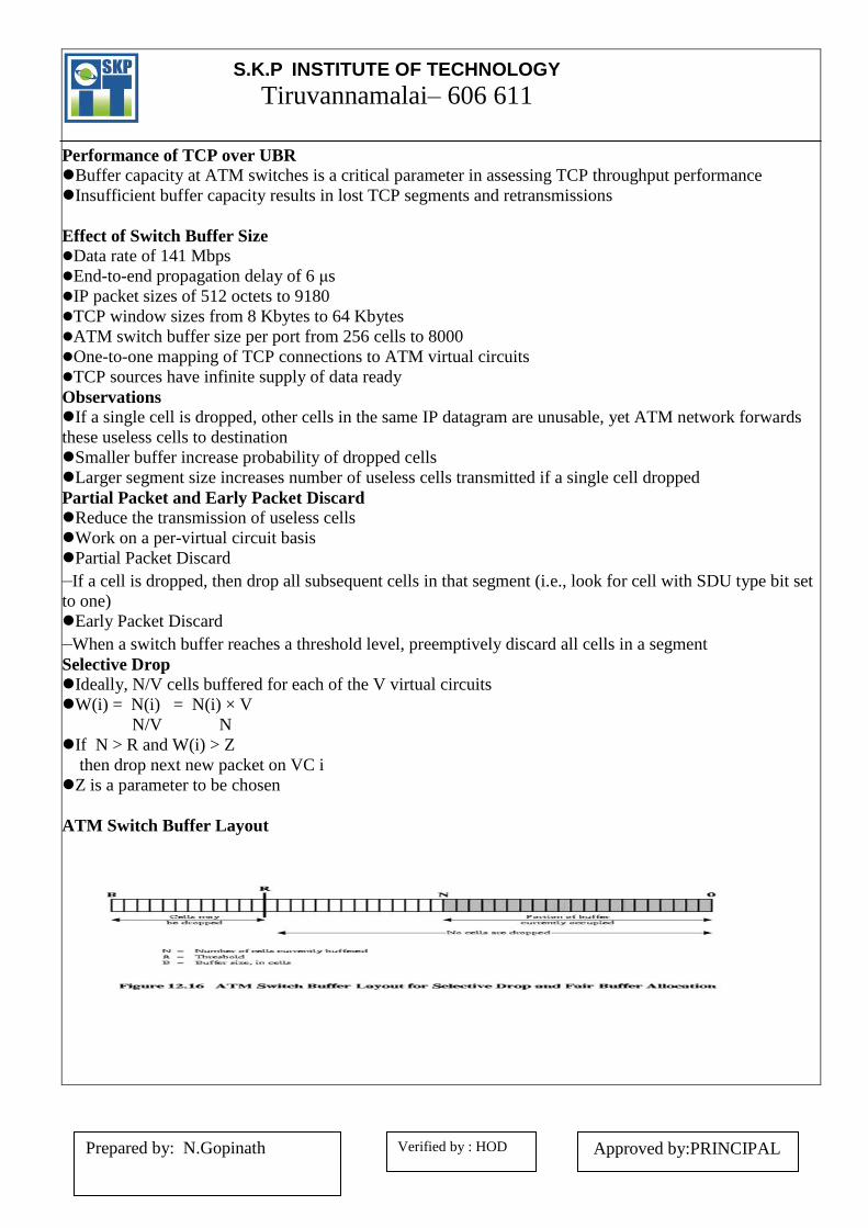
Selective Drop
Ideally, N/V cells buffered for each of the V virtual circuits
W(i) = N(i) = N(i) × V
N/V N
If N > R and W(i) > Z
then drop next new packet on VC i
Z is a parameter to be chosen
ATM Switch Buffer Layout

S.K.P INSTITUTE OF TECHNOLOGY Tiruvannamalai– 606 611
Verified by : HOD Prepared by: N.Gopinath
Approved by:PRINCIPAL
Fair Buffer Allocation
More aggressive dropping of packets as congestion increases
Drop new packet when:
N > R and W(i) > Z × B – R
N - R
TCP over ABR
Good performance of TCP over UBR can be achieved with minor adjustments to switch mechanisms
This reduces the incentive to use the more complex and more expensive ABR service
Performance and fairness of ABR quite sensitive to some ABR parameter settings
Overall, ABR does not provide significant performance over simpler and less expensive UBR-EPD or
UBR-EPD-FBA
Traffic and Congestion Control in ATM Networks Introduction
Control needed to prevent switch buffer overflow
High speed and small cell size gives different problems from other networks
Limited number of overhead bits
ITU-T specified restricted initial set
– I.371
ATM forum Traffic Management Specification 41
Overview
Congestion problem
Framework adopted by ITU-T and ATM forum
– Control schemes for delay sensitive traffic
Voice & video
– Not suited to bursty traffic
– Traffic control
– Congestion control
Bursty traffic
– Available Bit Rate (ABR)
– Guaranteed Frame Rate (GFR)
Requirements for ATM Traffic and Congestion Control
Most packet switched and frame relay networks carry non-real-time bursty data
– No need to replicate timing at exit node
– Simple statistical multiplexing
– User Network Interface capacity slightly greater than average of channels
Congestion control tools from these technologies do not work in ATM
Problems with ATM Congestion Control
Most traffic not amenable to flow control
– Voice & video can not stop generating

S.K.P INSTITUTE OF TECHNOLOGY Tiruvannamalai– 606 611
Verified by : HOD Prepared by: N.Gopinath
Approved by:PRINCIPAL
Feedback slow
– Small cell transmission time v propagation delay
Wide range of applications
– From few kbps to hundreds of Mbps
– Different traffic patterns
– Different network services
High speed switching and transmission
– Volatile congestion and traffic control
Key Performance Issues-Latency/Speed Effects
E.g. data rate 150Mbps
Takes (53 x 8 bits)/(150 x 106) =2.8 x 10⁻⁶ seconds to insert a cell
Transfer time depends on number of intermediate switches, switching time and propagation delay.
Assuming no switching delay and speed of light propagation, round trip delay of 48 x 10-3 sec
across USA
A dropped cell notified by return message will arrive after source has transmitted N further cells
N=(48 x 10-3 seconds)/(2.8 x 10-6 seconds per cell)
=1.7 x 10⁴ cells = 7.2 x 106 bits
i.e. over 7 Mbits
Cell Delay Variation
For digitized voice delay across network must be small
Rate of delivery must be constant
Variations will occur
Dealt with by Time Reassembly of CBR cells (see next slide)
Results in cells delivered at CBR with occasional gaps due to dropped cells
Subscriber requests minimum cell delay variation from network provider
– Increase data rate at UNI relative to load
– Increase resources within network
Time Reassembly of CBR Cells

S.K.P INSTITUTE OF TECHNOLOGY Tiruvannamalai– 606 611
Verified by : HOD Prepared by: N.Gopinath
Approved by:PRINCIPAL
Network Contribution to Cell Delay Variation
In packet switched network
– Queuing effects at each intermediate switch
– Processing time for header and routing
Less for ATM networks
– Minimal processing overhead at switches
Fixed cell size, header format
No flow control or error control processing
– ATM switches have extremely high throughput
– Congestion can cause cell delay variation
Build up of queuing effects at switches
Total load accepted by network must be controlled
Cell Delay Variation at UNI
Caused by processing in three layers of ATM model
– See next slide for details
None of these delays can be predicted
None follow repetitive pattern
So, random element exists in time interval between reception by ATM stack and transmission
ATM Traffic-Related Attributes
Six service categories (see chapter 5)
– Constant bit rate (CBR)
– Real time variable bit rate (rt-VBR)
– Non-real-time variable bit rate (nrt-VBR)
– Unspecified bit rate (UBR)
– Available bit rate (ABR)
– Guaranteed frame rate (GFR)
Characterized by ATM attributes in four categories
– Traffic descriptors
– QoS parameters
– Congestion
– Other
Traffic Parameters
Traffic pattern of flow of cells
– Intrinsic nature of traffic
Source traffic descriptor
– Modified inside network
Connection traffic descriptor
Source Traffic Descriptor Peak cell rate
– Upper bound on traffic that can be submitted
– Defined in terms of minimum spacing between cells T
– PCR = 1/T
– Mandatory for CBR and VBR services
Sustainable cell rate
S.K.P INSTITUTE OF TECHNOLOGY Tiruvannamalai– 606 611
Verified by : HOD Prepared by: N.Gopinath
Approved by:PRINCIPAL
– Upper bound on average rate
– Calculated over large time scale relative to T
– Required for VBR
– Enables efficient allocation of network resources between VBR sources
– Only useful if SCR < PCR
Maximum burst size
– Max number of cells that can be sent at PCR
– If bursts are at MBS, idle gaps must be enough to keep overall rate below SCR
– Required for VBR
Minimum cell rate
– Min commitment requested of network
– Can be zero
– Used with ABR and GFR
– ABR & GFR provide rapid access to spare network capacity up to PCR
– PCR – MCR represents elastic component of data flow
– Shared among ABR and GFR flows
Maximum frame size
– Max number of cells in frame that can be carried over GFR connection
– Only relevant in GFR
Connection Traffic Descriptor
Includes source traffic descriptor plus:-
Cell delay variation tolerance
Amount of variation in cell delay introduced by network interface and UNI
Bound on delay variability due to slotted nature of ATM, physical layer overhead and layer
functions (e.g. cell multiplexing)
Represented by time variable τ
Conformance definition
Specify conforming cells of connection at UNI
Enforced by dropping or marking cells over definition
Quality of Service Parameters-maxCTD
Cell transfer delay (CTD)
Time between transmission of first bit of cell at source and reception of last bit at destination
Typically has probability density function (see next slide)
Fixed delay due to propagation etc.
Cell delay variation due to buffering and scheduling
Maximum cell transfer delay (maxCTD)is max requested delay for connection
Fraction α of cells exceed threshold
Discarded or delivered late
Peak-to-peak CDV & CLR
Peak-to-peak Cell Delay Variation
Remaining (1-α) cells within QoS
Delay experienced by these cells is between fixed delay and maxCTD
This is peak-to-peak CDV
CDVT is an upper bound on CDV

S.K.P INSTITUTE OF TECHNOLOGY Tiruvannamalai– 606 611
Verified by : HOD Prepared by: N.Gopinath
Approved by:PRINCIPAL
Cell loss ratio
Ratio of cells lost to cells transmitted
Cell Transfer Delay PDF
Congestion Control Attributes
Only feedback is defined
ABR and GFR
Actions taken by network and end systems to regulate traffic submitted
ABR flow control
Adaptively share available bandwidth
Other Attributes
Behaviour class selector (BCS)
– Support for IP differentiated services (chapter 16)
– Provides different service levels among UBR connections
– Associate each connection with a behaviour class
– May include queuing and scheduling
Minimum desired cell rate
Traffic Management Framework
Objectives of ATM layer traffic and congestion control
– Support QoS for all foreseeable services
– Not rely on network specific AAL protocols nor higher layer application specific protocols
– Minimize network and end system complexity
– Maximize network utilization
Timing Levels
Cell insertion time
Round trip propagation time
Connection duration

S.K.P INSTITUTE OF TECHNOLOGY Tiruvannamalai– 606 611
Verified by : HOD Prepared by: N.Gopinath
Approved by:PRINCIPAL
Long term
Traffic Control and Congestion Functions
Traffic Control Strategy
Determine whether new ATM connection can be accommodated
Agree performance parameters with subscriber
Traffic contract between subscriber and network
This is congestion avoidance
If it fails congestion may occur
– Invoke congestion control
Traffic Control
Resource management using virtual paths
Connection admission control
Usage parameter control
Selective cell discard
Traffic shaping
Explicit forward congestion indication
Resource Management Using Virtual Paths
Allocate resources so that traffic is separated according to service characteristics
Virtual path connection (VPC) are groupings of virtual channel connections (VCC)
Applications
User-to-user applications
– VPC between UNI pair
– No knowledge of QoS for individual VCC

S.K.P INSTITUTE OF TECHNOLOGY Tiruvannamalai– 606 611
Verified by : HOD Prepared by: N.Gopinath
Approved by:PRINCIPAL
– User checks that VPC can take VCCs’ demands
User-to-network applications
– VPC between UNI and network node
– Network aware of and accommodates QoS of VCCs
Network-to-network applications
– VPC between two network nodes
– Network aware of and accommodates QoS of VCCs
Resource Management Concerns
Cell loss ratio
Max cell transfer delay
Peak to peak cell delay variation
All affected by resources devoted to VPC
If VCC goes through multiple VPCs, performance depends on consecutive VPCs and on node
performance
– VPC performance depends on capacity of VPC and traffic characteristics of VCCs
– VCC related function depends on switching/processing speed and priority
VCCs and VPCs Configuration
Allocation of Capacity to VPC
Aggregate peak demand
– May set VPC capacity (data rate) to total of VCC peak rates
Each VCC can give QoS to accommodate peak demand
VPC capacity may not be fully used
Statistical multiplexing
– VPC capacity >= average data rate of VCCs but < aggregate peak demand

S.K.P INSTITUTE OF TECHNOLOGY Tiruvannamalai– 606 611
Verified by : HOD Prepared by: N.Gopinath
Approved by:PRINCIPAL
– Greater CDV and CTD
– May have greater CLR
– More efficient use of capacity
– For VCCs requiring lower QoS
– Group VCCs of similar traffic together
Connection Admission Control
User must specify service required in both directions
– Category
– Connection traffic descriptor
Source traffic descriptor
CDVT
Requested conformance definition
– QoS parameter requested and acceptable value
Network accepts connection only if it can commit resources to support requests
Procedures to Set Traffic Control Parameters
Cell Loss Priority
Two levels requested by user
– Priority for individual cell indicated by CLP bit in header
– If two levels are used, traffic parameters for both flows specified
High priority CLP = 0
All traffic CLP = 0 + 1
– May improve network resource allocation
Usage Parameter Control
UPC
Monitors connection for conformity to traffic contract
Protect network resources from overload on one connection
Done at VPC or VCC level
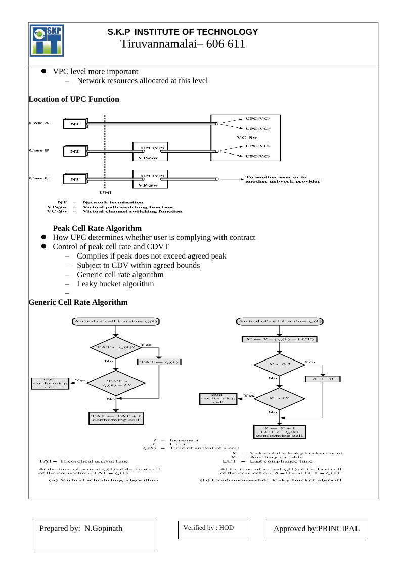
S.K.P INSTITUTE OF TECHNOLOGY Tiruvannamalai– 606 611
Verified by : HOD Prepared by: N.Gopinath
Approved by:PRINCIPAL
VPC level more important
– Network resources allocated at this level
Location of UPC Function
Peak Cell Rate Algorithm
How UPC determines whether user is complying with contract
Control of peak cell rate and CDVT
– Complies if peak does not exceed agreed peak
– Subject to CDV within agreed bounds
– Generic cell rate algorithm
– Leaky bucket algorithm
–
Generic Cell Rate Algorithm

S.K.P INSTITUTE OF TECHNOLOGY Tiruvannamalai– 606 611
Verified by : HOD Prepared by: N.Gopinath
Approved by:PRINCIPAL
Virtual Scheduling Algorithm
Leaky Bucket Algorithm
Continuous Leaky Bucket Algorithm
Sustainable Cell Rate Algorithm
Operational definition of relationship between sustainable cell rate and burst tolerance

S.K.P INSTITUTE OF TECHNOLOGY Tiruvannamalai– 606 611
Verified by : HOD Prepared by: N.Gopinath
Approved by:PRINCIPAL
Used by UPC to monitor compliance
Same algorithm as peak cell rate
UPC Actions
Compliant cell pass, non-compliant cells discarded
If no additional resources allocated to CLP=1 traffic, CLP=0 cells C
If two level cell loss priority cell with:
– CLP=0 and conforms passes
– CLP=0 non-compliant for CLP=0 traffic but compliant for CLP=0+1 is tagged and passes
– CLP=0 non-compliant for CLP=0 and CLP=0+1 traffic discarded
– CLP=1 compliant for CLP=0+1 passes
– CLP=1 non-compliant for CLP=0+1 discarded
Possible Actions of UPC
Explicit Forward Congestion Indication
Essentially same as frame relay
If node experiencing congestion, set forward congestion indication is cell headers
– Tells users that congestion avoidance should be initiated in this direction
– User may take action at higher level
ABR Traffic Management
QoS for CBR, VBR based on traffic contract and UPC described previously
No congestion feedback to source
Open-loop control
Not suited to non-real-time applications
– File transfer, web access, RPC, distributed file systems
– No well defined traffic characteristics except PCR
– PCR not enough to allocate resources
Use best efforts or closed-loop control

S.K.P INSTITUTE OF TECHNOLOGY Tiruvannamalai– 606 611
Verified by : HOD Prepared by: N.Gopinath
Approved by:PRINCIPAL
Best Efforts
Share unused capacity between applications
As congestion goes up:
– Cells are lost
– Sources back off and reduce rate
– Fits well with TCP techniques (chapter 12)
– Inefficient
Cells dropped causing re-transmission
Closed-Loop Control
Sources share capacity not used by CBR and VBR
Provide feedback to sources to adjust load
Avoid cell loss
Share capacity fairly
Used for ABR
Characteristics of ABR
ABR connections share available capacity
– Access instantaneous capacity unused by CBR/VBR
– Increases utilization without affecting CBR/VBR QoS
Share used by single ABR connection is dynamic
– Varies between agreed MCR and PCR
Network gives feedback to ABR sources
– ABR flow limited to available capacity
– Buffers absorb excess traffic prior to arrival of feedback
Low cell loss
– Major distinction from UBR
Feedback Mechanisms
Cell transmission rate characterized by:
– Allowable cell rate
Current rate
– Minimum cell rate
Min for ACR
May be zero
– Peak cell rate
Max for ACR
– Initial cell rate
Start with ACR=ICR
Adjust ACR based on feedback
Feedback in resource management (RM) cells
– Cell contains three fields for feedback
Congestion indicator bit (CI)
No increase bit (NI)
Explicit cell rate field (ER)
Source Reaction to Feedback
If CI=1

S.K.P INSTITUTE OF TECHNOLOGY Tiruvannamalai– 606 611
Verified by : HOD Prepared by: N.Gopinath
Approved by:PRINCIPAL
– Reduce ACR by amount proportional to current ACR but not less than CR
Else if NI=0
– Increase ACR by amount proportional to PCR but not more than PCR
If ACR>ER set ACR<-max[ER,MCR]
Cell Flow on ABR
Two types of cell
– Data & resource management (RM)
Source receives regular RM cells
– Feedback
Bulk of RM cells initiated by source
– One forward RM cell (FRM) per (Nrm-1) data cells
Nrm preset – usually 32
– Each FRM is returned by destination as backwards RM (BRM) cell
– FRM typically CI=0, NI=0 or 1 ER desired transmission rate in range ICR<=ER<=PCR
– Any field may be changed by switch or destination before return
ATM Switch Rate Control Feedback
EFCI marking
Explicit forward congestion indication
Causes destination to set CI bit in ERM
Relative rate marking
Switch directly sets CI or NI bit of RM
If set in FRM, remains set in BRM
Faster response by setting bit in passing BRM
Fastest by generating new BRM with bit set
Explicit rate marking
Switch reduces value of ER in FRM or BRM
Flow of Data and RM Cells

S.K.P INSTITUTE OF TECHNOLOGY Tiruvannamalai– 606 611
Verified by : HOD Prepared by: N.Gopinath
Approved by:PRINCIPAL
ARB Feedback v TCP ACK
ABR feedback controls rate of transmission
– Rate control
TCP feedback controls window size
– Credit control
ARB feedback from switches or destination
TCP feedback from destination only
RM Cell Format
RM Cell Format Notes
ATM header has PT=110 to indicate RM cell
On virtual channel VPI and VCI same as data cells on connection
On virtual path VPI same, VCI=6
Protocol id identifies service using RM (ARB=1)
Message type
– Direction FRM=0, BRM=1
– BECN cell. Source (BN=0) or switch/destination (BN=1)
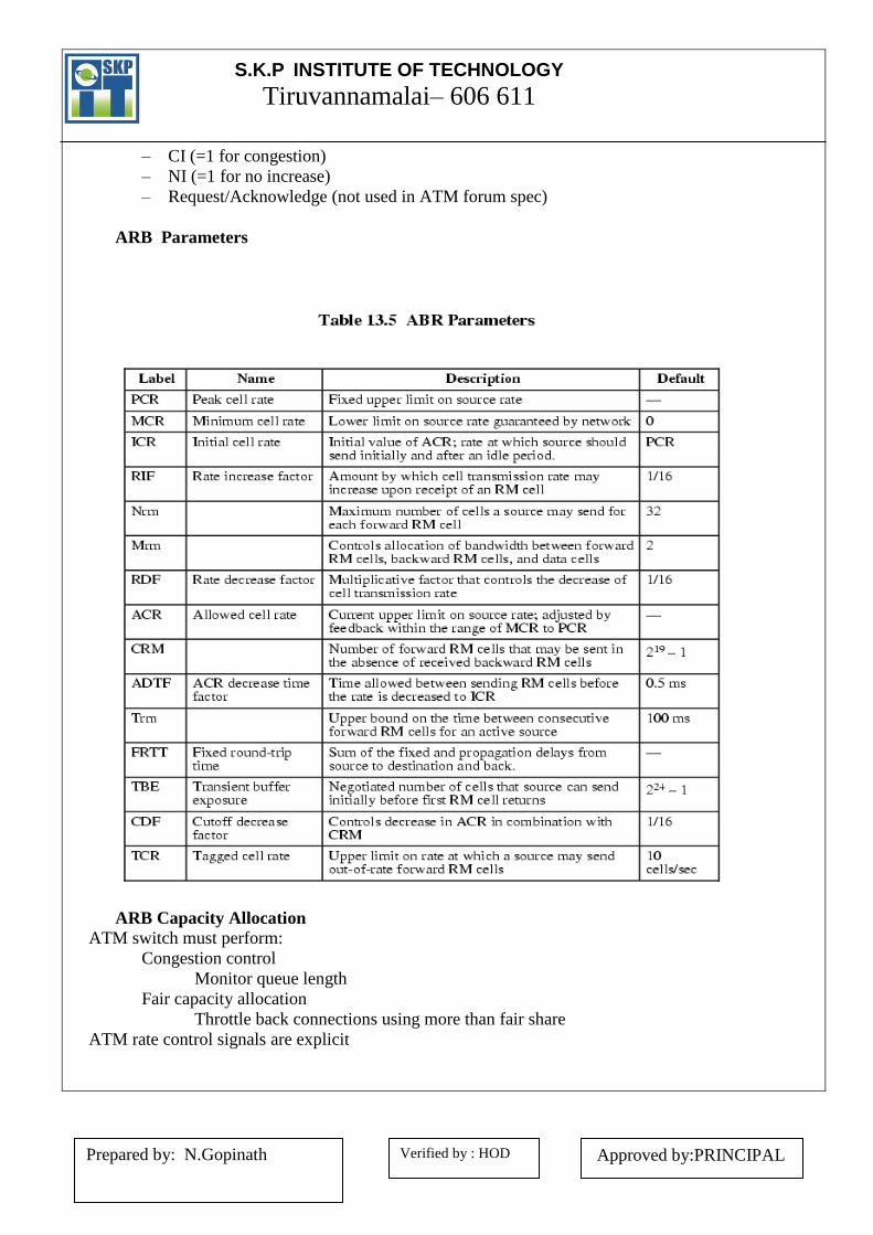
S.K.P INSTITUTE OF TECHNOLOGY Tiruvannamalai– 606 611
Verified by : HOD Prepared by: N.Gopinath
Approved by:PRINCIPAL
– CI (=1 for congestion)
– NI (=1 for no increase)
– Request/Acknowledge (not used in ATM forum spec)
ARB Parameters
ARB Capacity Allocation
ATM switch must perform:
Congestion control
Monitor queue length
Fair capacity allocation
Throttle back connections using more than fair share
ATM rate control signals are explicit

S.K.P INSTITUTE OF TECHNOLOGY Tiruvannamalai– 606 611
Verified by : HOD Prepared by: N.Gopinath
Approved by:PRINCIPAL
TCP are implicit
Increasing delay and cell loss
Congestion Control Algorithms-Binary Feedback
Use only EFCI, CI and NI bits
Switch monitors buffer utilization
When congestion approaches, binary notification
– Set EFCI on forward data cells or CI or NI on FRM or BRM
Three approaches to which to notify
– Single FIFO queue
– Multiple queues
– Fair share notification
Single FIFO Queue
When buffer use exceeds threshold (e.g. 80%)
– Switch starts issuing binary notifications
– Continues until buffer use falls below threshold
– Can have two thresholds
One for start and one for stop
Stops continuous on/off switching
– Biased against connections passing through more switches
Multiple Queues
Separate queue for each VC or group of VCs
Separate threshold on each queue
Only connections with long queues get binary notifications
– Fair
– Badly behaved source does not affect other VCs
– Delay and loss behaviour of individual VCs separated
Can have different QoS on different VCs
Fair Share
Selective feedback or intelligent marking
Try to allocate capacity dynamically
E.g.
fairshare =(target rate)/(number of connections)
Mark any cells where CCR>fairshare
Explicit Rate Feedback Schemes
Compute fair share of capacity for each VC
Determine current load or congestion
Compute explicit rate (ER) for each connection and send to source
Three algorithms
– Enhanced proportional rate control algorithm
EPRCA
– Explicit rate indication for congestion avoidance
ERICA

S.K.P INSTITUTE OF TECHNOLOGY Tiruvannamalai– 606 611
Verified by : HOD Prepared by: N.Gopinath
Approved by:PRINCIPAL
– Congestion avoidance using proportional control
CAPC
Enhanced Proportional Rate Control Algorithm(EPRCA
Switch tracks average value of current load on each connection
– Mean allowed cell rate (MARC)
– MACR(I)=(1-α)*(MACR(I-1) + α*CCR(I)
– CCR(I) is CCR field in Ith FRM
– Typically α=1/16
– Bias to past values of CCR over current
– Gives estimated average load passing through switch
– If congestion, switch reduces each VC to no more than DPF*MACR
DPF=down pressure factor, typically 7/8
ER<-min[ER, DPF*MACR]
Load Factor
Adjustments based on load factor
LF=Input rate/target rate
– Input rate measured over fixed averaging interval
– Target rate slightly below link bandwidth (85 to 90%)
– LF>1 congestion threatened
VCs will have to reduce rate
Explicit Rate Indication for Congestion Avoidance (ERICA)
Attempt to keep LF close to 1
Define:
fairshare = (target rate)/(number of connections)
VCshare = CCR/LF
= (CCR/(Input Rate)) *(Target Rate)
ERICA selectively adjusts VC rates
– Total ER allocated to connections matches target rate
– Allocation is fair
– ER = max[fairshare, VCshare]
– VCs whose VCshare is less than their fairshare get greater increase
Congestion Avoidance Using Proportional Control (CAPC)
If LF<1 fairshare<-fairshare*min[ERU,1+(1-LF)*Rup]
If LF>1 fairshare<-fairshare*min[ERU,1-(1-LF)*Rdn]
ERU>1, determines max increase
Rup between 0.025 and 0.1, slope parameter
Rdn, between 0.2 and 0.8, slope parameter
ERF typically 0.5, max decrease in allottment of fair share
If fairshare < ER value in RM cells, ER<-fairshare
Simpler than ERICA
Can show large rate oscillations if RIF (Rate increase factor) too high
Can lead to unfairness
GRF Overview
Simple as UBR from end system view

S.K.P INSTITUTE OF TECHNOLOGY Tiruvannamalai– 606 611
Verified by : HOD Prepared by: N.Gopinath
Approved by:PRINCIPAL
– End system does no policing or traffic shaping
– May transmit at line rate of ATM adaptor
Modest requirements on ATM network
No guarantee of frame delivery
Higher layer (e.g. TCP) react to congestion causing dropped frames
User can reserve cell rate capacity for each VC
– Application can send at min rate without loss
Network must recognise frames as well as cells
If congested, network discards entire frame
All cells of a frame have same CLP setting
– CLP=0 guaranteed delivery, CLP=1 best efforts
GFR Traffic Contract
Peak cell rate PCR
Minimum cell rate MCR
Maximum burst size MBS
Maximum frame size MFS
Cell delay variation tolerance CDVT
Mechanisms for supporting Rate Guarantees
Tagging and policing
Buffer management
Scheduling
Tagging and Policing
Tagging identifies frames that conform to contract and those that don’t
– CLP=1 for those that don’t
Set by network element doing conformance check
May be network element or source showing less important frames
– Get lower QoS in buffer management and scheduling
– Tagged cells can be discarded at ingress to ATM network or subsequent switch
– Discarding is a policing function
Buffer Management
Treatment of cells in buffers or when arriving and requiring buffering
If congested (high buffer occupancy) tagged cells discarded in preference to untagged
Discard tagged cell to make room for untagged cell
May buffer per-VC
Discards may be based on per queue thresholds
Scheduling
Give preferential treatment to untagged cells
Separate queues for each VC
– Per VC scheduling decisions
– E.g. FIFO modified to give CLP=0 cells higher priority
Scheduling between queues controls outgoing rate of VCs
– Individual cells get fair allocation while meeting traffic contract

S.K.P INSTITUTE OF TECHNOLOGY Tiruvannamalai– 606 611
Verified by : HOD Prepared by: N.Gopinath
Approved by:PRINCIPAL
Components of GFR Mechanism
GFR Conformance Definition
UPC function
– UPC monitors VC for traffic conformance
– Tag or discard non-conforming cells
Frame conforms if all cells in frame conform
– Rate of cells within contract
Generic cell rate algorithm PCR and CDVT specified for connection
– All cells have same CLP
– Within maximum frame size (MFS)
QoS Eligibility Test
Test for contract conformance
– Discard or tag non-conforming cells
Looking at upper bound on traffic
– Determine frames eligible for QoS guarantee
Under GFR contract for VC
Looking at lower bound for traffic
Frames are one of:
– Nonconforming: cells tagged or discarded
– Conforming ineligible: best efforts
– Conforming eligible: guaranteed delivery
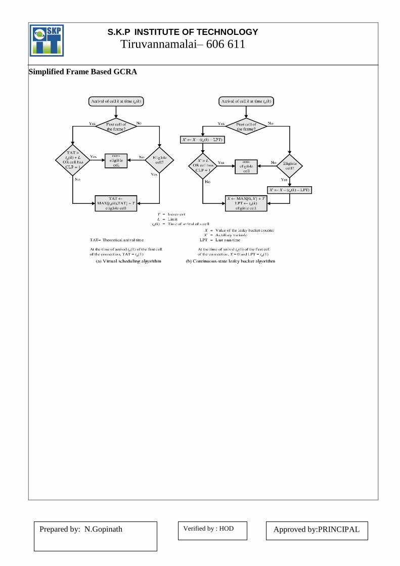
S.K.P INSTITUTE OF TECHNOLOGY Tiruvannamalai– 606 611
Verified by : HOD Prepared by: N.Gopinath
Approved by:PRINCIPAL
Simplified Frame Based GCRA

S.K.P INSTITUTE OF TECHNOLOGY Tiruvannamalai– 606 611
Verified by : HOD Prepared by: N.Gopinath
Approved by:PRINCIPAL
Unit IV
Integrated and Differentiated Services Introduction
New additions to Internet increasing traffic
–High volume client/server application
–Web
Graphics
–Real time voice and video
Need to manage traffic and control congestion
IEFT standards
–Integrated services
Collective service to set of traffic demands in domain
–Limit demand & reserve resources
–Differentiated services
Classify traffic in groups
Different group traffic handled differently
Integrated Services Architecture (ISA) IPv4 header fields for precedence and type of service usually ignored
ATM only network designed to support TCP, UDP and real-time traffic
–May need new installation
Need to support Quality of Service (QoS) within TCP/IP
–Add functionality to routers
–Means of requesting QoS
Internet Traffic – Elastic Can adjust to changes in delay and throughput
E.g. common TCP and UDP application
–E-Mail – insensitive to delay changes
–FTP – User expect delay proportional to file size
Sensitive to changes in throughput
–SNMP – delay not a problem, except when caused by congestion
–Web (HTTP), TELNET – sensitive to delay
Not per packet delay – total elapsed time
–E.g. web page loading time
–For small items, delay across internet dominates
–For large items it is throughput over connection
Need some QoS control to match to demand
Internet Traffic – Inelastic
Does not easily adapt to changes in delay and throughput
–Real time traffic
Throughput
–Minimum may be required
Delay
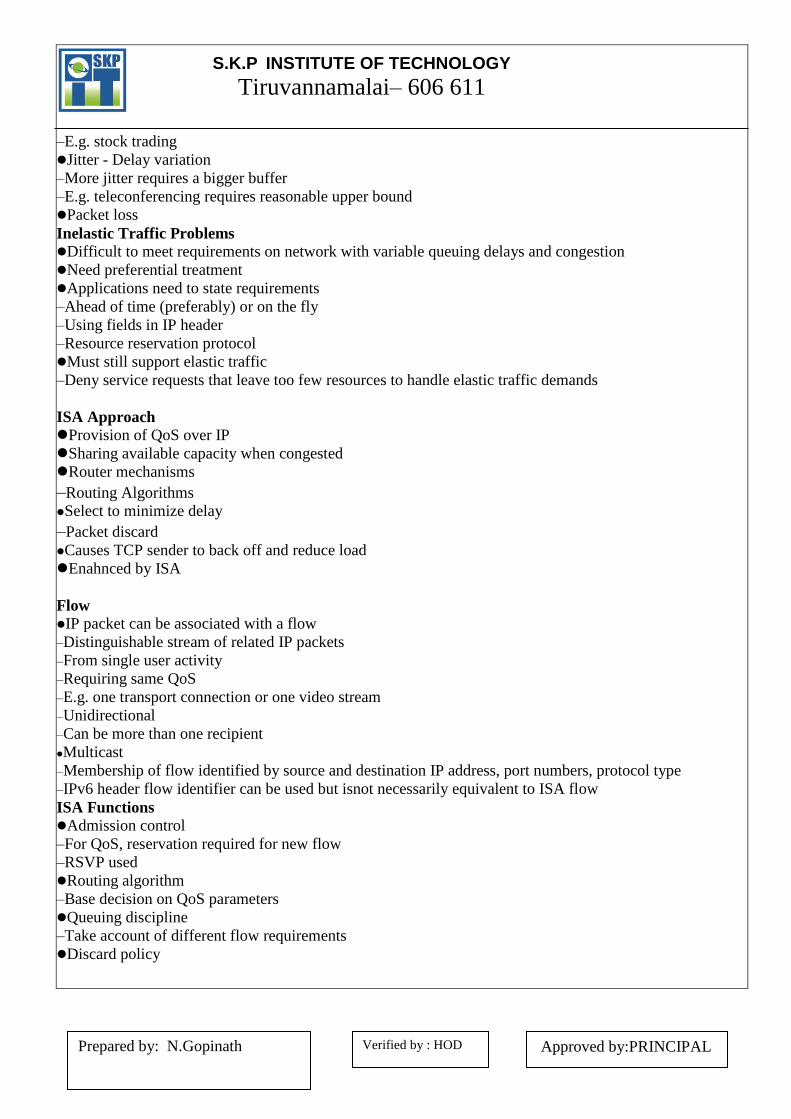
S.K.P INSTITUTE OF TECHNOLOGY Tiruvannamalai– 606 611
Verified by : HOD Prepared by: N.Gopinath
Approved by:PRINCIPAL
–E.g. stock trading
Jitter - Delay variation
–More jitter requires a bigger buffer
–E.g. teleconferencing requires reasonable upper bound
Packet loss
Inelastic Traffic Problems
Difficult to meet requirements on network with variable queuing delays and congestion
Need preferential treatment
Applications need to state requirements
–Ahead of time (preferably) or on the fly
–Using fields in IP header
–Resource reservation protocol
Must still support elastic traffic
–Deny service requests that leave too few resources to handle elastic traffic demands
ISA Approach
Provision of QoS over IP
Sharing available capacity when congested
Router mechanisms
–Routing Algorithms
Select to minimize delay
–Packet discard
Causes TCP sender to back off and reduce load
Enahnced by ISA
Flow
IP packet can be associated with a flow
–Distinguishable stream of related IP packets
–From single user activity
–Requiring same QoS
–E.g. one transport connection or one video stream
–Unidirectional
–Can be more than one recipient
Multicast
–Membership of flow identified by source and destination IP address, port numbers, protocol type
–IPv6 header flow identifier can be used but isnot necessarily equivalent to ISA flow
ISA Functions
Admission control
–For QoS, reservation required for new flow
–RSVP used
Routing algorithm
–Base decision on QoS parameters
Queuing discipline
–Take account of different flow requirements
Discard policy

S.K.P INSTITUTE OF TECHNOLOGY Tiruvannamalai– 606 611
Verified by : HOD Prepared by: N.Gopinath
Approved by:PRINCIPAL
–Manage congestion
–Meet QoS
ISA Implementation in Router
Background Functions
Forwarding functions
ISA Components – Background Functions
Reservation Protocol
–RSVP
Admission control
Management agent
–Can use agent to modify traffic control database and direct admission control
Routing protocol
ISA Components – Forwarding
Classifier and route selection
–Incoming packets mapped to classes
Single flow or set of flows with same QoS
–E.g. all video flows
Based on IP header fields
–Determines next hop
Packet scheduler
–Manages one or more queues for each output
–Order queued packets sent
Based on class, traffic control database, current and past activity on outgoing port

S.K.P INSTITUTE OF TECHNOLOGY Tiruvannamalai– 606 611
Verified by : HOD Prepared by: N.Gopinath
Approved by:PRINCIPAL
–Policing
ISA Services
Traffic specification (TSpec) defined as service for flow
On two levels
–General categories of service
Guaranteed
Controlled load
Best effort (default)
–Particular flow within category
TSpec is part of contract
Token Bucket
Many traffic sources can be defined by token bucket scheme
Provides concise description of load imposed by flow
–Easy to determine resource requirements
Provides input parameters to policing function
Token Bucket Diagram
ISA Services –
Guaranteed Service
Assured capacity level or data rate
Specific upper bound on queuing delay through network
–Must be added to propagation delay or latency to get total delay
–Set high to accommodate rare long queue delays
No queuing losses
–I.e. no buffer overflow
E.g. Real time play back of incoming signal can use delay buffer for incoming signal but will not tolerate
packet loss

S.K.P INSTITUTE OF TECHNOLOGY Tiruvannamalai– 606 611
Verified by : HOD Prepared by: N.Gopinath
Approved by:PRINCIPAL
ISA Services –
Controlled Load
Tightly approximates to best efforts under unloaded conditions
No upper bound on queuing delay
–High percentage of packets do not experience delay over minimum transit delay
Propagation plus router processing with no queuing delay
Very high percentage delivered
–Almost no queuing loss
Adaptive real time applications
–Receiver measures jitter and sets playback point
–Video can drop a frame or delay output slightly
–Voice can adjust silence periods
Queuing Discipline
Traditionally first in first out (FIFO) or first come first served (FCFS) at each router port
No special treatment to high priority packets (flows)
Small packets held up by large packets ahead of them in queue
–Larger average delay for smaller packets
–Flows of larger packets get better service
Greedy TCP connection can crowd out altruistic connections
–If one connection does not back off, others may back off more
Fair Queuing (FQ)
Multiple queues for each port
–One for each source or flow
–Queues services round robin
–Each busy queue (flow) gets exactly one packet per cycle
–Load balancing among flows
–No advantage to being greedy
Your queue gets longer, increasing your delay
–Short packets penalized as each queue sends one packet per cycle
FIFO and FQ
Processor Sharing
Multiple queues as in FQ

S.K.P INSTITUTE OF TECHNOLOGY Tiruvannamalai– 606 611
Verified by : HOD Prepared by: N.Gopinath
Approved by:PRINCIPAL
Send one bit from each queue per round
–Longer packets no longer get an advantage
Can work out virtual (number of cycles) start and finish time for a given packet
However, we wish to send packets, not bits
Bit-Round Fair Queuing (BRFQ)
Compute virtual start and finish time as before
When a packet finished, the next packet sent is the one with the earliest virtual finish time
Good approximation to performance of PS
–Throughput and delay converge as time increases
Comparison of FIFO, FQ and BRFQ
Generalized Processor Sharing (GPS)
BRFQ can not provide different capacities to different flows
Enhancement called Weighted fair queue (WFQ)
From PS, allocate weighting to each flow that determines how many bots are sent during each round
–If weighted 5, then 5 bits are sent per round
Gives means of responding to different service requests
Guarantees that delays do not exceed bounds
Weighted Fair Queue
Emulates bit by bit GPS

S.K.P INSTITUTE OF TECHNOLOGY Tiruvannamalai– 606 611
Verified by : HOD Prepared by: N.Gopinath
Approved by:PRINCIPAL
Same strategy as BRFQ
FIFO v WFQ
\
Proactive Packet Discard
Congestion management by proactive packet discard
–Before buffer full
–Used on single FIFO queue or multiple queues for elastic traffic
–E.g. Random Early Detection (RED)
Random Early Detection (RED)
Motivation
Surges fill buffers and cause discards
On TCP this is a signal to enter slow start phase, reducing load
–Lost packets need to be resent
Adds to load and delay
–Global synchronization

S.K.P INSTITUTE OF TECHNOLOGY Tiruvannamalai– 606 611
Verified by : HOD Prepared by: N.Gopinath
Approved by:PRINCIPAL
Traffic burst fills queues so packets lost
Many TCP connections enter slow start
Traffic drops so network under utilized
Connections leave slow start at same time causing burst
Bigger buffers do not help
Try to anticipate onset of congestion and tell one connection to slow down
RED Design Goals Congestion avoidance
Global synchronization avoidance
–Current systems inform connections to back off implicitly by dropping packets
Avoidance of bias to bursty traffic
–Discard arriving packets will do this
Bound on average queue length
–Hence control on average delay
RED Algorithm – Overview
Calculate average queue size avg
if avg < THmin
queue packet
else if THmin avg Thmax
calculate probability Pa
with probability Pa
discard packet
else with probability 1-Pa
queue packet
else if avg THmax
discard packet
RED Buffer

S.K.P INSTITUTE OF TECHNOLOGY Tiruvannamalai– 606 611
Verified by : HOD Prepared by: N.Gopinath
Approved by:PRINCIPAL
RED Algorithm Detail

S.K.P INSTITUTE OF TECHNOLOGY Tiruvannamalai– 606 611
Verified by : HOD Prepared by: N.Gopinath
Approved by:PRINCIPAL
Differentiated Services (DS)
ISA and RSVP complex to deploy
May not scale well for large volumes of traffic
–Amount of control signals
–Maintenance of state information at routers
DS architecture designed to provide simple, easy to implement, low overhead tool
–Support range of network services
Differentiated on basis of performance
Characteristics of DS
Use IPv4 header Type of Service or IPv6 Traffic Class field
–No change to IP
Service level agreement (SLA) established between provider (internet domain) and customer prior to use
of DS
–DS mechanisms not needed in applications
Build in aggregation
–All traffic with same DS field treated same
E.g. multiple voice connections
–DS implemented in individual routers by queuing and forwarding based on DS field
State information on flows not saved by routers
Services Provided within DS domain
–Contiguous portion of Internet over which consistent set of DS policies administered
–Typically under control of one administrative entity
Defined in SLA
–Customer may be user organization or other DS domain
–Packet class marked in DS field
Service provider configures forwarding policies routers
–Ongoing measure of performance provided for each class
DS domain expected to provide agreed service internally
If destination in another domain, DS domain attempts to forward packets through other domains
–Appropriate service level requested from each domain
SLA Parameters
Detailed service performance parameters
–Throughput, drop probability, latency
Constraints on ingress and egress points
–Indicate scope of service
Traffic profiles to be adhered to
–Token bucket
Disposition of traffic in excess of profile
Example Services
Qualitative

S.K.P INSTITUTE OF TECHNOLOGY Tiruvannamalai– 606 611
Verified by : HOD Prepared by: N.Gopinath
Approved by:PRINCIPAL
–A: Low latency
–B: Low loss
Quantitative
–C: 90% in-profile traffic delivered with no more than 50ms latency
–D: 95% in-profile traffic delivered
Mixed
–E: Twice bandwidth of F
–F: Traffic with drop precedence X has higher delivery probability than that with drop precedence Y
DS Field Detail
Leftmost 6 bits are DS codepoint
–64 different classes available
–3 pools
xxxxx0 : reserved for standards
–000000 : default packet class
–xxx000 : reserved for backwards compatibility with IPv4 TOS
xxxx11 : reserved for experimental or local use
xxxx01 : reserved for experimental or local use but may be allocated for future standards if needed
Rightmost 2 bits unused
Configuration Diagram
Configuration – Interior Routers
Domain consists of set of contiguous routers
Interpretation of DS codepoints within domain is consistent
Interior nodes (routers) have simple mechanisms to handle packets based on codepoints
–Queuing gives preferential treatment depending on codepoint
Per Hop behaviour (PHB)
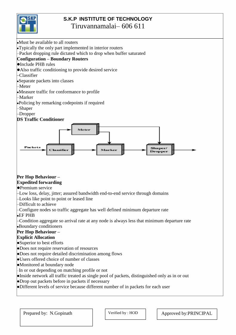
S.K.P INSTITUTE OF TECHNOLOGY Tiruvannamalai– 606 611
Verified by : HOD Prepared by: N.Gopinath
Approved by:PRINCIPAL
Must be available to all routers
Typically the only part implemented in interior routers
–Packet dropping rule dictated which to drop when buffer saturated
Configuration – Boundary Routers
Include PHB rules
Also traffic conditioning to provide desired service
–Classifier
Separate packets into classes
–Meter
Measure traffic for conformance to profile
–Marker
Policing by remarking codepoints if required
–Shaper
–Dropper
DS Traffic Conditioner
Per Hop Behaviour –
Expedited forwarding
Premium service
–Low loss, delay, jitter; assured bandwidth end-to-end service through domains
–Looks like point to point or leased line
–Difficult to achieve
–Configure nodes so traffic aggregate has well defined minimum departure rate
EF PHB
–Condition aggregate so arrival rate at any node is always less that minimum departure rate
Boundary conditioners
Per Hop Behaviour –
Explicit Allocation
Superior to best efforts
Does not require reservation of resources
Does not require detailed discrimination among flows
Users offered choice of number of classes
Monitored at boundary node
–In or out depending on matching profile or not
Inside network all traffic treated as single pool of packets, distinguished only as in or out
Drop out packets before in packets if necessary
Different levels of service because different number of in packets for each user

S.K.P INSTITUTE OF TECHNOLOGY Tiruvannamalai– 606 611
Verified by : HOD Prepared by: N.Gopinath
Approved by:PRINCIPAL
PHB - Assured Forwarding
Four classes defined
–Select one or more to meet requirements
Within class, packets marked by customer or provider with one of three drop precedence values
–Used to determine importance when dropping packets as result of congestion
Codepoints for AF PHB

S.K.P INSTITUTE OF TECHNOLOGY Tiruvannamalai– 606 611
Verified by : HOD Prepared by: N.Gopinath
Approved by:PRINCIPAL
Unit V
Protocols for QoS Support Increased Demands
Need to incorporate bursty and stream traffic in TCP/IP architecture
Increase capacity
– Faster links, switches, routers
– Intelligent routing policies
– End-to-end flow control
Multicasting
Quality of Service (QoS) capability
Transport protocol for streaming
Resource Reservation - Unicast
Prevention as well as reaction to congestion required
Can do this by resource reservation
Unicast
– End users agree on QoS for task and request from network
– May reserve resources
– Routers pre-allocate resources
– If QoS not available, may wait or try at reduced QoS
Resource Reservation – Multicast
Generate vast traffic
– High volume application like video
– Lots of destinations
Can reduce load
– Some members of group may not want current transmission
“Channels” of video
– Some members may only be able to handle part of transmission
Basic and enhanced video components of video stream
Routers can decide if they can meet demand
Resource Reservation Problems on an Internet
Must interact with dynamic routing
– Reservations must follow changes in route
Soft state – a set of state information at a router that expires unless refreshed
– End users periodically renew resource requests
Resource ReSerVation Protocol (RSVP) Design Goals
Enable receivers to make reservations
– Different reservations among members of same multicast group allowed
Deal gracefully with changes in group membership
– Dynamic reservations, separate for each member of group
Aggregate for group should reflect resources needed
– Take into account common path to different members of group
Receivers can select one of multiple sources (channel selection)
Deal gracefully with changes in routes

S.K.P INSTITUTE OF TECHNOLOGY Tiruvannamalai– 606 611
Verified by : HOD Prepared by: N.Gopinath
Approved by:PRINCIPAL
– Re-establish reservations
Control protocol overheadIndependent of routing protocol
RSVP Characteristics
Unicast and Multicast
Simplex
– Unidirectional data flow
– Separate reservations in two directions
Receiver initiated
– Receiver knows which subset of source transmissions it wants
Maintain soft state in internet
– Responsibility of end users
Providing different reservation styles
– Users specify how reservations for groups are aggregated
Transparent operation through non-RSVP routers
Support IPv4 (ToS field) and IPv6 (Flow label field)
Data Flows - Session
Data flow identified by destination
Resources allocated by router for duration of session
Defined by
– Destination IP address
Unicast or multicast
– IP protocol identifier
TCP, UDP etc.
– Destination port
May not be used in multicast
Flow Descriptor
Reservation Request
– Flow spec
Desired QoS
Used to set parameters in node’s packet scheduler
Service class, Rspec (reserve), Tspec (traffic)
– Filter spec
Set of packets for this reservation
Source address, source prot
Treatment of Packets of One Session at One Router

S.K.P INSTITUTE OF TECHNOLOGY Tiruvannamalai– 606 611
Verified by : HOD Prepared by: N.Gopinath
Approved by:PRINCIPAL
RSVP Operation Diagram
RSVP Operation
G1, G2, G3 members of multicast group
S1, S2 sources transmitting to that group
Heavy black line is routing tree for S1, heavy grey line for S2
Arrowed lines are packet transmission from S1 (black) and S2 (grey)
All four routers need to know reservation s for each multicast address

S.K.P INSTITUTE OF TECHNOLOGY Tiruvannamalai– 606 611
Verified by : HOD Prepared by: N.Gopinath
Approved by:PRINCIPAL
– Resource requests must propagate back through routing tree
Filtering
G3 has reservation filter spec including S1 and S2
G1, G2 from S1 only
R3 delivers from S2 to G3 but does not forward to R4
G1, G2 send RSVP request with filter excluding S2
G1, G2 only members of group reached through R4
– R4 doesn’t need to forward packets from this session
– R4 merges filter spec requests and sends to R3
R3 no longer forwards this session’s packets to R4
– Handling of filtered packets not specified
– Here they are dropped but could be best efforts delivery
R3 needs to forward to G3
– Stores filter spec but doesn’t propagate it
Reservation Styles Determines manner in which resource requirements from members of group are aggregated
Reservation attribute
– Reservation shared among senders (shared)
Characterizing entire flow received on multicast address
– Allocated to each sender (distinct)
Simultaneously capable of receiving data flow from each sender
Sender selection
– List of sources (explicit)
– All sources, no filter spec (wild card)
Reservation Attributes and Styles Reservation Attribute
– Distinct
Sender selection explicit = Fixed filter (FF)
Sender selection wild card = none
– Shared
Sender selection explicit= Shared-explicit (SE)
Sender selection wild card = Wild card filter (WF)
Wild Card Filter Style
Single resource reservation shared by all senders to this address
If used by all receivers: shared pipe whose capacity is largest of resource requests from receivers
downstream from any point on tree
Independent of number of senders using it
Propagated upstream to all senders
WF(*{Q})

S.K.P INSTITUTE OF TECHNOLOGY Tiruvannamalai– 606 611
Verified by : HOD Prepared by: N.Gopinath
Approved by:PRINCIPAL
– * = wild card sender
– Q = flowspec
Audio teleconferencing with multiple sites
Fixed Filter Style Distinct reservation for each sender
Explicit list of senders
FF(S1{Q!}, S2{Q2},…)
Video distribution
Shared Explicit Style Single reservation shared among specific list of senders
SE(S1, S2, S3, …{Q})
Multicast applications with multiple data sources but unlikely to transmit simultaneously
RSVP Protocol Mechanisms Two message types
– Resv
Originate at multicast group receivers
Propagate upstream
Merged and packet when appropriate
Create soft states
Reach sender
– Allow host to set up traffic control for first hop
– Path
Provide upstream routing information
Issued by sending hosts
Transmitted through distribution tree to all destinations
RSVP Host Model
S.K.P INSTITUTE OF TECHNOLOGY Tiruvannamalai– 606 611
Verified by : HOD Prepared by: N.Gopinath
Approved by:PRINCIPAL
Summary
RSVP is a transport layer protocol that enables a network to provide differentiated levels of service to
specific flows of data. Ostensibly, different application types have different performance requirements.
RSVP acknowledges these differences and provides the mechanisms necessary to detect the levels of
performance required by different appli-cations and to modify network behaviors to accommodate those
required levels. Over time, as time and latency-sensitive applications mature and proliferate, RSVP's
capabilities will become increasingly important.
Review Questions
Q—Is it necessary to migrate away from your existing routing protocol to support RSVP?
A—RSVP is not a routing protocol. Instead, it was designed to work in conjunction with existing routing
protocols. Thus, it is not necessary to migrate to a new routing protocol to support RSVP.
Q—Identify the three RSVP levels of service, and explain the difference among them.
A—RSVP's three levels of service include best-effort, rate-sensitive, and delay-sensitive service. Best-
effort service is used for applications that require reliable delivery rather than a timely delivery. Rate-
sensitive service is used for any traffic that is sensitive to variation in the amount of bandwidth available.
Such applications include H.323 videoconferencing, which was designed to run at a nearly constant rate.
RSVP's third level of service is delay-sensitive service. Delay-sensitive traffic requires timely but not
reliable delivery of data.
Q—What are the two RSVP reservation classes, and how do they differ?
A—A reservation style is a set of control options that defines how a reservation operates. RSVP supports
two primary types of reservation styles: distinct reservations and shared reservations. A distinct reservation
establishes a flow for each sending device in a session. Shared reservations aggregate communications
flows for a set of senders. Each of these two reservation styles is defined by a series of filters.
Q—What are RSVP filters?
A—A filter in RSVP is a specific set of control options that specifies operational parameters for a
reservation. RSVP's styles include wildcard-filter (WF), fixed-filter (FF), and shared-explicit (SE) filters.
Q—How can RSVP be used through network regions that do not support RSVP?
A—RSVP supports tunneling through network regions that do not support RSVP. This capability was
developed to enable a phased-in implementation of RSVP.
Multiprotocol Label Switching (MPLS) Routing algorithms provide support for performance goals

S.K.P INSTITUTE OF TECHNOLOGY Tiruvannamalai– 606 611
Verified by : HOD Prepared by: N.Gopinath
Approved by:PRINCIPAL
– Distributed and dynamic
React to congestion
Load balance across network
– Based on metrics
Develop information that can be used in handling different service needs
Enhancements provide direct support
– IS, DS, RSVP
Nothing directly improves throughput or delay
MPLS tries to match ATM QoS support
Background Efforts to marry IP and ATM
IP switching (Ipsilon)
Tag switching (Cisco)
Aggregate route based IP switching (IBM)
Cascade (IP navigator)
All use standard routing protocols to define paths between end points
Assign packets to path as they enter network
Use ATM switches to move packets along paths
– ATM switching (was) much faster than IP routers
– Use faster technology
Developments IETF working group in 1997, proposed standard 2001
Routers developed to be as fast as ATM switches
– Remove the need to provide both technologies in same network
MPLS does provide new capabilities
– QoS support
– Traffic engineering
– Virtual private networks
– Multiprotocol support
Connection Oriented QoS Support
Guarantee fixed capacity for specific applications
Control latency/jitter
Ensure capacity for voice
Provide specific, guaranteed quantifiable SLAs
Configure varying degrees of QoS for multiple customers
MPLS imposes connection oriented framework on IP based internets
Traffic Engineering
Ability to dynamically define routes, plan resource commitments based on known demands and
optimize network utilization
Basic IP allows primitive traffic engineering
– E.g. dynamic routing

S.K.P INSTITUTE OF TECHNOLOGY Tiruvannamalai– 606 611
Verified by : HOD Prepared by: N.Gopinath
Approved by:PRINCIPAL
MPLS makes network resource commitment easy
– Able to balance load in face of demand
– Able to commit to different levels of support to meet user traffic requirements
– Aware of traffic flows with QoS requirements and predicted demand
– Intelligent re-routing when congested
VPN Support
Traffic from a given enterprise or group passes transparently through an internet
Segregated from other traffic on internet
Performance guarantees
Security
Multiprotocol Support
MPLS can be used on different network technologies
IP
– Requires router upgrades
Coexist with ordinary routers
ATM
– Enables and ordinary switches co-exist
Frame relay
– Enables and ordinary switches co-exist
Mixed network
MPLS Terminology
MPLS Operation
Label switched routers capable of switching and routing packets based on label appended to packet
Labels define a flow of packets between end points or multicast destinations
Each distinct flow (forward equivalence class – FEC) has specific path through LSRs defined
– Connection oriented
Each FEC has QoS requirements
IP header not examined
– Forward based on label value

S.K.P INSTITUTE OF TECHNOLOGY Tiruvannamalai– 606 611
Verified by : HOD Prepared by: N.Gopinath
Approved by:PRINCIPAL
MPLS Operation Diagram
Explanation – Setup
Labelled switched path established prior to routing and delivery of packets
QoS parameters established along path
– Resource commitment
– Queuing and discard policy at LSR
– Interior routing protocol e.g. OSPF used
– Labels assigned
Local significance only
Manually or using Label distribution protocol (LDP) or enhanced version of RSVP
Explanation – Packet Handling
Packet enters domain through edge LSR
– Processed to determine QoS
LSR assigns packet to FEC and hence LSP
– May need co-operation to set up new LSP
Append label
Forward packet
Within domain LSR receives packet
Remove incoming label, attach outgoing label and forward
Egress edge strips label, reads IP header and forwards
Notes
MPLS domain is contiguous set of MPLS enabled routers
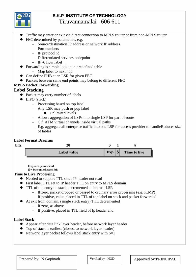
S.K.P INSTITUTE OF TECHNOLOGY Tiruvannamalai– 606 611
Verified by : HOD Prepared by: N.Gopinath
Approved by:PRINCIPAL
Traffic may enter or exit via direct connection to MPLS router or from non-MPLS router
FEC determined by parameters, e.g.
– Source/destination IP address or network IP address
– Port numbers
– IP protocol id
– Differentiated services codepoint
– IPv6 flow label
Forwarding is simple lookup in predefined table
– Map label to next hop
Can define PHB at an LSR for given FEC
Packets between same end points may belong to different FEC
MPLS Packet Forwarding
Label Stacking Packet may carry number of labels
LIFO (stack)
– Processing based on top label
– Any LSR may push or pop label
Unlimited levels
– Allows aggregation of LSPs into single LSP for part of route
– C.f. ATM virtual channels inside virtual paths
– E.g. aggregate all enterprise traffic into one LSP for access provider to handleReduces size
of tables
Label Format Diagram
Time to Live Processing
Needed to support TTL since IP header not read
First label TTL set to IP header TTL on entry to MPLS domain
TTL of top entry on stack decremented at internal LSR
– If zero, packet dropped or passed to ordinary error processing (e.g. ICMP)
– If positive, value placed in TTL of top label on stack and packet forwarded
At exit from domain, (single stack entry) TTL decremented
– If zero, as above
– If positive, placed in TTL field of Ip header and
Label Stack
Appear after data link layer header, before network layer header
Top of stack is earliest (closest to network layer header)
Network layer packet follows label stack entry with S=1

S.K.P INSTITUTE OF TECHNOLOGY Tiruvannamalai– 606 611
Verified by : HOD Prepared by: N.Gopinath
Approved by:PRINCIPAL
Over connection oriented services
– Topmost label value in ATM header VPI/VCI field
Facilitates ATM switching
– Top label inserted between cell header and IP header
– In DLCI field of Frame Relay
– Note: TTL problem
Position of MPLS Label Stack
FECs, LSPs, and Labels
Traffic grouped into FECs
Traffic in a FEC transits an MLPS domain along an LSP
Packets identified by locally significant label
At each LSR, labelled packets forwarded on basis of label.
– LSR replaces incoming label with outgoing label
Each flow must be assigned to a FEC
Routing protocol must determine topology and current conditions so LSP can be assigned to FEC
– Must be able to gather and use information to support QoS
LSRs must be aware of LSP for given FEC, assign incoming label to LSP, communicate label to
other LSRs
Topology of LSPs
Unique ingress and egress LSR
– Single path through domain
Unique egress, multiple ingress LSRs
– Multiple paths, possibly sharing final few hops
Multiple egress LSRs for unicast traffic
Multicast

S.K.P INSTITUTE OF TECHNOLOGY Tiruvannamalai– 606 611
Verified by : HOD Prepared by: N.Gopinath
Approved by:PRINCIPAL
Route Selection
Selection of LSP for particular FEC
Hop-by-hop
– LSR independently chooses next hop
– Ordinary routing protocols e.g. OSPF
– Doesn’t support traffic engineering or policy routing
Explicit
– LSR (usually ingress or egress) specifies some or all LSRs in LSP for given FEC
– Selected by configuration,or dynamically
Constraint Based Routing Algorithm
Take in to account traffic requirements of flows and resources available along hops
– Current utilization, existing capacity, committed services
– Additional metrics over and above traditional routing protocols (OSPF)
Max link data rate
Current capacity reservation
Packet loss ratio
Link propagation delay
Label Distribution
Setting up LSP
Assign label to LSP
Inform all potential upstream nodes of label assigned by LSR to FEC
– Allows proper packet labelling
– Learn next hop for LSP and label that downstream node has assigned to FEC
Allow LSR to map incoming to outgoing label
Real Time Transport Protocol
TCP not suited to real time distributed application
– Point to point so not suitable for multicast
– Retransmitted segments arrive out of order
– No way to associate timing with segments
UDP does not include timing information nor any support for real time applications
Solution is real-time transport protocol RTP
RTP Architecture
Close coupling between protocol and application layer functionality
– Framework for application to implement single protocol
Application level framing
Integrated layer processing
Application Level Framing
Recovery of lost data done by application rather than transport layer
– Application may accept less than perfect delivery
Real time audio and video

S.K.P INSTITUTE OF TECHNOLOGY Tiruvannamalai– 606 611
Verified by : HOD Prepared by: N.Gopinath
Approved by:PRINCIPAL
Inform source about quality of delivery rather than retransmit
Source can switch to lower quality
– Application may provide data for retransmission
Sending application may recompute lost values rather than storing them
Sending application can provide revised values
Can send new data to “fix” consequences of loss
Lower layers deal with data in units provided by application
– Application data units (ADU)
Integrated Layer Processing
Adjacent layers in protocol stack tightly coupled
Allows out of order or parallel functions from different layers
RTP Architecture Diagram
RTP Data Transfer Protocol
Transport of real time data among number of participants in a session, defined by:
– RTP Port number
UDP destination port number if using UDP
– RTP Control Protocol (RTCP) port number
Destination port address used by all participants for RTCP transfer
– IP addresses
Multicast or set of unicast
Multicast Support
Each RTP data unit includes:
Source identifier
Timestamp
Payload format
Relays
Intermediate system acting as receiver and transmitter for given protocol layer
Mixers
– Receives streams of RTP packets from one or more sources
– Combines streams
– Forwards new stream

S.K.P INSTITUTE OF TECHNOLOGY Tiruvannamalai– 606 611
Verified by : HOD Prepared by: N.Gopinath
Approved by:PRINCIPAL
Translators
– Produce one or more outgoing RTP packets for each incoming packet
– E.g. convert video to lower quality
RTP Header
RTP Control Protocol (RTCP)
RTP is for user data
RTCP is multicast provision of feedback to sources and session participants
Uses same underlying transport protocol (usually UDP) and different port number
RTCP packet issued periodically by each participant to other session members
RTCP Functions
QoS and congestion control
Identification
Session size estimation and scaling
Session control
RTCP Transmission
Number of separate RTCP packets bundled in single UDP datagram
– Sender report
– Receiver report
– Source description
– Goodbye
– Application specific

S.K.P INSTITUTE OF TECHNOLOGY Tiruvannamalai– 606 611
Verified by : HOD Prepared by: N.Gopinath
Approved by:PRINCIPAL
RTCP Packet Formats
Packet Fields (All Packets)
Version (2 bit) currently version 2
Padding (1 bit) indicates padding bits at end of control information, with number of octets as last octet of
padding
Count (5 bit) of reception report blocks in SR or RR, or source items in SDES or BYE
Packet type (8 bit)
Length (16 bit) in 32 bit words minus 1
In addition Sender and receiver reports have:
–Synchronization Source Identifier
Packet Fields (Sender Report)
Sender Information Block
NTP timestamp: absolute wall clock time when report sent
RTP Timestamp: Relative time used to create timestamps in RTP packets
Sender’s packet count (for this session)
Sender’s octet count (for this session)
Packet Fields (Sender Report)
Reception Report Block
SSRC_n (32 bit) identifies source refered to by this report block
Fraction lost (8 bits) since previous SR or RR

S.K.P INSTITUTE OF TECHNOLOGY Tiruvannamalai– 606 611
Verified by : HOD Prepared by: N.Gopinath
Approved by:PRINCIPAL
Cumulative number of packets lost (24 bit) during this session
Extended highest sequence number received (32 bit)
–Least significant 16 bits is highest RTP data sequence number received from SSRC_n
–Most significant 16 bits is number of times sequence number has wrapped to zero
Interarrival jitter (32 bit)
Last SR timestamp (32 bit)
Delay since last SR (32 bit)
Receiver Report
Same as sender report except:
–Packet type field has different value
–No sender information block
Source Description Packet
Used by source to give more information
32 bit header followed by zero or more additional information chunks
E.g.:
0 END End of SDES list
1 CNAME Canonical name
2 NAME Real user name of source
3 EMAIL Email address
Goodbye (BYE)
Indicates one or more sources no linger active
–Confirms departure rather than failure of network
Application Defined Packet
Experimental use
For functions & features that are application specific