1

Supporting Information for:

Size and Elemental Distributions of Nano- to Micro-

Particulates in the Geochemically-stratified Great

Salt Lake

Ximena Diaz†,§, William P. Johnson†,*

* Corresponding author e-mail:

, Diego Fernandez†, David L. Naftz‡,†

†Department of Geology & Geophysics, University of Utah, 135 S 1460 E Salt Lake

City, UT 84112; ‡ U.S. Geological Survey, 2329 West Orton Circle, Salt Lake City, UT

84119

william.johnson@utah.edu; phone: (801)581-5033; fax: (801) 581-7065. § Current address: Department of Extractive Metallurgy, Escuela Politécnica Nacional, Quito – Ecuador.

2

Water samples. Water samples for total and dissolved major and trace element

analysis were collected in acid-rinsed polyethylene bottles from four stations (2267,

2565, 2767 and 3510, Figure 3 in the text) at the Great Salt Lake (GSL). At two stations

(2267 and 2767), samples were collected from two depths representing the shallow brine

layer. At the remaining two stations (2565 and 3510), samples were collected from three

or four depths representing the shallow and deep brine layers and the interface between

them (0.2, 3, 8, and 6.5 m, respectively).

Five samples (250 mL) were collected from each location using a peristaltic pump with

acid-rinsed C-flex tubing (Cole-Parmer's Masterflex, Vernon Hills, IL). Two of the five

samples were filtered (0.45 µm pore size, capsule-type filter). Four replicates (2 filtered

and 2 raw) were acidified (trace metals grade nitric acid, 2 mL, 7.7 N); one replicate was

kept unacidified (raw unacidified, RU). All five replicates were stored on ice until to be

transferred to a refrigerator. One each of the filtered-acidified and raw-acidified samples

were sent to a contract lab (Frontier Geoscience, Seattle, WA) for total Se analysis. The

other replicates were stored at 4oC. The acidified replicates (filter and raw) were analyzed

for major and trace elements (Al, As, Ba, Ca, Cd, Co, Cu, Fe, K, Li, Mg, Mn, Mo, Na,

Ni, Pb, S, Sb, Se, Ti, U, V, Zn) via collision cell inductively-coupled plasma mass

spectrometry (CC-ICP-MS) at the University of Utah. The raw unacidified replicate was

used for particulate fractionation analysis via asymmetric flow field flow fractionation

(AF4) coupled with the CC-ICP-MS at the University of Utah.

At the remaining two stations (2565 and 3510), samples were collected from three or

four depths representing the shallow and deep brine layers and the interface between

them (0.2, 3, 8, and 6.5 m, respectively).

3

Aqueous characteristics of shallow and deep brines included temperature,

conductivity, pH, oxidation-reduction potential (ORP), density, salinity and dissolved

oxygen (DO), were measured using a Hydrolab Troll 9000 (In-Situ Inc., Fort Collins,

CO). The major changes in water chemistry coincided with transition to the deep brine

layer, about 6.5 m depth below surface, where dissolved oxygen (DO), oxidation-

reduction potential (ORP) and pH decreased and conductivity increased (Figure 1 in the

text). Temperature profile (Figure 2 in the text) demonstrated that the deep brine layer is

insulated and showed lesser temperature variation relative to shallow brine layer,

resulting in the deep brine layer being cooler than the shallow brine during summer, and

warmer than the shallow brine in winter.

Average total concentrations for trace metals analyzed in 66 raw acidified (RA) and 66

filtered acidified (FA) samples showed trends with depth (0.2 m, 3.3 m, 6.5 m and 8.0 m)

that differed among the elements (Figure S1). The samples were taken from locations

spread across the south arm of the Great Salt Lake, and showed consistent values that

allowed their averaging despite significant spatial distances between samples as shown in

the error bars (Figure S1).

Al, Mn, Fe, Ni and Pb showed increased concentration in the deep brine layer (below

6.5 m and 8.0 m depths) relative to the shallow brine layer (Figure S1 top) for the RA

samples. In contrast, Co, Cu, As and Ba showed equivalent concentrations in the shallow

brine layer and the upper portion of the deep brine layer; whereas their concentrations

increased significantly (from 19 to 79%) at the bottom of the deep brine layer (about 8.0

m below the lake surface). Mo, Sb, U and Se showed similar concentrations at all depths

(Figure S1 top).

4

In the FA samples Al and Mn showed increased concentration in the deep brine layer

(below 6.5 m and 8.0 m depths) relative to the shallow brine layer (Figure S1 bottom),

whereas the majority of the elements showed similar concentrations at all depths, except

Ni, Cu and Pb that showed larger concentrations near surface. Fe and Co showed lower

concentrations in the intermediate depths (3.3 and 6.5 m) (Figure S1 bottom).

Fractionation. The dimensions of the asymmetric flow field-flow fractionation (AF4)

channel used were 27.3 cm in length, 224 µm in thickness and a channel volume of 0.71

mL, calculated according to Litzén (1993). The membrane used in the channel was a

10K Da regenerated cellulose. The Postnova AF4 equipment automatically controls the

different outflow rates (to the detector, the cross flow and to the slot pump). However, the

use of a 1kDa membrane produced outflow rates that could not be precisely controlled by

the equipment. Therefore we used a 10kDa membrane in the AF4 channel.

The AF4 was connected to three detectors (UV absorbance, fluorescence and CC-ICP-

MS) in serie, via a 0.25-mm i.d. peek tubing. Anoxic samples (samples from the deep

brine layer) were kept in the AF4-CC-ICP-MS under anoxic conditions by degassing the

carrier with nitrogen prior to use. Great Salt Lake water samples were filtered

immediately before to inject into the AF4-CC-ICP-MS system, using a 0.45 µm syringe

filter (Nalgene* Syringe Filters, surfactant-free cellulose acetate (SFCA)), for both

nanosize ranges (0.5 to 7.5 nm; and, 10 to 250 nm). The CC-ICP-MS removes

interferences during detection by the attenuation of polyatomic ions of same mass (but

different cross sectional area) as the analyte via counter-current flow of He or H2 gas

immediately upstream of the mass spectrometer. Separate runs using helium and

5

hydrogen gases in the collision cell (to reduce polyatomic interferences) were used with

each sample.

The AF4 was calibrated using standard nanoparticles. Colloidal gold and fluorescent

latex beads with known sizes (10, 98 and 200 nm) were used to determine the operation

conditions for the nanoparticles range between 10 to 250 nm (Table 1 in the text, Figure

S2). For nanoparticles separation in this size range, the AF4 was programmed to use

three different cross-flows during the elution to improve the particle separation and the

intensity of the UV signal. The calibration curve to convert the retention time in particle

size (hydrodynamic diameter) is shown in Figure S2. The calibration curve included the

injection, transition and elution times.

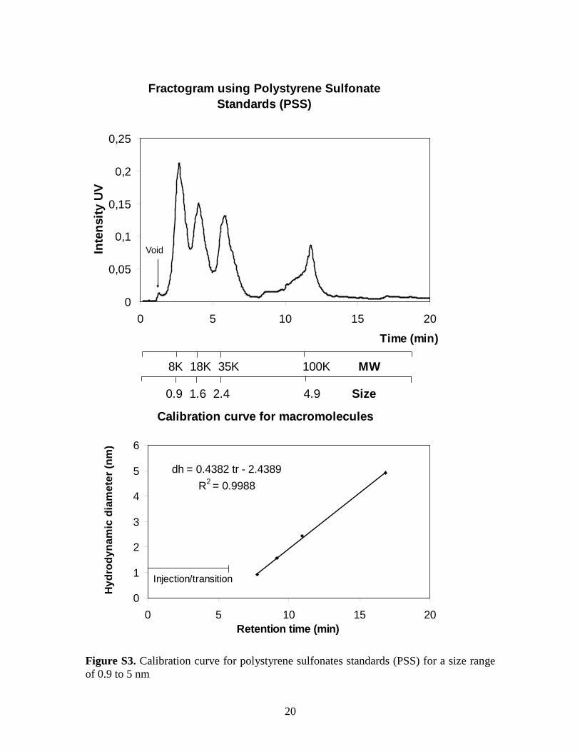
Polystyrene sulfonate standards (PSS) with known molecular weights (8K, 18K, 35K and

100K Da) were used to optimize the operation conditions to separate nanoparticles

between 0.9 to 7.5 nm in the AF4 (Table 2 in the text, Figure S3). A four-step program

varying the cross-flow in the AF4 was used during the elution, which improved the

particle separation and the intensity of the UV signal. To convert the retention time in

particle size the following expression derived from Prestel et al. (2005) was used:

log dh = 0.6685 log MW - 2.6517

where dh is the hydrodynamic diameter (in nm) and MW is the molecular weight (in Da).

The calibration curve obtained (Figure S3) included the injection, transition and elution

times and the variation of the cross flow during the run. The operation conditions for the

CC-ICP-MS are presented in Table S1.

Interestingly, the 8kDa standard showed a very strong signal even though the membrane

pore size was 10kDa. This may be due to a formation of an electric double layer on the

6

membrane (regenerated cellulose) that would be expected to extend 10s of nm into

solution, effectively decreasing the pore size of the membrane for PSS.

The AF4 fractionation may produce losses of standards due to the operation conditions

(e.g., high cross flow or cross flow changes during the run (Ratanathanawongs-Williams

& Giddings, 2000)); concentration of standards (e.g, overloading effects (Bolea et al.,

2006)); characteristics of membrane and analyte (e.g., absorption of the analyte to the

membrane (Bolea et al., 2006)). The material lost, that did not pass through the

membrane, may be eluted prior to the sample, or following cessation of cross flow if the

sample is held in place by cross flow. It has been suggested that the higher the cross flow

the higher the losses (Ratanathanawongs-Williams & Giddings, 2000). To account for

losses in a mixture of different-sized standards with variable cross flow is extremely

difficult (Ratanathanawongs-Williams & Giddings, 2000) and was not attempted in this

work.

The CC-ICP-MS removes interferences during detection by the attenuation of

polyatomic ions of same mass (but different cross sectional area) as the analyte via

counter-current flow of He or H2 gas immediately upstream of the mass spectrometer.

Separate runs using helium and hydrogen gases in the collision cell (to reduce polyatomic

interferences) were examined for each sample.

Fractionation of GSL synthetic and milli-Q water. A synthetic solution contained the

major salts (Cl-, Na+, Mg2+, SO42-, K+, Ca2+) that compose the shallow water of the GSL

(Table S2).

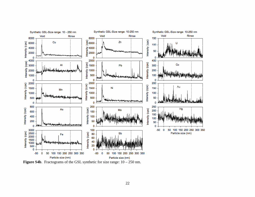
Results obtained in the GSL synthetic and in the milli-Q water fractionation for the 10

to 250 nm size range (Figure S4b) showed a void peak, which apparently seems to be an

7

AF4 artifact due to changes in pressure under the operational conditions used in this size

range. Not void peak was observed for the GSL synthetic or in the milli-Q water in the

0.9 to 7.5 nm size range (Figure S5b). Only one of the elements analyzed (Mn) in the

GSL synthetic solution showed a peak in the 0.9 – 7.5 nm size range similar to that

obtained in GSL water samples (Figure S5b), that could be due to contamination in the

salts used in the synthetic solution (Table S2).

PHREEQC Modeling of Water Samples. The U.S. Geological Survey (USGS)

PHREEQCI software (version 2.14.3, 2007,

://wwwbrr.cr.usgs.gov/projects/GWC_coupled/phreeqc/) was used to identify the

possible mineral phases present in raw acidified (RA) samples. Average concentrations

(Table S3) from multielement analysis of GSL water samples (RA) were used in the

modeling. The thermodynamic parameters used are defined in the minteq.v4 database,

which is an option incorporated to the program (Parkhurst and Appelo, 1999). The

minteq database has thermodynamic parameters for all major and trace metals analyzed

in this study. One important limitation of the PHREEQC is that the software uses Debye

Hückel expressions to account for the nonideality of aqueous solutions (Drever, 2002;

Appelo and Postman, 2005). Those expressions are suitable for low ionic strength but

may not be appropriate at higher ionic strengths (Drever, 2002) like for the hypersaline

water of the GSL. The latest version of the software has incorporated Pitzer activity

coefficients for major elements (e.g., Ba, Ca, Cl, Fe, K, Mg, Mn, Na, S) but not for trace

elements, which made ineffective for our purposes that database.

For the simulation, two extreme conditions of temperature observed in the shallow and

deep brine layers (2oC and 30oC for the shallow brine and 13oC and 20oC for the deep

8

brine) were used, to look for seasonal variability. Average values of densities measured

in the field (1.11 g/mL for the shallow brine and 1.16 g/mL for the deep brine) were

utilized. An average value of ORP (in mV) measured in the field were converted in pe

for each brine layer using the equation (Fengxiang and Banin, 1997):

pe = ORP(mV)/59.64

The pe values used for modeling were 3.4 for the shallow brine and -5 for the deep brine.

PHREEQC simulations were conducted to examine the mineralogical phases that were

supersaturated in both layers. These simulations are only approximate because the

PHRREQC software cannot correct the activity coefficients for the hypersaline

environment of the GSL.

In oxic brines PHREEQC predicted that the shallow brine is super-saturated with

silicates (clays), oxides and oxy-hydroxides of Fe and Al (Table S4 and Figure S6 top).

Elements such as Cu, Co and Mg were predicted to form complex compounds with Fe

oxide. Three U oxides were also predicted.

PHREEQC simulations for deep brine samples predicted that the majority of trace

metals precipitate as sulfides and selenides (Table S5 and Figure S6 bottom). The model

also predicted silicates (clays), Al oxy-hydroxides as well as uraninite (UO2) as stable

solid phases in the deep brine layer. Notably, there is one Fe-Al compound (FeAl2O4,

Hercynite) that was predicted for both brines (Tables S4, S5 and Figure S6).

The saturation indices (SI) were strongly dependent upon temperature, which ranges

from approximately 2oC to 30oC in the shallow brine layer of the Great Salt Lake (Table

S4).

9

SI decreased with increased temperature around 61% (average within a range from

28% to 96% among the compounds) for the Al oxy-hydroxides, such that Al

oxyhydroxides became undersaturated at the higher temperature. The opposite trend

occurred for the Fe oxy-hydroxides, which increased around 65% (average within a range

from 33% to 95% among the compounds) in response to increased temperature in the

observed range, showing that Fe oxy-hydroxides are more stable at higher temperature in

shallow brines.

The narrower temperature range in the deep brine, from approximately 13oC to 20oC,

yield a much reduced range in SI values in the deep brine relative to the shallow brine

layer. In general, the compounds predicted for the deep brine layer became less

supersaturated at higher temperature (Table S5).

Settling velocity in the water column of the Great Salt Lake. The approximate settling

velocity for equivalent spherical particles can be calculated by the Stoke’s equation as

follows:

Vs =ρs − ρ f( )gd 2

18µ

where Vs is the terminal velocity (in cm/s); ρs and ρf are the densities (in g/cm3) for the

solid and the fluid, respectively; g is the gravity constant (in cm/s2); µ is the viscosity (in

g/cm s); and, d is the particle diameter (in cm). For nanoparticles smaller than 100 nm,

electrostatic interactions and Brownian motion reduce the settling velocity virtually to

zero, especially for clays because of their aspect ratio. Stoke’s formula used here may

overestimate the settling velocity of nanoparticles larger than 100 nm, but was used for

10

comparison. Nanoparticles are commonly defined as particulate matter with at least one

dimension that is less than 100 nm (Christian et al. 2008).

A representative density is provided by boehmite (γ-AlOOH) nanoparticles (ρs = 3.04

g/cm3) for the range of nanoparticle sizes described here (0.5 to 450 nm). The time

required to settle 1 m in the shallow brine (ρf =1.1 g/cm3) ranges from 65 days (for a 450

nm nanoparticles) to 1.45*105 years (for a 0.5 nm nanoparticles) (Table S6); likewise in

the deep brine layer (ρf =1.16 g/cm3) the greater density will require larger time (Table

S6). For denser nanoparticles; e.g., pyrite (FeS2) (ρs = 5 g/cm3), the settling time in the

deep brine layer will require 33 days for 450 nm nanoparticles and 7.31*104 years for a

0.5 nm nanoparticle.

These results suggest that the downward transport between the layers may be one cause

to explain similarities in size distribution and elemental composition for the larger

particles (> 450 nm) between the two layers. However, for nanoparticle sizes < 50 nm

(> 14 years required to settle 1 m), downward transport cannot explain the similarities in

size distribution and elemental composition between the two layers. Furthermore, the

Great Salt Lake is rarely quiescent for periods of one, let alone two months of time.

Disturbance of the lake surface due to storms and wind events occurs frequently,

potentially mixing material between the two layers.

References

Appelo, C.A.J., and Postma, D. (2005) Geochemistry, groundwater and pollution. 2nd

Edition. A.A. Balkema Publishers, New York, pp. 123-132; 247-363; 436.

11

Bolea, E., Gorriz, M.P., Bouby, M., Laborda, F., Castillo, J.R., Geckeis, H. (2006)

Multielement characterization of metal-humic substances complexation by size exclusion

chromatography, asymmetrical flow field-flow fractionation, ultrafiltration and

inductively coupled plasma-mass spectrometry detection: A comparative approach.

Journal of Chromatography A, 1129, 236–246.

Christian, P., Von der Kammer, F., Baalousha, M., Hofmann, Th. (2008) Nanoparticles:

structure, properties, preparation and behaviour in environmental media. Ecotoxicology,

17, 326–343.

Drever, J.I. (2002) The Geochemistry of natural waters, surface and groundwater

environments, 3rd ed. reprinted; Prentice Hall: Upper Saddle River, pp. 26-33; 113-119,

185-196.

Fengxiang, H. and Banin, A. (1997) Long-term transformations and redistribution of

potentially toxic heavy metals in arid-zone soils incubated: I. Under saturated conditions.

Water, Air, & Soil Pollution 95, 399-423.

Litzén, A. (1993) Separation speed, retention, and dispersion in asymmetrical flow

field-flow fractionation as functions of channel dimensions and flow rates, Analytical

Chemistry, 65, 461-470.

Parkhurst, D.L. and Appelo, C.A.J. (1999) User's guide to PHREEQC (version 2) A

computer program for speciation, batch-reaction, one-dimensional transport, and inverse

geochemical calculations, USGS.

http://wwwbrr.cr.usgs.gov/projects/GWC_coupled/phreeqc/html/final.html

12

Prestel, H.; Schott, L.; Niessner, R.; Panne, U. (2005) Characterization of sewage plant

hydrocolloids using asymmetrical flow field-flow fractionation and ICP-mass

spectrometry. Water Res. 39, 3541-3552.

Ratanathanawongs-Williams, S.K. and Giddings, J.C. (2000) Sample recovery. IN

Field flow fractionation handbook. (eds. M.E. Schimpf, , K. Caldwell, and J.C.

Giddings), Wiley-Interscience, Inc., New York, pp. 325 - 343.

13

Tables and Figures

Table S1. CC-ICP-MS operation conditions. OPERATION CONDITIONS RF power (W) 1550 Plasma gas flowrate (L/min) 15 Hydrogen flowrate (mL/min) 2.5 Helium flowrate (mL/min) 2.5 Carrier flowrate (L/min) 0.8 Make-up gas (L/min) 0.2 Auxiliary gas (L/min) 0.9 Sample flowrate (mL/min) 0.3 Acquisition time per isotope (sec) 0.05 Repetition 3 Total acquisition time for 19 isotopes (sec) 2.85 Total running time (sec) 1500 - 1860 Tuning solution: 133Cs mean (cps) wth H2 in collision cell 34,000 % RSD < 3% Sample nebulizer tubing: Material Tygon Internal diameter (mm) 1.02 AF4 carrier tubing: Material Peek Internal diameter (mm) 0.25

Table S2. Great Salt Lake synthetic solution composition.

Salt

Concentration (mol/gsolution)

Concentration (g/L)

Grams in 100mL milli-Q water

Salt Purity Salt brand

NaCl 1.99E-03 116.7884 11.6788 99.999% Sigma-Aldrich

MgCl2 1.46E-04 13.9657 1.3966 99.99% Sigma

MgSO4 3.73E-05 4.4874 0.4487 99.99+% Aldrich

K2SO4 3.21E-05 5.5877 0.5588 99.99% Aldrich

CaSO4 4.88E-06 0.6306 0.0631 99.99+% Aldrich

14

Table S3. Average concentrations of multilelement analysis in FA (filter acidified) and RA (raw acidified) GSL water samples, shallow and deep brines.

Element Units Mean FA Shallow

Mean RA Shallow

Mean FA Deep

Mean RA Deep

Na mg/L 43748.10 44539.20 55920.38 56787.75 Mg mg/L 4506.30 4585.77 5857.31 5927.74 S mg/L 3304.71 3325.41 4255.99 4207.50 Cl mg/L 83878.20 83917.80 106984.13 105842.25 K mg/L 2543.76 2576.07 3275.10 3309.98 Ca mg/L 268.42 272.88 293.48 299.89 Al µg/L 26.76 82.73 52.66 1960.98 Mn µg/L 11.51 14.77 54.59 105.10 Fe µg/L 9.57 60.86 26.46 1675.98 Si µg/L 10381.67 11145.06 10277.00 19026.50 Co µg/L < 0.4 0.40 0.47 0.73 Ni µg/L < 3.0 < 3.0 < 0.3 3.04 Cu µg/L 4.34 5.22 1.65 17.12 Zn µg/L < 20.0 < 20.0 < 20 30.23 As µg/L 138.59 139.47 180.80 188.08 Mo µg/L 51.90 51.71 23.77 45.35 Sb µg/L 13.71 13.72 12.48 13.25 Ba µg/L 141.31 143.33 129.87 159.14 Pb µg/L 0.51 0.54 < 0.3 5.80 U µg/L 9.50 9.44 7.25 7.87 Se µg/L 0.52 0.65 0.46 0.65

15

Table S4. PHREEQC model for GSL shallow brine using RA water samples. SI accounts for saturation index. It is presented only the positive SI values obtained. Conditions: pH 8.3 density (g/mL) 1.1 temperature (oC) 2-30 pe 3.4 Temperature: 2oC Temperature: 30oC Phase SI Phase SI

1 Ba3(AsO4)2 7.95 Ba3(AsO4)2 Ba3(AsO4)2 6.81 Ba3(AsO4)2 2 Barite 1.43 BaSO4 Barite 0.94 BaSO4 3 Boehmite 0.74 AlOOH Boehmite 0.03 AlOOH 4 CaMoO4 0.48 CaMoO4 CaMoO4 0.54 CaMoO4 5 Chalcedony 0.49 SiO2 Chalcedony 0.11 SiO2 6 Chrysotile 7.04 Mg3Si2O5(OH)4 Chrysotile 10.46 Mg3Si2O5(OH)4 7 CoFe2O4 12.97 CoFe2O4 CoFe2O4 20.85 CoFe2O4 8 Cristobalite 0.29 SiO2 Cupricferrite 9.24 CuFe2O4 9 Cupricferrite 0.86 CuFe2O4 Cuprousferrite 8.72 CuFeO2

10 Cuprousferrite 5.86 CuFeO2 Diaspore 1.7 AlOOH 11 Diaspore 2.66 AlOOH Fe(OH)2.7Cl.3 6.63 Fe(OH)2.7Cl.3 12 Fe(OH)2.7Cl.3 4.01 Fe(OH)2.7Cl.3 Ferrihydrite 2.92 Fe(OH)3 13 Gibbsite 1.31 Al(OH)3 Gibbsite 0.22 Al(OH)3 14 Goethite 1.94 FeOOH Goethite 5.62 FeOOH 15 Halloysite 3.1 Al2Si2O5(OH)4 Halloysite 0.69 Al2Si2O5(OH)4 16 Hematite 6.21 Fe2O3 Hematite 13.71 Fe2O3 17 Hercynite 1.94 FeAl2O4 Hercynite 1.39 FeAl2O4 18 Kaolinite 5.73 Al2Si2O5(OH)4 K-Jarosite 0.01 KFe3(SO4)2(OH)6 19 Maghemite 0.29 Fe2O3 Kaolinite 2.73 Al2Si2O5(OH)4 20 Magnesioferrite 2.03 Fe2MgO4 Lepidocrocite 4.57 FeOOH 21 Magnetite 7.53 Fe3O4 Maghemite 5.53 Fe2O3 22 Quartz 0.97 SiO2 Magnesioferrite 12.18 Fe2MgO4 23 Sepiolite 4.97 Mg2Si3O7.5OH:3H2O Magnetite 15.92 Fe3O4 24 Sepiolite(A) 3.62 Mg2Si3O7.5OH:3H2O Quartz 0.55 SiO2 25 U3O8 13.86 U3O8 Sepiolite 6.91 Mg2Si3O7.5OH:3H2O 26 U4O9 13.91 U4O9 Sepiolite(A) 3.56 Mg2Si3O7.5OH:3H2O 27 Uraninite 1.98 UO2

16

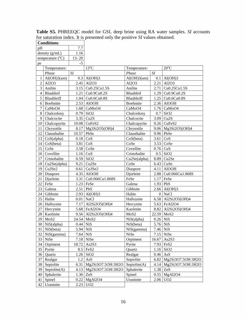
Table S5. PHREEQC model for GSL deep brine using RA water samples. SI accounts for saturation index. It is presented only the positive SI values obtained. Conditions: pH 7.7 density (g/mL) 1.16 temperature (oC) 13- 20 pe -5 Temperature: 13oC Temperature: 20oC Phase SI Phase SI

1 Al(OH)3(am) 0.3 Al(OH)3 Al(OH)3(am) 0.1 Al(OH)3 2 Al2O3 2.45 Al2O3 Al2O3 2.21 Al2O3 3 Anilite 3.15 Cu0.25Cu1.5S Anilite 2.71 Cu0.25Cu1.5S 4 BlaubleiI 1.21 Cu0.9Cu0.2S BlaubleiI 1.29 Cu0.9Cu0.2S 5 BlaubleiII 1.04 Cu0.6Cu0.8S BlaubleiII 1.25 Cu0.6Cu0.8S 6 Boehmite 2.53 AlOOH Boehmite 2.36 AlOOH 7 CaMoO4 1.68 CaMoO4 CaMoO4 1.76 CaMoO4 8 Chalcedony 0.79 SiO2 Chalcedony 0.7 SiO2 9 Chalcocite 3.35 Cu2S Chalcocite 3.09 Cu2S

10 Chalcopyrite 10.08 CuFeS2 Chalcopyrite 9.26 CuFeS2 11 Chrysotile 8.17 Mg3Si2O5(OH)4 Chrysotile 9.06 Mg3Si2O5(OH)4 12 Clausthalite 10.57 PbSe Clausthalite 9.96 PbSe 13 CoS(alpha) 0.18 CoS CoS(beta) 3.61 CoS 14 CoS(beta) 3.81 CoS CoSe 3.53 CoSe 15 CoSe 3.58 CoSe Covellite 0.76 CuS 16 Covellite 1.16 CuS Cristobalite 0.5 SiO2 17 Cristobalite 0.59 SiO2 Cu2Se(alpha) 8.89 Cu2Se 18 Cu2Se(alpha) 9.21 Cu2Se CuSe 6.43 CuSe 19 Cu3Se2 0.61 Cu3Se2 Diaspore 4.11 AlOOH 20 Diaspore 4.35 AlOOH Djurleite 2.88 Cu0.066Cu1.868S 21 Djurleite 3.31 Cu0.066Cu1.868S FeSe 1.17 FeSe 22 FeSe 1.23 FeSe Galena 1.93 PbS 23 Galena 2.51 PbS Gibbsite 2.66 Al(OH)3 24 Gibbsite 2.93 Al(OH)3 Halite 0 NaCl 25 Halite 0.01 NaCl Halloysite 6.58 Al2Si2O5(OH)4 26 Halloysite 7.17 Al2Si2O5(OH)4 Hercynite 5.63 FeAl2O4 27 Hercynite 5.68 FeAl2O4 Kaolinite 8.82 Al2Si2O5(OH)4 28 Kaolinite 9.56 Al2Si2O5(OH)4 MoS2 22.59 MoS2 29 MoS2 24.54 MoS2 NiS(alpha) 0.26 NiS 30 NiS(alpha) 0.44 NiS NiS(beta) 5.76 NiS 31 NiS(beta) 5.94 NiS NiS(gamma) 7.46 NiS 32 NiS(gamma) 7.64 NiS NiSe 7.15 NiSe 33 NiSe 7.18 NiSe Orpiment 16.67 As2S3 34 Orpiment 18.72 As2S3 Pyrite 7.93 FeS2 35 Pyrite 8.5 FeS2 Quartz 1.16 SiO2 36 Quartz 1.26 SiO2 Realgar 0.46 AsS 37 Realgar 1.2 AsS Sepiolite 6.82 Mg2Si3O7.5OH:3H2O 38 Sepiolite 6.31 Mg2Si3O7.5OH:3H2O Sepiolite(A) 4.14 Mg2Si3O7.5OH:3H2O 39 Sepiolite(A) 4.13 Mg2Si3O7.5OH:3H2O Sphalerite 1.38 ZnS 40 Sphalerite 1.36 ZnS Spinel 0.55 MgAl2O4 41 Spinel 0.22 MgAl2O4 Uraninite 2.06 UO2 42 Uraninite 2.23 UO2

17

Table S6. Settling velocities and settling times for representative compounds and different nanoparticles sizes.

Representative compound

Particle diameter (nm)

Particle density (g/cm3)

Fluid density (g/cm3)

Settling velocity (cm/s)

Settling time (d)

Settling time (yr)

Boehmite

1000

3.0 1.1

8.7E-05 13.2 0.036 450 1.8E-05 65.4 0.18 250 5.5E-06 211.9 0.6 50 2.2E-07 5298.3 14.5 10 8.7E-09 132456.5 362.9 1 8.7E-11 13245653.7 36289.5 0.5 2.2E-11 52982614.7 145157.8

Boehmite

1000

3.0

1.16

8.47E-05 13.7 0.037 450 1.71E-05 67.5 0.18 250 5.29E-06 218.7 0.6 50 2.12E-07 5467.4 15.0 10 8.47E-09 136683.9 374.5 1 8.47E-11 13668387.3 37447.6 0.5 2.12E-11 55220284.7 151288.5

Pyrite

1000

5.0 1.16

1.73E-04 6.7 0.018 450 3.51E-05 33.0 0.090 250 1.08E-05 106.8 0.3 50 4.34E-07 2669.8 7.3 10 1.73E-08 66744.3 182.9 1 1.73E-10 6674433.3 18286.1 0.5 4.34E-11 26697733.1 73144.5

18

Figure S1. Average total concentrations of trace metals in raw acidified samples (RA) and filtered acidified samples (FA) taken at four stations (2267, 2767, 2565 and 3510) and different depths (0.2, 3.0, 6.5 and 8.0 m). RA represents dissolved + particulate concentrations; whereas FA represents dissolved concentrations.

19

Fractogram for carboxylated PS (98 & 200nm) and gold colloid (10 nm) nanoparticles

-0,01

0

0,01

0,02

0,03

0,04

0,05

0,06

0 5 10 15 20

Time (min)

Inte

nsity

UV

Void

10 nm

98 nm

200 nm

Calibration curve for nanoparticles

dh = 17.748 tr - 132.55R2 = 0.974

0

50

100

150

200

250

0 2 4 6 8 10 12 14 16 18 20Retention time (min)

Hyd

rody

nam

ic d

iam

eter

(nm

)

Injection/transition

Figure S2. Calibration curve for latex beads and colloidal gold nanoparticles for a size range of 10 to 250 nm.

20

Fractogram using Polystyrene Sulfonate Standards (PSS)

0

0,05

0,1

0,15

0,2

0,25

0 5 10 15 20

Time (min)

Inte

nsity

UV

Void

0.9 1.6 2.4 4.9 Size

8K 18K 35K 100K MW

Calibration curve for macromolecules

dh = 0.4382 tr - 2.4389R2 = 0.9988

0

1

2

3

4

5

6

0 5 10 15 20Retention time (min)

Hyd

rody

nam

ic d

iam

eter

(nm

)

Injection/transition

Figure S3. Calibration curve for polystyrene sulfonates standards (PSS) for a size range of 0.9 to 5 nm

21

Figure S4a. Fractograms of the milli-Q water for size range: 10 – 250 nm.

22

Figure S4b. Fractograms of the GSL synthetic for size range: 10 – 250 nm.

23

Figure S5a. Fractograms of the milli-Q water for size range: 0.9 – 7.5 nm.

24

Figure S5b. Fractograms of the GSL synthetic for size range: 0.9 – 7.5 nm.

25

Predicted phases using GSL shallow brines

0.01

0.1

1

10

100Al

OO

HAl

OO

HAl

(OH

)3Fe

Al2O

4Ba

3(As

O4)

2Ba

SO4

CaM

oO4

U3O

8U

4O9

UO

2Si

O2

Mg3

Si2O

5(O

H)4

SiO

2Al

2Si2

O5(

OH

)4Al

2Si2

O5(

OH

)4Si

O2

Mg2

Si3O

7.5O

H:3

H2O

Mg2

Si3O

7.5O

H:3

H2O

CoF

e2O

4C

uFe2

O4

CuF

eO2

Fe(O

H)2

.7C

l.3Fe

OO

HFe

2O3

Fe2O

3Fe

2MgO

4Fe

3O4

Satu

ratio

n in

dex

Predicted phases using GSL deep brines

0.01

0.1

1

10

100

Al(O

H)3

Al2O

3Al

OO

HAl

OO

HAl

(OH

)3M

gAl2

O4

FeAl

2O4

CaM

oO4

UO

2Si

O2

Mg3

Si2O

5(O

H)4

SiO

2Al

2Si2

O5(

OH

)4Al

2Si2

O5(

OH

)4Si

O2

Mg2

Si3O

7.5O

H:3

H2O

Mg2

Si3O

7.5O

H:3

H2O

NaC

lC

u0.2

5Cu1

.5S

Cu0

.9C

u0.2

SC

u0.6

Cu0

.8S

Cu2

SC

uFeS

2C

oSC

oSC

uSC

u0.0

66C

u1.8

68S

PbS

MoS

2N

iSN

iSN

iSAs

2S3

FeS2 AsS

ZnS

PbSe

CoS

eC

u2Se

Cu3

Se2

FeSe

NiS

e

Satu

ratio

n in

dex

Figure S6. Predicted precipitate phase using USGS PHREEQC software. Top: shallow brine. Bottom: deep brine.

26

Figure S7. Trace metals trajectories for the shallow brines represented by site 2565 at 0.2 m.

27

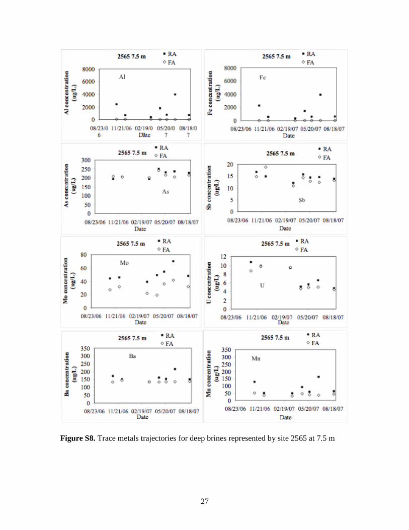
Figure S8. Trace metals trajectories for deep brines represented by site 2565 at 7.5 m