Single Particle, Passive Microrheology in Biological Fluids with Drift

John W. R. Mellnik

Curriculum in Bioinformatics and Computational Biology, Department of Mathematics,

Department of Biomedical Engineering, University of North Carolina at Chapel Hill, Chapel Hill,

NC 27599, USA

Path BioAnalytics, Inc. Chapel Hill, NC 27510

Martin Lysy

Department of Statistics and Actuarial Science, University of Waterloo, Waterloo, ON N2L 3G1,

Canada

Paula A. Vasquez

Department of Mathematics, University of South Carolina, Columbia, SC 29208, USA

Natesh S. Pillai

Department of Statistics, Harvard University, Cambridge, MA 02138, USA

David B. Hill

The Marsico Lung Institute, Department of Physics and Astronomy, University of North Carolina

at Chapel Hill, Chapel Hill, NC 27599, USA

Jeremy Cribb

Department of Physics and Astronomy, University of North Carolina at Chapel Hill, Chapel Hill,

NC 27599, USA

Scott A. McKinley

Department of Mathematics, Tulane University, New Orleans, LA 70118, USA

M. Gregory Forest

Department of Mathematics, Department of Biomedical Engineering, University of North

Carolina at Chapel Hill, Chapel Hill, NC 27599, USA

Synopsis

Volume limitations and low yield thresholds of biological fluids have led to widespread use of

passive microparticle rheology. The mean-squared-displacement (MSD) statistics of bead

position time series (bead paths) are transformed to determine dynamic storage and loss

moduli [Mason and Weitz (1995)]. A prevalent hurdle arises when there is a non-diffusive

experimental drift in the data. Commensurate with the magnitude of drift relative to diffusive

mobility, quantified by a Péclet number, the MSD statistics are distorted, and thus the path

data must be “corrected” for drift. The standard approach is to estimate and subtract the drift

from particle paths, and then calculate MSD statistics. We present an alternative, parametric

approach using maximum likelihood estimation (MLE) that simultaneously fits drift and diffusive

model parameters from the path data; the MSD statistics (and dynamic moduli) then follow

directly from the best-fit model. We illustrate and compare both methods on simulated path

data over a range of Péclet numbers, where exact answers are known. We choose fractional

Brownian motion as the numerical model because it affords tunable, sub-diffusive MSD

statistics consistent with several biological fluids. Finally, we apply and compare both methods

on data from human bronchial epithelial cell culture mucus.

I. INTRODUCTION

Particle tracking microrheology focuses on the movement of tracer particles embedded in the

fluid of interest [Qian et al. (1991); Crocker and Grier (1994); Crocker et al. (2000); Levine and

Lubensky (2002); Gardel et al. (2003); Weihs et al. (2006); Crocker and Hoffman (2007);

Hohenegger and Forest (2008); Houghton et al. (2008); Aufderhorst-Roberts et al. (2012);

Bertseva et al. (2012); Tassieri et al. (2012); Fong et al. (2013); Gal et al. (2013); Hill et al. (2014)]

while “endogenous” microrheology analyzes the motion of particulates or cellular constituents

[Dieterich et al. (2008); Bronstein et al. (2009); Kenwright et al. (2012); Verdaasdonk et al. (2013);

Mak et al. (2014)] in situ. Particle tracking microrheology can be subdivided into passive [ Qian et

al. (1991); Gardel et al. (2003); Houghton et al. (2008); Aufderhorst-Roberts et al. (2012); Fong et

al. (2013); Hill et al. (2014)] (where particle motion arises from thermal fluctuations) and active

[Crocker and Grier (1994); Bertseva et al. (2012); Tassieri et al. (2012); Cribb et al. (2013)] (where

the particles are manipulated by an external force). Two-particle, also known as two-point,

microrheology [Crocker et al. (2000); Levine and Lubensky (2002); Crocker and Hoffman (2007);

Hohenegger and Forest (2008)] focuses on the auto- and cross-correlations of particle pairs as a

means to screen uniform drift or to screen the modified fluid properties due to chemical

interactions of the probe particle with the host fluid sample. In some fluids, however,

concentrations required to get sufficient nearby pairs of particles can modify the sample

properties.

Faithful inference of the linear viscoelastic properties of a host fluid via single particle passive

microrheology requires that particles are sufficiently dispersed and have neutral interactions

with the surrounding medium. Passive microrheology is employed to infer the diffusive mobility

of foreign particles of diverse size and surface chemistry, e.g., for controlled delivery of drug

carrier particles through mucus barriers (cf. the recent review article by Schuster et al.

(2015)). Uniting all of these applications of passive microbead microrheology is the analysis of

the mean squared displacement (MSD) statistics of a tracked particle in order to estimate either

the particle’s diffusive transport properties or the physical viscoelastic properties of the particle’s

local environment [Mason (2000)]. The analysis of the MSD in this context stems from the seminal

work of Einstein (1905) for viscous fluids where the MSD scales linearly with time, and the pre-

factor 𝐷 provides a direct inference of the fluid viscosity 𝜂 given the temperature 𝑇 and

hydrodynamic radius 𝑎 of the probe, 𝐷 = 𝑘𝐵𝑇(6𝜋𝜂𝑎)−1, where 𝑘𝐵 is the Boltzmann constant.

The primary application that motivates this work is the determination of the linear viscoelastic

properties (frequency-dependent dynamic storage and loss moduli) of biological soft matter, and

human mucus in particular. Inferring linear viscoelastic moduli involves the MSD of tracked

passive microbead position time series (which we refer to as “paths”) coupled with the Mason-

Weitz protocol [Mason and Weitz (1995); Mason (2000)]. Video microscopy in combination with

passive microbead particle tracking (MPT) has been used to explore the physical properties of a

wide range of mucus biogels, including cervicovaginal [Lai et al. (2009); das Neves et al. (2012);

Wang et al. (2013)] pulmonary [Hill et al. (2014); Schuster et al. (2015)] and gastrointestinal

[Georgiades et al. (2014a); Georgiades et al. (2014b); Macierzanka et al. (2014)] mucus. Often

in passive MPT experiments, the observed particles exhibit drift: a persistent, inadvertent, driven

motion potentially due to the light source [Schuster et al. (2015)], movement of the optical stage

[Adler and Pagakis (2003); Dangaria et al. (2007)], or some other source [Aufderhorst-Roberts et

al. (2014)]. Thus the particle observations are a superposition of drift and diffusion. In active

biological fluids such as living cells where endogenous DNA domains are fluoresced and tracked,

cell translocation and active cellular processes induce additional forcing. In viral trafficking within

cells, the virus may hijack directed motion along microtubules. Since drift can significantly alter

the MSD of tracked particles, and thereby distort the inference of the viscous and elastic moduli

of the particle’s local environment [Mason et al. (1995); Mason et al. (1997)], as well as distort

the inferred mobility, the question naturally arises as to how drift should be accounted for in the

analysis of MPT data.

In the case of optical stage drift, each particle in the field of view exhibits the same magnitude

and direction of movement. Thus, if enough particles are present, the driven motion may be

removed by estimating the ensemble average movement of the particles within the field of view

and subtracting this drift from each particle path [Hasnain and Donald (2006)]. Other scenarios

pose a more difficult challenge due to the potential for temporal and spatial heterogeneity in the

drift force. In highly heterogeneous biological fluids such as mucus, regions of high elasticity, due

to high local mucin concentrations, may cause some particles to appear immobile while

neighboring particles are clearly undergoing net transport due to some local flow. In this scenario,

if one were to subtract the ensemble-averaged movement of the particles in the field of view

from each particle path, one would be adding directed motion to the less mobile particles while

subtracting directed motion from the more mobile particles. In Fong et al. (2013) the authors

introduce a "de-trending" method for Brownian motion in heterogeneous fluids that is applied

to each particle path individually, where the data is reduced by half through restricting analysis

to the movement orthogonal to the estimated drift direction. Here we also analyze individual

paths, allowing for independent drift per path, for both Brownian and fractional Brownian

motion. In Lysy et al. (2014) a de-trending method is applied to a larger class of diffusive and

sub-diffusive processes with drift in two space dimensions, where the full 2d observations are

used to simultaneously estimate the diffusive or sub-diffusive model parameters and the drift.

The present article aims to introduce and illustrate the parametric, maximum likelihood

estimation approach in one-dimensional data; for a more rigorous treatment, including

comparisons of competitive models on the basis of the available data, see Lysy et al. (2014).

We point out that the debate over the optimal way to remove drift tacitly assumes that directed

motion must be removed prior to analyzing the path data. Historically, this assumption is natural

because of the focus on the scaling of the ensemble particle MSD due to purely diffusive dynamics

[Einstein (1905); Qian et al. (1991); Michalet (2010); Gal et al. (2013)], a statistic that can be

extremely sensitive to drift [Weihs et al. (2007)] In this article, we take a different approach and

show that deterministic drift does not need to be removed a priori from particle path data to

determine the MSD statistics if one posits and exploits a fully parametric statistical model for the

underlying drift-diffusion process. In particular, we focus on fractional Brownian motion (fBm), a

parametric statistical model for sub-diffusive processes that has been shown to accurately

describe diffusion in mucus gels [Hill et al. (2014); Lysy et al. (2014)] and other biological soft

matter [Kou et al. (2004); Kou et al. (2008)]. Using numerical simulations of drift coupled with

sub-diffusive fractional Brownian motion (consistent with data from mucus gels), we show that

one can easily and accurately estimate the diffusive or sub-diffusive model parameters by

maximum likelihood estimation (MLE) -- for a wide range of deterministic drift, and without

removing the drift a priori as is typically done to estimate the MSD statistics of single or ensemble

paths. The advantage of MLE arises because drift is treated as a model parameter to be estimated

jointly with the diffusive or sub-diffusive parameters rather than sequentially, thereby increasing

the precision of all parameter estimates. With all parameters thus estimated jointly, it is then

straightforward to use fBm parameter estimates to generate the MSD of the purely diffusive

dynamics and thereby infer the dynamic viscoelastic moduli by the Mason-Weitz protocol. We

illustrate the procedure for a range of Péclet numbers by introducing a dimensionless ratio of the

drift (advection) component relative to the diffusive mobility, for both normal and sub-diffusive

processes.

The benefit of numerical simulation is that the exact diffusive parameters and linear viscoelastic

moduli are known, so that the error induced by relative drift (parametrized by Péclet number),

for any method of estimating these quantities, can be directly measured and compared to any

other method. We are thus able to compare the errors in the inference of diffusive process

parameters and in dynamic storage and loss moduli among our proposed parametric maximum

likelihood estimation method and the standard approach in the passive microrheology literature

based on a least-squares estimate of the MSD after removal of drift. We also show, for posterity,

the dramatic errors in the diffusion parameters and viscoelastic moduli if one simply ignores the

presence of drift. Finally, we apply MLE and the standard drift-subtracted MSD estimate

approaches to experimental particle path data in human bronchial epithelial cell culture mucus.

The structure of the article is as follows. First, we discuss drawbacks of MSD-based approaches

and cursory drift removal. We then introduce a canonical model (fractional Brownian motion) for

tunable particle diffusion or sub-diffusion with drift, and provide details on how to simulate

particle paths in accordance with this model. Next, we review MSD-based approaches to the

recovery of diffusive parameters and present our MLE method. The methods are then compared

on simulated data sets for a practical range of Péclet numbers. Finally we illustrate the methods

on data from human lung cell culture mucus.

II. MEAN SQUARED DISPLACEMENT STATISTICS

Give observations 𝑋(0), 𝑋(∆𝑡), 𝑋(2∆𝑡), … , 𝑋(𝑀∆𝑡) of a particle’s position, the MSD statistic is

calculated as

⟨𝑟𝜏⟩2 =

1

𝑀 − 𝑖 + 1∑[𝑋(𝑖∆𝑡 + 𝑗∆𝑡) − 𝑋(𝑗∆𝑡)]2,

𝑀−𝑖

𝑗=0

(1)

where 𝜏 = 𝑖∆𝑡 is the lag time and ∆𝑡 is the time between observations. For many diffusive

processes, theory and observation suggest that the MSD of particles undergoing diffusion

exhibits a power law scaling: [Caspi et al. (2000); Mason (2000); Seisenberger et al. (2001);

Valentine et al. (2001); das Neves et al. (2012); Hill et al. (2014)]

𝐸[⟨𝑟𝜏⟩2] = 2𝑑𝐷𝜏𝛼, (2)

where the prefactor 𝐷 is the “diffusivity” by analogy with simple diffusion, 𝛼 is a real number in

the interval [0, 2], and 𝑑 is the dimensionality. For standard Brownian motion without drift, the

power-law exponent is 𝛼 = 1. From an accurate estimation of 𝐷 one infers the fluid viscosity 𝜂

from the Stokes-Einstein relation. Weihs et al. (2007) illustrated via simulated Brownian motion

that linear (i.e. constant) drift causes a log-log plot of MSD versus lag time 𝜏 to tend toward a

slope of 2 at large lag times (Figure 1). That is, as 𝜏 increases, 𝛼 → 2 and the larger the drift

velocity, the smaller the lag time at which this transition occurs.

When one attempts to correct for directed motion by subtracting the mean increment, i.e., the

mean of the step-size distribution at the shortest lag time (Figure 2), one inadvertently changes

the structure of the entire particle path; e.g., every such modified path is constrained to begin

and end at the same spatial position. To see this, consider a one-dimensional Brownian path,

where 𝑋𝑖 = 𝑋(𝑖∆𝑡) is the location of the particle at time 𝑖∆𝑡 with 𝑖 = 1, 2, 3 … 𝑀. The increments

of this process are given by

𝑥𝑖 = 𝑋𝑖+1 − 𝑋𝑖 . (3)

For Brownian motion, the 𝑥𝑖 are normally distributed with mean 𝜇∆𝑡 and variance 2𝐷∆𝑡, where

𝜇 is the drift velocity. When no drift is present, the sample mean of 𝑥𝑖,

�̅� =

1

𝑀 − 1∑ 𝑥𝑖

𝑀−1

𝑖=1

, (4)

converges to zero as the number of particle positions increases, i.e. as 𝑀 → ∞. The fact that the

distribution of 𝑥𝑖 is symmetric with �̅� converging to zero intuitively indicates that the particle is

expected to make an equal number of steps to the left and right. This however, is not to say that

a particle diffusing via Brownian motion never travels a net distance. The mean incremental

displacement is �̅�, and when we subtract �̅� from each increment, 𝑥𝑖, we “snap” the distribution

of 𝑋𝑀 to zero, inadvertently stipulating that the first and final positions of the particle are the

same. Indeed, suppose that �̅� is subtracted from each increment to “remove drift,” centering the

distribution of increments at zero. The resulting modified position process is computed by taking

the cumulative sum of the shifted increments, denoted by �̃�𝑖,

�̃�1 = 𝑋1 �̃�2 = 𝑋1 + (𝑥1 − �̅�) �̃�3 = 𝑋1 + (𝑥1 − �̅�) + (𝑥2 − �̅�) �̃�4 = 𝑋1 + (𝑥1 − �̅�) + (𝑥2 − �̅�) + (𝑥3 − �̅�) ⋮

(5)

Following this pattern, we collect terms and write the final position �̃�𝑀 as,

�̃�𝑀 = 𝑋1 − (𝑀 − 1)�̅� + ∑ 𝑥𝑖 ,

𝑀−1

𝑖=1

(6)

which can be simplified further,

�̃�𝑀 = 𝑋1 − (𝑀 − 1)

1

𝑀 − 1∑ 𝑥𝑖

𝑀−1

𝑖=1

+ ∑ 𝑥𝑖

𝑀−1

𝑖=1

(7)

�̃�𝑀 = 𝑋1 − ∑ 𝑥𝑖

𝑀−1

𝑗=1

+ ∑ 𝑥𝑖

𝑀−1

𝑖=1

(8)

�̃�𝑀 = 𝑋1 (9)

and thus we see that the final position has been constrained to the initial position (Figure 3). It

is worth noting that a standard Brownian motion constrained to have coincident initial and final

positions is called a Brownian bridge [Steele (2001)], which has completely different correlation

structure than the unconstrained motion. While this does not make a difference in the estimation

procedure if the paths are from a standard Brownian motion (and thus the increments are

independent), it becomes relevant when the paths are from fractional Brownian motion where

the increments may be highly correlated.

An additional drawback of an MSD-based approach to diffusive parameter estimation is the

unreliability in the MSD at large lag times. As the lag time increases, the number of increments

included in the mean of the squared increments decreases and thus becomes less stable. Weihs

et al. (2007) estimate that only the initial two-thirds of the MSD is statistically reliable. Due to

experimental factors (particles exiting the focal plane of the microscope) limiting the ability to

collect data over long time scales, the uncertainty in the MSD for large lag times can have a

pronounced impact on the accurate recovery of diffusive and viscoelastic properties.

Figure 1: Path-wise MSD for simulated particles from the Brownian motion (Bm) (a) and fractional Brownian motion (fBm) (b). MSD curves for 40 representative data sets are shown for varying drift characterized by the Péclet number (Pe), the ratio of the advective and diffusive transport rates (Eqn. (13)). The color scheme represents increasing Péclet from 𝑃𝑒𝑚𝑖𝑛 = 0 (blue) to 𝑃𝑒𝑚𝑎𝑥 = 0.73 (red), for the Bm data set, and from 𝑃𝑒𝑚𝑖𝑛 = 0 (blue) to 𝑃𝑒𝑚𝑎𝑥 = 0.52 (red) for the fBm data set. The upper and lower black dashed lines indicate slopes of 2 (ballistic motion) and 1 (normal diffusion), respectively. The fBm paths (b) are simulated with 𝛼 = 0.6; the "diffusivity" pre-factor is chosen to have the same numerical value in the two data sets.

Figure 2: Impact of drift-subtraction on the distribution of increments and MSD for a representative sub-diffusive fractional Brownian motion path with true parameter values 𝛼 = 0.60 and 𝐷 = 4.67 × 10−4 𝜇𝑚2𝑠−𝛼. The estimated parameter values based on a simple least-squares fit to the drift subtracted MSD are 𝛼 = 0.53 and 𝐷 =5.30 × 10−4 𝜇𝑚2𝑠−𝛼. The distribution of increments (a) is shown at 𝜏 = 5 s for a single particle path with 𝑃𝑒 = 0.5 before (blue) and after (red) drift subtraction. Before drift subtraction, the mean of the distribution of increments (solid blue line) is 9.40 × 10−3 𝜇𝑚. Subtracting drift centers the distribution at zero (solid red line). The MSD is also shown for this path before and after drift subtraction (b).

Figure 3: Sample Brownian path with drift (a) and after the drift has been removed by subtracting the mean displacement from each increment (b). The beginning and end of the path have been marked with a blue x and a red circle, respectively.

III. FRACTIONAL BROWNIAN MOTION AND DRIFT

Recently, Lysy et al. (2014) considered fractional Brownian motion (fBM) as a model for the

movement of micron-scale particles over a 30 second observation time at 60 frames per second

temporal resolution in human bronchial epithelial mucus. Under this model, the particle's

position process 𝑋(𝑡) in one dimension is written as the sum of a deterministic term representing

the drift and a stochastic term representing the particle’s thermally activated diffusive

movements:

𝑋(𝑡) = 𝜇𝑡 + √2𝐷𝑊𝛼(𝑡), (10)

where 𝑊𝛼(𝑡) is a continuous Gaussian process with mean zero and covariance

𝑐𝑜𝑣[𝑊𝛼(𝑡), 𝑊𝛼(𝑠)] =1

2(|𝑡|𝛼 + |𝑠|𝛼 − |𝑡 − 𝑠|𝛼), 0 < 𝛼 < 2. (11)

For 𝛼 = 1, Eqn. (10) reduces to Brownian motion with drift, and the increment process is

uncorrelated: 𝑐𝑜𝑣[𝑥𝑖 , 𝑥𝑖+𝑘] = 𝐷∆𝑡. For 𝛼 ≠ 1, the increment process for fBm has correlation

𝑐𝑜𝑣[𝑥𝑖 , 𝑥𝑖+𝑘] = 𝐷∆𝑡𝛼(|𝑘 + 1|𝛼 + |𝑘 − 1|𝛼 − 2|𝑘|𝛼). (12)

For fBm processes, the MSD has the same scaling relation as Brownian motion [Mandelbrot and

Van Ness (1968)], i.e., ⟨𝑟𝜏⟩2~𝐷𝜏𝛼, although, unlike Brownian motion, the power-law exponent is

not necessarily unity. When 𝛼 < 1, the fBm increments are negatively correlated and the

position process exhibits subdiffusive behavior. When 𝛼 > 1, the fBm increments are positively

correlated and the position process exhibits superdiffusive behavior.

Calculating the increments 𝑥𝑖 provides a simple way to estimate the drift exhibited by a particle

since the mean, or expected value, of the increments is 𝐸[𝑥𝑖] = 𝜇∆𝑡, for both Brownian and

fractional Brownian processes. To generalize our analysis, we characterize results in terms of a

Péclet number (𝑃𝑒), a dimensionless ratio of the advective and diffusive transport rates. Given

the increments of a particle path computed for a given lag time ∆𝑡, our choice of Péclet number

is calculated by dividing the mean increment, 𝐸[𝑥𝑖] or the expectation of 𝑥𝑖, by the standard

deviation 𝑆𝐷[𝑥𝑖] of the increments,

𝑃𝑒 ≡

𝐸[𝑥𝑖]

𝑆𝐷[𝑥𝑖].

(13)

IV. SIMULATION DESIGN

To generate a particle path exhibiting linear drift and fractional Brownian dynamics, we first

generate the increment process for an fBm path without drift, then add the desired drift to the

path. To generate fBm observations 𝑋1,…, 𝑋𝑀 for a particular choice of 𝛼, we first construct the

covariance matrix 𝑺 of the increment process according to Eqn. (12). That is, the 𝑖, 𝑗𝑡ℎ elements

of 𝑺 is

𝑺𝑖,𝑗 = 𝑐𝑜𝑣[𝑥𝑖 , 𝑥𝑗] (14)

for 𝑖, 𝑗 = 1, 2, … 𝑀. Let 𝑳𝑳′ = 𝑺 be the Cholesky decomposition of 𝑺 and let 𝒖 be a vector of M

independent and identically distributed draws from a standard normal distribution. A simulated

particle path is generated as 𝑥 = √2𝐷𝑳𝒖, 𝑋𝑗 = ∑ 𝑥𝑖𝑗𝑖=1 . Using this method, two sets of simulated

data are generated. The first set is subdiffusive with 𝛼 = 0.6 and 𝐷 = 4.67 × 10−4 μm2s−α,

mimicking the estimated parameter values based on experimental observations of 1 μm

diameter particles in 4 weight percent human bronchial epithelial mucus [Hill et al. (2014)]. The

second data set has the same numerical value of the diffusivity as the subdiffusive data set, but

exhibits standard Brownian motion, i.e., 𝛼 = 1 and 𝐷 = 4.67 × 10−4 μm2s−1. This diffusivity

corresponds to a 1 μm diameter particle in a fluid with viscosity of 1.86 Pa s at 23 °C. Each

simulated path is generated with a temporal resolution of 5 frames per second and a length of

𝑀 = 2,992 steps, mimicking experimental conditions for the experimental data presented in

Section VII.

Linear drift is added to the simulated paths by calculating the increments, adding directed

motion, then taking the cumulative sum of the result. We consider directed motion up to twenty

times the diffusivity of the particle, matching the range in drift observed in experimental data

(Section VII). Therefore, a position process with linear drift is given by,

𝑋𝑗 = ∑(𝑥𝑖

𝑗

𝑖=1

+ 𝐷𝛬),

(15)

where 𝛬 is a scaling factor with units sαμm−1. We generate 100 simulated paths with drift for 𝛬

spanning the interval [0, 20] in increments of 0.5 sαμm−1, resulting in 4,100 simulated fBm paths

(𝛼 = 0.6) and 4,100 simulated Brownian paths (𝛼 = 1). These data sets will be referred to as

the fractional Brownian motion (fBm) and Brownian motion (Bm) data sets. The Péclet number

for the Bm data set ranged from 0 to 0.73 and 0 to 0.52 for the fBm data set.

V. APPROACHES TO PARAMETER ESTIMATION

We consider three approaches to diffusive parameter estimation.

Simple least squares Noting that the subdiffusive MSD is linear on the log-scale,

log(𝐸[⟨𝑟𝜏⟩2]) = log(2𝐷) + 𝛼log (𝜏),

a longstanding approach to estimate 𝐷 and 𝛼 is to minimize the least squares (𝐿𝑆) objective

function

∑ (𝑦𝑖 − 𝑐 − 𝛼𝑡𝑖)2𝑀𝑖=1 , (16)

in terms of 𝑐 and 𝛼 where,

𝑦𝑖 = ln[⟨𝑟𝜏⟩𝑖2

], c = ln[2𝐷], 𝑡𝑖 = ln[𝜏𝑖]. (17)

The minimum of Eqn. (16) is obtained at �̃� = ∑ 𝑦𝑖𝑡𝑖𝑀𝑖=1 ∑ 𝑡𝑖

2𝑀𝑖=1⁄ and �̃� = �̅� − �̃�𝑡̅.

Drift-Subtracted Least Squares The drift-subtracted least squares (𝐷𝐿𝑆) approach

subtracts �̅�, the mean increment, from each 𝑥𝑖, centering the distribution of increments at zero,

constraining the equivalence of the initial and final position, before applying the approach

described above for least squares estimation.

Full Model MLE This approach applies maximum likelihood estimation (𝑀𝐿𝐸) to Eqn. (10)

to estimate 𝜇, 𝐷 and 𝛼 directly from the raw data without first estimating the MSD statistic. The

fBm model (10) specifies that the increments 𝑥𝑖 have a multivariate Gaussian distribution,

𝑥~𝑁(𝜇∆𝑡, 𝜎2𝑉𝛼), 𝜎2[𝑉𝛼]𝑖,𝑗 = 𝑐𝑜𝑣[𝑥𝑖 , 𝑥𝑖+(𝑗−𝑖)], (18)

where 𝑐𝑜𝑣[−] is given by Eqn. (11) and 𝜎 = 2𝐷. The likelihood function is thus ℒ(𝜃|𝑥) = 𝑝(𝑥|𝜃),

the probability of observing the data given the model parameters 𝜃 = (𝜇, 𝜎, 𝛼). The MLE of the

model parameters is denoted 𝜃 = argmax𝜃ℒ(𝜃|𝑥), the value of 𝜃 which maximizes ℒ(𝜃|𝑥). The

three-dimensional optimization problem can be reduced to a one-dimensional problem by

maximizing in (𝜇, 𝜎) for fixed 𝛼. That is, let

𝑦 = [𝑉𝛼]−1/2𝑥 and 𝑧 = ∆𝑡[𝑉𝛼]−1/21𝑀, (19)

where 1𝑀 = (1, 1, … 1). Then we have

𝑦𝑖 = 𝜇𝑧𝑖 + 𝜀𝑖 𝜀𝑖 ~𝑖𝑖𝑑 𝑁(0, 𝜎2).

such that the likelihood function ℒ𝛼(𝜇, 𝜎|𝑥) for fixed 𝛼 is

exp [

−1

2𝜎2∑(𝑦𝑖 − 𝜇𝑧𝑖)2 − Mlog(σ) ].

Therefore, the values (�̂�𝛼 , �̂�𝛼) that maximize ℒ𝛼(𝜇, 𝜎|𝑥) are

�̂�𝛼 =∑ 𝑧𝑖𝑦𝑖

𝑀𝑖=1

∑ 𝑧𝑖2𝑀

𝑖=1

, �̂�𝛼 = (∑ (𝑦𝑖 − �̂�𝛼𝑧𝑖)2𝑀

𝑖=1

𝑀)

1/2

.

The MLE of 𝛼 for Eqn. (10) is then obtained by maximizing the one-dimensional profile likelihood

[e.g., Davidson (2003)] function

ℒprof(𝛼|𝑥) = ℒ(�̂�𝛼 , �̂�𝛼 , 𝛼|𝑥).

Specifically, we find the �̂� that maximizes ℓprof(𝛼|𝑥) = log (ℒprof(𝛼|𝑥)), where

ℓprof(𝛼|𝑥) = −1

2[𝑀log(�̂�𝛼

2) + log(|𝑉𝛼|)].

The resulting parameter estimates 𝜃 = (�̂��̂� , �̂�, �̂��̂�) are precisely those that maximize the full

likelihood ℒ(𝜃|𝑥), thereby reducing the numerical optimization problem from three parameters

to one. Moreover, we note that for arbitrary variance matrix 𝑉, the linear systems in Eqn. (19)

are solved in 𝑂(𝑀3) operations. However, since 𝑉𝛼 is a Toeplitz matrix [Bareiss (1969)], the

systems can be solved in 𝑂(𝑀2) operations using the Durbin-Levinson algorithm [Durbin (1960);

Ljung (1987)].

Much like the least squares approach involving the sample MSD, the maximum likelihood

approach we have described hinges on the minimization of a quadratic objective function.

However, whereas the least squares approach estimates the drift only once, the MLE estimates

the "optimal" drift and diffusivity for every value of 𝛼. That is, the least squares estimate of the

drift by �̅� would be optimal if the increments were uncorrelated, whereas the MLE approach

estimates the drift by a weighted average of the increments, �̂�𝛼 that accounts for their

correlation. Indeed, �̂�𝛼 = �̅� only when fBm reduces to ordinary diffusion with 𝛼 = 1.

VI. RESULTS: Simulated Data

For each simulated path, we compute the path-wise MSD given by Eqn. (1). To estimate the

viscous and elastic moduli, we follow Mason and Weitz (1995) where the complex modulus is

𝐺∗(𝜔) = 𝑖𝜔𝜂∗(𝜔) = 𝐺′(𝜔) + 𝑖𝐺′′(𝜔) =

𝑘𝐵𝑇

𝜋𝑎𝑖𝜔𝔉{⟨𝑟𝜏⟩2}, (20)

where 𝔉{𝑔(𝜏)} = ∫ 𝑔(𝜏)𝑒−𝜔𝑖⋅𝜏𝑑𝜏 denotes the Fourier transform. Note, the dynamic viscosity

𝜂′(𝜔) is related to the viscous modulus via 𝜔𝜂′(𝜔) = 𝐺′′(𝜔).

Figure 4 shows pathwise estimates of the diffusivity 𝐷 and the power-law exponent 𝛼 as a

function of the Péclet number (𝑃𝑒) over the range 𝑃𝑒 = [0, 0.73] using the three methods

described in Section V. The solid red line in each panel is the value used to generate the simulated

data, which is reasonably recovered by each technique when no drift is present, i.e. 𝑃𝑒 = 0. For

Brownian paths when drift is present, ignoring drift completely leads to dramatically incorrect

results. In Figure 5, the relative error in the estimation of the viscosity for the Bm data found by

applying the Stokes-Einstein relation is reported for each estimation approach. The mean relative

error in the estimation of the viscosity when not accounting for drift is 39.5%. When applying a

drift-subtracted least squares (𝐷𝐿𝑆) approach and a parametric 𝑀𝐿𝐸 approach the mean relative

error is 11.1% and 3.6%, respectively.

Figure 6 illustrates the impact of drift on the pathwise estimates of 𝐺′ and 𝐺′′ for the fBm data

for various values of 𝑃𝑒. In Figure 7, the ensemble average estimates 𝐺′ and 𝐺′′ are compared

when applying Eqn. (20) to the empirical MSD when ignoring drift and subtracting drift, and

applying Eqn. (20) to the parametric scaling of the MSD predicted by our 𝑀𝐿𝐸 approach for 𝛬 =

20 sαμm−1, corresponding to 𝑃𝑒 = [0.48, 0.52] for the fBm data. The ensemble average relative

error in the estimation of 𝐺′ and 𝐺′′ for the fBm data set is reported for the 𝐷𝐿𝑆 and 𝑀𝐿𝐸

approaches in Figure 8. This figure shows that the 𝑀𝐿𝐸 method more accurately recovers the

exact 𝐺′ and 𝐺′′, uniformly over all frequencies, whereas the 𝐷𝐿𝑆 method leads to errors in the

low frequency range. The global distortion of individual paths by drift subtraction, the so-called

Brownian bridge, foreshadows the modification of path statistics over long lag times, and

therefore at low frequencies in transform space.

We now turn to the underlying challenge to estimate the diffusivity 𝐷 and the power-law

exponent 𝛼 when the data indicates fractional Brownian motion as a good model. The 𝐿𝑆, 𝐷𝐿𝑆,

and full model 𝑀𝐿𝐸 estimates are shown in Figure 9 as a function of the Péclet number. Recall,

the true values of each parameter are α = 0.6 and 𝐷 = 4.67 × 10−4 μm2s−α. Failing to account

for drift when drift is present leads to highly erroneous results. As 𝑃𝑒 increases, 𝛼 converges to

2, as expected based on the simulation results presented in Figure 1. Drift has a nonlinear impact

on the estimate of 𝐷, initially under-estimating, and later over-estimating the parameter value.

In contrast, both the 𝐷𝐿𝑆 and 𝑀𝐿𝐸 estimates of 𝐷 and 𝛼 are independent of drift and exhibit a

similar level of accuracy, however the parametric approach is the more precise estimator due to

the decreased spread about the mean predicted parameter values.

Figure 4: Estimated values of 𝛼 (a) and 𝐷 (b) ignoring drift (black circles), subtracting drift (blue circles) and our maximum likelihood method (violet circles). The true values of 𝛼 and 𝐷 are shown in solid red lines. The true values of each parameter are 𝛼 = 1 and 𝐷 = 4.67 × 10−4 𝜇𝑚2𝑠−1.

Figure 5: Relative error in estimates of the viscosity (𝜂) given by the Stokes-Einstein relation based on the three approaches for the Brownian motion data set as a function of the Péclet number (Pe). The mean error in the estimation of 𝜂 when not accounting for drift is 39.5%. When applying a drift-subtracted least squares approach and a parametric approach the mean error is 11.1% and 3.6%, respectively.

Figure 6: Pathwise dynamic storage, 𝐺′(𝜔) (a), and loss, 𝐺′′(𝜔) (b) moduli for the fBm data found by transforming the pathwise MSD without accounting for drift. The change in color of the data corresponds to a transition from 𝑃𝑒𝑚𝑖𝑛 = 0 (blue) to 𝑃𝑒𝑚𝑎𝑥 = 0.52 (red). The true values of 𝐺′and 𝐺′′are indicated by the black dashed lines.

Figure 7: Ensemble averaged dynamic storage, 𝐺′(𝜔) (a), and loss, 𝐺′′(𝜔) (b) moduli for the fBm data with subdiffusive exponent 𝛼 = 0.6 by applying Eqn. (20) to the empirical MSD when ignoring drift (black circles) and subtracting drift (blue circles), and applying Eqn. (20) to the parametric scaling of the MSD predicted by our maximum likelihood method (violet circles). Exact 𝐺′(𝜔) and 𝐺′′(𝜔) are shown in solid red lines. The ensemble-averaged results over 100 paths are shown for 𝑃𝑒 values in the range [0.48, 0.52].

Figure 8: Ensemble averaged relative error in the storage modulus, 𝐺′(𝜔) (a), and loss modulus, 𝐺′′(𝜔) (b) for the fBm data with subdiffusive exponent 𝛼 = 0.6 when applying Eqn. (20) to the empirical MSD after subtracting drift (blue) and applying Eqn. (20) to the parametric scaling of the MSD predicted by our maximum likelihood method (violet). The ensemble average is computed using all 4,100 simulated paths.

Figure 9: Estimated values of 𝛼 (a) and 𝐷 (b) ignoring drift (black circles), subtracting drift (blue circles) and our maximum likelihood method (violet circles). The true values of 𝛼 and 𝐷 are shown in solid red lines. The true values of each parameter are 𝛼 = 0.6 and 𝐷 = 4.67 × 10−4 𝜇𝑚2𝑠−𝛼.

VII. RESULTS: Experimental Data

Here, we analyze twenty-two representative 1 μm diameter particles in 4 weight percent human

bronchial epithelial (HBE) mucus using the previously outlined methods. Each path consists of

2,992 increments with a temporal resolution of 0.2 seconds (five observations per second). The

ensemble-averaged storage and loss moduli are calculated when ignoring drift, subtracting drift

by applying Eqn. (20) to the empirical MSD, and applying Eqn. (20) to the parametric scaling of

the MSD of the pure fBm process determined from our maximum likelihood method.

Figure 10: Estimates of the dynamic storage modulus, 𝐺′(𝜔), left figure, and loss modulus, 𝐺′′(𝜔), right figure, for experimental data for 3 approaches: applying Eqn. (20) to the empirical MSD ignoring drift (black circles) and subtracting drift (blue circles), and applying Eqn. (20) to the parametric scaling of the MSD predicted by our maximum likelihood approach (violet circles).

The three estimation methods for 𝐷 and 𝛼 were applied to the experimental particle paths.

Figure 11 shows the least squares (𝐿𝑆) and drift-subtracted least squares (𝐷𝐿𝑆) estimates relative

to the full model maximum likelihood estimation approach (𝑀𝐿𝐸). The estimates for 𝛼 are

presented in Figure 11a. The 𝑀𝐿𝐸 predictions of 𝛼 are shown along the x-axis and the 𝐿𝑆 and

𝐷𝐿𝑆 estimates are shown on the y-axis. The domain of each axis is from 0, representing stuck

particles, to 1, representing normal diffusion exponents. A dashed line indicates the diagonal.

Each data point represents the predicted parameter value for one of the 22 experimental paths.

A data point falling on the diagonal indicates that the 𝑀𝐿𝐸 and 𝐿𝑆 (or 𝐷𝐿𝑆) approaches agree

for that particle path. A data point above the diagonal indicates that the 𝐿𝑆 (or 𝐷𝐿𝑆) approach

overestimated 𝛼 compared to the 𝑀𝐿𝐸 approach. Conversely, a data point below the diagonal

indicates that the 𝐿𝑆 (or 𝐷𝐿𝑆) approach underestimated 𝛼 compared to the 𝑀𝐿𝐸 approach. The

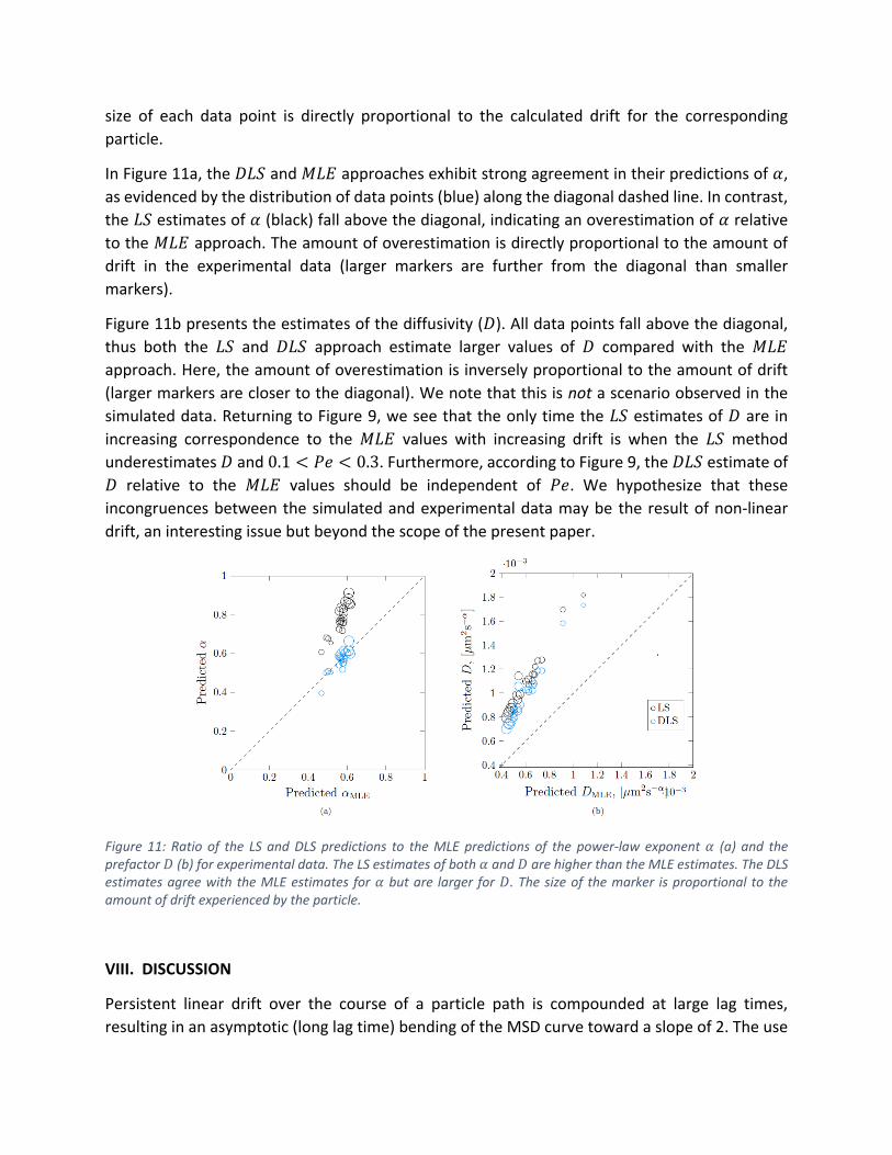
size of each data point is directly proportional to the calculated drift for the corresponding

particle.

In Figure 11a, the 𝐷𝐿𝑆 and 𝑀𝐿𝐸 approaches exhibit strong agreement in their predictions of 𝛼,

as evidenced by the distribution of data points (blue) along the diagonal dashed line. In contrast,

the 𝐿𝑆 estimates of 𝛼 (black) fall above the diagonal, indicating an overestimation of 𝛼 relative

to the 𝑀𝐿𝐸 approach. The amount of overestimation is directly proportional to the amount of

drift in the experimental data (larger markers are further from the diagonal than smaller

markers).

Figure 11b presents the estimates of the diffusivity (𝐷). All data points fall above the diagonal,

thus both the 𝐿𝑆 and 𝐷𝐿𝑆 approach estimate larger values of 𝐷 compared with the 𝑀𝐿𝐸

approach. Here, the amount of overestimation is inversely proportional to the amount of drift

(larger markers are closer to the diagonal). We note that this is not a scenario observed in the

simulated data. Returning to Figure 9, we see that the only time the 𝐿𝑆 estimates of 𝐷 are in

increasing correspondence to the 𝑀𝐿𝐸 values with increasing drift is when the 𝐿𝑆 method

underestimates 𝐷 and 0.1 < 𝑃𝑒 < 0.3. Furthermore, according to Figure 9, the 𝐷𝐿𝑆 estimate of

𝐷 relative to the 𝑀𝐿𝐸 values should be independent of 𝑃𝑒. We hypothesize that these

incongruences between the simulated and experimental data may be the result of non-linear

drift, an interesting issue but beyond the scope of the present paper.

Figure 11: Ratio of the LS and DLS predictions to the MLE predictions of the power-law exponent 𝛼 (a) and the prefactor 𝐷 (b) for experimental data. The LS estimates of both 𝛼 and 𝐷 are higher than the MLE estimates. The DLS estimates agree with the MLE estimates for 𝛼 but are larger for 𝐷. The size of the marker is proportional to the amount of drift experienced by the particle.

VIII. DISCUSSION

Persistent linear drift over the course of a particle path is compounded at large lag times,

resulting in an asymptotic (long lag time) bending of the MSD curve toward a slope of 2. The use

of MSD curves for inference of mobility or linear viscoelastic moduli, without recognizing there is

drift and accounting for it, is obviously problematic. We use a simple calculation of the mean and

standard deviation of the step size distribution for a given experimental or numerical particle

path to determine the drift relative to diffusion, or Péclet number 𝑃𝑒.

When 𝑃𝑒 increases, the slope of the path-wise MSD approaches 2 at increasingly smaller lag

times, causing the least squares (𝐿𝑆) estimate of the power law exponent, 𝛼, to converge to 2.

By subtracting the mean increment of each particle from the particle’s path, the least squares

(𝐷𝐿𝑆) estimate of each parameter is more stable. However, the unanticipated correlation in the

increment process induced by drift subtraction over increasingly large lag times leads to an error

in the estimation of the diffusive parameters that is on the order of 10%. Accordingly, these

discrepancies at large lag times produce errors in the dynamic moduli at low frequencies.

To address this issue, we advocate for a parametric maximum likelihood estimation (𝑀𝐿𝐸)

approach that identifies the best-fit drift parameter 𝜇 simultaneously while estimating 𝐷 and 𝛼.

We demonstrate on numerically generated particle paths, with physically relevant diffusive

parameters from human bronchial epithelial mucus studies, that the use of the parametric

maximum likelihood approach results in approximately a 2/3 reduction in the error in 𝐷 and 𝛼

compared to the standard drift-subtraction least squares approach. These diffusive mobility

parameters are routinely used in drug delivery to compare various drug delivery particle

formulations for passage through mucosal layers [Lai et al. (2009); Wang et al. (2013); Schuster

et al. (2015)]. With respect to inference of linear viscoelasticity from the MSD statistics of particle

paths, we have illustrated that accuracy in storage and loss moduli deteriorates at low

frequencies for the standard drift-subtraction, least squares methods. The gains in accuracy by

the MLE method have been shown for fractional Brownian numerical data typical of

experimentally observed data in mucus gels. Furthermore, we note that the statistical properties

of the 𝑀𝐿𝐸 method are well understood in the statistics community, and have further value

beyond that illustrated here, e.g., for testing model assumptions against experimental data as in

Lysy et al. (2014).

To close, the 𝑀𝐿𝐸, least squares and drift-subtracted least squares parameter estimation

approaches were applied to experimental paths of 1 μm diameter beads in human bronchial

epithelial cell culture mucus [Hill et al. (2014)]. Relative to the parametric maximum likelihood

approach, the drift-subtracted least squares method predicts a higher elasticity above ~0.3 Hz

and a lower viscosity for all frequencies; thus, the standard approach in the literature appears to

bias cell culture mucus toward being more sol-like than gel-like [Winter (1987); Hill et al. (2014)].

IX. ACKNOWLEDGEMENTS

The authors gratefully acknowledge partial support from the National Science Foundation Grants

DMS-1412844, DMS-1100281, DMS-1462992, DMS-1412998, DMS-1410047, DMS-1107070,

National Institutes of Health and National Heart Lung and Blood Institute grants NIH/NHLBI 1 P01

HL108808-01A1, NIH/NHLBI 5 R01 HL 077546-05, and Natural Sciences and Engineering Research

Council of Canada grant RGPIN-2014-04225.

Adler, J. and S. N. Pagakis. 2003. “Reducing Image Distortions due to Temperature-Related Microscope Stage Drift.” Journal of Microscopy 210(2):131–37.

Aufderhorst-Roberts, A., W. J. Frith, and A. M. Donald. 2012. “Micro-Scale Kinetics and Heterogeneity of a pH Triggered Hydrogel.” Soft Matter 8(21):5940–46.

Aufderhorst-Roberts, A., W. J. Frith, M. Kirkland, and A. M. Donald. 2014. “Microrheology and Microstructure of Fmoc-Derivative Hydrogels.” Langmuir 30(15):4483–92.

Bareiss, E. H. 1969. “Numerical Solution of Linear Equations with Toeplitz and Vector Toeplitz Matrices.” Numerische Mathematik 13(5):404–24.

Bertseva, E. et al. 2012. “Optical Trapping Microrheology in Cultured Human Cells.” Eur Phys J E Soft Matter 35(7):63.

Bronstein, I. et al. 2009. “Transient Anomalous Diffusion of Telomeres in the Nucleus of Mammalian Cells.” Phys Rev Lett 103(1):018102.

Caspi, A., R. Granek, and M. Elbaum. 2000. “Enhanced Diffusion in Active Intracellular Transport.” Phys Rev Lett 85(26):5655–58.

Cribb, J. A. et al. 2013. “Nonlinear Signatures in Active Microbead Rheology of Entangled Polymer Solutions.” Journal of Rheology 57(4):1247–64.

Crocker, J. C. et al. 2000. “Two-Point Microrheology of Inhomogeneous Soft Materials.” Phys Rev Lett 85(4):888–91.

Crocker, J. C. and B. D. Hoffman. 2007. “Multiple-Particle Tracking and Two-Point Microrheology in Cells.” Methods Cell Biol 83:141–78.

Crocker, J. C. and D. G. Grier. 1994. “Microscopic Measurement of the Pair Interaction Potential of Charge-Stabilized Colloid.” Phys Rev Lett 73(2):352–55.

Dangaria, J. H., S. Yang, and P. J. Butler. 2007. “Improved Nanometer-Scale Particle Tracking in Optical Microscopy Using Microfabricated Fiduciary Posts.” Biotechniques 42(4):437–40.

Davidson, A. C. 2003. Statistical Models. Vol. 11. Cambridge University Press.

Dieterich, P., R. Klages, R. Preuss, and A. Schwab. 2008. “Anomalous Dynamics of Cell Migration.” PNAS 105(2):459–63.

Durbin, J. 1960. “The Fitting of Time-Series Models.” Review of the International Statistical Institute 28(3):233–44.

Einstein, A. 1905. “On the Movement of Small Particles Suspended in Stationary Liquids Required by the Molecular-Kinetic Theory of Heat.” Annalen der Physik 17:549–60.

Fong, E. J. et al. 2013. “Decoupling Directed and Passive Motion in Dynamic Systems: Particle Tracking Microrheology of Sputum.” Annals of Biomedical Engineering 41(4):837–46.

Gal, N., D. Lechtman-Goldstein, and D. Weihs. 2013. “Particle Tracking in Living Cells: A Review of the Mean Square Displacement Method and beyond.” Rheologica Acta 52(5):425–43.

Gardel, M. L., M. T. Valentine, J. C. Crocker, A. R. Bausch, and D. A. Weitz. 2003. “Microrheology of Entangled F-Actin Solutions.” Phys Rev Lett 91(15):158302.

Georgiades, P., P. D. A. Pudney, S. Rogers, D. J. Thornton, and T. A. Waigh. 2014. “Tea Derived Galloylated Polyphenols Cross-Link Purified Gastrointestinal Mucins.” PloS one 9(8):e105302.

Georgiades, P., P. D. A. Pudney, D. J. Thornton, and T. A. Waigh. 2014. “Particle Tracking Microrheology of Purified Gastrointestinal Mucins.” Biopolymers 101(4):366–77.

Hasnain, I. A. and A. M. Donald. 2006. “Microrheological Characterization of Anisotropic Materials.” Phys Rev E Stat Nonlin Soft Matter Phys 73(3 Pt 1):31901.

Hill, David B. et al. 2014. “A Biophysical Basis for Mucus Solids Concentration as a Candidate Biomarker for Airways Disease.” PloS one 9(2):e87681.

Hohenegger, C. and M. G. Forest. 2008. “Two-Bead Microrheology: Modeling Protocols.” Phys Rev E Stat Nonlin Soft Matter Phys 78(3 Pt 1):31501.

Houghton, H. A., I. A. Hasnain, and A. M. Donald. 2008. “Particle Tracking to Reveal Gelation of Hectorite Dispersions.” European Physical Journal E 25(2):119–27.

Kenwright, D. A., A. W. Harrison, T. A. Waigh, P. G. Woodman, and V. J. Allan. 2012. “First-Passage-Probability Analysis of Active Transport in Live Cells.” Physical Review E 86(3):031910.

Kou, S. C., X. Sunney Xie. 2004. “Generalized Langevin Equation with Fractional Gaussian Noise: Subdiffusion within a Single Protein Molecule.” Phys Rev Lett 90(18):1558–74.

Kou, S. C. 2008. “Stochastic Modeling of Nanoscale Biophysics: Subdiffusion Within Proteins.” Annals of Applied Statistics 2(2):501-535.

Lai, S. K., Y.-Y. Wang, R. Cone, D. Wirtz, and J. Hanes. 2009. “Altering Mucus Rheology to ‘Solidify’ Human Mucus at the Nanoscale.” PloS one 4(1):e4294.

Levine, A. J. and T. C. Lubensky. 2002. “Two-Point Microrheology and the Electrostatic Analogy.” Phys Rev E Stat Nonlin Soft Matter Phys 65(1 Pt 1):11501.

Ljung, L. 1987. System Identification: Theory for the User. Englewood Cliffs, New Jersey: Prentice-Hall.

Lysy, M. et al. 2014. “Model Comparison for Single Particle Tracking in Biological Fluids.” Technical Report, arXiv:1407.5962v1 [stat.AP]. 38.

Macierzanka, A. et al. 2014. “Transport of Particles in Intestinal Mucus under Simulated Infant and Adult Physiological Conditions: Impact of Mucus Structure and Extracellular DNA.” PloS one 9(4):e95274.

Mak, M., R. D. Kamm, and M. H. Zaman. 2014. “Impact of Dimensionality and Network Disruption on Microrheology of Cancer Cells in 3D Environments.” PLoS Computational Biology 10(11):e1003959.

Mandelbrot, B. B. and Van Ness, J. W. 1968. “Fractional Brownian Motions, Fractional Noises and Applications.” SIAM Review 10(4):422–37.

Mason, T. G. and D. A. Weitz. 1995. “Linear Viscoelasticity of Colloidal Hard Sphere Suspensions near the Glass Transition.” Phys Rev Lett 75(14):2770–73.

Mason, T. G. and D. A. Weitz. 1995. “Optical Measurements of Frequency-Dependent Linear Viscoelastic Moduli of Complex Fluids.” Phys Rev Lett 74(7):1250–53.

Mason, T., K. Ganesan, J. van Zanten, D. Wirtz, and S. Kuo. 1997. “Particle Tracking Microrheology of Complex Fluids.” Phys Rev Lett 79(17):3282–85.

Mason, T. G. 2000. “Estimating the Viscoelastic Moduli of Complex Fuids Using the Generalized Stokes-Einstein Equation.” Rheologica Acta 39:371–78.

Michalet, X.. 2010. “Mean Square Displacement Analysis of Single-Particle Trajectories with Localization Error: Brownian Motion in an Isotropic Medium.” Phys Rev E Stat Nonlin Soft Matter Phys 82(4):41914.

Das Neves, J. et al. 2012. “Interactions of Microbicide Nanoparticles with a Simulated Vaginal Fluid.” Molecular pharmaceutics 9(11):3347–56.

Qian, H., M. P. Sheetz, and E. L. Elson. 1991. “Single Particle Tracking. Analysis of Diffusion and Flow in Two-Dimensional Systems.” Biophys J 60(4):910–21.

Schuster, B. S., L. M. Ensign, D. B. Allan, J. S. Suk, and J. Hanes. 2015. “Particle Tracking in Drug and Gene Delivery Research: State-of-the-Art Applications and Methods.” Advanced Drug Delivery Reviews (April).

Seisenberger, G.et al. 2001. “Real-Time Single-Molecule Imaging of the Infection Pathway of an Adeno-Associated Virus.” Science 294:1929–33.

Steele, J. M. 2001. Stochastic Calculus and Financial Applications. edited by I. K. M. Yor. Springer.

Tassieri, M., R. M. L. Evans, R. L. Warren, N. J. Bailey, and J. M. Cooper. 2012. “Microrheology with Optical Tweezers: Data Analysis.” New Journal of Physics 115032(14):115032.

Valentine, M. T. et al. 2001. “Investigating the Microenvironments of Inhomogeneous Soft Materials with Multiple Particle Tracking.” Phys Rev E Stat Nonlin Soft Matter Phys 64(6 Pt 1):61506.

Verdaasdonk, J. S. et al. 2013. “Centromere Tethering Confines Chromosome Domains.” Molecular Cell 52(6):819–31.

Wang, Y.-Y. et al. 2013. “The Microstructure and Bulk Rheology of Human Cervicovaginal Mucus Are Remarkably Resistant to Changes in pH.” Biomacromolecules 14:4429–35.

Weihs, D., T. G. Mason, and M. A. Teitell. 2006. “Bio-Microrheology: A Frontier in Microrheology.” Biophys J 91(11):4296–4305.

Weihs, D., M. A. Teitell, and T. G. Mason. 2007. “Simulations of Complex Particle Transport in Heterogeneous Active Liquids.” Microfluid and Nanofluid 3(2):227–37.

Winter, H. H. 1987. “Can the Gel Point of a Crosslinking Polymer Be Detected by the G’-G" Crossover?” Polymer Engineering and Science 27(22):1698–1702.