Simultaneously Inpainting in Image and Transformed Domains

Jian-Feng Cai∗ Raymond H. Chan† Lixin Shen‡ Zuowei Shen§

Abstract

In this paper, we focus on the restoration of images that have incomplete data in eitherthe image domain or the transformed domain or in both. The transform used can be anyorthonormal or tight frame transforms such as orthonormal wavelets, tight framelets, the discreteFourier transform, the Gabor transform, the discrete cosine transform, and the discrete localcosine transform. We propose an iterative algorithm that can restore the incomplete data inboth domains simultaneously. We prove the convergence of the algorithm and derive the optimalproperties of its limit. The algorithm generalizes, unifies, and simplifies the inpainting algorithmin image domains given in [8] and the inpainting algorithms in the transformed domains givenin [7,16,19]. Finally, applications of the new algorithm to super-resolution image reconstructionwith different zooms are presented.

1 Introduction

In many problems in image processing, the observed data are often incomplete in the sense thatfeatures of interest in the image or some coefficients of the image under certain transforms (such asthe wavelet transform) are missing or corrupted by noise. We are required to reconstruct the trueimage or an approximation of it from the given incomplete data. The main challenge is to find asolution that is close to the given observed data, preserves the edges in the true image, and hassome preferred regularities.

We will denote images as vectors in RN by concatenating their columns. Let the original imagef be in RN . Let A be a transform, normally an M × N matrix. We suppose that ATA = I.This condition is equivalent to that the rows of the matrix A form a set of tight frames in RN .Here we assume that A is real-valued for simplicity. For the more general case, the discussionhere can be modified straightforwardly. The transform A is chosen such that the true imagehas a sparse approximation in its transformed domain. There are many transforms that can bechosen depending on the application background. These transforms include orthogonal wavelets,the discrete Fourier transform, the Gabor transforms, the discrete cosine transforms, the discretelocal cosine transforms (see, e.g., [26,39]), redundant framelets (see, e.g., [27,42]), and curvelets [13].The transform normally is chosen so that a few transform coefficients can be used to approximate

∗Temasek Laboratories and Department of Mathematics, National University of Singapore, 2 Science Drive 2,

Singapore 117543. Email:tslcaij@nus.edu.sg.†Department of Mathematics, The Chinese University of Hong Kong, Shatin, N.T., Hong Kong, P. R. China.

Email:rchan@math.cuhk.edu.hk. The research was supported in part by HKRGC Grant 400505 and CUHK DAG

2060257.‡Department of Mathematics, Syracuse University, Syracuse, NY 13244. Email: lshen03@syr.edu. The research

was supported by the US National Science Foundation under grant DMS-0712827.§Department of Mathematics, National University of Singapore, 2 Science Drive 2, Singapore 117543. Email:

matzuows@nus.edu.sg. The research was supported in part by Grant R-146-000-060-112 at the National University

of Singapore.

1

or represent the intrinsic features of the underlying image. In many applications, this “sparseapproximation” property is the key for designing efficient algorithms in the transformed domainfor solving various problems.

Let g ∈ RN be the observed image. Let Λ be a subset of the index set N := 1, . . . , N whichindicates where data are available in the image domain, i.e., j 6∈ Λ implies gj is unknown. Definethe projection PΛ to be the diagonal matrix:

PΛ[i, j] =

1 if i = j ∈ Λ,

0 otherwise.(1)

Therefore, the known data in the image domain can be expressed by PΛf = PΛg.Let x ∈ RM be the transform of the true image f under the transform A. Here in the transformed

domain, we similarly define Γ ⊂ M := 1, . . . ,M to be the set on which data in x are available,i.e., xj for j 6∈ Γ are missing. Define the projection matrix PΓ as in (1):

PΓ[i, j] =

1 if i = j ∈ Γ,

0 otherwise.

Then the known data in the transformed domain can be expressed by PΓAf = PΓx.If we have incomplete data in both the image domain and the transformed domain, then in-

painting simultaneously in both domains is to find an f that satisfies

PΛf = PΛg,

PΓAf = PΓx.(2)

The inpainting problem can have trivial solutions in some cases. For example, when Λ = N andΓ = ∅, then f = g if g contains no noise, or it reduces to a denoising problem otherwise. Thus inthe following, we assume that Λ $ N and Γ $ M. The inpainting problem can also have infinitelymany solutions in some cases. For example, when Λ $ N and Γ = ∅, one can choose any valuesto fill in the region N\Λ. In these cases, we need to impose some regularization conditions onthe solution, so that the chosen solution has certain smoothness requirements among all possiblesolutions. Yet in some other cases, the inpainting problem can have no solution at all. For example,when the data set PΓx falls out of the range of PΓA. This is possible, since the range of A isthe orthogonal compliment of the kernel of AT which is not empty when A is a redundant system.Even when PΓx does fall inside of the range of PΓA, the data given on Λ may not be compatiblewith the data given on Γ; and this results in (2) having no solution again. In these cases, we chooseour solution f∗ so that PΓAf∗ is close to PΓx in some sense.

In this paper, we are going to develop an algorithm for solving (2). To motivate the algorithm,we discuss the special cases where we do the inpainting either in the image domain or in thetransformed domain, but not both. First consider Λ $ N and Γ = ∅, i.e., we are given some dataonly in the image domain. It arises for example in restoring ancient drawings, where a portionof the picture is missing or damaged due to aging or scratches; or when an image is transmittedthrough a noisy channel. The problem of restoration from incomplete data in the image domainis referred to as image inpainting. Many useful techniques have been proposed in recent years toaddress the problem, see, for examples, [1, 2, 22,23,34,36].

Recently, a frame-based method for solving image inpainting problem is proposed in [8, 20]. Itis given by the following iteration:

f (n+1) = (I − PΛ)TuAf (n) + PΛg, n = 0, 1, . . . (3)

2

where Tu is the soft thresholding operator

Tu(y) := (tu1(y1), · · · , tui

(yi), · · · , tuM(yM ))

defined in [30] with

tui(yi) := arg min

x1

2|yi − x|2 + ui|x| =

0 if |yi| ≤ ui,

yi − sgn(yi)ui if |yi| ≥ ui.(4)

The algorithm is efficient and gives 2 to 3 dB improvement in PSNR over the variational approachesgiven in [22,23]. As we will see, this algorithm will become a special case of the general algorithmwe develop here. It was proven in [8] that, in the image domain, the iterant f (n) of (3) convergesto a minimizer of

minf :PΛf=PΛg

miny

1

2‖Af − y‖2

2 + ‖diag(u)y‖1

,

whereas in the transformed domain, the coefficients y(n) := TuAf (n) converges to a minimizer of

miny

1

2‖PΛ(g − ATy)‖2

2 +1

2‖(I − AAT )y‖2

2 + ‖diag(u)y‖1

.

We have explained in [8] that the cost functionals given above balance the data fidelity, regularityand sparsity of the limits.

Next we consider the case when Λ = ∅ and Γ $ M. The problem (2) reduces to the inpaintingproblem in the transformed domain. Many problems in image processing can be viewed as suchproblem. For example, in high-resolution or super-resolution image reconstruction [6, 32, 40], theobserved low-resolution images can be understood as images obtained by passing the high-resolutionimage through a low-pass filter. By constructing an appropriate tight framelet system [27], theimage reconstruction problem is equivalent to restoring the high-resolution image from the givenlow-frequency coefficients in the framelet domain. Various algorithms for solving this inpaintingproblem in the framelet domain were developed and studied in [15–17,19,21]. We omit the detailshere. Another example of inpainting in the transformed domain is the restoration of chopped andnodded images. In infrared imaging in astronomy, incoming data pass through a chopped andnodded process such that the observed image is basically a second order difference of the originalimage, see [3, 4]. Hence the observed image can be viewed as the original image passing througha high-pass filter. By constructing an appropriate tight framelet system, the image reconstructionproblem is equivalent to restoring the original image from part of its high-frequency coefficientsin the framelet domain. An algorithm for solving such problem is given in [7]. The transformed-domain based algorithms developed in these papers [7, 15–17, 19, 21] are similar to that in (3) inspirit. In this paper we are going to combine them with (3) to obtain our algorithm for inpaintingin both domains.

We should point out that there are many papers related to inpainting in the transformeddomain. To name a few, in [24], the authors studied the problem of filling in missing or damagedwavelet coefficients due to communication or lossy image transmission. They solve the problemby a non-linear PDE. In the classical tomography problem in medical imaging, the 2D image isconstructed from samples of its discrete Fourier transform on a star-shaped domain, see [29]. It wasobserved in [14] that a convex minimization gives an almost exact solution to the original imageunder certain assumptions.

Now we present our algorithm for solving the inpainting problem in both domains, i.e. (2).Motivated by the inpainting algorithm in the image domain (3), we propose the iteration

f (n+1) = (I − PΛ)AT Tu

(PΓx + (I − PΓ)Af (n)

)+ PΛg, n = 0, 1, . . . (5)

3

It is clear that when Γ = ∅, (5) becomes (3). Algorithm (5) can be understood as follows. Given anapproximation f (n) of the underlying image f , we first transform f (n) into the transformed domainto get the transformed coefficients Af (n). Then the coefficients on Γ are replaced by the known dataPΓx. After that, we apply the soft-thresholding operator Tu on the coefficients PΓx+(I−PΓ)Af (n)

to perturb the transform coefficients and to remove possible noise. Finally, the modified coefficientsTu

(PΓx + (I − PΓ)Af (n)

)are transformed back to the image domain, and the image pixels on Λ

are replaced by the known data PΛg. This gives the next approximation f (n+1).In this paper, we will prove the convergence of f (n) in (5) by using the proximal forward-

backward splitting [25]. Clearly f (n) converges if and only if y(n) := Tu

(PΓx + (I − PΓ)Af (n)

)

converges. Let f∗ be the limit of f (n) and y∗ be the limit of y(n). Then

f∗ = (I − PΛ)ATy∗ + PΛg. (6)

When the observed data g contains no noise, we use f∗ defined in (6) as the solution to ourinpainting problem (2). Then, we have PΛf∗ = PΛg in this case. If g contains noise, we chooseATy∗, the denoised version of f∗, to be the solution to (2).

We will show that in the transformed domain, the limit y∗ is a minimizer of:

miny:PΓy=PΓTux

1

2‖PΛ(g − ATy)‖2

2 +1

2‖(I − AAT )y‖2

2 + ‖diag(u)y‖1

. (7)

The roles of each term in (7) can be explained as follows. The first term penalizes the distance ofATy∗ to the given data PΛg if AT y∗ is chosen to be the solution. If f∗ is chosen to be the solution,then this term penalizes the artifacts of the solution as discussed in [8]. The third term is to ensurethe sparsity of the transformed coefficients, which in turn ensures the edges are sharp. The secondterm penalizes the distance between the coefficients y and the range of A, i.e. the distance betweeny and the canonical coefficients of the tight frame transform. Hence the second term is related tothe smoothness of f∗, since canonical coefficients of a transform is often linked to the smoothnessof the underlying function. For example, some weighted norm of the canonical framelet coefficientsis equivalent to some Besov norm of the underlying function, see [5]. Therefore, the second termtogether with the third term guarantee the regularity of f .

In the image domain, we will show that the limit f∗ is a minimizer of

minf :PΛf=PΛg

miny:PΓy=PΓTux

1

2‖Af − y‖2

2 + ‖diag(u)y‖1

. (8)

Since ‖y−Af‖22 ≥ ‖PΓ(y−Af)‖2

2, the first term penalizes the distance of Af to the given data inthe transformed domain. It also penalizes the distance of y∗ to the range of A. The second termmeasures again the sparsity of the solution in the transformed domain. Altogether, we see thatthe cost functionals (7) and (8) balance the data fidelity in both the image and the transformeddomains, and the regularity and sparsity of the limit y∗ in the transformed domain, which in turnguarantee the regularity of solution in the image domain.

To illustrate the applicability of our algorithm (5), we will apply it to a super-resolution imagereconstruction problem where we reconstruct a scene from images of the same scene but withdifferent zooms, see e.g. [38]. By constructing appropriate framelet systems, the most zoomedimage can be seen as incomplete data in the image domain, while the less zoomed images are justincomplete data in the transformed domain.

The rest of the paper is organized as follows. In Section 2, we prove the convergence of Algorithm(5), and give the minimization properties which the limits satisfy. In Section 3, some applicationsof our algorithms are presented and numerical simulations are given. Finally, a short conclusion isgiven in Section 4.

4

2 Analysis

In this section, we prove the convergence of the proposed algorithm (5). The proximal forward-backward splitting (PFBS) in [25], which is based on the theory of convex analysis [37], is used as themain tool in the proof. To introduce it, we begin with the definitions of the proximal operator andthe envelope function. Let ϕ be a proper, lower semi-continuous function, the proximal operatorof ϕ is defined by

proxϕ(m) = arg minn

1

2‖m − n‖2

2 + ϕ(n)

, (9)

and the envelope of ϕ is defined by

envϕ(m) = minn

1

2‖m − n‖2

2 + ϕ(n)

. (10)

Recall that a function ϕ is proper if ϕ(x) < +∞ for at least one x and ϕ(x) > −∞ for all x. It canbe found in the reference [30]. The key relation between the proximal operator and the envelopeof ϕ is

∇envϕ(m) = m− proxϕ(m). (11)

Consider the minimization problem

minm

F1(m) + F2(m) (12)

where

(a) F1(m) is a proper, convex, lower semi-continuous function; and

(b) F2(m) is a proper, convex function with a 1/b-Lipschitz continuous gradient, i.e.,

‖∇F2(m) −∇F2(n)‖2 ≤ 1

b‖m − n‖2, ∀m,n.

The PFBS iteration in [25] for minimizing (12) is given by

m(n+1) = proxrF1(m(n) − r∇F2(m

(n))), n = 0, 1, . . . (13)

where r is a non-negative real number. We have the following convergence results for (13) which isan immediate consequence of Theorem 3.4 in [25].

Proposition 1 Assume that a minimizer of (12) exists. If F1(m) and F2(m) satisfy the conditionsin (a) and (b) respectively, and 0 < r < 2b, then for any initial guess m(0), the iteration (13)converges to a minimizer of (12).

Proposition 1 asserts that the minimizer of the problem (12) is the fixed point of the operatorproxrF1

(I − r∇F2) and that the fixed point can be obtained via the iterative algorithm (13).Thus to prove the convergence of algorithm (5), the strategy is to identify (5) as algorithm (13) forappropriate functions F1 and F2. This is the topic in the next two subsections.

5

2.1 Convergence in the Image Domain

In this subsection, we prove the convergence of (5) in the image domain, i.e. limn→∞ f (n) exists.Define

y(n) := Tu

(PΓx + (I − PΓ)Af (n)

). (14)

Then (5) can be written as an alternate iteration process,

y(n) = Tu

(PΓx + (I − PΓ)Af (n)

),

f (n+1) = (I − PΛ)ATy(n) + PΛg.

Our main aim is to write both y(n) and f (n+1) as proximal operators defined in (9). We startwith y(n) first. Note that Tu and PΓ are commutable, and so are Tu and I−PΓ. Therefore, y(n)

can be rewritten as:y(n) = PΓTux + (I − PΓ)Tu(Af (n)). (15)

By (4),

Tu(Af (n)) = arg miny

1

2‖Af (n) − y‖2

2 + ‖diag(u)y‖1

. (16)

Define the set T asT :=

y ∈ RM : PΓy = PΓTux

. (17)

It is nonempty, closed, and convex. Combining (15) and (16), y(n) can be viewed as the minimizerof the constrained minimization problem

y(n) = arg miny∈T

1

2‖Af (n) − y‖2

2 + ‖diag(u)y‖1

. (18)

The constrained minimization problem (18) can be converted into an unconstrained one as follows:

y(n) = arg miny

1

2‖Af (n) − y‖2

2 + ‖diag(u)y‖1 + ιT (y)

,

where ιT is the indicator function for the convex set T , i.e.,

ιT (y) =

0, if y ∈ T ,

+∞, otherwise.(19)

If we defineξ(y) := ‖diag(u)y‖1 + ιT (y), (20)

and using the notations (9) and (19), we get an equivalent formulation for (18):

y(n) = proxξ(Af (n)). (21)

Next we try to write f (n+1) as a proximal operator. Note that by (5) and (14):

f (n+1) = (I − PΛ)ATy(n) + PΛg.

Then

f (n+1) = arg minf∈I

1

2‖AT y(n) − f‖2

2,

6

where I is a nonempty closed convex set defined by

I :=f ∈ RN : PΛf = PΛg

. (22)

If we define the indicator function ιI for I as in (19), we get

f (n+1) = arg minf

1

2‖AT y(n) − f‖2

2 + ιI(f)

,

which by (9) is equivalent tof (n+1) = proxιI

(ATy(n)). (23)

Combining (21) and (23) leads to a new formulation of (5) with the help of the proximaloperators with respect to ιI and ξ:

f (n+1) = proxιI

(AT proxξ(Af (n))

). (24)

Because of (11) and the chain rule, we get

∇envξ(Af (n)) = AT (Af (n) − proxξ(Af (n))). (25)

Noting the fact that ATA = I, we can rewrite (24), which is equivalent to our algorithm (5), as

f (n+1) = proxιI

(AT proxξ(Af (n))

)

= proxιI

(f (n) − ATAf (n) + AT proxξ(Af (n))

)

= proxιI

(

f (n) − AT(Af (n) − proxξ(Af (n))

))

= proxιI

(f (n) −∇envξ(Af (n))

).

This is identical to the PFBS iteration (13) with

F1(f) = ιI(f), F2(f) = envξ(Af), and r = 1.

Thus our algorithm (5) is the PFBS iteration for

minf

F1(f) + F2(f) = minf∈I

envξ(Af),

which is equivalent to

minf∈I

miny∈T

1

2‖Af − y‖2

2 + ‖diag(u)y‖1

. (26)

By applying Proposition 1, we get the following convergence theorem for (5).

Theorem 1 Assume that the thresholding parameter vector u > 0 entrywise. Then for any initialguess f (0), the iteration (5) converges to a minimizer of (26).

Proof: Let F1(f) = ιI(f) and F2(f) = envξ(Af). By Proposition 1, we need to verify the conditionsin (a) and (b), check 0 < r = 1 < 2b, and prove the existence of minimizers of (26).

It is well known that the indicator function F1(f) = ιI(f) is proper, convex, and lower semi-continuous. By Lemma 2.5 in [25], F2(f) = envξ(Af) is convex and differentiable, and its gradientis given in (25). It remains to prove that its gradient is 1/b-Lipschitz continuous. To this end, wenote that by Lemma 2.4 in [25],

‖(g − proxϕ(g)) − (h − proxϕ(h))‖2 ≤ ‖g − h‖2 (27)

7

for any convex and lower semi-continuous function ϕ. Using (27) and (25), we have

‖∇(envξ(Ag)) −∇(envξ(Ah))‖2 = ‖AT (Ag − proxξ(Ag)) − AT (Ah − proxξ(Ah))‖2

≤ ‖AT ‖2‖(Ag − proxξ(Ag)) − (Ah − proxξ(Ah))‖2

≤ ‖AT ‖2‖A(g − h)‖2 ≤ ‖g − h‖2.

This says that F2(f) = envξ(Af) has a 1-Lipschitz continuous gradient, i.e. the Lipshitz constantis 1/b = 1. Hence 0 < 1 < 2b.

It remains to show that there exists at least one minimizer of (26). We note that (26) isequivalent to minF1(f)+F2(f). Since F1 and F2 satisfies the conditions in (a) and (b) respectively,by Proposition 3.1 in [25], it suffices to show that F1 + F2 is coercive, i.e., as ‖f‖2 → +∞, F1(f) +F2(f) → +∞. Note that by the definition

F2(f) = envξ(Af) = miny∈T

1

2‖Af − y‖2

2 + ‖diag(u)y‖1

. (28)

Let

y∗ = arg miny∈T

1

2‖Af − y‖2

2 + ‖diag(u)y‖1

. (29)

Comparing (28) and (29) with (15) and (18), we see that y∗ = Tu(PΓx + (I − PΓ)Af). LetU = maxi ui and u = mini ui. Then,

F2(f) =1

2‖Af − Tu(PΓx + (I − PΓ)Af)‖2

2 + ‖diag(u)Tu(PΓx + (I − PΓ)Af)‖1

≥ 1

2‖PΓ(Af − Tux)‖2

2 + u‖(I − PΓ)Tu(Af)‖1

≥ 1

2‖PΓ(Af − Tux)‖2

2 + u‖(I − PΓ)Af‖1 − uUM

≥ 1

2‖PΓ(Af − Tux)‖2

2 + u‖(I − PΓ)Af‖2 − uUM. (30)

Since ‖f‖2 = ‖Af‖2, we have ‖PΓAf‖22 + ‖(I − PΓ)Af‖2

2 = ‖f‖22. Therefore, either ‖PΓAf‖2 ≥√

22 ‖f‖2 or ‖(I −PΓ)Af‖2 ≥

√2

2 ‖f‖2. Hence, we have either

T1 :=1

2‖PΓ(Af − Tux)‖2

2 ≥ 1

2

(√2

2‖f‖2 − ‖PΓTux‖2

)2

or

T2 := ‖(I − PΓ)Af‖2 ≥√

2

2‖f‖2.

Putting these two inequalities back into (30), we see that as ‖f‖2 → +∞,

F1(f) + F2(f) ≥ F2(f) ≥ T1 + uT2 − uUM

≥ max1

2(

√2

2‖f‖2 − ‖PΓTux‖2)

2, u

√2

2‖f‖2

− uUM → +∞.

8

2.2 Convergence in the Transformed Domain

In this subsection, we prove the convergence of algorithm (5) in the transformed domain and alsostudy the properties of the limit. Clearly from the definition of y(n) in (14), limn→∞ y(n) = y∗

exists since the limn→∞ f (n) = f∗ exists. In fact, we have y∗ = Tu

(PΓx + (I − PΓ)Af∗

)since Tu,

PΓ, and A are all continuous operators. Next we find out what functional y∗ minimizes.Note that by (11) and the chain rule, we have

∇envιI (ATy(n)) = A(AT y(n) − proxιI(AT y(n))). (31)

Using (21), (23) and (31), we obtain

y(n+1) = proxξ

(AproxιI

(ATy(n)))

= proxξ

y(n) −[

(y(n) − AATy(n)) + A(ATy(n) − proxιI

(ATy(n)))]

= proxξ

y(n) −∇[1

2‖(I −AAT )y(n)‖2

2 + envιI (ATy(n))]

. (32)

Thus by letting

F1(y) = ξ(y), F2(y) =1

2‖(I − AAT )y‖2

2 + envιI (ATy), and r = 1, (33)

we see that (32) is equivalent to the PFBS iteration (13) for the minimization of

miny

F1(y) + F2(y) = miny

1

2‖(I − AAT )y‖2

2 + envιI (AT y) + ξ(y)

. (34)

Note that by (10) and (22),

envιI (AT y) = minx∈I

1

2‖ATy − x‖2

2 =1

2‖PΛ(ATy − g)‖2

2.

Using this and (20), (34) can be rewritten as

miny∈T

1

2‖PΛ(g − ATy)‖2

2 +1

2‖(I − AAT )y‖2

2 + ‖diag(u)y‖1

. (35)

The roles of each term in the cost functional (35) are clear. The first term is to fit the data in theimage domain, and the constraint is to fit the data in the transformed domain. The third termis to ensure the sparsity of the transformed coefficients. As mentioned in the introduction, thesecond term penalizes the distance between the coefficients y and the range of A, i.e. the distancebetween y and the canonical coefficients of the tight frame transform. Since canonical coefficientsof a transform is often linked to the smoothness of the underlying function, e.g. a weighted normof the canonical framelet coefficients is equivalent to some Besov norm of the underlying function,see [5], the second term together with the third term guarantee the regularity of f . Altogether, wesee that the cost functional (35) balances the data fidelity in both the image and the transformeddomains, and the regularity and sparsity of the limit y∗ in the transformed domain, which in turnguarantee the regularity of solution in the image domain.

We now prove that the limit y∗ minimizes (35).

Theorem 2 Assume that the thresholding parameter vector u > 0 entrywise. Then the sequencey(n) defined by (14) converges to a minimizer of (35).

9

Proof: Since y(n) is the PFBS iteration for (35) with F1(y), F2(y), and r given in (33), the limity∗ will be a minimizer of (35) if we can verify the conditions in Proposition 1. Clearly, F1 = ξ(y)is proper, semi-continuous and convex. It is obvious that F2 = 1

2‖(I − AAT )y‖22 + envιI (ATy)

is proper, continuous, and convex. Moreover, F2 is differentiable since both the 2-norm and theenvelope function are differentiable. Therefore, the only thing remaining to prove is that thegradient of F2 is 1-Lipschitz continuous.

Note that

‖∇(1

2‖(I − AAT )z‖2

2 + envιI (ATz)) −∇(1

2‖(I − AAT )w‖2

2 + envιI (AT w))‖22

= ‖(I − AAT )(z − w) + A(AT (z −w) − (proxιI

(ATz) − proxιI(ATw))

)‖22

= ‖(I − AAT )(z − w)‖22 + ‖A

(AT (z − w) − (proxιI

(AT z) − proxιI(AT w))

)‖22. (36)

The last inequality is due to the fact that (I−AAT )s is orthogonal to At for any s and t. For thesecond term in the last equality in (36), we have the following estimation,

‖A(AT (z − w) − (proxιI

(AT z) − proxιI(AT w))

)‖22

= ‖AT (z − w) − (proxιI(ATz) − proxιI

(ATw))‖22

= ‖(AT z− proxιI(ATz)) − (ATw − proxιI

(ATw))‖22

≤ ‖ATz − ATw‖22 = ‖AAT (z − w)‖2

2, (37)

where the inequality follows from (27). Again, due to the fact that (I − AAT )s is orthogonal toAt for any s and t, by (36) and (37) we have

‖∇(1

2‖(I − AAT )z‖2

2 + envιI (ATz)) −∇(1

2‖(I − AAT )w‖2

2 + envιI (AT w))‖22

= ‖(I − AAT )(z − w)‖22 + ‖A

(AT (z − w) − (proxιI

(AT z) − proxιI(AT w))

)‖22

≤ ‖(I − AAT )(z − w)‖22 + ‖AAT (z − w)‖2

2

= ‖(I − AAT )(z − w) + AAT (z − w)‖22 = ‖z − w‖2

2.

Thus the gradient of F2 is indeed 1-Lipschitz continuous. Therefore, by Proposition 1, the limit y∗

is a minimizer of (35).

We note that (35) is the same as (26) except that we swap the minimization order of y and f ,i.e., (35) coincides with

miny∈T

minf∈I

1

2‖Af − y‖2

2 + ‖diag(u)y‖1

. (38)

To prove that, notice that ATA = I, so we can decompose y orthogonally into y = AATy + (I −AAT )y. Hence (38) can be rewritten into

miny∈T

minf∈I

1

2‖(I − AAT )y + A(AT y − f)‖2

2 + ‖diag(u)y‖1

.

Since A(ATy−f) and (I−AAT )y are orthogonal to each other, and ‖A(AT y−f)‖2 = ‖AT y−f‖2,we obtain

miny∈T

1

2‖(I −AAT )y‖2 + min

f∈I

1

2‖ATy − f‖2

2

+ ‖diag(u)y‖1

.

By the definition of the functions envιI (·) and ξ(·), this functional is the same as (34), which wehave already proved to be equivalent to (35).

10

We close this section by summarizing what we have proved. The inpainting problem (2) in bothdomains is solved by finding a vector f ∈ I and a vector y ∈ T such that Af is close to y and y issparse. We tackle this problem by minimizing the following functional

min(f ,y)∈(I⊗T )

1

2‖Af − y‖2

2 + ‖diag(u)y‖1

,

where the first term reflects the closeness between Af and y, while the second term reflects thesparsity of y with respect to the weight u. The minimization problem is solved by either (26) or(38). Moreover, its minimizer can be obtained by our iterative algorithm (5).

2.3 The term 12‖(I − AAT )y‖2

2 in (35)

In this subsection, we discuss the role of the term 12‖(I − AAT )y‖2

2 in (35). This discussion willlead to the conclusion that this term balances the synthesis and analysis based approaches in theliterature, and is preferable as observed in [8,9]. To simplify the discussion, we focus on the problemof image inpainting. In this case, (35) becomes

miny

1

2‖PΛ(g − ATy)‖2

2 +1

2‖(I − AAT )y‖2

2 + ‖diag(u)y‖1

. (39)

An algorithm for this model of inpainting is developed in [8]. In fact, this formulation and thecorresponding algorithm are analyzed extensively in [8].

As mentioned before, the term 12‖(I − AAT )y‖2

2 controls the distance of the coefficient y tothe range of the transform A. Another possible choice of the cost functional is to omit the term12‖(I − AAT )y‖2

2 that leads to the model

miny

1

2‖PΛ(g − ATy)‖2

2 + ‖diag(u)y‖1

. (40)

In this formulation, the sparsest coefficients in the transform is first sought, and then the recoveredimage is synthesized by the sparsest coefficient via the inverse transform. This is called the synthesisbased approach, and was proposed in, e.g., [28, 34, 35]. An algorithm for this minimization wasproposed in [35]. This approach fully explores the sparsity the redundant system that may bringin. On the other hand, since the smoothness of the underlying solutions normally connects to thecanonical coefficients of the transform, one may prefer the distance to the range to be zero wheneverthe smoothness of the solution is important. This leads to another model

miny∈Range(A)

1

2‖PΛ(g −AT y)‖2

2 + ‖diag(u)y‖1

. (41)

In this formulation, one seeks the recovered image such that it has the sparsest analyzed coefficientsvia the direct transform. This is called the analysis based approach, and was proposed in, e.g., [34].An algorithm for this model and its analysis is developed in [9]. The synthesis and analysis basedapproaches are different as pointed out in [33]. Which one to choose depends on applications, inparticular, which priority to seek, the sparsity or smoothness of underlying solutions. When thepriority is not so evident, it is better to use the balanced model (39). We see from Figure 2 thatthe analysis based approach (41) and our proposed algorithm (5) (i.e. model (39)) are preferablein both simulations there. Finally, we remark that for the analysis based approaches, it is hardto find algorithms based on soft-thresholding by the PFBS iteration, as the proximity operator of

11

‖diag(u)Af‖1 is not soft-thresholding again. One has to employ iterative algorithms to find theproximity operator, hence burden the computational cost of the algorithm. We forgo the detaileddiscuss and the interested read should consult [9] for details.

Furthermore, in [9], the three models (39), (40) and (41) are formally unified into one byvariation the relative weight of the term 1

2‖(I − AAT )y‖22 in (39). This leads to the following

model:

miny

1

2‖PΛ(g − ATy)‖2

2 +µ

2‖(I − AAT )y‖2

2 + ‖diag(u)y‖1

. (42)

When µ = 0, (42) is the synthesis based approach (40). As the relative weight µ of the term12‖(I − AAT )y‖2

2 increases, the distance of the coefficient y to the range of A decreases. In thelimit case of µ = +∞, the distance must be 0, hence (42) becomes the analysis based approach(41). Therefore, the term 1

2‖(I − AAT )y‖22 balances the synthesis and analysis based approaches.

Notice that, when µ = 1, (42) is (39). Therefore, the model (39) is an intermediate between thesynthesis and analysis based approaches. Minimization algorithms for (42) was proposed in [9],and the model (42) was extended to simultaneously cartoon and texture image inpainting usingtwo tight frames. The interested read should consult [9] for details.

The recent development of Bregman iteration, especially the linearized Bregman iteration canalso lead to some useful algorithms for some special cases of inpainting, although it is a differentset of models. We omit the discussion here and the interested reader should consult [10–12] forlinearized Bregman iteration and its applications.

3 Applications

In this section, we consider an application which falls into our model (2), i.e. inpainting in both theimage and transformed domains. It is a super-resolution image reconstruction problem where theimages are obtained by taking pictures of the same scene or part of it using different zooms. How-ever, to better understand super-resolution image reconstruction, we start with a simpler problemfirst.

3.1 Super-Resolution Image Reconstruction with Multiple Sensors

In this subsection, we introduce super-resolution image reconstruction with multiple sensors. Forthis case, Λ = ∅, and the problem is an inpainting problem in the transformed domain. Forsimplicity, we only consider 1D case. It can be extended to 2D straightforwardly through tensorproduct, and we refer the readers to [6, 16] for more details.

Let f be the desired high-resolution image. We are going to reconstruct f by taking its low-resolution images using K multiple sensors of the same resolution but with different subpixeldisplacements. Before we write out the formulation of the model in [6] for a general K, we firstillustrate the model for the simplest case K = 2. In such situation, the high-resolution image f (indiscrete form) is modeled as a average-sampling of an underlying image f (in a continuous form).More precisely, we assume that

f [i] =1

L

∫ (i+ 1

2)L

(i− 1

2)L

f(t) dt

where L is the length of the average-sampling. Two low-resolution images are modeled by

g0[i] =1

2L

∫ 2(i+ 1

2)L

2(i− 1

2)L

f(t) dt and g1[i] =1

2L

∫ (2(i+ 1

2)+1)L

(2(i− 1

2)+1)L

f(t) dt,

12

respectively. The length of the average-sampling for low-resolution images is 2L. If the function fis constant on the interval [(i − 1

2 )L, (i + 12)L] for all i. Then we have

g0[i] =1

4f [2i − 1] +

1

2f [2i] +

1

4f [2i + 1] and g1[i] =

1

4f [2i] +

1

2f [2i + 1] +

1

4f [2i + 2].

We combine the low-resolution images g0 and g1 into a new image g in the following way

g[2i] = g0[i] and g[2i + 1] = g1[i].

Above formulation for K = 2 can be easily extended for a large value K. f then satisfies thefollowing equation:

(I ⊗ PK)(hK0 ⊙ f) = (I ⊗ PK)g,

where I is the identity matrix of size NK

× NK

, the symbol ⊗ denotes matrix tensor product, thesymbol ⊙ denotes the discrete convolution,

hK0 =

1

K[1

2, 1, · · · , 1, · · · , 1︸ ︷︷ ︸

K−1

,1

2], (43)

K is the set of indices of available sensors in K multiple sensors, PK is the K-by-K diagonal matrixdefined by

PK[i, j] =

1, if i = j ∈ K,

0, otherwise,

and g, called the observed image, is obtained by interlacing the low-resolution images, see themiddle columns in Figures 3 and 4.

From the low-pass filter hK0 , one can construct filters hK

1 , · · · ,hKr to forming a tight framelet

system by the unitary extension principle, see [19] for detail. We will use non-downsampled mul-tilevel framelet decomposition with symmetric boundary condition. For any filter h = [h(i)]Ii=−I ,

we define a matrix S(ℓ)(h) of size NKℓ × N

Kℓ as

S(ℓ)(h) =

h[0] · · · h[−I] 0...

. . .. . .

. . .

h[I]. . .

. . .. . . h[−I]

. . .. . .

. . ....

0 h[I] · · · h[0]

+

h[1] h[2] · · · h[I]h[2] . .

.. .

.

... . ..

h[I]

0

0 0

+

0 0

0

h[−I]

. .. ...

. ..

. ..

h[−2]h[−I] · · · h[−2] h[−1]

. (44)

We can now define the non-downsampled filtering matrix H(ℓ)i,K with kernel hK

i at level ℓ by

H(ℓ)i,K = S(ℓ)(hK

i ) ⊗ I(ℓ), (45)

where I(ℓ) is the identity matrix of size Kℓ×Kℓ. For any vector w, the filtering process v = H(ℓ)i,Kw

can be understood as follows. We first break up w into wt which are defined by wt = [w[j]] with

13

j mod Kℓ = t for t = 0, · · · ,Kℓ − 1. Then we apply the filtering by vt = S(ℓ)(hKi )wt for each t.

Finally, we combine vt and permute them back by v[t + sKℓ] = vt[s]. Then v = H(ℓ)i,Kw.

With these notations, the transform we used in super-resolution image reconstruction is

A := AK,L =

∏L−1ℓ=0 H

(L−ℓ)0,K

H(L)1,K

∏L−1ℓ=1 H

(L−ℓ)0,K

...

H(L)r,K

∏L−1ℓ=1 H

(L−ℓ)0,K

...

...

H(1)1,K...

H(1)r,K

. (46)

If the size of the image to be recovered is N , then the size of the coefficients in the transformeddomain is M = rNL + N . If all K low-resolution images are available, then the set of indices ofknown data is

Γ = 1, 2, · · · , r(L − 1)N + N, and Λ = ∅. (47)

Sometimes, not all K sensors are available to give us the low-resolution images. In that case,the set Γ will even be smaller. To be precise, let the available low-resolution images be from thesensors 1 ≤ k1, k2, · · · , ks ≤ K with 1 ≤ s ≤ K. Then the set of indices of known data is

Γ = k1, k2, · · · , ks ⊕ 0,K, 2K, · · · , N − K ⊕ 0, N, 2N, · · · , r(L − 1)N, and Λ = ∅, (48)

where ⊕ is defined as Ω1 ⊕ Ω2 = a + b : a ∈ Ω1, b ∈ Ω2.With above A, Γ, and Λ, the problem of super-resolution image reconstruction with multiple

sensors can be formulated by the model (2). Therefore, the proposed iterative algorithms (5) and(14) in the image and transformed domains can be applied to the problem. Theorems 1 and 2guarantee the convergence of the corresponding algorithms.

3.2 Super-Resolution Image Reconstruction from Different Zooms

In this subsection, we consider restoring a high-resolution image from low-resolution images ofdifferent zooms. We will see that it is an inpainting problem on both domains with Λ 6= ∅ andΓ 6= ∅.

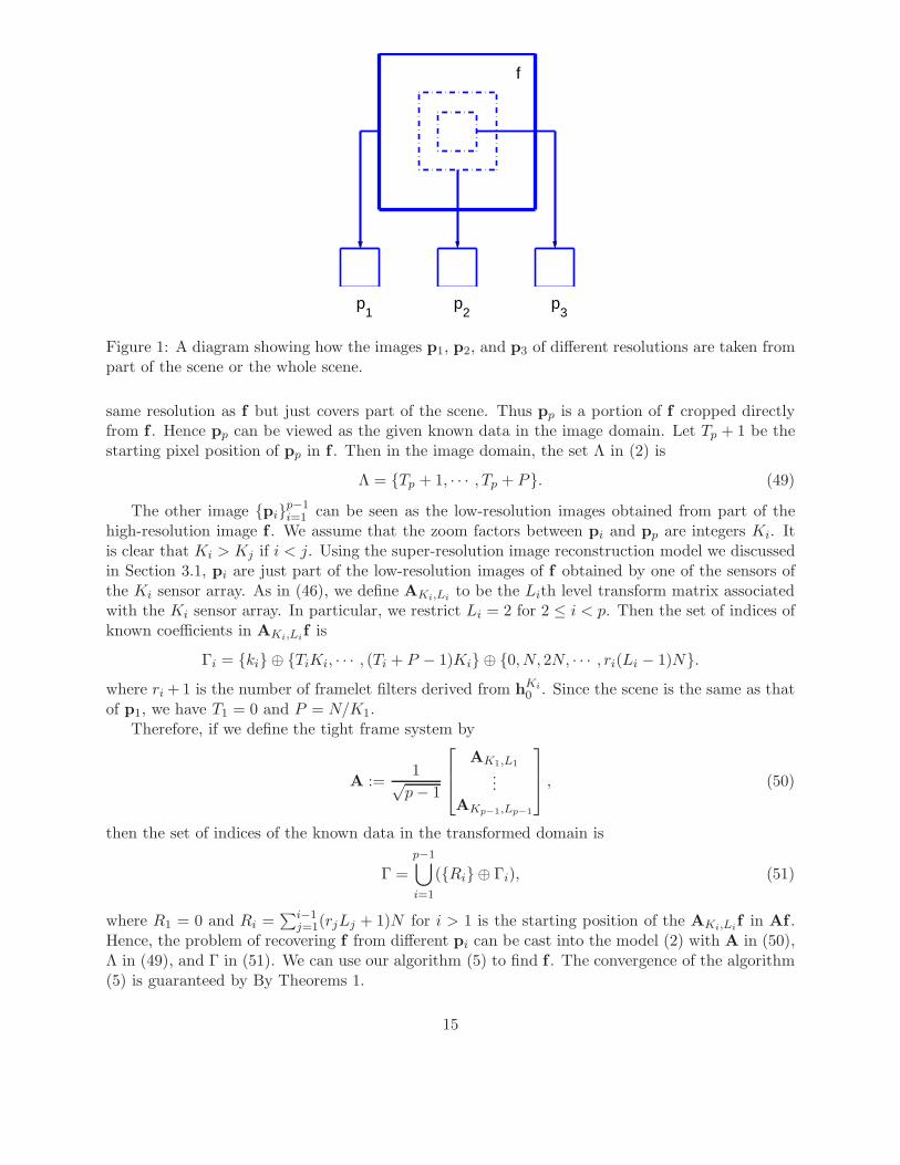
The problem setting is that p images p1,p2, . . . ,pp of a scene or part of it are taken withincreasing zoom ratio, such that all p images have the same number of pixels but with differentresolutions. The image pp has the highest resolution but covers the smallest part of the scene, andp1 is the least zoomed image but covers the entire scene. The problem is to obtain the whole scenecovered by p1 at the resolution same as that of pp. Figure 1 depicts the case where p = 3 and theareas covered by the observed images p1, p2, and p3. Figure 5(a)–(c) give p1, p2, and p3 for realimages “Boat” and “Goldhill”.

We now formulate the problem using the model (2) with appropriate transform matrix A andindex sets Λ and Γ. For simplicity, we only formulate it in 1D. It can easily be extended to 2Dimages. Details can be found in [38]. Let the vectors pip

i=1 be all of length P . Let f ∈ RN be thesolution (i.e. the scene at the highest resolution—same resolution as pp’s.). Note that pp has the

14

p2

p1

p3

f

Figure 1: A diagram showing how the images p1, p2, and p3 of different resolutions are taken frompart of the scene or the whole scene.

same resolution as f but just covers part of the scene. Thus pp is a portion of f cropped directlyfrom f . Hence pp can be viewed as the given known data in the image domain. Let Tp + 1 be thestarting pixel position of pp in f . Then in the image domain, the set Λ in (2) is

Λ = Tp + 1, · · · , Tp + P. (49)

The other image pip−1i=1 can be seen as the low-resolution images obtained from part of the

high-resolution image f . We assume that the zoom factors between pi and pp are integers Ki. Itis clear that Ki > Kj if i < j. Using the super-resolution image reconstruction model we discussedin Section 3.1, pi are just part of the low-resolution images of f obtained by one of the sensors ofthe Ki sensor array. As in (46), we define AKi,Li

to be the Lith level transform matrix associatedwith the Ki sensor array. In particular, we restrict Li = 2 for 2 ≤ i < p. Then the set of indices ofknown coefficients in AKi,Li

f is

Γi = ki ⊕ TiKi, · · · , (Ti + P − 1)Ki ⊕ 0, N, 2N, · · · , ri(Li − 1)N.where ri + 1 is the number of framelet filters derived from h

Ki

0 . Since the scene is the same as thatof p1, we have T1 = 0 and P = N/K1.

Therefore, if we define the tight frame system by

A :=1√

p − 1

AK1,L1

...AKp−1,Lp−1

, (50)

then the set of indices of the known data in the transformed domain is

Γ =

p−1⋃

i=1

(Ri ⊕ Γi), (51)

where R1 = 0 and Ri =∑i−1

j=1(rjLj + 1)N for i > 1 is the starting position of the AKi,Lif in Af .

Hence, the problem of recovering f from different pi can be cast into the model (2) with A in (50),Λ in (49), and Γ in (51). We can use our algorithm (5) to find f . The convergence of the algorithm(5) is guaranteed by By Theorems 1.

15

3.3 Numerical Results

We now illustrate the applicability of our proposed algorithm (5) for the applications presented inthe last two subsections. We use the “Boat” and “Goldhill” images of size 256×256 as the originalimages in our numerical tests. The objective quality of the reconstructed images is evaluated bythe peak signal-to-noise ratio (PSNR) which is defined as

PSNR = 20 log10

(

255√

N

‖f − f (∞)‖2

)

, (52)

with f being the original image, f (∞) the reconstructed image by (5), and N the number of pixelsin f (∞). The initial seed f (0) is chosen as zero. The maximum number of iteration is set to 100 andthe iteration process is stopped when the reconstructed image achieves the highest PSNR value.

We first consider super-resolution image reconstruction with multiple sensors. We used a 4× 4sensor array (i.e. K = 4). In this case, we choose the parameter r = 5 in (46). The six filters h4

i ,i = 0, 1, 2, 3, 4, 5, are

h40 =

1

4

[1

2, 1, 1, 1,

1

2

]

,h41 =

√2

8[1, 0, 0, 0,−1] ,h4

2 =1

4

[

−1

2, 1,−1, , 1,−1

2

]

h43 =

1

4

[1

2, 1, 0,−1,−1

2

]

,h44 =

√2

8[1, 0,−2, 0, 1] ,h4

5 =1

4

[

−1

2, 1, 0,−1,

1

2

]

.

The sum of the absolute values of the elements in h4i , denoted by ci, i = 0, 1, 2, 3, 4, 5, are 1,√

22 , 1, 3

4 ,√

22 , and 3

4 , respectively. The parameter L in (46) is 4. To determine the thresholdingparameters ui in (4), we first compute a threshold β which basically is a scaled version of thethreshold given in [31], that is, β = 1

64σ√

2 log N . The parameter σ is the estimated standarddeviation of the Gaussian noise in the observed image. The factor 1

64 is empirically chosen basedon our experiments. We choose ui = cpβ if the corresponding framelet coefficient yi is produced by

the subblock H(j)p,4

∏j−1ℓ=1 H

(j−ℓ)0,4 in (46), where 1 ≤ i ≤ 5, and 1 ≤ j ≤ L. Figures 3 and 4 show the

reconstructed images when noise at signal-to-noise ratio 30dB is added to the observed images.Next we test our algorithm for super-resolution image reconstruction from different zooms. In

the test, we set p = 3, K1 = 4, and K2 = 2. The image p1 is the lowest-resolution image of thescene f as obtained from a 4 × 4 sensor array. The image p2 is a low-resolution image of part of f

as obtained from a 2 × 2 sensor array. The image p3 is a part of f . The images p1, p2, and p3 allhave the same size and are 1/16 of the size of f . The images and their restored results are displayedin Figure 5.

4 Conclusion

In this paper, we have developed an algorithm for doing inpainting in both image and transformeddomains. The proposed algorithm is motivated by the perfect reconstruction formula of a tightframelet system. This algorithm is further recognized as a proximal forward-backward splittingiteration of a minimization problem with the help of proximal operator and proximal envelop. Byusing the convergence result of PFBS iteration, we have proved the convergence of the algorithm,and obtained the functionals which the limits will minimize. We have illustrated how to apply themethod to super-resolution image reconstruction from different zooms.

16

References

[1] M. Bertalmio, G. Sapiro, V. Caselles, and C. Ballester, Image inpainting, in Pro-ceedings of SIGGRAPH, New Orleans, LA, 2000, pp. 417–424.

[2] M. Bertalmio, L. Vese, G. Sapiro, and S. Osher, Simultaneous structure and textureimage inpainting, IEEE Transactions on Image Processing, 12 (2003), pp. 882–889.

[3] M. Bertero and P. Boccacci, Introduction to inverse problems in imaging, Institute ofPhysics Pub., Bristol, 1998.

[4] M. Bertero, P. Boccacci, F. D. Benedetto, and M. Robberto, Restoration of choppedand nodded images in infrared astronomy, Inverse Problem, 15 (1999), pp. 345–372.

[5] L. Borup, R. Gribonval and M. Nielsen, Bi-framelet systems with few vanishing momentscharacterize Besov spaces, Appl. Comput. Harmon. Anal., 17 (2004), pp. 3–28.

[6] N. Bose and K. Boo, High-resolution image reconstruction with multisensors, InternationalJournal of Imaging Systems and Technology, 9 (1998), pp. 294–304.

[7] J.-F. Cai, R. Chan, L. Shen, and Z. Shen, Restoration of chopped and nodded images byframelets, SIAM Journal on Scientific Computing, 30(3) (2008), pp. 1205–1227.

[8] J.-F. Cai, R. Chan, and Z. Shen, A framelet-based image inpainting algorithm, Appliedand Computational Harmonic Analysis, 24 (2008), pp. 131–149.

[9] J.-F. Cai, R. Chan, and Z. Shen, Simultaneous Cartoon and Texture Inpainting, preprint,2008.

[10] J.-F. Cai, S. Osher, and Z. Shen, Linearized Bregman iterations for compressed sensing,Mathematics of Computations, to appear.

[11] J.-F. Cai, S. Osher, and Z. Shen, Convergence of the linearized Bregman iteration forℓ1-norm minimization, Mathematics of Computations, to appear.

[12] J.-F. Cai, S. Osher, and Z. Shen, Linearized Bregman iterations for frame-based imagedeblurring, SIAM Journal on Imaging Sciences, to appear.

[13] E. J. Candes and D. L. Donoho, New tight frames of curvelets and optimal representationsof objects with piecewise C2 singularities, Comm. Pure Appl. Math., 57 (2004), pp. 219–266.

[14] E. J. Candes, J. Romberg, and T. Tao, Robust uncertainty principles: exact signal re-construction from highly incomplete frequency information, IEEE Trans. Inform. Theory, 52(2006), pp. 489–509.

[15] A. Chai and Z. Shen, “Deconvolution: A wavelet frame approach”, Numer. Math., 106 (2007),pp. 529–587.

[16] R. Chan, T. Chan, L. Shen, and Z. Shen, Wavelet algorithms for high-resolution imagereconstruction, SIAM Journal on Scientific Computing, 24 (2003), pp. 1408–1432.

[17] , Wavelet deblurring algorithms for spatially varying blur from high-resolution image re-construction, Linear Algebra and its Applications, 366 (2003), pp. 139–155.

17

[18] R. Chan, S. D. Riemenschneider, L. Shen, and Z. Shen, High-resolution image recon-struction with displacement errors: A framelet approach, International Journal of ImagingSystems and Technology, 14 (2004), pp. 91–104.

[19] , Tight frame: The efficient way for high-resolution image reconstruction, Applied andComputational Harmonic Analysis, 17 (2004), pp. 91–115.

[20] R. Chan, L. Shen, and Z. Shen, A framelet-based approach for image inpainting, Tech.Report 2005-4, The Chinese University of Hong Kong, Feb. 2005.

[21] R. Chan, Z. Shen, and T. Xia, A framelet algorithm for enchancing video stills, Appliedand Computational Harmonic Analysis, 23 (2007), pp. 153–170.

[22] T. Chan, S.-H. Kang, and J. Shen, Euler’s elastica and curvature-based image inpainting,SIAM Journal on Applied Mathematics, 63 (2002), pp. 564–592.

[23] T. Chan and J. Shen, Mathematical models for local nontexture inpaintings, SIAM J. AppliedMathematics, 62 (2001), pp. 1019–1043.

[24] T. F. Chan, J. Shen, and H.-M. Zhou, Total variation wavelet inpainting, J. Math. ImagingVision, 25 (2006), pp. 107–125.

[25] P. Combettes and V. Wajs, Signal recovery by proximal forward-backward splitting, Mul-tiscale Modeling and Simulation: A SIAM Interdisciplinary Journal, 4 (2005), pp. 1168–1200.

[26] I. Daubechies, Ten Lectures on Wavelets, vol. 61 of CBMS Conference Series in AppliedMathematics, SIAM, Philadelphia, 1992.

[27] I. Daubechies, B. Han, A. Ron, and Z. Shen, Framelets: MRA-based constructions ofwavelet frames, Applied and Computation Harmonic Analysis, 14 (2003), pp. 1–46.

[28] I. Daubechies, G. Teschke, and L. Vese, Iteratively solving linear inverse problems undergeneral convex constraints, Inverse Probl. Imaging, 1 (2007), pp. 29–46.

[29] A. H. Delaney and Y. Bresler, A fast and accurate Fourier algorithm for iterative parallel-beam tomography, IEEE Trans. Image Process., 5 (1996), pp. 740–753.

[30] M. N. Do and M. Vetterli, The contourlet transform: an efficient directional multiresolu-tion image representation, IEEE Transactions on Image Processing, 14 (2005), pp. 2091–2106.

[31] D. Donoho and I. Johnstone, Ideal spatial adaptation by wavelet shrinkage, Biometrika,81 (1994), pp. 425–455.

[32] M. Elad and A. Feuer, Restoration of a single superresolution image from several blurred,noisy and undersampled measured images, IEEE Transactions on Image Processing, 6 (1997),pp. 1646–1658.

[33] M. Elad, P. Milanfar, and R. Rubinstein, Analysis versus synthesis in signal priors,Inverse Problems, 23 (2007), pp. 947–968.

[34] M. Elad, J.-L. Starck, P. Querre, and D. Donoho, Simultaneous cartoon and textureimage inpainting using morphological component analysis (MCA), Applied and ComputationalHarmonic Analysis, 19 (2005).

18

[35] M. Fadili and J.-L. Starck, Sparse representations and bayesian image inpainting, in Proc.SPARS’05, Vol. I, Rennes, France, 2005.

[36] O. G. Guleryuz, Nonlinear approximation based image recovery using adaptive sparse recon-struction and iterated denoising: Part II - adaptive algorithms, IEEE Transaction on ImageProcessing, (2006).

[37] J.-B. Hiriart-Urruty and C. Lemarechal, Convex analysis and minimization algorithms,vol. 305 of Grundlehren der Mathematischen Wissenschaften [Fundamental Principles of Math-ematical Sciences], Springer-Verlag, Berlin, 1993.

[38] M. V. Joshi, S. Chaudhuri, and R. Panuganti, Super-resolution imaging: use of zoomas a cue, Image and Vision Computing, 22 (2004), pp. 1185–1196.

[39] S. Mallat, A Wavelet Tour of Signal Processing, Academic Press, 2nd ed., 1999.

[40] M. K. Ng and N. Bose, Analysis of displacement errors in high-resolution image reconstruc-tion with multisensors, IEEE Transactions on Circuits and Systems—I: Fundamental Theoryand Applications, 49 (2002), pp. 806–813.

[41] M. K. Ng, R. Chan, and W. Tang, A fast algorithm for deblurring models with Neumannboundary conditions, SIAM Journal on Scientific Computing, 21 (2000), pp. 851–866.

[42] A. Ron and Z. Shen, Affine system in L2(Rd): the analysis of the analysis operator, JournalFunc. Anal., 148 (1997), pp. 408–447.

19

Figure 2: Inpainting in image domain for the “Pepper” and “Goldhill” images. Columns (from leftto right) are the observed incomplete image, the recovered image by (5), the recovered image by thesynthesis based approach, and the recovered image by the analysis based approach, respectively.In the first row, the PSNR values of the recovered images (from the second left to the right) are33.82dB, 32.27dB, 33.73dB, respectively. In the second row, the PSNR values of the recoveredimages (from the second left to the right) are 29.81dB, 28.10dB, 29.80dB, respectively.

20

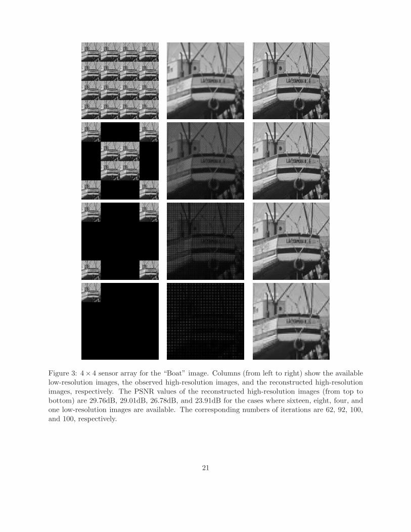
Figure 3: 4× 4 sensor array for the “Boat” image. Columns (from left to right) show the availablelow-resolution images, the observed high-resolution images, and the reconstructed high-resolutionimages, respectively. The PSNR values of the reconstructed high-resolution images (from top tobottom) are 29.76dB, 29.01dB, 26.78dB, and 23.91dB for the cases where sixteen, eight, four, andone low-resolution images are available. The corresponding numbers of iterations are 62, 92, 100,and 100, respectively.

21

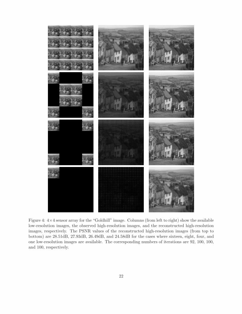
Figure 4: 4×4 sensor array for the “Goldhill” image. Columns (from left to right) show the availablelow-resolution images, the observed high-resolution images, and the reconstructed high-resolutionimages, respectively. The PSNR values of the reconstructed high-resolution images (from top tobottom) are 28.51dB, 27.93dB, 26.49dB, and 24.58dB for the cases where sixteen, eight, four, andone low-resolution images are available. The corresponding numbers of iterations are 92, 100, 100,and 100, respectively.

22

(a) p1 (b) p2 (c) p3 (d) reconstructed image

Figure 5: Reconstructed super-resolution images for images “Boat” (top row) and “Goldhill” (bot-tom row), respectively, from the related low-resolution images p1, p2, p3.

23