Light-weight pixel context encoders for image inpaintingNanne van Noord*

University of Amsterdamn.j.e.vannoord@uva.nl

Eric PostmaTilburg University

e.o.postma@tilburguniversity.edu

ABSTRACTIn this work we propose Pixel Content Encoders (PCE), a light-weight image inpainting model, capable of generating novel contentfor large missing regions in images. Unlike previously presented con-volutional neural network based models, our PCE model has an orderof magnitude fewer trainable parameters. Moreover, by incorporat-ing dilated convolutions we are able to preserve fine grained spatialinformation, achieving state-of-the-art performance on benchmarkdatasets of natural images and paintings. Besides image inpainting,we show that without changing the architecture, PCE can be usedfor image extrapolation, generating novel content beyond existingimage boundaries.

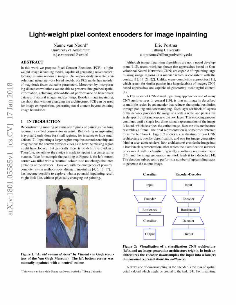
1 INTRODUCTIONReconstructing missing or damaged regions of paintings has longrequired a skilled conservator or artist. Retouching or inpaintingis typically only done for small regions, for instance to hide smalldefects [2]. Inpainting a larger region requires connoisseurship andimagination: the context provides clues as to how the missing regionmight have looked, but generally there is no definitive evidence.Therefore, sometimes the choice is made to inpaint in a conservativemanner. Take for example the painting in Figure 1, the left bottomcorner was filled with a ‘neutral’ colour as to not change the inter-pretation of the artwork. However, with the emergence of powerfulcomputer vision methods specialising in inpainting [4, 6, 12, 17], ithas become possible to explore what a potential inpainting resultmight look like, without physically changing the painting.

Figure 1: “An old woman of Arles” by Vincent van Gogh (cour-tesy of the Van Gogh Museum). The left bottom corner wasmanually inpainted with a ‘neutral’ colour.

*This work was done while Nanne van Noord worked at Tilburg University.

Although image inpainting algorithms are not a novel develop-ment [1, 2], recent work has shown that approaches based on Con-volutional Neural Networks (CNN) are capable of inpainting largemissing image regions in a manner which is consistent with thecontext [12, 17, 21, 22]. Unlike, scene-completion approaches [11],which search for similar patches in a large database of images, CNN-based approaches are capable of generating meaningful content[17].

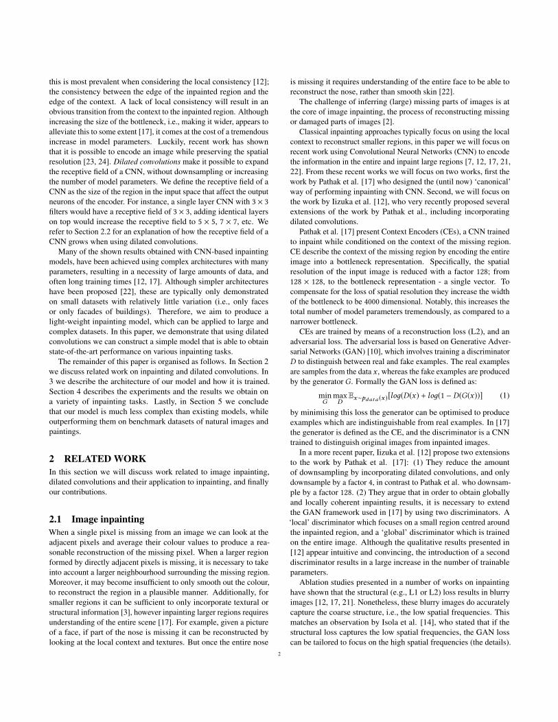
A key aspect of CNN-based inpainting approaches and of manyCNN architectures in general [19], is that an image is describedat multiple scales by an encoder that reduces the spatial resolutionthrough pooling and downsampling. Each layer (or block of layers)of the network processes the image at a certain scale, and passes thisscale-specific information on to the next layer. This encoding processcontinues until a single low dimensional representation of the imageis found, which describes the entire image. Because this architectureresembles a funnel, the final representation is sometimes referredto as the bottleneck. Figure 2 shows a visualisation of two CNNarchitectures; one for classification, and one for image generation(similar to an autoencoder). Both architectures encode the image intoa bottleneck representation, after which the classification networkprocesses it with a classifier, typically a softmax regression layer[16], and the image generation network feeds it to a decoder [14].The decoder subsequently performs a number of upsampling stepsto generate the output image.

Input

Encoder

Bottleneck

Classifier

Output

Classifier

Input

Encoder

Bottleneck

Decoder

Output

Encoder-Decoder

Figure 2: Visualisation of a classification CNN architecture(left), and an image generation architecture (right). In both ar-chitectures the encoder downsamples the input into a low(er)dimensional representation: the bottleneck.

A downside of downsampling in the encoder is the loss of spatialdetail - detail which might be crucial to the task [24]. For inpainting

arX

iv:1

801.

0558

5v1

[cs

.CV

] 1

7 Ja

n 20

18

this is most prevalent when considering the local consistency [12];the consistency between the edge of the inpainted region and theedge of the context. A lack of local consistency will result in anobvious transition from the context to the inpainted region. Althoughincreasing the size of the bottleneck, i.e., making it wider, appears toalleviate this to some extent [17], it comes at the cost of a tremendousincrease in model parameters. Luckily, recent work has shownthat it is possible to encode an image while preserving the spatialresolution [23, 24]. Dilated convolutions make it possible to expandthe receptive field of a CNN, without downsampling or increasingthe number of model parameters. We define the receptive field of aCNN as the size of the region in the input space that affect the outputneurons of the encoder. For instance, a single layer CNN with 3 × 3filters would have a receptive field of 3 × 3, adding identical layerson top would increase the receptive field to 5 × 5, 7 × 7, etc. Werefer to Section 2.2 for an explanation of how the receptive field of aCNN grows when using dilated convolutions.

Many of the shown results obtained with CNN-based inpaintingmodels, have been achieved using complex architectures with manyparameters, resulting in a necessity of large amounts of data, andoften long training times [12, 17]. Although simpler architectureshave been proposed [22], these are typically only demonstratedon small datasets with relatively little variation (i.e., only facesor only facades of buildings). Therefore, we aim to produce alight-weight inpainting model, which can be applied to large andcomplex datasets. In this paper, we demonstrate that using dilatedconvolutions we can construct a simple model that is able to obtainstate-of-the-art performance on various inpainting tasks.

The remainder of this paper is organised as follows. In Section 2we discuss related work on inpainting and dilated convolutions. In3 we describe the architecture of our model and how it is trained.Section 4 describes the experiments and the results we obtain ona variety of inpainting tasks. Lastly, in Section 5 we concludethat our model is much less complex than existing models, whileoutperforming them on benchmark datasets of natural images andpaintings.

2 RELATED WORKIn this section we will discuss work related to image inpainting,dilated convolutions and their application to inpainting, and finallyour contributions.

2.1 Image inpaintingWhen a single pixel is missing from an image we can look at theadjacent pixels and average their colour values to produce a rea-sonable reconstruction of the missing pixel. When a larger regionformed by directly adjacent pixels is missing, it is necessary to takeinto account a larger neighbourhood surrounding the missing region.Moreover, it may become insufficient to only smooth out the colour,to reconstruct the region in a plausible manner. Additionally, forsmaller regions it can be sufficient to only incorporate textural orstructural information [3], however inpainting larger regions requiresunderstanding of the entire scene [17]. For example, given a pictureof a face, if part of the nose is missing it can be reconstructed bylooking at the local context and textures. But once the entire nose

is missing it requires understanding of the entire face to be able toreconstruct the nose, rather than smooth skin [22].

The challenge of inferring (large) missing parts of images is atthe core of image inpainting, the process of reconstructing missingor damaged parts of images [2].

Classical inpainting approaches typically focus on using the localcontext to reconstruct smaller regions, in this paper we will focus onrecent work using Convolutional Neural Networks (CNN) to encodethe information in the entire and inpaint large regions [7, 12, 17, 21,22]. From these recent works we will focus on two works, first thework by Pathak et al. [17] who designed the (until now) ‘canonical’way of performing inpainting with CNN. Second, we will focus onthe work by Iizuka et al. [12], who very recently proposed severalextensions of the work by Pathak et al., including incorporatingdilated convolutions.

Pathak et al. [17] present Context Encoders (CEs), a CNN trainedto inpaint while conditioned on the context of the missing region.CE describe the context of the missing region by encoding the entireimage into a bottleneck representation. Specifically, the spatialresolution of the input image is reduced with a factor 128; from128 × 128, to the bottleneck representation - a single vector. Tocompensate for the loss of spatial resolution they increase the widthof the bottleneck to be 4000 dimensional. Notably, this increases thetotal number of model parameters tremendously, as compared to anarrower bottleneck.

CEs are trained by means of a reconstruction loss (L2), and anadversarial loss. The adversarial loss is based on Generative Adver-sarial Networks (GAN) [10], which involves training a discriminatorD to distinguish between real and fake examples. The real examplesare samples from the data x , whereas the fake examples are producedby the generator G. Formally the GAN loss is defined as:

minG

maxDEx∼pdata (x )[loд(D(x) + loд(1 − D(G(x))] (1)

by minimising this loss the generator can be optimised to produceexamples which are indistinguishable from real examples. In [17]the generator is defined as the CE, and the discriminator is a CNNtrained to distinguish original images from inpainted images.

In a more recent paper, Iizuka et al. [12] propose two extensionsto the work by Pathak et al. [17]: (1) They reduce the amountof downsampling by incorporating dilated convolutions, and onlydownsample by a factor 4, in contrast to Pathak et al. who downsam-ple by a factor 128. (2) They argue that in order to obtain globallyand locally coherent inpainting results, it is necessary to extendthe GAN framework used in [17] by using two discriminators. A‘local’ discriminator which focuses on a small region centred aroundthe inpainted region, and a ‘global’ discriminator which is trainedon the entire image. Although the qualitative results presented in[12] appear intuitive and convincing, the introduction of a seconddiscriminator results in a large increase in the number of trainableparameters.

Ablation studies presented in a number of works on inpaintinghave shown that the structural (e.g., L1 or L2) loss results in blurryimages [12, 17, 21]. Nonetheless, these blurry images do accuratelycapture the coarse structure, i.e., the low spatial frequencies. Thismatches an observation by Isola et al. [14], who stated that if thestructural loss captures the low spatial frequencies, the GAN losscan be tailored to focus on the high spatial frequencies (the details).

2

Specifically, Isola et al. introduced PatchGAN, a GAN which fo-cuses on the structure in local patches, relying on the structural lossto ensure correctness of the global structure. PatchGAN, produces ajudgement for N × N patches, where N can be much smaller thanthe whole image. When N is smaller than the image, PatchGAN isapplied convolutionally and the judgements are averaged to producea single outcome.

Because the PatchGAN operates on patches it has to downsampleless, reducing the number of parameters as compared to typical GANarchitectures, this fits well with our aim to produce a light-weightinpainting model. Therefore, in our work we choose to use thePatchGAN for all experiments.

Before turning to explanation of the complete model in section 3,we first describe dilated convolutions in more detail.

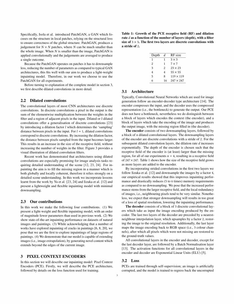
2.2 Dilated convolutionsThe convolutional layers of most CNN architectures use discreteconvolutions. In discrete convolutions a pixel in the output is thesum of the elementwise multiplication between the weights in thefilter and a region of adjacent pixels in the input. Dilated or l-dilatedconvolutions offer a generalisation of discrete convolutions [23]by introducing a dilation factor l which determines the ‘sampling’distance between pixels in the input. For l = 1, dilated convolutionscorrespond to discrete convolutions. By increasing the dilation factor,the distance between pixels sampled from the input becomes larger.This results in an increase in the size of the receptive field, withoutincreasing the number of weights in the filter. Figure 3 provides avisual illustration of dilated convolution filters.

Recent work has demonstrated that architectures using dilatedconvolutions are especially promising for image analysis tasks re-quiring detailed understanding of the scene [12, 23, 24]. For in-painting the aim is to fill the missing region in a manner which isboth globally and locally coherent, therefore it relies strongly on adetailed scene understanding. In this work we incorporate lessonslearnt from the work by Yu et al. [23, 24] and Iizuka et al. [12] andpresent a lightweight and flexible inpainting model with minimaldownsampling.

2.3 Our contributionsIn this work we make the following four contributions. (1) Wepresent a light-weight and flexible inpainting model, with an orderof magnitude fewer parameters than used in previous work. (2) Weshow state-of-the-art inpainting performance on datasets of naturalimages and paintings. (3) While acknowledging that a number ofworks have explored inpainting of cracks in paintings [6, 8, 20], wepose that we are the first to explore inpaintings of large regions ofpaintings. (4) We demonstrate that our model is capable of extendingimages (i.e., image extrapolation), by generating novel content whichextends beyond the edges of the current image.

3 PIXEL CONTEXT ENCODERSIn this section we will describe our inpainting model: Pixel ContextEncoders (PCE). Firstly, we will describe the PCE architecture,followed by details on the loss function used for training.

Table 1: Growth of the PCE receptive field (RF) and dilationrate d as a function of the number of layers (depth), with a filtersize of 3 × 3. The first two layers are discrete convolutions witha stride of 2.

Depth d RF size1 1 3 × 32 1 7 × 73 2 23 × 234 4 55 × 555 8 119 × 1196 16 247 × 247

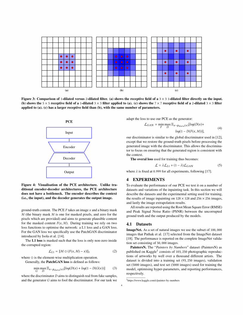
3.1 ArchitectureTypically, Convolutional Neural Networks which are used for imagegeneration follow an encoder-decoder type architecture [14]. Theencoder compresses the input, and the decoder uses the compressedrepresentation (i.e., the bottleneck) to generate the output. Our PCEdoes not have a bottleneck, nevertheless we do distinguish betweena block of layers which encodes the context (the encoder), and ablock of layers which take the encoding of the image and producesthe output image, with the missing region filled in (the decoder).

The encoder consists of two downsampling layers, followed bya block of n dilated convolutional layers. The downsampling layersof the encoder are discrete convolutions with a stride of 2. For thesubsequent dilated convolution layers, the dilation rate d increasesexponentially. The depth of the encoder is chosen such that thereceptive field of the encoder is (at least) larger than the missingregion, for all of our experiments n = 4, resulting in a receptive fieldof 247× 247. Table 1 shows how the size of the receptive field growsas more layers are added to the encoder.

By incorporating strided convolutions in the first two layers wefollow Iizuka et al. [12] and downsample the images by a factor 4,our empirical results showed that this improves inpainting perfor-mance and drastically reduces (5 to 6 times) memory requirementsas compared to no downsampling. We pose that the increased perfor-mance stems from the larger receptive field, and the local redundancyof images, i.e., neighbouring pixels tend to be very similar. Nonethe-less, we expect that stronger downsampling will results in too greatof a loss of spatial resolution, lowering the inpainting performance.

The decoder consists of a block of 3 discrete convolutional lay-ers which take as input the image encoding produced by the en-coder. The last two layers of the decoder are preceded by a nearest-neighbour interpolation layer, which upsamples by a factor 2, restor-ing the image to the original resolution. Additionally, the last layermaps the image encoding back to RGB space (i.e., 3 colour chan-nels), after which all pixels which were not missing are restored tothe ground-truth values.

All convolutional layers in the encoder and decoder, except forthe last decoder layer, are followed by a Batch Normalisation layer[13]. The activation functions for all convolutional layers in theencoder and decoder are Exponential Linear Units (ELU) [5].

3.2 LossPCEs are trained through self-supervision; an image is artificiallycorrupted, and the model is trained to regress back the uncorrupted

3

(a) (b) (c)

Figure 3: Comparison of 1-dilated versus 2-dilated filter. (a) shows the receptive field of a 3 × 3 1-dilated filter directly on the input.(b) shows the 5 × 5 receptive field of a 1-dilated 3 × 3 filter applied to (a). (c) shows the 7 × 7 receptive field of a 2-dilated 3 × 3 filterapplied to (a). (c) has a larger receptive field than (b), with the same number of parameters.

Input

Encoder

Decoder

Output

PCE

Figure 4: Visualisation of the PCE architecture. Unlike tra-ditional encoder-decoder architectures, the PCE architecturedoes not have a bottleneck. The encoder describes the context(i.e., the input), and the decoder generates the output image.

ground-truth content. The PCE F takes an image x and a binary maskM (the binary mask M is one for masked pixels, and zero for thepixels which are provided) and aims to generate plausible contentfor the masked content F (x ,M). During training we rely on twoloss functions to optimise the network: a L1 loss and a GAN loss.For the GAN loss we specifically use the PatchGAN discriminatorintroduced by Isola et al. [14].

The L1 loss is masked such that the loss is only non-zero insidethe corrupted region:

LL1 = ‖M � (F (x ,M) − x)‖1 (2)

where � is the element-wise multiplication operation.Generally, the PatchGAN loss is defined as follows:

minG

maxDEx∼pdata (x )[loд(D(x) + loд(1 − D(G(x))] (3)

where the discriminator D aims to distinguish real from fake samples,and the generator G aims to fool the discriminator. For our task we

adapt the loss to use our PCE as the generator:

LGAN = minF

maxDEx∼pdata (x )[loд(D(x)+

loд(1 − D(F (x ,M))],(4)

our discriminator is similar to the global discriminator used in [12],except that we restore the ground-truth pixels before processing thegenerated image with the discriminator. This allows the discrimina-tor to focus on ensuring that the generated region is consistent withthe context.

The overal loss used for training thus becomes:

L = λLL1 + (1 − λ)LGAN (5)

where λ is fixed at 0.999 for all experiments, following [17].

4 EXPERIMENTSTo evaluate the performance of our PCE we test it on a number ofdatasets and variations of the inpainting task. In this section we willdescribe the datasets and the experimental setting used for training,the results of image inpainting on 128 × 128 and 256 × 256 images,and lastly the image extrapolation results.

All results are reported using the Root Mean Square Error (RMSE)and Peak Signal Noise Ratio (PSNR) between the uncorruptedground truth and the output produced by the models.

4.1 DatasetsImageNet. As a set of natural images we use the subset of 100, 000images that Pathak et al. [17] selected from the ImageNet dataset[18]. The performance is reported on the complete ImageNet valida-tion set consisting of 50, 000 images.

PaintersN. The “Painters by Numbers” dataset (PaintersN) aspublished on Kaggle1 consists of 103, 250 photographic reproduc-tions of artworks by well over a thousand different artists. Thedataset is divided into a training set (93, 250 images), validationset (5000 images), and test set (5000 images) used for training themodel, optimising hyper-parameters, and reporting performances,respectively.

1https://www.kaggle.com/c/painter-by-numbers

4

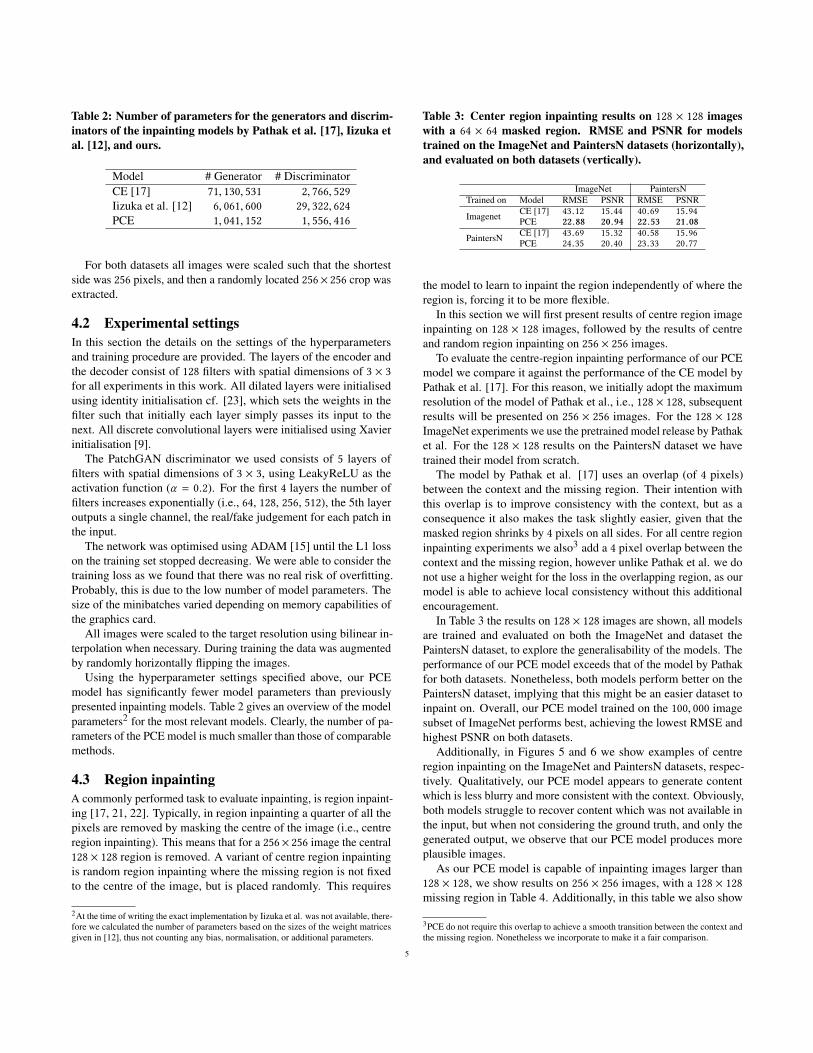
Table 2: Number of parameters for the generators and discrim-inators of the inpainting models by Pathak et al. [17], Iizuka etal. [12], and ours.

Model # Generator # DiscriminatorCE [17] 71, 130, 531 2, 766, 529Iizuka et al. [12] 6, 061, 600 29, 322, 624PCE 1, 041, 152 1, 556, 416

For both datasets all images were scaled such that the shortestside was 256 pixels, and then a randomly located 256× 256 crop wasextracted.

4.2 Experimental settingsIn this section the details on the settings of the hyperparametersand training procedure are provided. The layers of the encoder andthe decoder consist of 128 filters with spatial dimensions of 3 × 3for all experiments in this work. All dilated layers were initialisedusing identity initialisation cf. [23], which sets the weights in thefilter such that initially each layer simply passes its input to thenext. All discrete convolutional layers were initialised using Xavierinitialisation [9].

The PatchGAN discriminator we used consists of 5 layers offilters with spatial dimensions of 3 × 3, using LeakyReLU as theactivation function (α = 0.2). For the first 4 layers the number offilters increases exponentially (i.e., 64, 128, 256, 512), the 5th layeroutputs a single channel, the real/fake judgement for each patch inthe input.

The network was optimised using ADAM [15] until the L1 losson the training set stopped decreasing. We were able to consider thetraining loss as we found that there was no real risk of overfitting.Probably, this is due to the low number of model parameters. Thesize of the minibatches varied depending on memory capabilities ofthe graphics card.

All images were scaled to the target resolution using bilinear in-terpolation when necessary. During training the data was augmentedby randomly horizontally flipping the images.

Using the hyperparameter settings specified above, our PCEmodel has significantly fewer model parameters than previouslypresented inpainting models. Table 2 gives an overview of the modelparameters2 for the most relevant models. Clearly, the number of pa-rameters of the PCE model is much smaller than those of comparablemethods.

4.3 Region inpaintingA commonly performed task to evaluate inpainting, is region inpaint-ing [17, 21, 22]. Typically, in region inpainting a quarter of all thepixels are removed by masking the centre of the image (i.e., centreregion inpainting). This means that for a 256× 256 image the central128 × 128 region is removed. A variant of centre region inpaintingis random region inpainting where the missing region is not fixedto the centre of the image, but is placed randomly. This requires

2At the time of writing the exact implementation by Iizuka et al. was not available, there-fore we calculated the number of parameters based on the sizes of the weight matricesgiven in [12], thus not counting any bias, normalisation, or additional parameters.

Table 3: Center region inpainting results on 128 × 128 imageswith a 64 × 64 masked region. RMSE and PSNR for modelstrained on the ImageNet and PaintersN datasets (horizontally),and evaluated on both datasets (vertically).

ImageNet PaintersNTrained on Model RMSE PSNR RMSE PSNR

Imagenet CE [17] 43.12 15.44 40.69 15.94PCE 22.88 20.94 22.53 21.08

PaintersN CE [17] 43.69 15.32 40.58 15.96PCE 24.35 20.40 23.33 20.77

the model to learn to inpaint the region independently of where theregion is, forcing it to be more flexible.

In this section we will first present results of centre region imageinpainting on 128 × 128 images, followed by the results of centreand random region inpainting on 256 × 256 images.

To evaluate the centre-region inpainting performance of our PCEmodel we compare it against the performance of the CE model byPathak et al. [17]. For this reason, we initially adopt the maximumresolution of the model of Pathak et al., i.e., 128 × 128, subsequentresults will be presented on 256 × 256 images. For the 128 × 128ImageNet experiments we use the pretrained model release by Pathaket al. For the 128 × 128 results on the PaintersN dataset we havetrained their model from scratch.

The model by Pathak et al. [17] uses an overlap (of 4 pixels)between the context and the missing region. Their intention withthis overlap is to improve consistency with the context, but as aconsequence it also makes the task slightly easier, given that themasked region shrinks by 4 pixels on all sides. For all centre regioninpainting experiments we also3 add a 4 pixel overlap between thecontext and the missing region, however unlike Pathak et al. we donot use a higher weight for the loss in the overlapping region, as ourmodel is able to achieve local consistency without this additionalencouragement.

In Table 3 the results on 128 × 128 images are shown, all modelsare trained and evaluated on both the ImageNet and dataset thePaintersN dataset, to explore the generalisability of the models. Theperformance of our PCE model exceeds that of the model by Pathakfor both datasets. Nonetheless, both models perform better on thePaintersN dataset, implying that this might be an easier dataset toinpaint on. Overall, our PCE model trained on the 100, 000 imagesubset of ImageNet performs best, achieving the lowest RMSE andhighest PSNR on both datasets.

Additionally, in Figures 5 and 6 we show examples of centreregion inpainting on the ImageNet and PaintersN datasets, respec-tively. Qualitatively, our PCE model appears to generate contentwhich is less blurry and more consistent with the context. Obviously,both models struggle to recover content which was not available inthe input, but when not considering the ground truth, and only thegenerated output, we observe that our PCE model produces moreplausible images.

As our PCE model is capable of inpainting images larger than128 × 128, we show results on 256 × 256 images, with a 128 × 128missing region in Table 4. Additionally, in this table we also show

3PCE do not require this overlap to achieve a smooth transition between the context andthe missing region. Nonetheless we incorporate to make it a fair comparison.

5

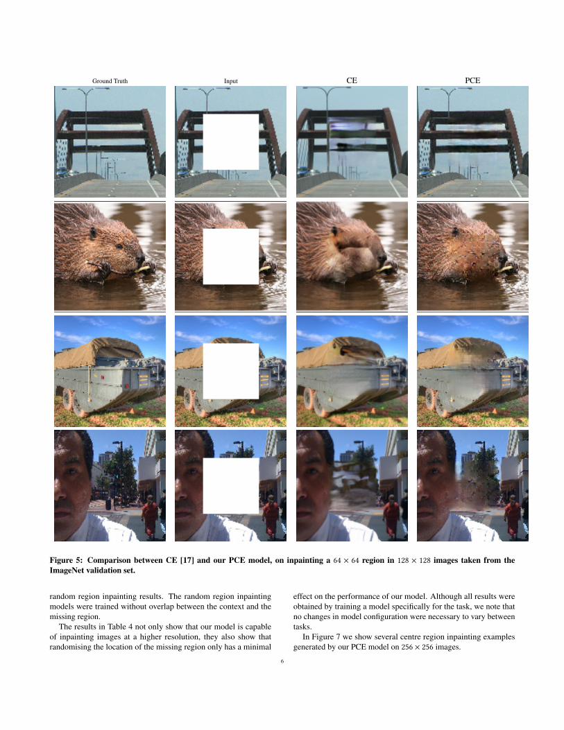
Ground Truth Input CE PCE

Figure 5: Comparison between CE [17] and our PCE model, on inpainting a 64 × 64 region in 128 × 128 images taken from theImageNet validation set.

random region inpainting results. The random region inpaintingmodels were trained without overlap between the context and themissing region.

The results in Table 4 not only show that our model is capableof inpainting images at a higher resolution, they also show thatrandomising the location of the missing region only has a minimal

effect on the performance of our model. Although all results wereobtained by training a model specifically for the task, we note thatno changes in model configuration were necessary to vary betweentasks.

In Figure 7 we show several centre region inpainting examplesgenerated by our PCE model on 256 × 256 images.

6

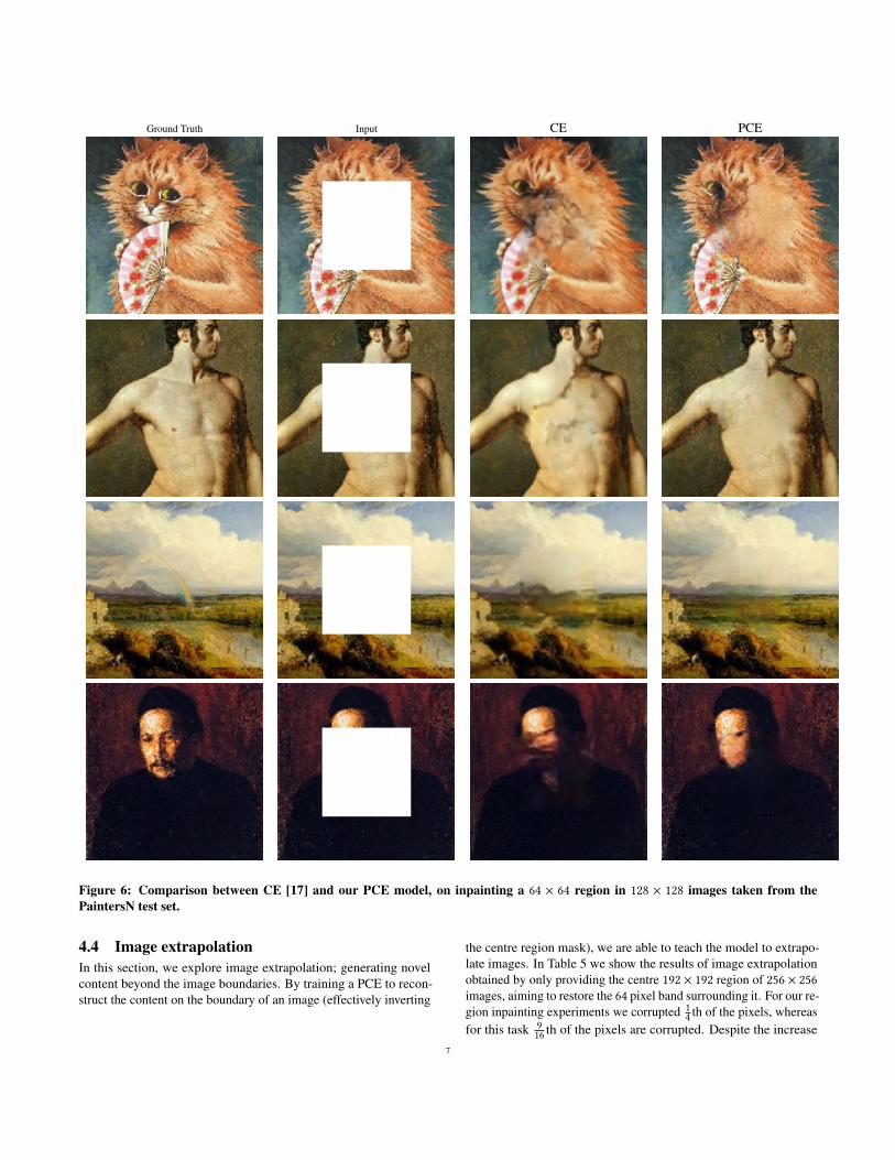
Ground Truth Input CE PCE

Figure 6: Comparison between CE [17] and our PCE model, on inpainting a 64 × 64 region in 128 × 128 images taken from thePaintersN test set.

4.4 Image extrapolationIn this section, we explore image extrapolation; generating novelcontent beyond the image boundaries. By training a PCE to recon-struct the content on the boundary of an image (effectively inverting

the centre region mask), we are able to teach the model to extrapo-late images. In Table 5 we show the results of image extrapolationobtained by only providing the centre 192 × 192 region of 256 × 256images, aiming to restore the 64 pixel band surrounding it. For our re-gion inpainting experiments we corrupted 1

4 th of the pixels, whereasfor this task 9

16 th of the pixels are corrupted. Despite the increase7

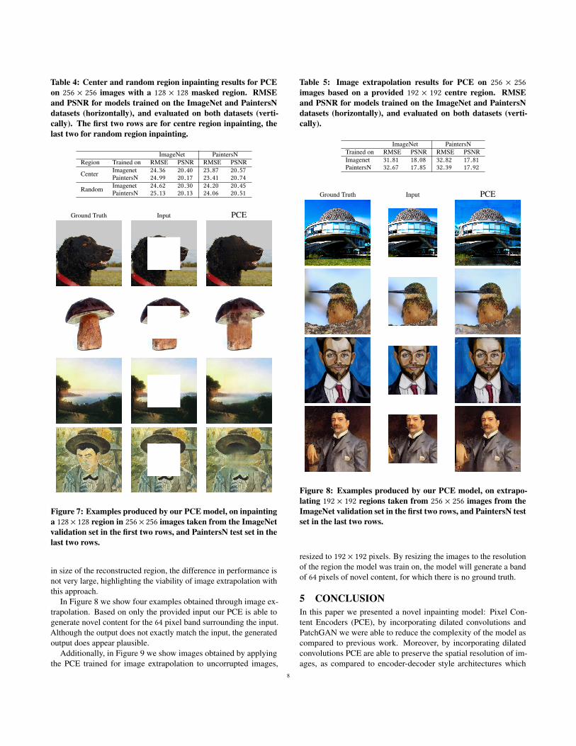
Table 4: Center and random region inpainting results for PCEon 256 × 256 images with a 128 × 128 masked region. RMSEand PSNR for models trained on the ImageNet and PaintersNdatasets (horizontally), and evaluated on both datasets (verti-cally). The first two rows are for centre region inpainting, thelast two for random region inpainting.

ImageNet PaintersNRegion Trained on RMSE PSNR RMSE PSNR

Center Imagenet 24.36 20.40 23.87 20.57PaintersN 24.99 20.17 23.41 20.74

Random Imagenet 24.62 20.30 24.20 20.45PaintersN 25.13 20.13 24.06 20.51

Ground Truth Input PCE

Figure 7: Examples produced by our PCE model, on inpaintinga 128 × 128 region in 256 × 256 images taken from the ImageNetvalidation set in the first two rows, and PaintersN test set in thelast two rows.

in size of the reconstructed region, the difference in performance isnot very large, highlighting the viability of image extrapolation withthis approach.

In Figure 8 we show four examples obtained through image ex-trapolation. Based on only the provided input our PCE is able togenerate novel content for the 64 pixel band surrounding the input.Although the output does not exactly match the input, the generatedoutput does appear plausible.

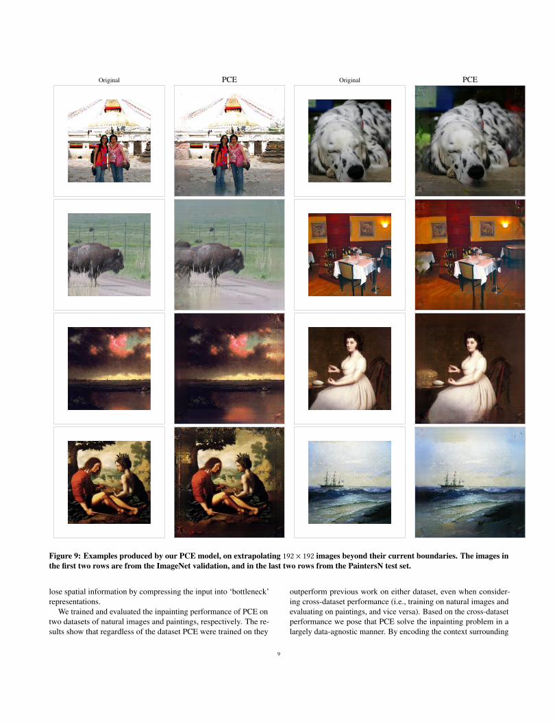
Additionally, in Figure 9 we show images obtained by applyingthe PCE trained for image extrapolation to uncorrupted images,

Table 5: Image extrapolation results for PCE on 256 × 256images based on a provided 192 × 192 centre region. RMSEand PSNR for models trained on the ImageNet and PaintersNdatasets (horizontally), and evaluated on both datasets (verti-cally).

ImageNet PaintersNTrained on RMSE PSNR RMSE PSNRImagenet 31.81 18.08 32.82 17.81PaintersN 32.67 17.85 32.39 17.92

Ground Truth Input PCE

Figure 8: Examples produced by our PCE model, on extrapo-lating 192 × 192 regions taken from 256 × 256 images from theImageNet validation set in the first two rows, and PaintersN testset in the last two rows.

resized to 192 × 192 pixels. By resizing the images to the resolutionof the region the model was train on, the model will generate a bandof 64 pixels of novel content, for which there is no ground truth.

5 CONCLUSIONIn this paper we presented a novel inpainting model: Pixel Con-tent Encoders (PCE), by incorporating dilated convolutions andPatchGAN we were able to reduce the complexity of the model ascompared to previous work. Moreover, by incorporating dilatedconvolutions PCE are able to preserve the spatial resolution of im-ages, as compared to encoder-decoder style architectures which

8

Original PCE Original PCE

Figure 9: Examples produced by our PCE model, on extrapolating 192 × 192 images beyond their current boundaries. The images inthe first two rows are from the ImageNet validation, and in the last two rows from the PaintersN test set.

lose spatial information by compressing the input into ‘bottleneck’representations.

We trained and evaluated the inpainting performance of PCE ontwo datasets of natural images and paintings, respectively. The re-sults show that regardless of the dataset PCE were trained on they

outperform previous work on either dataset, even when consider-ing cross-dataset performance (i.e., training on natural images andevaluating on paintings, and vice versa). Based on the cross-datasetperformance we pose that PCE solve the inpainting problem in alargely data-agnostic manner. By encoding the context surrounding

9

the missing region PCE are able to generate plausible content forthe missing region in a manner that is coherent with the context.

The approach presented in this paper does not explicitly take intoaccount the artist’s style. However, we would argue that the contextreflects the artist’s style, and that generated content coherent withthe context is therefore also reflects the artist’s style. Future researchon explicitly incorporating the artist’s style is necessary to determinewhether it is beneficial for inpainting on artworks to encode theartist’s style in addition to the context.

We conclude that PCE offer a promising avenue for image in-painting and image extrapolation. With an order of magnitude fewermodel parameters than previous inpainting models, PCE obtain state-of-the-art performance on benchmark datasets of natural images andpaintings. Moreover, due to the flexibility of the PCE architecture itcan be used for other image generation tasks, such as image extrapo-lation. We demonstrate the image extrapolation capabilities of ourmodel by restoring boundary content of images, and by generatingnovel content beyond the existing boundaries.

REFERENCES[1] Connelly Barnes, Eli Shechtman, Adam Finkelstein, Dan B Goldman, and Adobe

Systems. 2009. PatchMatch: A Randomized Correspondence Algorithm forStructural Image Editing. ACM Transactions on Graphics 28, 3 (2009), 24–1.

[2] Marcelo Bertalmio, Guillermo Sapiro, Vicent Caselles, Coloma Ballester, Es-cola Superior Politecnica, and Universitat Pompeu Fabra. 2000. Image Inpainting.ACM SIGGRAPH (2000).

[3] Marcelo Bertalmio, Luminita Vese, Guillermo Sapiro, and Stanley Osher. 2003.Simultaneous structure and texture image inpainting. IEEE Transactions on ImageProcessing 12, 8 (2003), 882–889.

[4] R H Chan, J F Yang, and X M Yuan. 2011. Alternating direction method forimage inpainting in wavelet domain. SIAM J. Imaging Sci 4, 3 (2011), 807–826.

[5] Djork-Arne Clevert, Thomas Unterthiner, and Sepp Hochreiter. 2016. Fast andAccurate Deep Network Learning by Exponential Linear Units (ELUs). arXivpreprint (2016), 1–14. arXiv:arXiv:1511.07289v5

[6] B. Cornelis, T. Ruzic, E. Gezels, a. Dooms, a. Pizurica, L. Platisa, J. Cornelis, M.Martens, M. De Mey, and I. Daubechies. 2013. Crack detection and inpaintingfor virtual restoration of paintings: The case of the Ghent Altarpiece. SignalProcessing 93, 3 (mar 2013), 605–619. https://doi.org/10.1016/j.sigpro.2012.07.022

[7] Ruohan Gao and Kristen Grauman. 2017. From One-Trick Ponies to All-Rounders: On-Demand Learning for Image Restoration. arXiv preprint (2017).arXiv:arXiv:1612.01380v2

[8] Ioannis Giakoumis, Nikos Nikolaidis, and Ioannis Pitas. 2006. Digital image pro-cessing techniques for the detection and removal of cracks in digitized paintings.IEEE Transactions on Image Processing 15 (2006), 178–188.

[9] Xavier Glorot and Yoshua Bengio. 2010. Understanding the difficulty of train-ing deep feedforward neural networks. Proceedings of the 13th InternationalConference on Artificial Intelligence and Statistics (AISTATS) 9 (2010), 249–256.https://doi.org/10.1.1.207.2059

[10] Ian J Goodfellow, Jean Pouget-abadie, Mehdi Mirza, Bing Xu, David Warde-farley, Sherjil Ozair, Aaron Courville, and Yoshua Bengio. 2014. GenerativeAdversarial Nets. In NIPS. 2672–2680. arXiv:arXiv:1406.2661v1

[11] James Hays and Alexei A Efros. 2007. Scene Completion Using Millions ofPhotographs. ACM Transactions on Graphics 26, 3 (2007), 1–8. https://doi.org/10.1145/1239451.1239455

[12] Satoshi Iizuka, Edgar Simo-serra, and Hiroshi Ishikawa. 2017. Globally andLocally Consistent Image Completion. ACM Transactions on Graphics (Proc. ofSIGGRAPH 2017) 36, 4 (2017), 107:1—-107:14.

[13] Sergey Ioffe and Christian Szegedy. 2015. Batch Normalization: AcceleratingDeep Network Training by Reducing Internal Covariate Shift. In ICML. JMLR,448–456. arXiv:1502.03167 http://arxiv.org/abs/1502.03167

[14] Phillip Isola, Jun-yan Zhu, Tinghui Zhou, and Alexei A Efros. 2016. Image-to-Image Translation with Conditional Adversarial Networks. arXiv preprint (2016).arXiv:1611.07004

[15] Diederik P. Kingma and Jimmy Lei Ba. 2015. Adam: a Method for StochasticOptimization. In International Conference on Learning Representations. 1–13.arXiv:arXiv:1412.6980v5

[16] Alex Krizhevsky, I Sutskever, and GE Hinton. 2012. ImageNet Classifica-tion with Deep Convolutional Neural Networks.. In Advances in Neural In-formation Processing Systems 25. 1097–1105. https://papers.nips.cc/paper/

4824-imagenet-classification-with-deep-convolutional-neural-networks.pdf[17] Deepak Pathak, Jeff Donahue, Trevor Darrell, and Alexei A Efros. 2016. Context

Encoders: Feature Learning by Inpainting. In CVPR. arXiv:arXiv:1604.07379v1[18] Olga Russakovsky, Jia Deng, Hao Su, Jonathan Krause, Sanjeev Satheesh, Sean

Ma, Zhiheng Huang, Andrej Karpathy, Aditya Khosla, Michael Bernstein, Alexan-der C. Berg, and Li Fei-Fei. 2014. ImageNet Large Scale Visual Recogni-tion Challenge. Arxiv (2014), 37. https://doi.org/10.1007/s11263-015-0816-yarXiv:1409.0575

[19] Pierre Sermanet and Yann Lecun. 2011. Traffic sign recognition with multi-scaleconvolutional networks. Proceedings of the International Joint Conference onNeural Networks SEPTEMBER 2011 (2011), 2809–2813. https://doi.org/10.1109/IJCNN.2011.6033589

[20] V Solanki and A R Mahajan. 2009. Digital Image Processing Approach forInspecting and Interpolating Cracks in Digitized Pictures. International Journalof Recent Trends in Engineering (IJRTE) 1 (2009), 97–99.

[21] Chao Yang, Xin Lu, Zhe Lin, Eli Shechtman, Oliver Wang, and Hao Li. 2017.High-Resolution Image Inpainting using Multi-Scale Neural Patch Synthesis.arXiv preprint (2017). arXiv:1611.09969

[22] Raymond Yeh, Chen Chen, Teck Yian Lim, Mark Hasegawa-johnson, and Minh NDo. 2016. Semantic Image Inpainting with Perceptual and Contextual Losses.arXiv preprint (2016). arXiv:arXiv:1607.07539v2

[23] Fisher Yu and Vladlen Koltun. 2016. Multi-Scale Context Aggregation by Di-lated Convolutions. In Iclr. 1–9. https://doi.org/10.16373/j.cnki.ahr.150049arXiv:1511.07122

[24] Fisher Yu, Vladlen Koltun, Intel Labs, and Thomas Funkhouser. 2017. DilatedResidual Networks. arXiv preprint (2017). arXiv:arXiv:1705.09914v1

10