1

1

Accepted for publication in the Journal of Materials Engineering and Performance, July 2011- in print December 2011

Simulation of Viscoplastic Deformation of Low Carbon Steel-

Structures at Elevated Temperatures

Y. Sun, K. Maciejewski, and H. Ghonem

Mechanics of Materials Research Laboratory

Department of Mechanical Engineering and Applied Mechanics University of Rhode Island, Kingston, R.I. 02881, U.S.A

________________________________________________________________________ Abstract The deformation response of a low carbon structural steel subjected to high temperature simulating fire conditions is generated using a viscoplastic material constitutive model which acknowledges the evolution of the material hardening parameters during the loading history. The material model is implemented in an ABAQUS subroutine (UMAT) which requires the determination of the material constants as a function of temperature. Both the temperature dependency and strain-rate sensitivity of the material parameters have been examined by analysis of a single steel beam and a steel-framed structure subjected to temperatures ranging from 300 oC -700 oC . Sequentially coupled thermal-stress analysis is applied to a structure under simulated fire condition. Results of this analysis show that above a transitional temperature, the deformation of the steel is strain-rate dependent. The combined effect of heat flux and loading rate on the complex deformation of a two story steel structure is examined and the significance of employing a viscoplastic material model is discussed. Keywords: Internal State Variables, Viscoplasticity; Hardening; Strain-rate sensitivity; Structural Steel; Finite element analysis 1. Introduction

With the advancement of computation technology, engineers tend to adopt more advanced thermal and mechanical simulation techniques to assess the safety and reliability of engineering structures. Advanced numerical analysis allows less simplifications or assumptions for the description of material constitutive behavior, geometric modeling, real boundary conditions and loading, hence leading to a more realistic prediction of the stress/deformation in the studied engineering structure. For example, the deformation response prediction of steel-framed structures under fire conditions was done based on an elasto-plastic beam-column formulation [Liew 1998, Makelainen 1998]; The non-uniform profile of temperature across section of frame members was considered in [Li 1999]; The creep strain model was included in the simulation of steel frames in fire [Wang 1995]; Nonlinear analyses for three-dimensional

2

2

steel frames in fire was presented in [Najjar 1996, Kuma 2004], but without taking into account the strain-rate sensitivity of the steel material at elevated temperature and nonlinear temperature distribution both across section of steel frames and along length of beam-column.

In the present work, viscoplastic constitutive equations [Chaboche 1983 I, Nouailhas

1989] are used to describe the nonlinear behavior of low carbon steel at elevated temperatures. The material parameters in the viscoplastic constitutive equations are modeled as a function of temperature and implemented in ABAQUS subroutine UMAT. The UMAT code is verified by the simulation of tensile tests of monotonic displacement loading at different temperatures and of a fatigue test of cyclic displacement loading. The simulation of single steel beam is conducted to show the effect of loading rate and temperature on the beam deflection. Furthermore, sequentially coupled thermal-stress simulation technique is employed in the finite element analysis of a three-dimensional steel-framed structure. Transient heat transfer analysis is first conducted to obtain the temperature distribution on the steel frames as a function of time. Nodal temperature results from heat transfer analysis are then transferred for structural response analysis. The main focus of the paper is to study the influence of the mechanical behaviors of the steel material on the deformation response of steel structures.

2. Viscoplastic constitutive equations

The model described in this section is based on unified constitutive equations in the manner developed by Chaboche and Rousselier [Chaboche 1983 I, Chaboche 1983 II]. This model formulated on the assumption that a viscoplastic potential, Ω, exists in the stress space. A particular form of the viscoplastic potential is [Nouailhas 1989]:

( ) ⎟⎟⎠

⎞⎜⎜⎝

⎛

+=Ω

+1

exp1

nv

KnK σ

αα

(1)

Where K , n , and α are material parameters that characterize the rate sensitivity. To describe the viscoplastic behavior, the concept of time-dependent overstress or viscous stress, vσ , is used. This is given as: ( ) kRXJv −−−= σσ (2) Where the tensor X represents the kinematic hardening stress, R and k are scalar variables corresponding to the isotropic hardening stress and the initial yield stress, respectively, and J(σ-X), is Von Mises second invariant defined by:

( )1/ 23 ( ) : ( )

2ij ij ij ij ij ijJ X X Xσ σ σ⎛ ⎞′ ′ ′ ′− = − −⎜ ⎟⎝ ⎠

(3)

Where σ ′ and X ′ are the deviatoric parts of the applied stress tensor, σ , and the back stress tensor, X respectively. The scalar k is a temperature dependent material constant representing the initial size of the elastic domain. Throughout this development, the total strain is partitioned into an elastic component and an inelastic component. The unified viscoplastic equations incorporate the plastic and creep components simultaneously in an inelastic or viscoplastic strain component denoted by pε throughout the rest of this paper

3

3

[Chaboche 1983 I, Chaboche 1983 II, Chaboche 1989]. The relation between plastic flow and the viscoplastic potential is determined by means of the normality rule:

σ

εσ σ

−∂Ω= =∂ −2

( ' ' )32 ( ' ' )

ij ijp

ij ij ij

Xd dp

J X (4)

Where the dp is the accumulated plastic strain rate, which is given in terms of effective plastic strain as:

⎟⎟⎠

⎞⎜⎜⎝

⎛ −−−−−−=⎟

⎠⎞

⎜⎝⎛=

+122

21

)(exp)(32 nn

pp KkRXJ

KkRXJdddp σ

ασ

εε (5)

The kinematic hardening terms, measured by the back stress X , describes the internal changes during each inelastic transient. Two terms of back stress describing the phenomena of the Bauschinger effect will be considered here. The first term, 1

ijX , is the

short range hardening effect, which is a fast saturated variable. The second term, 2ijX , is a

quasi-linear variable describing the long range hardening effect. Hence, the back stress is defined as: 1 2

ij ij ijX X X= + (6) Where each term is described by a general form as [Chaboche 1983 I, Nouailhas 1989]:

12 ( )

3iri p i i i

ij i i ij ij i ij ijX c a X p J X Xε β−⎛ ⎞= − −⎜ ⎟

⎝ ⎠& & & (7)

The first term describes the strain hardening as a function of X , plastic strain rate and accumulated plastic strain rate. The second term represents processes for bypassing or penetrating barriers at comparable rates and is termed dynamic recovery. The third term, which is strongly temperature-dependent, describes the time-recovery or static-recovery as a function of X . c , α , β , and r are material-dependent parameters and

( )ijJ X is the second invariant of ijX . The slow evolution of microstructure associated with cyclic hardening or softening

of the material can be described by the isotropic hardening variable, R , which is the difference in the saturation position after a loading cycle and that corresponding to the monotonic loading for the same plastic strain. This is governed by the following equations: ( )R b Q R p= −& & (8) ( )max 1 qQ Q e μ−= − (9)

max( , )pq qε= (10) Where Q and b are the limiting values of the isotropic hardening variable. Q is the saturation limit of R while the constant, b , is a temperature and material-dependent parameter describing how fast R reaches Q . This latter parameter can be either a positive value, indicating cyclic hardening, or a negative value, indicating cyclic softening. maxQ is the maximum value of Q , and q is the maximum strain achieved during loading, which memorizes the previous plastic strain range [Zaki 2000].

4

4

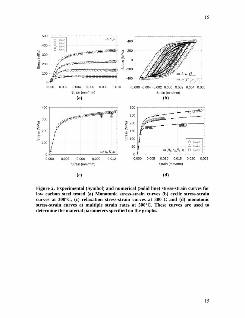
3. Model’s Material Parameters The material employed in this study is A572 Grade 50 Low Carbon Steel and its microstructure which is shown in Fig. 1, includes pearlite colonies and alpha-ferrite equiaxed grains. The average grain size is 53µm (ASTM 5). Volume fraction of the pearlite phase is 10 %. Figure 1. Optical micrograph of as-received A572 grade 50 steel etched for 5 seconds in 5 vol% nital. The microstructure is typical of normalized steel, consisting of pearlite colonies (dark phase) and alpha-ferrite (light phase) equiaxed grains. The pearlite colonies have a volume fraction of 10% and the grain size is 53 microns (ASTM 5). A series of strain-controlled tests were carried out on the as received steel, at both room and high temperature, to determine the various material parameters described above in order to fully identify the non-linear kinematic hardening model. The mechanical testing was carried out using a servo hydraulic test machine, equipped with a heat induction coil for the high temperature tests. The strain was measured with a quartz rod extensometer.

A monotonic test is carried out, to determine the modulus, E , and yield stress, k , of the material. Results of this rate at various loading conditions are shown in Fig. 2a. A series of strain-controlled fully reversed cyclic stress-strain tests (fatigue stress ratio = -1) are performed at strain ranges varying from ±0.2% to ±1% strain. A typical cyclic stress-strain curve at 300°C is shown in Fig. 2b. These loops are employed to generate the isotropic and kinematic hardening, as well as, viscosity and recovery parameters.

Figure 2. Experimental (Symbol) and numerical (Solid line) stress-strain curves for low carbon steel tested (a) Monotonic stress-strain curves (b) cyclic stress-strain curves at 300°C, (c) relaxation stress-strain curves at 300°C and (d) monotonic stress-strain curves at multiple strain rates at 500°C. These curves are used to determine the material parameters specified on the graphs.

The isotropic hardening parameter, b , is determined from the evolution of the peaks

of the cyclic stress-strain curves (Fig. 2b) maxQ and μ are calculated from the difference in the peak stress of the first cycle and the saturated cycle as a function of the maximum plastic strain achieved during loading [Maciejewski 2009, Nouailhas 1987, Nouailhas 1989, Zaki 2000]. The kinematic stress corresponds to the center of the linear part of the first reversible cyclic loop at each strain range (Fig. 2b). This stress is determined as a function of plastic strain to determine the materials parameters 1a , 1c , 2a and 2c .

To describe the time-dependent viscous stress term, a strain-controlled monotonic stress-relaxation test is performed, as seen in Fig. 2c. For this, during the periods of holding at a constant total strain, the stress and stress rate as a function of time is acquired. This is used to obtain the viscous stress in terms of plastic strain rate, from which, n and K , strain-rate sensitive parameters must be determined [Nouailhas 1989, Chaboche 1989, Lemaitre 1990]. The material constant, α , is taken to be the saturation limit of viscous stress for high plastic strain rates.

5

5

Time-dependent recovery parameters, 1β , 2β , are determined from the linear portion of the stress time curve. In this region it is assumed that R , k and viscous stress are constant and the time dependent stress is only coming from the time dependent back stress. These parameters, 1β , 2β , 1r and 2r , are optimized with stress-strain data at various strain rates. Strain rate sensitivity tests [Lemaitre 1990] are performed in which a specimen is loaded monotonically in strain-control at multiple strain rates, as shown in Fig. 2d.

The material parameter determination procedure, described above, has been applied to as received steel tested at temperatures ranging from 20-700°C, and is further detailed in references [Chaboche 1989, Lemaitre 1990, Maciejewski 2009, Nouailhas 1987, Nouailhas 1989, Zaki 2000]. The material constants from the above procedure are given in Table 1 for each temperature condition.

Table 1: Material parameters for as received A572 Grade 50 low carbon steel tested

at temperatures ranging from 20°C to 700°C.

Temperature/ Thermal History 20°C 300°C 500°C 600°C 700°C

E (GPa) 188 172 127 93 58 k (MPa) 100 71 27 11 3 a1 (MPa) 137 96 54 36 22

C1 1411 1411 1411 1411 1411 a2 (MPa) 1864 1753 1111 566 175

C2 1.15 1.15 1.15 1.15 1.15 b 78 78 78 78 78

Qmax (MPa) 86 78 31 1 -10 μ 1447 1447 1447 1447 1447 n 14 14 14 14 14

K (MPa) 155 349 304 227 107 α 5.5E+06 5.0E+06 1.0E+05 4.5E+00 9.9E-01

β1 (Pa2.58) 1.0E-21 9.9E-20 1.0E-15 1.0E-15 1.0E-15

β2 (Pa2.15) 4.6E-26 2.1E-16 1.0E-12 1.0E-12 1.0E-12 r1 2.58 2.58 2.58 2.58 2.58 r2 2.15 2.15 2.15 2.15 2.15

Several of the material constants, as described above, are temperature-dependent.

The material constants have been determined for five different temperatures, ranging from room temperature to 700°C. A linear interpolation to the material constants is generally used to extend a constitutive model working for any temperature, which may be

6

6

less accurate. A nonlinear form better describes the temperature span, and the formula used to fit the temperature-dependent material constants is given below:

00

tanhm

TC A CT⎛ ⎞⎛ ⎞= ∗ − +⎜ ⎟⎜ ⎟⎝ ⎠⎝ ⎠

(11)

Where C and T represent a material constant and temperature respectively, A , m , 0T ,

0C are unknown parameters which are figured out by curve fitting to C T− data. Fig. 3 shows two examples of the curve-fitting to the temperature-dependent

Young’s modulus and strain-rate sensitivity coefficient using the equation (11).

Figure 3. Modeling of temperature-dependent material constants (a) Young’s modulus, (b) isotropic hardening coefficient, Qmax.

The saturation of material constants at lower temperature was captured by the hyperbolic tangent function of temperature. The saturation values are defined by the parameters, A and 0C . The sensitivity of the material constant change with temperature is defined by the exponent, m . The reference temperature, 0T , defines the temperature at the middle of the transitional segment of the curve. The parameters for temperature-dependent material constants are listed in Table 2.

Table 2. Parameters in the formula for temperature-dependent material constants

Constant A 0T 0C m

E 187850.1 742.0 187743.8 2.8

k 100.6 520.8 99.6 2.3

1a 137.4 621.3 137.5 1.6

2a 1830.5 619.1 1864.3 3.9

maxQ 97.7 558.0 86.1 4.1

K 351.7 720.1 351.5 5.4

α 5.5E+06 437.3 5.5E+06 6.4

1β -1.0E-15 443.0 2.7E-27 18.8

2β -1.0E-12 443.0 3.2E-24 18.8

The temperature dependent and independent material constants are used to fully define the viscoplastic constitutive model. This model is then implemented in finite element

7

7

software to describe the material behavior under varying loading and temperature conditions. 4. Validation of UMAT code

The viscoplastic constitutive equations have been implemented into ABAQUS through a subroutine UMAT. A finite element model of uniaxial fatigue specimen was built to simulate the experimental tensile and fatigue tests. A comparison of experimental and numerical stress-strain curves is used to examine the implementation of the simulation model. A quarter 3D finite element model is shown in Fig. 4. The diameter of the cylindrical specimen is 6.35 mm and the gauge length is 10 mm. The block element with 8 nodes was used to mesh the geometry model. Nodes on the bottom plane were fixed in vertical direction, and symmetry boundary conditions were applied to the nodes on two side planes. To simulate the tensile tests, Nodes on the top plane were subjected to a displacement ramping from 0 to 0.1 mm within 2000 seconds. 4 simulation cases were done by assigning 4 different uniform temperatures to the whole model. The predicted stress-strain curves are shown in Fig. 5 and compared with the experimental results which show good agreement.

Figure 4. FE model of tensile tests Figure 5. Numerical and experimental stress-strain curves

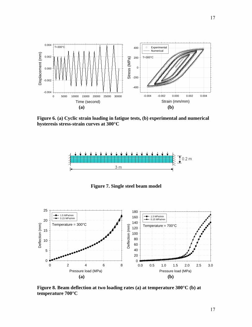
The quarter cylinder model was also used for the simulation of a fatigue test at

300°C. A cyclic displacement loading (see Fig. 6a) was applied to the nodes on the top plane.

Figure 6. (a) Cyclic strain loading in fatigue tests, (b) experimental and numerical hysteresis stress-strain curves at 300°C

The magnitude of applied displacement equals the value that the gauge length of the model times the strain that the element was subjected to. The displacement loading shows three strain ranges, ± 0.2%, ± 0.3% and ± 0.4%. 4 cycles were run under strain range ± 0.2%, 6 cycles under strain range ± 0.3%, and 3 cycles under strain range ± 0.4%. The cyclic test of three strain ranges used the same loading strain rate of 5x10-6 mm/mm/sec. The period of one cycle under strain range ± 0.2% is 1600 seconds, 2400 seconds under strain range ± 0.3%, and 3200 seconds under strain range ± 0.4%. The element stresses in vertical direction were output and plotted with the strains in the same direction. Both experimental and numerical hysteresis stress-strain curves are shown in Fig. 6b. The good agreement of experimental and numerical stress-strain curves validates the implementation of the UMAT code.

8

8

5. Finite element analysis and results

5.1 Simulation of single steel beam Numerical simulations were conducted using two finite element models, a simple

model of single steel beam and a complex model of steel-framed structure. Simulation of single steel beam

Single steel beam model (Fig. 7) was built to examine effects of loading rate and temperature on the beam deflection.

Figure 7. Single steel beam model

The two-dimensional beam is 3m long and 0.2m high. The element type of plain strain was assigned to all elements. Each element has a size of 0.1m long, 0.02m high. Uniform temperature field was applied to the beam and two temperature cases, 300°C and 700°C, were studied. Uniform pressure ramping up with time was also applied on the beam. Two cases of pressure ramping rate were investigated; 1.5 MPa/min and 0.15 MPa/min.

The beam deflections from the 4 simulation cases described above are compared in Fig. 8. which shows the evolution of the maximum beam deflections along with the ramping pressure.

Figure 8. Beam deflection at two loading rates (a) at temperature 300°C (b) at temperature 700°C

Fig. 8a compares the beam deflections generated at 300°C for two different pressure ramping rates while Fig. 8b shows the comparison at 700°C. At the temperature 300°C, the beam deflection is not dependent on the loading rate, however it shows dependency at the temperature 700°C. This result indicates that the 300°C is below the transition temperature of the material strain-rate sensitivity. If we compare the beam deflections under the same pressure load but at the two different temperatures, it becomes obvious that the beam deflection is larger at 700°C. The higher temperature reduces the strength of the material steel or the stiffness of the steel beam.

5.2 Simulation of steel-framed structure under fire condition Finite element analysis of steel-framed structures under fire condition uses a

sequentially coupled thermal-stress analysis [ABAQUS inc. 2006]. In this analysis, a transient heat transfer analysis is first performed to obtain temperature distribution history, and then a stress/deformation analysis is conducted to obtain structural deformation. Nodal temperatures are calculated in the transient heat transfer analysis and stored as a function of time in the heat transfer result file. The stress analysis uses the same geometry model with the same meshing as the heat transfer analysis. The temperature fields for the stress analysis are coupled with temperature results from transient heat transfer analysis.

A three-dimensional model of a multi-story structure was built, the dimensions of which are shown in Fig. 9.

9

9

Figure 9. Modeling of 3D steel-framed structure under fire condition

The structure has 2 cells with 8 box-shape columns and 8 I-shape beams. Each column is 12 meters high and each beam is 15 meters long. The dimensions of the column and beam cross-sections are shown in Fig. 9. We consider the beams and columns to be integral. 8-node block elements were used to mesh the structure as shown in Fig. 10.

Figure 10. Meshing of FE model of 3D steel-framed structure The element size is 0.5 meter in longitude direction of beam and column, and less than 0.04 meter in their transverse direction. The total number of elements is 19136.

5.2.1 Heat transfer analysis The finite element model was first employed to conduct transient heat analysis. The

material properties required for heat transfer analysis are shown in Table 3.

Table 3. Material properties for heat transfer analysis

Mass Density Thermal Conductivity Specific Heat 7800 kg/m3 50 J/m2°C 470 W/kg°C

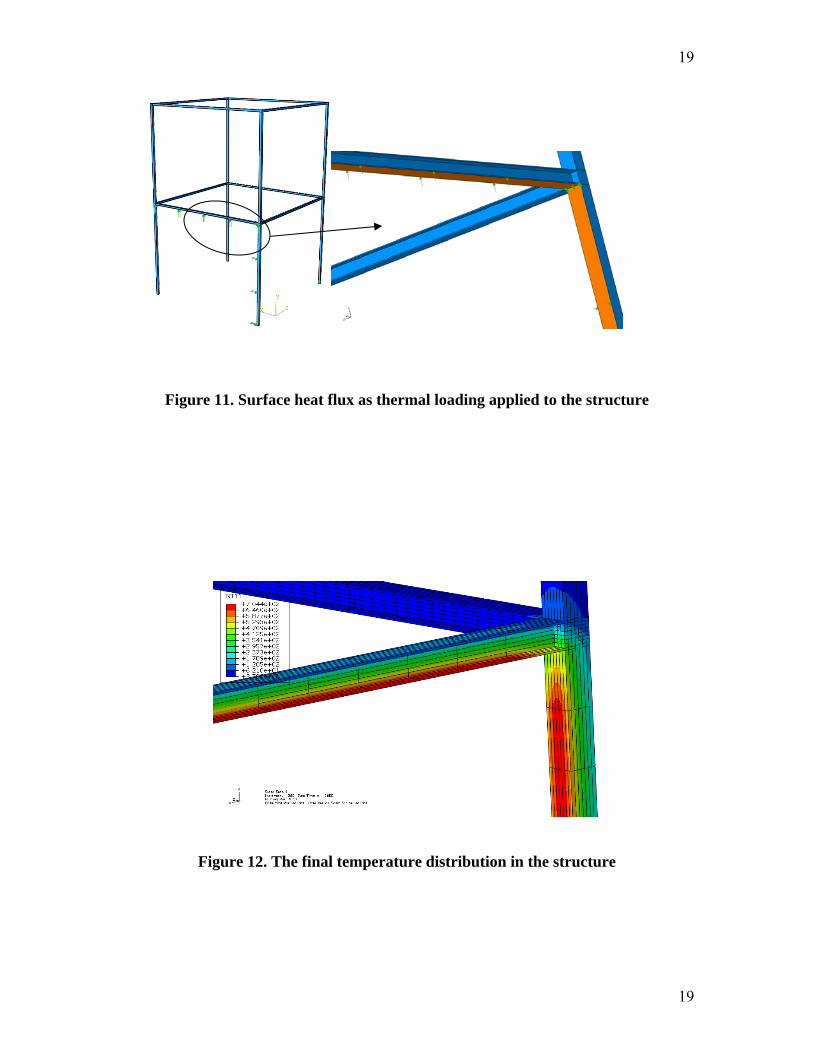
The element type was set as DC3D8 for heat transfer analysis. The room temperature 25°C was assigned to the steel-frame structure as the initial condition. A surface heat flux of 16 kW/m2 was applied on the bottom plane of one beam in the first floor, and 24 kW/m2 on the side plane of its connected column in order to simulate the appearance of a fire in the cell (see Fig. 11).

Figure 11. Surface heat flux as thermal loading applied to the structure The heat transfer duration is 1 hour. The calculated temperatures at all nodes and at different time are stored in the output file of heat transfer analysis. The output frequency of nodal temperatures is 0.2 Hz.

Fig. 12 shows the temperature distribution after 1 hour of heat transfer. The non-uniform temperatures across the sections of steel frames were observed.

Figure 12. The final temperature distribution in the structure

The higher temperature occurred to the positions near the surface where external heat flux was applied. Within 1 hour, the heat spread was confined in the mid cell of the first floor. Positions far away from the surface where the heat flux came in almost maintained their initial temperature of 25°C. Figs. 13-14 show the temperature history at 7 points on the heated beam’s and column’s cross-sections, respectively.

10

10

Figure 13. Temperature history of seven points on the beam’s cross-section

Figure 14. Temperature history of seven points on the column’s cross-section

The temperature at the monitored positions increases with time since the continuous heat flow increase the thermal energy of the structure. For the beam, the temperatures at points B1 and B2 are higher than those at points B3, B4 and B5, and much higher than those at points B6 and B7. For the column, the temperatures at points C1 and C2 are higher than those at points C3, C4 and C5, and much higher than those at C6 and C7. Although B1 and B2 are on the same heat flux surface, their temperatures are different. The temperature at B1 is higher than that at B2 because the position B2 is nearer to the web, which is the heat transfer path.

5.2.2 Stress/deformation analysis In the stress/deformation analysis, the element type was changed from heat transfer

type to stress analysis type C3D8, while the geometry remained the same. The developed UMAT was used as the material model. The four columns were fixed at their roots. A uniform pressure was applied on all beams and temperature field was assigned to the whole structure. The simulation consists of three loading steps. The first step is to increase the uniform pressure from zero to 0.04 MPa in 10 seconds, while keeping the temperature constant at 25°C. In the second step, the maximum pressure loading is maintained and the temperature field is coupled with the results obtained from the transient heat transfer analysis, and hence the duration of step 2 is 60 minutes. In the third step, both the pressure and temperature distribution in the structure is held constant for 30 minutes. Therefore, static stress/deformation analysis was performed with a time period of 90 minutes plus 10 seconds. The maximum time increment is 0.5 second. The control setting for the nonlinear effect of large displacement was activated in the simulation. The displacement, strain and stress results along with time were output from the stress analysis.

The final deformation of the three-dimensional two-story structure from the stress analysis using the viscoplastic constitutive model, discussed above, was examined. Among the four beams of the first floor, the beam subjected to the heat flux deflected more than other beams as expected. Fig. 15 shows the deflection history of two beams at the first floor (see Fig. 10).

Figure 15. The deflection history at the midspan of the heated and non-heated beams

The heated beam refers to the beam which had the heat flux applied to it, and the non-heated beam is a beam neighboring the heated beam. In the ten seconds of load step 1, the deflections of the two beams increase quickly due to the increasing pressure load. In this step, the two beams achieved the same amount of deflection due to geometrical symmetry, the same loading condition, and uniform structural temperature. In load step 2,

11

11

the deflection of the heated beam does not increase at the beginning although its temperatures increase. It is concluded that the beam’s deflection starts to increase when the applied load/stress becomes larger than the strength of the beam. The applied load did not change but the beam’s strength degraded with the increase of temperature. When the strength of the heated beam degraded below its stress level, the inelastic strain occurred as shown in Fig. 16, and the beam’s deflection started to increase slowly initially and then faster with the continuously increasing of the beam’s temperature.

Figure 16. Strain and stress history at the midspan of the heated beam In load step 3, the applied loading and the temperature distribution did not change (actually the applied stress relaxed as shown in Fig. 16), but the heated beam’s deflection continued to increase. The deflection increase in load step 3 was attributed to the creep deformation (that is, material strain-rate sensitivity) at elevated temperatures, which can be shown in Fig. 16.

6. Conclusions

The work in this paper describes a viscoplastic constitutive model that has been employed to simulate the flow behavior of structural steel A572 grade 50 steel at elevated temperatures. The material constants of a the model have been fitted as a function of temperature, thus allowing the implementation of the corresponding constitutive equations in a UMAT subroutine of the ABAQUS platform The validation of the UMAT has been carried out by comparing the experimental data with those obtained from the numerical simulations under the same applied load conditions. The finite element analysis of a three-dimensional steel-framed structure under fire condition has been performed using a simulation strategy of sequentially coupled thermal-stress analysis. The general conclusions of this study can be listed as follows: 1. The nonlinear material behavior of the low carbon structural steel at elevated

temperatures can be captured by unified constitutive equations, which consist of a nonlinear kinematic hardening model and a hyperbolic function for the modeling of temperature-dependent material constants.

2. The steel shows a transition temperature for the time-dependent plastic deformation. The strain-rate sensitivity transition is indicated by the trend of temperature-dependent material constants.

3. The heat transfer analysis of the 3D steel-frame structure shows the temperature distributed nonlinearly across the sections of the steel frame and along the length of beams and columns.

4. As the temperature increases, large bending or buckling deformation could occur to the steel-frame structure as a result of the degradation of the material’s strength below the applied stress level.

5. The time-dependent material behavior contributes to the structure’s bending or bucking when the applied temperature is higher than the strain-rate sensitivity transition temperature.

12

12

Acknowledgments This work has been supported by FM Global and the Department of Homeland Security Center of Excellence: Explosives Detection, Mitigation, and Response at the University of Rhode Island References ABAQUS Inc. (2006). ABAQUS Standard User’s Manual, 6.6 Edition. Chaboche, J.L., and Rousselier, G. (1983), On the Plastic and Viscoplastic Constitutive

Equations—Part I: Ruled Developed with Integral Variable Concept, Transactions of the ASME, Journal of Pressure Vessel Technology, 105, pp.123-133.

Chaboche, J.L., and Rousselier, G. (1983), On the Plastic and Viscoplastic Constitutive Equations—Part II: Application of Integral Variable Concepts to the 316 Stainless Steel, Transactions of the ASME, Journal of Pressure Vessel Technology, 105, pp. 159-164.

Chaboche, J.L. (1989), Constitutive Equations for Cyclic Plasticity and Cyclic Viscoplasticity, International Journal of Plasticity, 5, pp.247-302.

Kumar P, Nukala VV, White DW., A Mixed Finite Element for Three-Dimensional Nonlinear Analysis of Steel Frames, Comput Methods Appl Mech Engrg, 193, 2004, pp. 2507-2545.

Lemaitre, J., and Chaboche (1990), J.L., Mechanics of Solid Materials, Cambridge University Press, Cambridge, United Kingdom.

Li G.Q., Jiang S.C. (1999), Prediction to Nonlinear Behavior of Steel Frames Subjected to Fire, Fire Safety Journal, 32, pp.347-68.

Liew J.Y., Tang L.K., Holmaas T, Choo Y.S. (1998), Advanced Analysis for the Assessment of Steel Frames in Fire, Journal of Constructional Steel Research, 47, pp.19-45.

K. Maciejewski, Y. Sun, O. Gregory and H. Ghonem (2008), Deformation and Hardening Characteristics of Low Carbon Steel at Elevated Temperature, Material Science and Technology Conference and Exhibition, October 2008, Pittsburgh, Pennsylvania. Makelainen P, Outinen J, Kesti J. (1998), Fire design model for structural steel S420M

based upon transient-state tensile test results, Journal of Constructional Steel Research, 48, pp. 47-57.

Najjar, S.R., and Burgess, I.W. (1996), A Nonlinear Analysis for Three-Dimensional Steel Frames in Fire Conditions, Engineering Structures, 18(1), pp. 77-89.

Nouailhas, D. (1987), A Viscoplastic Modelling Applied to Stainless Steel Behavior, Proceedings of the Second International Conference on Constitutive Laws for Engineering Materials: Theory and Application, January 5-8, Tuscon, Arizona, U.S.A., pp.717-724.

Nouailhas, D.(1989), Unified Modeling of Cyclic Viscoplasticity: Application to Austenitic Stainless Steels, International Journal of Plasticity, 5, pp. 501-520.

Wang, Y.C., Lennon, T., and Moore, D.B. (1995), The Behavior of Steel Frames Subject to Fire, Journal of Constructional Steel Research, 35, pp. 291-322.

13

13

Zaki, A.S., and Ghonem, H. (2000), Modeling the Ratcheting Phenomenon in an Austenitic Steel at Room Temperature, Proceeding of the ASME 2000 Design, Reliability, Stress Analysis and Failure Prevention Conference, Baltimore, Maryland, U.S.A.,

14

14

100 µm100 µm100 µm

Figure 1. Optical micrograph of as-received A572 grade 50 steel etched for 5 seconds in 5 vol% nital. The microstructure is typical of normalized steel, consisting of pearlite colonies (dark phase) and alpha-ferrite (light phase) equiaxed grains. The pearlite colonies have a volume fraction of 10% and the grain size is 53 microns (ASTM 5).

15

15

Strain (mm/mm)0.000 0.002 0.004 0.006 0.008 0.010

Stre

ss (M

Pa)

0

100

200

300

400

500300°C500°C600°C700°C

,E k⇒

Strain (mm/mm)-0.006 -0.004 -0.002 0.000 0.002 0.004 0.006

Stre

ss (M

Pa)

-400

-200

0

200

400

max

1 1 2 2

, ,, , ,

b Qa C a Cμ⇒

⇒

(a) (b)

Strain (mm/mm)0.000 0.003 0.006 0.009 0.012

Stre

ss (M

Pa)

0

100

200

300

400

, ,n K α⇒

Strain (mm/mm)0.000 0.005 0.010 0.015 0.020 0.025

Stre

ss (M

Pa)

0

50

100

150

200

250

300

5e-4 s-1

5e-6 s-1

5e-7 s-11 1 2 2, , ,r rβ β⇒

(c) (d)

Figure 2. Experimental (Symbol) and numerical (Solid line) stress-strain curves for low carbon steel tested (a) Monotonic stress-strain curves (b) cyclic stress-strain curves at 300°C, (c) relaxation stress-strain curves at 300°C and (d) monotonic stress-strain curves at multiple strain rates at 500°C. These curves are used to determine the material parameters specified on the graphs.

16

16

Temperature (°C)0 100 200 300 400 500 600 700

E (M

Pa)

0

5e+4

1e+5

2e+5

2e+5

ExperimentalCurve Fit

Temperature (°C)0 100 200 300 400 500 600 700

Qm

ax (M

Pa)

-20

0

20

40

60

80

100

ExperimentalCurve Fit

(a) (b)

Figure 3. Modeling of temperature-dependent material constants (a) Young’s modulus, (b) isotropic hardening coefficient, Qmax.

Strain (mm/mm) 0.000 0.002 0.004 0.006 0.008 0.010

Stre

ss (M

Pa)

0

100

200

300

400Experimental Numerical

T=300°C

T=500°C

T=600°C

T=700°C

Figure 4. FE model of tensile tests Figure 5. Numerical and experimental stress-strain curves

17

17

Time (second)0 5000 10000 15000 20000 25000 30000

Dis

plac

emen

t (m

m)

-0.004

-0.002

0.000

0.002

0.004T=300°C

Strain (mm/mm)-0.004 -0.002 0.000 0.002 0.004

Stre

ss (M

Pa)

-400

-200

0

200

400 ExperimentalNumerical

T=300°C

(a) (b)

Figure 6. (a) Cyclic strain loading in fatigue tests, (b) experimental and numerical hysteresis stress-strain curves at 300°C

Figure 7. Single steel beam model

Pressure load (MPa)0 2 4 6 8

Def

lect

ion

(mm

)

0

5

10

15

20

251.5 MPa/min0.15 MPa/min

Temperature = 300°C

Pressure load (MPa)0.0 0.5 1.0 1.5 2.0 2.5 3.0

Def

lect

ion

(mm

)

020406080

100120140160180

1.5 MPa/min0.15 MPa/min

Temperature = 700°C

(a) (b)

Figure 8. Beam deflection at two loading rates (a) at temperature 300°C (b) at temperature 700°C

18

18

Figure 9. Modeling of 3D steel-framed structure under fire condition

Figure 10. Meshing of FE model of 3D steel-framed structure

19

19

Figure 11. Surface heat flux as thermal loading applied to the structure

Figure 12. The final temperature distribution in the structure

20

20

Time (seconds)

0 1000 2000 3000

Tem

pera

ture

(oC

)

0

200

400

600B1B2B3 B4B5B6B7

Figure 13. Temperature history of seven points on the beam’s cross-section

Time (seconds)

0 1000 2000 3000

Tem

pera

ture

(oC

)

0

200

400

600C1 C2C3 C4C5 C6C7

Figure 14. Temperature history of seven points on the column’s cross-section

C1 C2

C3C4 C5

C6

C7

B1 B2

B3 B4

B6 B7 B5

21

21

Time (minutes)

0 20 40 60 80 100

Def

lect

ion

(mm

)

0

10

20

30

40

50

Midspan of heated beamMidspan of nonheated beam

Figure 15. The deflection history at the midspan of the heated

and non-heated beams

Time (minutes)

0 20 40 60 80 100

Stra

in (m

m/m

m)

0.0000

0.0001

0.0002

0.0003

0.0004

0.0005

Stre

ss (M

Pa)

0

10

20

30

40

50

60

Strain at heated beam midspanStress at heated beam midspan

Figure 16. Strain and stress history at the midspan of the heated beam