thermo-viscoelastic-viscoplastic-viscodamage- healing...
TRANSCRIPT

THERMO-VISCOELASTIC-VISCOPLASTIC-VISCODAMAGE-
HEALING MODELING OF BITUMINOUS MATERIALS: THEORY
AND COMPUTATION
A Dissertation
by
MASOUD DARABI KONARTAKHTEH
Submitted to the Office of Graduate Studies of
Texas A&M University in partial fulfillment of the requirements for the degree of
DOCTOR OF PHILOSOPHY
August 2011
Major Subject: Civil Engineering

Thermo-Viscoelastic-Viscoplastic-Viscodamage-Healing Modeling of Bituminous
Materials: Theory and Computation
Copyright 2011 Masoud Darabi Konartakhteh

THERMO-VISCOELASTIC-VISCOPLASTIC-VISCODAMAGE-
HEALING MODELING OF BITUMINOUS MATERIALS: THEORY
AND COMPUTATION
A Dissertation
by
MASOUD DARABI KONARTAKHTEH
Submitted to the Office of Graduate Studies of Texas A&M University
in partial fulfillment of the requirements for the degree of
DOCTOR OF PHILOSOPHY
Approved by:
Co-Chairs of Committee, Rashid K. Abu Al-Rub Eyad A. Masad Committee Members, Dallas N. Little Anastasia Muliana Imad Al-Qadi Head of Department, John Niedzwecki
August 2011
Major Subject: Civil Engineering

iii
ABSTRACT
Thermo-Viscoelastic-Viscoplastic-Viscodamage-Healing Modeling of Bituminous
Materials: Theory and Computation. (August 2011)
Masoud Darabi Konartakhteh, B.S., Sharif University of Technology;
M.Sc., Sharif University of Technology
Co-Chairs of Advisory Committee: Dr. Rashid K. Abu Al-Rub Dr. Eyad A. Masad
Time- and rate-dependent materials such as polymers, bituminous materials, and soft
materials clearly display all four fundamental responses (i.e. viscoelasticity,
viscoplasticity, viscodamage, and healing) where contribution of each response strongly
depends on the temperature and loading conditions. This study proposes a new general
thermodynamic-based framework to specifically derive thermo-viscoelastic, thermo-
viscoplastic, thermo-viscodamage, and micro-damage healing constitutive models for
bituminous materials and asphalt mixes. The developed thermodynamic-based
framework is general and can be applied for constitutive modeling of different materials
such as bituminous materials, soft materials, polymers, and biomaterials. This
framework is build on the basis of assuming a form for the Helmohelotz free energy
function (i.e. knowing how the material stores energy) and a form for the rate of entropy
production (i.e. knowing how the material dissipates energy). However, the focus in this
work is placed on constitutive modeling of bituminous materials and asphalt mixes. A
viscoplastic softening model is proposed to model the distinct viscoplastic softening
response of asphalt mixes subjected to cyclic loading conditions. A systematic procedure
for identification of the constitutive model parameters based on optimized experimental
effor is proposed. It is shown that this procedure is simple and straightforward and yields
unique values for the model material parameters. Subsequently, the proposed model is
validated against an extensive experimental data including creep, creep-recovery,
repeated creep-recovery, dynamic modulus, constant strain rate, cyclic stress controlled,
and cyclic strain controlled tests in both tension and compression and over a wide range

iv
of temperatures, stress levels, strain rates, loading/unloading periods, loading
frequencies, and confinement levels. It is shown that the model is capable of predicting
time-, rate-, and temperature-dependent of asphalt mixes subjected to different loading
conditions.

v
DEDICATION
TO MY BELOVED PARENTS
Thank you for your endless patience, unconditional support, and continuous
encouragement.
TO MY LOVELY WIFE, AZADEH
Your love gave me the support needed in this journey.

vi
ACKNOWLEDGEMENTS
I am incredibly grateful to many people who helped me as I researched this topic. There
are far too many, to mention all of them; but I would like to thank several here.
First, I gratefully thank my advisor, Dr. Rashid K. Abu Al-Rub, whose guidance
and support has been beyond invaluable both for his technical expertise in this subject
and his overall nurturing of me as a researcher. Without him, this work would never
been accomplished.
I would also like to thank my advisory committee co-chair, Dr. Eyad Masad, who
provided me with his deep understanding on the subject. The innumerable fruitful
discussions that I had with him helped set me straight whenever I got lost in the subtle
twists of this difficult field. I also wish to thank my other advisory committee member,
Dr. Dallas Little, for his support and helpful discussions that we had on modeling the
healing phenomenon in bituminous materials and asphalt mixes. I would also like to
thank Drs. Anastasia Muliana and Imad Al-Qadi, my other advisory committee
members, for their patience in reading this dissertation and their many pertinent
comments. I also thank Dr. Robert Lytton for his insightful comments on the healing
response of asphalt mixes.
I also wish to thank all my fellow researchers who helped me in this research. I
truly value Dr. Chien-Wei Huang’s help and his significant contribution in this research.
His work served as a basis for mine presented here. Dr. Sun-Myung Kim, Maryam
Shakiba, and Taesun You were supportive and very insightful- I look forward to their
work on this topic! I also thank Mike Graham for the fruitful discussions we had during
the early stages of this work. Mahmood Ettehad and Ardeshir Tehrani have always been
available and open to discussions, and I thank them for that.
I would like to offer special thanks to Drs. Gordon Airey, Richard Kim, and
Emad Ghasem for providing us data from wide range mechanical tests on asphalt mixes
that strongly aided my understanding of the mechanical response of asphalt mixes.

vii
I gratefully acknowledge the Asphalt Research Consortium for funding my
research.

viii
NOMENCLATURE
Symbol Definition Symbol Definition
New symbols introduced in Chapter II
Total strain tensor Y Damage force
nve Nonlinear viscoelastic strain tensor
vd Damage viscosity parameter
vp Viscoplastic strain tensor 0 , ,Y q k ,
vdd Damage model parameters
e Deviatoric strain tensor vd Deviatoric component of the viscodamage force
kk Volumetric strain vd Viscodamage dynamic loading condition
p Effective viscoplastic strain
RW , R
Pseudo strain energy and pseudo strain
eff Total effective strain 0D , D Instantaneous and transient creep compliances
Stress tensor nD , n Prony series’ coefficients
S Deviatoric stress tensor 0g , 1g , 2g Viscoelastic nonlinear parameters
kk Volumetric stress Reduced time
1I First stress invariant Ta , sa , ea Temperature, strain or stress, and environmental shift factors
2J , 3J The second and the third deviatoric stress invariants ijq Hereditary integral
E , G , K Elastic, Shear, and bulk moduli
“tr” Designates trial values

ix
Symbol Definition Symbol Definition
J , B Shear and bulk compliances
vp Viscoplastic multiplier
Poisson’s ratio f , F Viscoplastic yield and potential functions
ij Kronecker delta Viscoplastic dynamic yield surface
“ ” Designate the effective (undamaged) configuration
vp Viscoplastic viscosity parameter
Damage density variables Overstress function
Continuity scalar 0, , ,N
1 2, , , vpd Viscoplastic model parameters
A , A
Cross-sectional area in the damaged and effective configuration
Macaulay brackets
DA Area of the micro-damages
0y Initial yield stress
c Critical damage density Isotropic hardening function
vp
Deviatoric component of the viscoplasticity yield surface
1 , 2 , 3 Temperature coupling term parameters
T Temperature 0T Reference temperature
R Residual strain ijklS Tangent compliance
New symbols introduced in Chapter III
Mass density u
Displacement vector
b Body force vector extr External heat
x
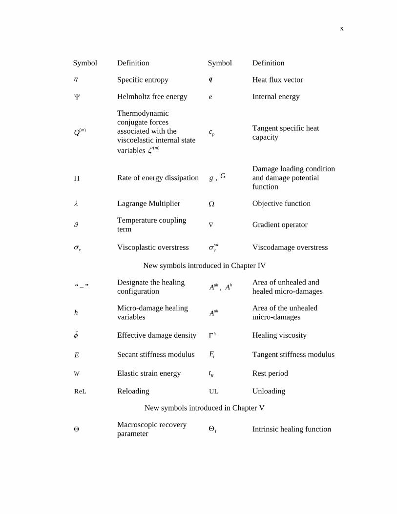
Symbol Definition Symbol Definition
Specific entropy q Heat flux vector
Helmholtz free energy e
Internal energy
( )mQ
Thermodynamic conjugate forces associated with the viscoelastic internal state variables ( )m
pc Tangent specific heat capacity
Rate of energy dissipation g , G Damage loading condition and damage potential function
Lagrange Multiplier Objective function
Temperature coupling term
Gradient operator
v Viscoplastic overstress vdv Viscodamage overstress
New symbols introduced in Chapter IV
“ ” Designate the healing configuration
uhA , hA Area of unhealed and healed micro-damages
h Micro-damage healing variables
uhA Area of the unhealed micro-damages
Effective damage density h Healing viscosity
E Secant stiffness modulus tE Tangent stiffness modulus
W Elastic strain energy Rt Rest period
ReL Reloading UL Unloading
New symbols introduced in Chapter V
Macroscopic recovery parameter I Intrinsic healing function

xi
Symbol Definition Symbol Definition
Wetting distribution function b Bond strength
cW Work of cohesion ba Rate of crack shortening
Healing process zone h , 1b , 2b Micro-damage healing model parameters
New symbols introduced in Chapter VI
H Healing force Kinematic hardening
intP Internal power extP External power
*
intP Internal virtual power *
extP External virtual power
“ene” Designates energetic component
“dis” Designates dissipative component
New symbols introduced in Chapter VII
*D Dynamic compliance D Storage compliance
D Loss compliance ,softvp Viscoplastic softening viscosity parameter
vpq Viscoplastic softening internal state variable 1S , 2S , 3S Viscoplastic softening
model parameters
,softvp Viscoplastic softening dynamic memory surface
New symbols introduced in Chapter VIII
“^” Designates nonlocal variables
Intrinsic material length scale
2 Laplacian operator mng Nonlocal coefficients

xii
Symbol Definition Symbol Definition
edtE
Elastic-damage tangent stiffness
algtE
Algorithmic elastic-damage tangent stiffness

xiii
TABLE OF CONTENTS
CHAPTER Page I INTRODUCTION AND LITERATURE REVIEW…………... 1
1.1. Problem Statement………………………………….. 1 1.2. Background and State of the Art……………………. 6 1.2.1. Viscoelasticity……………………………..... 6 1.2.2. Viscoplasticity……………………………..... 7 1.2.3. Viscodamage……………………………....... 9 1.2.4. Micro-Damage Healing..…………................. 11 1.3. Scope and Objective……………………………........ 14 1.4. Organization of the Dissertation……………………. 15
II A THERMO-VISCOELASTIC-VISCOPLASTIC-VISCODAMAGE MODEL FOR ASPHALTIC MATERIALS 17
2.1. Introduction…………………………………...…….. 17 2.2. Total Strain Additive Decomposition………………. 18 2.3. Effective (Undamaged) Stress Concept…………….. 18 2.4. Nonlinear Thermo-Viscoelastic Model……………... 22 2.5. Thermo-Viscoplastic Model……………………….... 24 2.6. Thermo-Viscodamage Model……………………….. 29 2.7. Numerical Implementation………………………….. 35 2.7.1. Implementation of the Viscoelastic Model…. 36 2.7.2. Implementation of the Viscoplastic Model…. 38 2.7.3. Implementation of the Viscodamage Model... 41 2.8. Application of the Model to Asphalt Concrete:
Model Calibration………………………………….. 43 2.8.1. Identification of the Viscoelastic Model
Parameters...………………………………… 44 2.8.2. Identification of the Viscoplastic Model
Parameters…………………………………... 46 2.8.3. Identification of the Viscodamage Model
Parameters...………………………………… 49 2.8.4. Identification of the Model Parameters
Distinguishing between Loading Modes...….. 51 2.8.5. Identification of the Temperature Coupling
Term Model Parameters…..………………… 52 2.9. Application of the Model to Asphalt Concrete:
Model Validation…………………………………... 57

xiv
CHAPTER Page
2.9.1. Model Validation against Creep-Recovery Tests………………………………………… 58
2.9.2. Model Validation against Creep Test...……... 61 2.9.3. Model Validation against Uniaxial Constant
Strain Rate Tests…………………………... 64 2.9.4. Model Validation against Repeated Creep-
Recovery Tests…..………………………….. 69 2.10. Conclusions…...…………………………………… 76
III THERMODYNAMIC CONSISTENCY OF THE THERMO-VISCOELASTIC-VISCOPLASTIC-VISCODAMAGE CONSTITUTIVE MODEL……………………………………. 79
3.1. Introduction…………………………………………. 79 3.2. Basic Thermodynamic Formulations……………….. 80 3.3. Specific Free Energy Function……………………… 86 3.4. Viscoelastic Constitutive Model……………………. 90 3.5. Viscoplastic Constitutive Model……………………. 94 3.6. Viscodamage Constitutive Model…………………... 98 3.7. The Heat Equation………………………………….. 100 3.8. Conclusions…………………………………………. 102
IV A CONTINUUM DAMAGE MECHANICS FRAMEWORK FOR MODELING MICRO-DAMAGE HEALING………….. 104
4.1. Introduction…………………………………………. 104 4.2. Micro-Damage Healing Configuration……………... 108 4.3. The Stiffness Moduli in Different Configurations….. 113 4.3.1. Strain Equivalence Hypothesis……………… 116 4.3.2. Elastic Strain Energy Equivalence
Hypothesis……..……………………………. 118 4.3.3. Power Equivalence Hypothesis…………….. 119 4.4. Damage and Healing Models and the Numerical
Implementation………………..…………………….. 122 4.4.1. Damage and Healing Evolution Functions….. 122 4.4.2. Numerical Implementation for Different
Transformation Hypotheses……..………….. 124 4.5. Numerical Results and Examples………………….... 128 4.5.1. Example 1: Different Transformation
Hypotheses…..……………………………… 128 4.5.2. Effect of Healing on Stiffness Recovery…..... 134

xv
CHAPTER Page 4.5.3. Effect of Healing and Damage Models on
Predicting the Fatigue Damage……………... 138 4.5.3.1. Rate-independent damage model………. 139 4.5.3.2. Rate-dependent damage model………… 140 4.5.3.3. Rate-dependent damage and healing
models……………………………….. 144 4.6. Conclusions…………………………………………. 146
V A MICRO-DAMAGE HEALING MODEL THAT IMPROVES PREDICTION OF FATIGUE LIFE IN ASPHALT MIXES……………………………………………. 148
5.1. Introduction.………………………………………… 148 5.2. Healing Natural Configuration…………………….... 149 5.3. Constitutive Model………………………………….. 151 5.3.1.Thermo-Viscoelastic-Viscoplastic-
Viscodamage Model…...…..………………… 151 5.3.2. Proposed Micro-Damage Healing Model…... 151 5.4. Finite Element Implementation…………………….. 156 5.5. Application of the Model for Prediction of Response
of Asphalt Mixes…………………………………… 158 5.5.1. Identification of the Micro-Damage Healing
Model Parameters..…………………………. 158 5.5.2. Prediction of Fatigue Life in Asphalt Mixes... 159 5.6. Effect of Healing Model Parameters………………... 171 5.7. Conclusions…………………………………………. 174
VI A NEW GENERAL THERMODYNAMIC-BASED FRAMEWORK FOR CONSTITUTIVE MODELING OF TIME- AND RATE-DEPENDENT MATERIALS…………… 177
6.1. Introduction………………………………………… 177 6.2. Natural Healing Configuration and Transformation
Hypothesis…………..………………………………. 182 6.3. Thermodynamic Framework………………………... 183 6.3.1. Internal and External Expenditures of Power. 183 6.3.2. Principle of Virtual Power………………….. 186 6.3.3. Non-Associative Plasticity/Viscoplasticity
Based on Principle of Virtual Power...……… 189 6.3.4. Internal State Variables and Clausius-Duhem
Inequality……...…………………………...... 196

xvi
CHAPTER Page
6.3.5. Maximum Rate of the Energy Dissipation Principle……………..……………………… 200
6.4. Application to Bituminous Materials..…………….... 203 6.4.1. Thermo-Viscoelastic Constitutive Equation... 204 6.4.2. Thermo-Viscoplastic Constitutive Equation... 208 6.4.3. Thermo-Viscodamage Constitutive Equation. 212 6.4.4. Thermo-Healing Constitutive Equation…….. 214 6.5. Heat Equation……………………………………….. 216 6.6. Conclusions…………………………………………. 219
VII VALIDATION OF THE THERMO-VISCOELASTIC-
VISCOPLASTIC-VISCODAMAGE-HEALING MODEL AGAINST THE ALF DATA…………………. ……………… 221
7.1. Introduction………………………………………… 221 7.2. Materials... …………………………………………. 222 7.3. Model Calibration in Compression………..……….. 222 7.3.1. Identification of the Thermo-Viscoelastic
Model Parameters...…………………..……... 223 7.3.2. Identification of the Viscoplastic Model
Parameters……………………………..……. 224 7.3.3. Viscoplastic Softening Model and the
Viscoplastic Softening Memory Surface…..... 228 7.4. Model Validation in Compression…...……………... 234 7.4.1. Model Validation against Constant Loading
Time Test (CLT)……...…………………….. 234 7.4.2. Model Validation against Variable Loading
Time Test (VT)..…………………………….. 239 7.4.3. Model Validation against Reversed Variable
Loading Time Test (RVT) …………...…….. 241 7.5. Effect of Viscoplastic Softening Model on the
Mechanical Response………………...……………... 242 7.6. Identification of the Model Parameters in Tension.… 246 7.6.1. Viscoelastic-Viscoplastic Parameters in
Tension and Time-Temperature Shift Factors 247 7.6.2. Viscodamage Model Parameters in Tension... 248 7.7. Validation of the Model against the Uniaxial
Constant Strain Rate Test in Tension……………….. 258 7.8. Validation of the Model against the Cyclic Stress
Controlled Tests in Tension……………………….... 266 7.9. Validation of the Model against the Cyclic Strain
Controlled Test in Tension….……………………… 271

xvii
CHAPTER Page 7.10. Conclusions……………………………………… 283
VIII NUMERICAL TECHNIQUES FOR FINITE ELEMENT
IMPLEMENTATION OF GRADIENT-DEPENDENT CONTINUUM DAMAGE MECHANICS THEORIES………. 285
8.1. Introduction…………………………………………. 285 8.2. Continuum Damage Model…………………………. 289 8.2.1. Local Continuum Damage Model…………... 289 8.2.2. Nonlocal Damage Model…………….……... 291 8.3. Computation of Nonlocal Damage Density.………... 293 8.4. Nonlocal Gradient-Dependent Tangent Moduli.……. 298 8.5. Numerical Examples…………………………..……. 301 8.5.1. Fixed Plate in Tension………………………. 302 8.5.2. Strip in Tension……. …………..…………... 310 8.6. Effect of Different Parameters on Damage
Localization……………………………………..….. 316 8.6.1. Effect of Parameters and …………..…. 316 8.6.2. Length Scale Effect... …..…………………... 319 8.7. Conclusions…………………………………………. 321
IX FINITE ELEMENT AND CONSTITUTIVE MODELING TECHNIQUES FOR PREDICTION OF RUTTING IN ASPHALT PAVEMENTS....…………………. ……………… 323
9.1. Introduction…………………………………………. 323 9.2. Material Constitutive Model..………………………. 327 9.3. Description of the Finite Element Simulations..……. 327 9.3.1. Geometry of the Finite Element Model…….. 328 9.3.2. Applied Wheel Loading Assumptions……… 330 9.3.2.1. Wheel loading assumptions in 2D
simulations………………………..…… 331 9.3.2.2. Wheel loading assumptions in 3D
simulations…………………………….. 332 9.4. Material Parameters……………………....………… 333 9.5. Rutting Predictions.……………………....………… 334 9.5.1. 2D Simulation Results……………… ……. 335 9.5.2. 3D Simulation Results……………… ……… 341 9.6. Extrapolation of the Rutting in 3D.……....………… 348 9.7. Comparison with Experimental Results.….………… 351 9.8. Conclusions………………………………………… 354

xviii
CHAPTER Page
X CONCLUSIONS AND RECOMMENDATIONS..…………… 356 10.1. Summary of Findings.………………....…………... 356 10.1.1. Thermo-Viscoelasticity..……………..……. 356 10.1.2. Thermo-Viscoplasticity..…………….…….. 356 10.1.3. Thermo-Viscodamage....…………….…….. 357 10.1.4. Micro-Damage Healing..…………….…….. 359 10.1.5. Viscoplastic Softening....…….……….……. 360 10.1.6. Thermodynamic Consistency of the
Proposed Model…….....…………….…….. 361 10.1.7. Model Validation...….....…….……….……. 362 10.1.8. Performance Simulations...………….…….. 363 10.2. Recommended Areas of Future Research…………. 364 REFERENCES…………………………………………………....…………… 368 VITA…………………………………………………………………………... 391

xix
LIST OF FIGURES
FIGURE Page 1.1 Rutting in the asphalt pavements as a result of evolution of the
viscoplastic strain…….…………………………………….……… 2 1.2 X-Ray images of the cross-section of an asphalt mixture
laboratory specimen subjected to triaxial loading.………………. 3 2.1 Schematic representation of the effective and nominal
configurations……………………………………………………… 20 2.2 Schematic illustration of the extended Drucker-Prager yield
surface [Eqs. (2.22) and (2.23)]. (a) In the deviatoric plane; (b) In the meridional plane……………………………………………… 27
2.3 Schematic illustration of the influence of the stress path on the
modified Drucker-Prager yield surface…………………………… 28 2.4 Schematic illustration of the viscodamage nucleation criterion…... 34 2.5 The flow chart of the recursive-iterative algorithm for
implementation of the viscoelastic model………………………… 38 2.6 The flow chart of the recursive-iterative Newoton-Raphson
algorithm for implementation of the coupled viscoelastic-viscoplastic model………..……………………………………… 42
2.7 A schematic creep-recovery test………………………………… 45 2.8 Identification of the viscoelastic and viscoplastic model
parameters using a creep-recovery test at the reference temperature (i.e. 20oT C ) when the applied stress is 1500kPa and the loading time is 30 sec. (a) Separation of the viscoelastic and viscoplastic strains using the experimental data; (b) Experimental and model predictions for the viscoelastic strain and the viscoplastic strain; (c) Experimental and model prediction of the total strain………. 48
2.9 Model predictions and experimental measuremenst for the creep
test at the reference temperature (i.e. 20oT C ) and two different stress levels... ……………………………………………………… 51

xx
FIGURE Page 2.10 Model predictions and experimental measuremenst for the creep
test in tension at 20oC and different stress levels………...……… 52 2.11 Experimental data for creep compliance at 10T , 20, and 40oC .
(a) Before applying the temperature time-shift factor. (b) After applying the temperature time-shift factor……………………… 54
2.12 Model predictions and experimental measuremenst for the creep
test at different temperatures in order to identify the temperature coupling term parameters for the viscodamage model…………… 55
2.13 The procedure for identification of the thermo-viscoelastic-
viscoplastic-viscodamage constitutive model parameters………… 57 2.14 Experimental measurements and model predictions for creep-
recovery test in compression at 10oT C ; (a) 2000 kPa, (b) 2500 kPa………………………………………………………. 59
2.15 Experimental measurements and model predictions for creep-
recovery test in compression at 20oT C ; (a) 1000 kPa, (b) 1500 kPa………………………………………………………... 60
2.16 Experimental measurements and model predictions for creep-
recovery test in compression at 40oT C ………………………… 61 2.17 Experimental measurements and model predictions for the creep
test in compression at different temperatures and stress levels….. 62 2.18 Experimental measurements and model predictions for creep test
in tension. (a) 10oT C ; (b) 20oT C ; (c) 35oT C ……………. 63 2.19 (a) Comparison of experimental measurements and model
predictions for the constant strain rate test in compression when 0.005 sec-1. (b) Damage density versus strain for model
predictions presented in (a) ……………………………………… 65 2.20 (a) Comparison of experimental measurements and model
predictions for the constant strain rate test in compression when 0.0005 sec-1. (b) Damage density versus strain for model
predictions presented in (a)…… ………………………………… 66

xxi
FIGURE Page 2.21 (a) Comparison of experimental measurements and model
predictions for the constant strain rate test in compression when 0.00005 Sec-1. (b) Damage density versus strain for model
predictions presented in (a)…….………………………………… 67 2.22 (a) Experimental measurements and model predictions for the
constant strain test in tension when 20oT C . (b) Damage density versus strain for model predictions presented in (a)……………… 68
2.23 (a) Comparison between model results and experiments for
repeated creep-recovery test in compression when LT= 120 sec and UT=100 sec. (b) Damage density versus time………………… 70
2.24 Comparison between model results and experiments for repeated
creep-recovery test in compression. (a) LT= 60sec and UT=100sec; (b) LT= 60sec and UT=1500sec…………………… 72
2.25 (a) Comparison between model results and experiments for
repeated creep-recovery test in tension when LT= 120 sec and UT=100 sec. (b) Damage density versus time…………………… 74
2.26 Comparison between model results and experiments for repeated
creep-recovery test in tension. (a) LT= 60sec and UT=50sec; (b) LT= 60sec and UT=100sec; (c) LT=60sec and UT=1500sec…… 75
4.1 Schematic representation of the stress-strain response for a loading
(path “AB”), unloading (Path “BC”), and reloading (path “CD”) cycle. The stress-strain response during the unloading is nonlinear and also the tangent stiffness at the end of the unloading (i.e. UL
,t CE )
is less than the tangent stiffness modulus at the beginning of the reloading (i.e. ReL
,t CE )………………………………………………. 105 4.2 Schematic representation of: (a) the damaged partially healed
cylinder in tension; (b) the nominal configuration; (c) the healing configuration; and (d) the effective configuration. The nominal configuration includes the intact material, unhealed damages, and healed micro-damages; the healing configuration includes the intact material and the healed micro-damages and the effective configuration only includes the intact material…………………. 109

xxii
FIGURE Page 4.3 Schematic illustration of three possible paths for point “A” on the
stress-strain curve………………………...………………………. 114 4.4 A flowchart showing the general finite element implementation
procedure of the elastic-damage-healing model using different transformation hypotheses……………………………………….. 127
4.5 Model predictions for a uniaxial constant strain rate test using
different transformation hypothesis…………………….………… 129 4.6 Model predictions for a uniaxial constant stress rate test using
different transformation hypothesis…………………….………… 132 4.7 Model predictions of the secant stiffness moduli for both uniaxial
constant stress and uniaxial constant strain rate tests using different transformation hypotheses……………………………… 133
4.8 Loading history for the example simulated in Section 4.5.2...…… 135 4.9 (a) Stress-time; (b) stress-strain diagrams for the loading history
shown in Figure 4.7. Model predictions show more recovery in the stiffness during the reloading as Rt and consequently the healing
variable increases……...……...……...……...……...……...……... 136 4.10 (a) Effective damage density versus the normalized rest time;
smaller values for the effective damage density at the end of the rest time as the rest time increases; and (b) healing variable versus the normalized rest time; more damages heal as the rest time increases…………………………...……...……...……...……...… 137
4.11 The loading history for the examples presented in Section 4.5.3… 139 4.12 Model response when using the rate-independent damage model.. 140 4.13 Model responses for the rate-dependent damage model when
healing is not considered. (a) Stress-strain response; model predicts nonlinear response during the unloading and loading, hysteresis loops form and energy dissipates at each cycle; (b) Effective damage density versus time; damage density evolves during both loading and unloading at each cycle; however, the rate of damage evolution decreases as the number of loading cycles increases…………………………………………………………… 141

xxiii
FIGURE Page 4.14 Illustration of the anisotropic damage which has been postulated
by Ortiz (1985) to model the nonlinear stress-strain response during the unloading. (a) A schematic RVE with two embedded cracks “A” and “B”; (b) during the loading crack “B” opens and contributes to the degradation of the stiffness; and (c) during the unloading crack “A” opens while partial crack closure occurs at crack “B”. However, the net effect causes the stiffness modulus to degrade during the unloading……………………………………. 142
4.15 Model response for the rate-dependent damage and healing
models. (a) Stress-strain response; the hysteresis loops tend to converge to a single one as the number of loading cycles increases and model predictions also show the jump in the tangent stiffness modulus at unloading-loading point. (b) Effective damage density versus time; the effective damage density decreases during the unloading as a result of healing and reaches a plateau at large number of loading cycles. (c) Healing variable versus time; healing variable increases at small strain levels (close to unloading-loading points), and healing variable decreases during the loading since the total damaged area increases……………… 145
5.1 Extension of the effective stress concept in continuum damage
mechanics to damaged-healed materials.......................................... 149 5.2 Flowchart for numerical implementation of the proposed coupled
thermo-viscoelastic-viscoplastic-viscodamage-healing constitutive model……………………………………………………………… 157
5.3 The procedure for identification of the coupled thermo-
viscoelastic-viscoplastic-viscodamage-healing constitutive model parameters…….…………………………………………………… 159
5.4 Repeated creep-recovery test in compression with 120sec loading
time and 100sec resting period…………………………………… 161 5.5 Repeated creep-recovery test in compression with 60sec loading
time and 100sec resting period………………………………..… 162 5.6 Repeated creep-recovery test in compression with 60sec loading
time and 1500sec resting period………….……………………… 165

xxiv
FIGURE Page 5.7 Repeated creep-recovery test in tension with 120sec loading time
and 100sec resting period…………...…………………………… 166 5.8 Repeated creep-recovery test in tension with 60sec loading time
and 50sec resting period………….……………………………… 168 5.9 Repeated creep-recovery test in tension with 60sec loading time
and 100sec resting period…………...…………………………… 169 5.10 Repeated creep-recovery test in tension with 60sec loading time
and 1500sec resting period………………………………………… 170 5.11 Effect of healing viscosity parameter 0
h on fatigue behavior of asphalt mixes. (a) total strain versus time and (b) effective damage density versus time………………………………………………. 172
5.12 Effect of damage history parameter 1b on fatigue behavior of
asphalt mixes when 30 1.0 10 / sech and 2 0b …..…………… 173
5.13 Effect of healing history parameter 2b on fatigue behavior of
asphalt mixes when 30 1.0 10 / sech and 1 0b …...…………… 175
7.1 Complex modulus data in compression at different temperatures
before and after the time-temperature shift……………………… 225 7.2 Stress history for the Variable Loading (VL) test………………… 226 7.3 Model predictions and experimental measurements for the VL test
at 55oC…………………………………………………………….. 227 7.4 Schematic representation of the concept of the viscoplastic
softening memory surface………………………………………… 231 7.5 Experimental measurements and model prediction with and
without viscoplastic memory surface for the variable loading test (VL) at 55oC in compression.……………………………………... 233
7.6 Schematic representation of the stress input for the constant
loading time test (CLT). NCSU database includes CLT tests for four different loading times (LT) of 0.1, 0.4, 1.6, and 6.4 sec…… 234

xxv
FIGURE Page 7.7 Experimental measurements and model prediction with and
without viscoplastic memory surface for the constant loading and time test (CLT) at 55oC in compression when the loading time is 0.1sec……………………………………………………………… 236
7.8 Experimental measurements and model prediction with and
without viscoplastic memory surface for the constant loading and time test (CLT) at 55oC in compression when the loading time is 0.4 sec……………………………………………………………… 237
7.9 Experimental measurements and model prediction with and
without viscoplastic memory surface for the constant loading and time test (CLT) at 55oC in compression. (a) loading time is 1.6sec; (b) loading time is 6.4sec…………………………………………. 238
7.10 Schematic representation of stress input in variable loading time
test (VT). The unloading time (UT) is constant and equals to 200 sec………................................................................................ 239
7.11 Experimental measurements and model prediction with and
without viscoplastic memory surface for the variable loading time test (VT) at 55oC in compression. (a) rest period is 0.05sec; (b) rest period is 1sec; (c) rest period is 200sec……………………… 240
7.12 Schematic representation of stress input in the reversed various
loading time test (RVT).…………………………………………. 241 7.13 Experimental measurements and model prediction with and
without viscoplastic memory surface for the reversed variable loading time test (RVT) at 55oC in compression………………… 242
7.14 Effect of the viscoplastic softening viscosity parameter ,softvp on
the evolution of the viscoplastic softening internal state variable vpq . The other parameters are selected as : 1 0.3S and 2 0S …… 243
7.15 Effect of the viscoplastic softening parameter 1S on the evolution
of the viscoplastic softening internal state variable vpq . The other
parameters are selected as : ,soft 0.001 / secvp and 2 0S ………… 244

xxvi
FIGURE Page 7.16 Effect of viscoplastic softening model parameters on the softening
response of materials. (a) Effect of 2S parameter when ,soft 0.001 / secvp , 1 0.3S , and 3 0S ; (b) Effect of 3S parameter
when ,soft 0.001 / secvp , 1 0.3S , and 52 2 10 kPaS …………… 245
7.17 The complex compliance data at different temperatures. (a) before
time-temperature shift factor; (b) after time-temperature shift…. 248 7.18 Predicted viscoplastic strain versus the total applied strain at 5oC
when the strain rate is 1 10-4/sec.………………………………… 249 7.19 Stress-strain curves at 5oC which have been used in identifying the
viscodamage model parameters…………………………………… 251 7.20 The identified damage density versus time and strain for different
constant strain rate tests at 5oC…………………………………… 252 7.21 Rate of the damage density versus strain for the constant strain
rate tests at 5oC…………………………………………………… 253 7.22 Plot of the damage rate versus the normalized effective damage
density for identification of the parameters q and vd ………….. 254 7.23 Rate of the damage density versus the effective damage force Y
for constant strain rate tests at 5oC……………………………… 255 7.24 Plot of the damage rate versus the strain for identification of the
parameters k and vd . …………………………………………… 256 7.25 Plot of the natural logarithm of the damage rate versus strain for
different strain rates at 5oC showing that the damage rate does not correlate with an exponential function of strain…………………… 257
7.26 Model predictions and experimental measurements for the
constant strain rate test in tension at 5oC when strain rates are: (a) 7 10-6/sec; (b) 2.1 10-5/sec; (c) 3 10-5/sec; (d) 5.5 10-5/sec… 258
7.27 Model predictions and experimental measurements for the
constant strain rate test in tension at 12oC when strain rates are: (a) 2.7 10-4/sec; (b) 4.6 10-4/sec……………………………………. 260

xxvii
FIGURE Page 7.28 Predicted damage density versus strain for the constant strain rate
test at 12oC. ……………………………………………………… 261 7.29 Model predictions and experimental measurements for the
constant strain rate test in tension at 25oC when strain rates are: (a) 5 10-4/sec; (b) 1.5 10-3/sec; (c) 4.5 10-3/sec; (d) 1.35 10-2
/sec………………………………………………………………... 261 7.30 Predicted damage density versus strain for the constant strain rate
test at 25oC. ……………………………………………………… 263 7.31 Model predictions and experimental measurements for the
constant strain rate test in tension at 40oC when strain rates are: (a) 3 10-4/sec; (b) 10-3/sec; (c) 3 10-3/sec…………………………... 263
7.32 Predicted damage density versus strain for the constant strain rate
test at 40oC. ……………………………………………………… 265 7.33 Comparison of the viscodamage time-temperature shift factor and
the viscoelastic-viscoplastic time-temperature shift factor (identified from dynamic modulus test) when the reference temperature is 10oC……………………………………………… 266
7.34 Schematic representation of loading history for Controlled Stress
cyclic test in tension. ……………………………………………… 267 7.35 Compasrison of the model prediction using viscoelastic-
viscoplastic model and experimental data for the cyclic stress control test at 19oC when the stress amplitude is 750kPa. (a) Loading cycles 1-30; (b) Loading cycles 970-980……………….. 268
7.36 Comparison of the VE-VP-VD model prediction and experimental
data for loading cycles 970-975 at 19oC when the stress amplitude is 750kPa………………………………………………………….. 269
7.37 Comparison of the experimental data and model predictions with
and without damage component for the strain response in the cyclic stress control test at 19oC when the stress amplitude is 750kPa. …………………………………………………………… 269

xxviii
FIGURE Page 7.38 Comparison of the experimental data and model predictions with
and without damage component for the strain response in the cyclic stress control test at 19oC when the stress amplitude is 250kPa…………….…………….…………….…………….…… 270
7.39 Comparison of the experimental data and model predictions with
and without damage component for the strain response in the cyclic stress control test at 5oC when the stress amplitude is 1525kPa. ………………..…………….…………….……………. 271
7.40 Schematic representation of the applied strain from the machine
ram and the measured strain at the LVDTs for cyclic strain control tests. …………….…………….…………….…………….……… 272
7.41 Measured strain amplitude at LVDTs for the cyclic strain
controlled test when the applies strain amplitude at the end plates is 1200 …………….…………….…………….…………….… 273
7.42 Measured and predicted stress-strain response for the cyclic strain
controlled test when the strain amplitude applied at the end plates is 1200 …………………………………………..…………… 274
7.43 Measured and predicted stress amplitude for the cyclic controlled
strain test when the applied strain amplitude at the end plates is 1200 .………………….…………….…………….……………. 275
7.44 Schematic representation of the strain input and stress output for
the cyclic strain controlled tests. ………………………………… 276 7.45 Schematic representation of crack growth and crack
closure/healing in the cyclic strain controlled tests (Points shown in this figure correspond to the points shown in Figure 7.44). …… 277
7.46 Measured and predicted stress-strain response at intermediate
cycles (i.e. cycles 2200-2250) for the cyclic strain controlled test when the strain amplitude applied at the end plates is 1200 .… 279
7.47 Measured and predicted stress amplitude for the cyclic controlled
strain test when the applied strain amplitude at the end plates is 1200 …………….…………….…………….…………….…… 280

xxix
FIGURE Page 7.48 Experimental measurements and model predictions for the cyclic
strain controlled test at 19oC when the applied strain amplitude at the end plates is 1500 ………………………………………… 281
7.49 Experimental measurements and model predictions for the cyclic
strain controlled test at 5oC when the applied strain amplitude at the end plates is 1750 ………………………………………… 282
8.1 Flow chart of the numerical integration algorithm for the proposed
nonlocal gradient-dependent damage model. …………………… 302 8.2 Uniaxial tension test configuration with dimensions 10 20m m
and fixed boundary condition at the bottom edge. ……………… 303 8.3 Mesh-dependent deformation patterns for four mesh densities
when using the local damage model with 0 . Non-physical response; the finer the mesh the smaller the shear band’s width. … 304
8.4 Mesh-dependent damage density contours for four mesh densities
when using the local damage model with 0 . Non-physical response; damage tends to localize over the smallest possible area. 305
8.5 Mesh-dependent results of damage density across the shear band
(along path ‘a-a”) when using the local damage model with 0 . Non-physical response; damage tends to localize over the smallest possible area……………………………………………………… 306
8.6 Mesh-dependent results of the load-displacement diagram when
using the local damage model with 0 . Responses are not the same in the softening region. ……………………………………… 306
8.7 Mesh-independence deformation patterns for the nonlocal damage
when 1 m .…………………………………………………… 307 8.8 Mesh-independent results of the damage density contour on
deformed configuration using the nonlocal damage model when 1 m . Damage accumulation and width of shear band are mesh
insensitive………………………………………………………… 308 8.9 Mesh-independent results of damage density distribution across
the shear band, along the path ‘a-a’, when 1 m .…………… 309

xxx
FIGURE Page 8.10 Mesh-independent results of the predicted load-displacement
diagrams when 1 m .…………………………………………… 309 8.11 The geometry of the strip in tension. ……………………………… 310 8.12 Mesh-dependence of deformation patterns for the strip with an
imperfection under tension when 0 . Non-physical response; deformation localizes within one element. ……………………… 311
8.13 Mesh-dependent results of damage density contour on deformed
configuration using the classical continuum damage model with 0 ……………………………………………………………… 312
8.14 Damage density across the shear band when 0 . Width of the
localized zone depends on the mesh density. …………………… 313 8.15 Mesh-independent deformation patterns when 1 m .………… 314 8.16 Mesh-independent results of damage density contour on deformed
configurations when 1 m .Width of the shear band is almost the same for all mesh densities. ……………………………………… 314
8.17 Mesh-independent results of damage density across the shear band
when 1 m .……………………………………………………… 315 8.18 Load-Displacement diagrams showing the results for 0 and
1 m ..…………………………………………………………… 315 8.19 Model predictions using the nonlocal damage model when
. (a) Damage density contour on the deformed shape for different values of ; (b) load-displacement diagrams for different values of ………………………………………………………………... 317
8.20 The effect of on (a) damage density contour on deformed
shape, (b) damage density across the shear band, (c) load-displacement diagram. Results are for ……………………. 318
8.21 Effect of on (a) deformed pattern, (b) damage density across the
shear band, (c) load-displacement diagram. Nonlocal damage for …………………………………………………. 320
1 m
1 m
1 3 6 and 10, , , m
xxxi
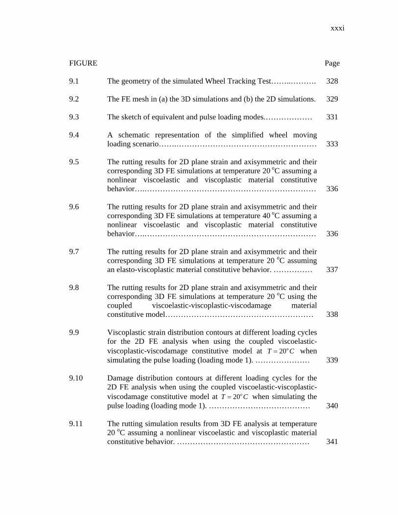
FIGURE Page 9.1 The geometry of the simulated Wheel Tracking Test……..………. 328 9.2 The FE mesh in (a) the 3D simulations and (b) the 2D simulations. 329 9.3 The sketch of equivalent and pulse loading modes.……………… 331 9.4 A schematic representation of the simplified wheel moving
loading scenario…….……………………………………………… 333 9.5 The rutting results for 2D plane strain and axisymmetric and their
corresponding 3D FE simulations at temperature 20 oC assuming a nonlinear viscoelastic and viscoplastic material constitutive behavior….………………………………………………………… 336
9.6 The rutting results for 2D plane strain and axisymmetric and their
corresponding 3D FE simulations at temperature 40 oC assuming a nonlinear viscoelastic and viscoplastic material constitutive behavior….………………………………………………………… 336
9.7 The rutting results for 2D plane strain and axisymmetric and their
corresponding 3D FE simulations at temperature 20 oC assuming an elasto-viscoplastic material constitutive behavior. …………… 337
9.8 The rutting results for 2D plane strain and axisymmetric and their
corresponding 3D FE simulations at temperature 20 oC using the coupled viscoelastic-viscoplastic-viscodamage material constitutive model………………………………………………… 338
9.9 Viscoplastic strain distribution contours at different loading cycles
for the 2D FE analysis when using the coupled viscoelastic-viscoplastic-viscodamage constitutive model at 20oT C when simulating the pulse loading (loading mode 1). ………………… 339
9.10 Damage distribution contours at different loading cycles for the
2D FE analysis when using the coupled viscoelastic-viscoplastic-viscodamage constitutive model at 20oT C when simulating the pulse loading (loading mode 1). ………………………………… 340
9.11 The rutting simulation results from 3D FE analysis at temperature
20 oC assuming a nonlinear viscoelastic and viscoplastic material constitutive behavior. …………………………………………… 341
xxxii
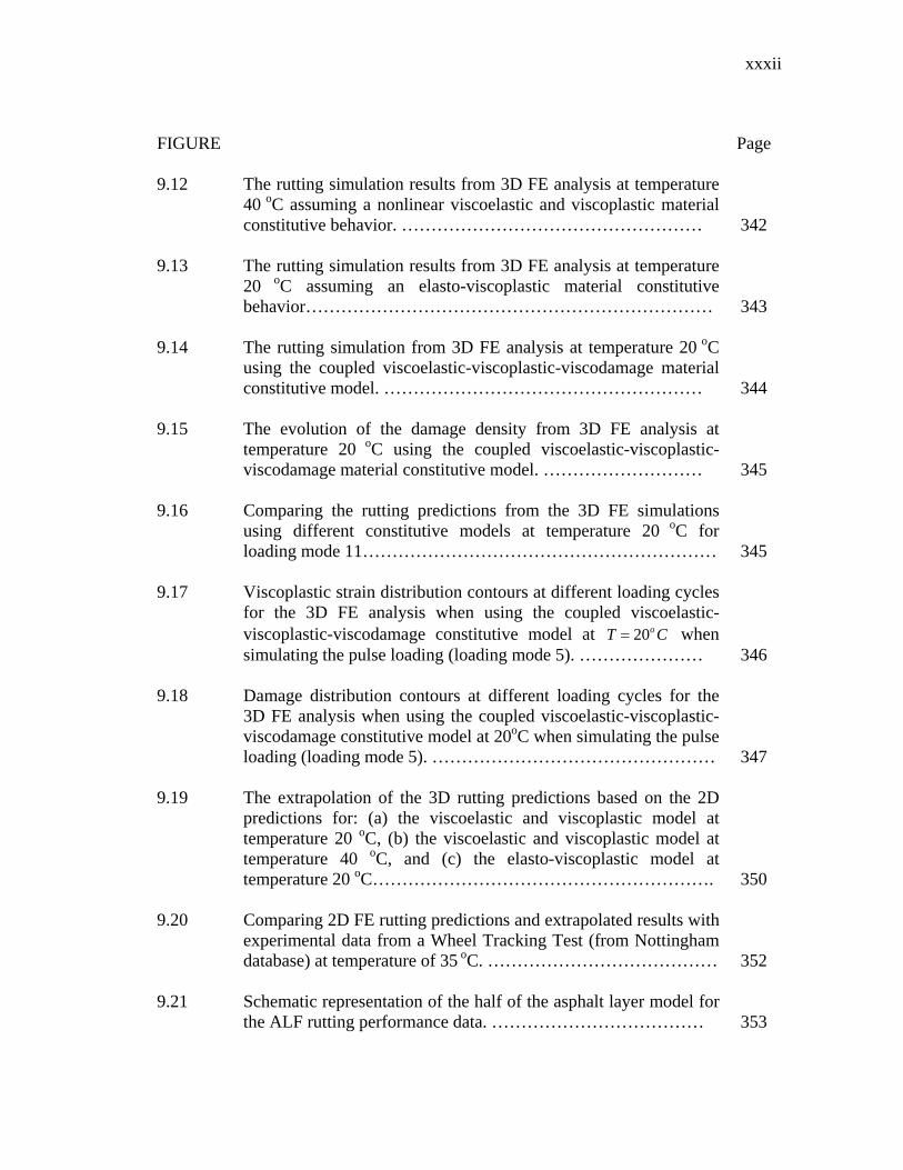
FIGURE Page 9.12 The rutting simulation results from 3D FE analysis at temperature
40 oC assuming a nonlinear viscoelastic and viscoplastic material constitutive behavior. …………………………………………… 342
9.13 The rutting simulation results from 3D FE analysis at temperature
20 oC assuming an elasto-viscoplastic material constitutive behavior…………………………………………………………… 343
9.14 The rutting simulation from 3D FE analysis at temperature 20 oC
using the coupled viscoelastic-viscoplastic-viscodamage material constitutive model. ……………………………………………… 344
9.15 The evolution of the damage density from 3D FE analysis at
temperature 20 oC using the coupled viscoelastic-viscoplastic-viscodamage material constitutive model. ……………………… 345
9.16 Comparing the rutting predictions from the 3D FE simulations
using different constitutive models at temperature 20 oC for loading mode 11…………………………………………………… 345
9.17 Viscoplastic strain distribution contours at different loading cycles
for the 3D FE analysis when using the coupled viscoelastic-viscoplastic-viscodamage constitutive model at 20oT C when simulating the pulse loading (loading mode 5). ………………… 346
9.18 Damage distribution contours at different loading cycles for the
3D FE analysis when using the coupled viscoelastic-viscoplastic-viscodamage constitutive model at 20oC when simulating the pulse loading (loading mode 5). ………………………………………… 347
9.19 The extrapolation of the 3D rutting predictions based on the 2D
predictions for: (a) the viscoelastic and viscoplastic model at temperature 20 oC, (b) the viscoelastic and viscoplastic model at temperature 40 oC, and (c) the elasto-viscoplastic model at temperature 20 oC…………………………………………………. 350
9.20 Comparing 2D FE rutting predictions and extrapolated results with
experimental data from a Wheel Tracking Test (from Nottingham database) at temperature of 35 oC. ………………………………… 352
9.21 Schematic representation of the half of the asphalt layer model for
the ALF rutting performance data. ……………………………… 353

xxxiii
FIGURE Page 9.22 Experimental measurements and model predictions of the rutting
performance for the ALF data. …………………………………… 353

xxxiv
LIST OF TABLES
TABLE Page 2.1 The summary of the tests used to identify the model parameters… 44 2.2 The identified viscoelastic-viscoplastic-viscodamage model
parameters at the reference temperature………………………… 51 2.3 Temperature coupling term model parameters [Eqs. (2.90) and
(2.91)] …………………………………………………………… 56 2.4 The summary of the tests used for validating the model………… 58 4.1 Model parameters associated with the presented elastic-damage-
healing constitutive model………………………………………… 128 7.1 Summary of the test used for identification of the thermo-
viscoelastic-viscoplastic model parameters……………………… 222 7.2 Identified viscoelastic model parameters at 0 10oT C and the time-
temperature model parameters. ………………………………….. 224 7.3 Viscoplastic model parameters at the reference temperature
0 10oT C . (Note that these parameters are obtained using the viscoplastic parameters identified at 55oC and the time-temperature shift factor identified from dynamic modulus test). … 227
7.4 Identified viscoplastic softening model parameters. ……………… 232 7.5 Summary of the test used for validation of the viscoelastic-
viscoplastic model with viscoplastic softening model. …………… 234 7.6 Summary of the tests in tension used for identification of the
thermo-viscodamage model parameters. ………………………… 246 7.7 Summary of the tests in tension used for validation of the thermo-
viscoelastic-viscoplastic-viscodamage-model.…...……………… 246

xxxv
TABLE Page 7.8 Viscodamage model parameters at the reference temperature
0 10oT C . (Note that these parameters are obtained using the viscodamage parameters identified at 5oC and the time-temperature shift factor identified from dynamic modulus test).… 257
9.1 Summary of simulated loading assumptions. …………………… 325 9.2 Assumed viscodamage model parameters for inducing early
damage growth. …………………………………………………… 334

1
CHAPTER I
INTRODUCTION AND LITERATURE REVIEW
1.1. Problem Statement
Asphalt concrete pavements are one of the largest infrastructure assets in the United
States and almost in every other country in the world. Although pavement design has
gradually moved from art to science, empirical relations and equations still play a
substantial role in design guides and manuals. The complex behavior of the constituents
of the pavements along with the environmental effects that pavements experience during
their service life has made it extremely difficult to develop fully mechanistic models to
predict the performance of pavements during their service life.
Various types of tests and models have been used to characterize the mechanical
response of asphalt concrete mixes as one of the main constituents of the pavements.
However, most of these models are developed to predict the responses under specific test
conditions or design problem, and therefore, are usually ad hoc and do not represent the
behavior of these materials under general three dimensional stress states and realistic
environmental conditions that actually happens in the field. The reason is that the asphalt
concrete mixes show nonlinear responses under different loading conditions.
Asphalt concrete mix and Hot Mix Asphalt (HMA) can be considered to be
consist of three scales :(a) the micro-scale (mastic), where fine fillers are surrounded by
the asphalt binder; (b) the meso-scale, fine aggregate mixture (FAM), where fine
aggregates are surrounded by the mastic; and (c) the macro-scale which includes all the
coarse aggregates surrounded by FAM. The complex interactions between these scales
are the primary source of nonlinearity in asphalt concrete mixes. Numerous experimental
studies have shown that the HMA response is time-, rate-, and temperature-dependent.
Several degree of magnitude of differences between the stiffness of the aggregate and
the binder makes the strain localization in the binder a dominant reason for the nonlinear
behavior of asphalt concrete mixes. Rotation and slippage of aggregates and interaction
between binder and aggregates during the loading are also other factors contributing to
This dissertation follows the style of International Journal of Plasticity.

2
the nonlinear behavior of asphalt concrete mixes. Moreover, the severe temperature
sensitivity of asphalt concrete mixes results in substantial changes of the behavior with
the temperature change. The combined effect of these phenomena causes the asphalt
mixes to show nonlinear responses even at very small strain or stress levels.
Added to this, the evolution of the permanent deformation in asphalt mixes
makes the mechanical response of these materials more nonlinear which is also a source
of a major distress in asphalt pavements referred to as rutting. Figure 1.1 shows a picture
of the severe rutting in an asphalt pavement section as a result of evolution of the
permanent deformation.
Figure 1.1. Rutting in the asphalt pavements as a result of evolution of the viscoplastic strain. This section is related to US 287 highway in Whichita Falls near Dallas Fort Worth.
Another major source of nonlinearity in the thermo-mechanical response of
HMA is the evolution of micro-cracks and micro-voids and rate-dependent plastic
(viscoplastic) hardening/softening. Figure 1.2 shows X-Ray computed tomography (CT)
images of the cross-section of an asphalt mixture laboratory specimen before loading
and at different strain levels. As it is shown in Figure 1.2 (b)-(d), micro-damages (micro-
cracks and micro-voids) nucleate and propagate progressively as the material deforms
and cause the stiffness to degrade. However, at specific temperature ranges, the binder in

3
the asphalt mixes and subsequently the asphalt concrete mix has the potential to heal
with time and recover part of its strength and stiffness during the rest period. Therefore,
an accurate prediction of the thermo-mechanical response of asphalt mixes and
bituminous materials require the coupling between viscoelasticty, viscoplasticity,
viscodamage, and healing models.
Figure 1.2. X-Ray images of the cross-section of an asphalt mixture laboratory specimen
subjected to triaxial loading. (a) Before loading; (b) 2% strain; (c) 4% strain; (d) 8% strain. Micro-damages (i.e. micro-cracks and micro-voids) nucleate and propagate as the material
deforms.
In addition to thermo-mechanical loadings, pavements are subjected to
environmental conditions such as moisture and oxygen. The moisture at the surface of
the asphalt mixes in the forms of water or environmental humidity disperses into the
mixture, fully/partially fills the air voids, and diffuses to the solid part through the
diffusion process. The infiltrated moisture may yield to stiffness and strength
degradation because of chemical, physical, and mechanical processes. This effect is
referred to as moisture damage in this work and may cause the aggregates in the asphalt

4
surface to loosen gradually and separate individually from the asphalt layer. On the other
hand, the existing oxygen in the air in contact with the asphalt layer of a pavement can
also diffuse inside the asphalt layer through the interconnected air voids. Once infiltrated
by oxygen, the binder phase in the mix reacts with oxygen resulting in changes in the
mechanical properties of asphalt concrete mixes. This phenomenon is known as aging
which is the result of the chemical reaction of oxygen with binder.
More complication arises because each individual processes (i.e. thermo-
viscoelasticity, thermo-viscoplasticity, thermo-viscodamage, healing, moisture damage,
and aging) also interact with one another and are in most cases coupled. For instance,
crack propagation enables more water and higher amount of oxygen to diffuse inside the
mix and accelerates the moisture damage and aging effects. It also yields to the
acceleration of accumulative permanent deformation in the mix. Subsequently, the
increase in the deformation causes more damage growth which degrades the mechanical
properties of the mix in higher extent which obviously makes the mix to be more prone
to distresses. This process is very important in predicting the performance prediction of
asphalt pavements.
The presence of different mechanical, thermal, and environmental effects in the
pavements during their service life makes it necessary to develop a robust constitutive
model to predict the multi-physics response of asphalt mixes in the pavements.
However, the developed constitutive model should be as general as possible and be
validated over extensive experimental measurements to ensure proper model response
under complex three-dimensional stress states. In fact, development of such constitutive
models for a specific material has been the main challenge of the modern constitutive
modeling. This can be effectively achieved, so far, through the thermodynamic
principles by enforcing the balancing laws, the conservation of mass, the conservation of
linear and angular momentums, and the first and second laws of thermodynamics.
The ultimate goal of developing a robust constitutive model is to provide a
reliable tool for predicting the pavement performance during its service time. This raises
another challenging task which is the proper computational techniques for pavement

5
performance predictions. The long life of pavements, very large number of loading
cycles (millions of loading cycles), the complex constitutive model, and the complex
nature of the applied loading conditions make the development of an accurate and yet
affordable computational technique very difficult and challenging task. Even with the
current state-of-the-art in computational power, conducting realistic 3D finite element
(FE) rutting and/or fatigue performance simulations for pavements subjected to millions
of wheel loading cycles by considering realistic wheel/pavement interactions and
environmental effects is almost impossible.
Added to the mentioned challenges in developing computational techniques,
strain and damage localization phenomena in the asphalt concrete mixes causes
instabilities and mesh-dependent results in the FE simulations. In other words, as the
loading increases, asphalt binder undergoes a substantial strain levels comparing to the
applied strain to the HMA. For example, strain in the binder could range between
average of eight times and a maximum of 510 times the bulk strain of the mixture (Kose
et al., 2000) and some regions within the mastic can experienced strain levels as high as
30 times the applied strain (Masad and Somadevan, 2002). These localizations lead to
the mesh-dependent results in the FE simulations specially at softening regions such that
the traditional local continuum theories fail to predict physical response. One alternative
to remedy this problem is to use and implement non-classical gradient-dependent
continuum theories.
This work tries to contribute in filling the gap in constitutive modeling and
computational techniques of bituminous materials and asphalt mixes. Therefore, a
thermo-viscoelastic-viscoplastic-viscodamage-healing constitutive model is developed to
model the complex response of these materials under more realistic conditions. The term
“visco” is referred to time- and rate-dependent characteristic of the model, whereas, the
term “thermo” is related to temperature-dependent response of bituminous materials.
The developed model is calibrated, validated, and subsequently implemented in the well-
known finite element code Abaqus (2008) through the user material subroutine UMAT.

6
The implemented model is finally used to predict the complex mechanical response of
asphalt mixes and to conduct the performance simulation of asphalt pavements.
1.2. Background and State of the Art
Numerous experimental studies on polymers, bituminous materials, asphalt
mixes, and soft materials have shown that the mechanical response of these materials is
time- and rate-dependent. These materials clearly display all four fundamental
mechanical responses (i.e. viscoelasticity, viscoplasticity, viscodamage, and healing)
where contribution of each response strongly depends on the temperature and loading
conditions. For example, the viscoelastic response could be dominant at low
temperatures and stress levels, whereas viscoelastic and viscoplastic responses are
dominant at high temperatures. However, the viscodamage (rate-dependent damage)
response becomes very important at post peak stress-strain regions, high stress levels,
and long loading periods; whereas for some materials, the healing could be significant in
fatigue loadings. This section provides the background and a limited literature review on
the modeling efforts to simulate these effects. These previous works are considered as
the foundation for developing new theories and modifying the existing ones for each
component of the thermo-viscoelastic-viscoplastic-viscodamage-healing model proposed
in this work.
1.2.1. Viscoelasticity
Experimental observations have clearly shown that the response of asphalt mixes
show both recoverable and irrecoverable components (Perl et al., 1983; Collop et al.,
2003; Huang, 2008). The recoverable component is usually modeled using the solid-like
viscoelasticity models, whereas, the irrecoverable component is usually modeled using
fluid-like viscoelasticity and/or viscoplasticity models.
In terms of the viscoelastic behavior of materials, Biot (1954) derived a
formulation for linear viscoelastic materials. Schapery (1969b) used the thermodynamics
of irreversible processes and developed a single integral constitutive model for nonlinear
viscoelastic materials such as polymers (e.g. Christen, 1968; Schapery, 1969a, b; Sadkin

7
and Aboudi, 1989; Haj-Ali and Muliana, 2004; Muliana and Haj-Ali, 2008). Schapery’s
constitutive model has been applied to asphalt mixes by several other researchers (e.g.
Huang et al., 2007; Masad et al., 2008; Abu Al-Rub et al., 2009; Saadeh and Masad,
2010; Darabi et al., 2011c). Moreover, Touti and Cederbaum (1998), Haj-Ali and
Muliana (2004), Sadd et al. (2003), and Huang et al. (2007) developed algorithms for
numerical implementation of Schapery’s viscoelastic constitutive model in finite element
codes. Recently, Levesque et al. (2008) extended the Schapery’s nonlinear viscoelastic
model for 3D applications based on laws of thermodynamics. Masad et al. (2009), Abu
Al-Rub et al. (2010a), Huang et al. (2011a), and Darabi et al. (2011c) have developed
and applied a systematic procedure to characterize and decouple the recoverable
(viscoelastic) by analyzing repeated creep-recovery experimental tests using Schapery’s
nonlinear viscoelastic model.
These studies clearly show that the viscoelastic response of HMA can be well-
predicted using Schapery’s nonlinear viscoelasticity model (Huang et al., 2007; Masad et
al., 2008; Abu Al-Rub et al., 2010a; Darabi et al., 2011c). It should be noted that the
Schapery’s linear/nonlinear model is a solid-like viscoelastic model and predicts only the
recoverable strains.
1.2.2. Viscoplasticity
Two approaches have been used in the literature to model the irrecoverable
component of the deformation in bituminous materials and asphalt mixes. The first
approach is based on the spring-dashpot analogy and development of fluid-like
viscoelasticity models; whereas, the second approach is to use the plastic/viscoplastic
models to represent the irrecoverable component of the strain and deformation.
One of the early models for describing the mechanical behavior of bituminous
materials is the burger’s model (Burgers, 1939) which has also been used and modified
by Saal and Labout (1940). Krishnan and Rajagopal (2004, 2005) introduced the concept
of the natural configurations and derived a large deformation fluid-like viscoelasticity
theory based on the spring-dashpot analogy to predict the mechanical response of
asphalt. However, they assumed the incompressibility condition which has not been fully
8
validated experimentally. In fact, the experimental measurements on the asphalt concrete
show the development of significant volumetric strains in deformation (Erkens, 2002). In
another attempt, Scarpas, Kringos and their co-workers at Delft University of
Technology derived a large deformation viscoplasticity theory using the concept of
spring-dashpot analogy (e.g. Scarpas, 2004; Kringos et al., 2007; Kringos et al., 2010).
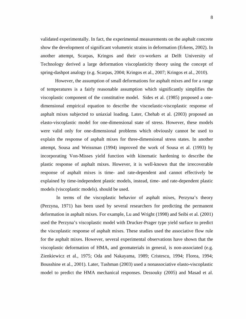
However, the assumption of small deformations for asphalt mixes and for a range
of temperatures is a fairly reasonable assumption which significantly simplifies the
viscoplastic component of the constitutive model. Sides et al. (1985) proposed a one-
dimensional empirical equation to describe the viscoelastic-viscoplastic response of
asphalt mixes subjected to uniaxial loading. Later, Chehab et al. (2003) proposed an
elasto-viscoplastic model for one-dimensional state of stress. However, these models
were valid only for one-dimensional problems which obviously cannot be used to
explain the response of asphalt mixes for three-dimensional stress states. In another
attempt, Sousa and Weissman (1994) improved the work of Sousa et al. (1993) by
incorporating Von-Misses yield function with kinematic hardening to describe the
plastic response of asphalt mixes. However, it is well-known that the irrecoverable
response of asphalt mixes is time- and rate-dependent and cannot effectively be
explained by time-independent plastic models, instead, time- and rate-dependent plastic
models (viscoplastic models). should be used.
In terms of the viscoplastic behavior of asphalt mixes, Perzyna’s theory
(Perzyna, 1971) has been used by several researchers for predicting the permanent
deformation in asphalt mixes. For example, Lu and Wright (1998) and Seibi et al. (2001)
used the Perzyna’s viscoplastic model with Drucker-Prager type yield surface to predict
the viscoplastic response of asphalt mixes. These studies used the associative flow rule
for the asphalt mixes. However, several experimental observations have shown that the
viscoplastic deformation of HMA, and geomaterials in general, is non-associated (e.g.
Zienkiewicz et al., 1975; Oda and Nakayama, 1989; Cristescu, 1994; Florea, 1994;
Bousshine et al., 2001). Later, Tashman (2003) used a nonassociative elasto-viscoplastic
model to predict the HMA mechanical responses. Dessouky (2005) and Masad et al.

9
(2007), extended the work of Tashman (2003) by modifying the yield surface to
distinguish between the viscoplastic behavior in compression and extension state of
loading. However, they also used the time-independent elastic models for the
recoverable component of the deformation which is not the case for asphalt mixes.
Saadeh et al. (2007), Huang (2008), Abu Al-Rub et al. (2009; 2010a), Darabi et al.
(2011c), and Huang et al. (2011a) coupled the nonlinear viscoelasticity model of
Schapery and Perzyna’s viscoplasticity model to simulate more accurately the nonlinear
mechanical response of HMA at high stress levels and high temperatures.
1.2.3. Viscodamage
The coupled viscoelastic-viscoplastic constitutive models yield reasonable predictions of
the mechanical response of asphalt mixes prior to the damage. However, the changes in
the material’s microstructure during deformation cause HMA materials to experience a
significant amount of micro-damage (micro-cracks and micro-voids) under service
loading conditions, where specific phenomena such as tertiary creep, post-peak behavior
of the stress-strain response, and degradation in the mechanical properties of HMA is
mostly due to damage and cannot be explained only by viscoelasticity and
viscoplasticity constitutive models.
Models based on the continuum damage mechanics (CDM) have been effectively
used to model the degradations in materials due to cracks and voids (Kachanov, 1958;
Rabotnov, 1969; Fanella and Krajcinovic, 1985; Voyiadjis and Kattan, 1992; Lemaître,
1996; Voyiadjis and Thiagarajan, 1997). Masad et al. (2005) included isotropic (scalar)
damage in an elasto-viscoplastic model (modified by Saadeh et al. (2007), Graham
(2009), and Saadeh and Masad (2010) to include Schapery’s nonlinear viscoelasticity) to
simulate the mechanical response of asphalt mixes. Another attempt is made by Uzan
(2005) to develop a damage-viscoelastic-viscoplastic model for asphalt mixes, but this
model is valid for one-dimensional problems and cannot be used for multi-axial state of
stresses. Moreover, in most of these works the damage laws are not time- and rate-
dependent which is a challenge in the modeling of asphalt mixes. This argument is
experimentally motivated since various experimental studies have shown that the

10
damage response of bituminous materials depends on temperature, time, and rate of
loading (Kim and Little, 1990; Collop et al., 2003; Masad et al., 2007). Several rate-
dependent damage models (usually referred to as the creep-damage laws) have been
proposed in the literature. Kachanov (1958), Odqvist and Hult (1961), and Rabotnov
(1969) pioneered in proposing the creep-damage evolution laws. Later, various types of
creep-damage laws in terms of stress, strain, and energy have been proposed by other
researchers (Cozzarelli and Bernasconi, 1981; Lee et al., 1986; Voyiadjis et al., 2004;
Abu Al-Rub and Voyiadjis, 2005b; Zolochevsky and Voyiadjis, 2005). Although many
papers are devoted to improve the damage evolution laws in elastic media (Kachanov,
1986; Lemaître, 1992; Krajcinovic, 1996; Lemaître and Desmorat, 2005), very few
damage models have been coupled to viscoelasticity and viscoplasticity in order to
predict the mechanical response of time- and rate-dependent materials. In fact, there are
few studies that couple damage to viscoelasticity to include time and rate effects on
damage evolution laws (Schapery, 1975c; Schapery, 1975a, b; Simo, 1987; Weitsman,
1988; Gazonas, 1993; Sullivan, 2008). Schapery’s viscoelastic-damage model
(Schapery, 1975b; Schapery, 1987), which has been modified by Schapery (1999) to
include viscoplasticity, is currently used to reasonably predict the damage behavior of
asphaltic materials (Kim and Little, 1990; Park et al., 1996; Gibson et al., 2003; Kim et
al., 2007). This model is based on the elastic-viscoelastic correspondence principle that
is based on the pseudo strain for modeling the linear viscoelastic behavior of the
material; the continuum damage mechanics based on pseudo strain energy density for
modeling the damage evolution; and time-temperature superposition principle for
including time, rate, and temperature effects. However, it has the following limitations:
(1) it can be used only to predict viscoplasticity and damage evolution in tensile loading
conditions; and (2) it treats asphaltic materials as linear viscoelastic materials
irrespective of temperature and stress levels. Recently, Darabi et al. (2011c) proposed a
phenomenological temperature-dependent viscodamage model and coupled it to
Schapery’s viscoelasticity and Perzyna’s viscoplasticity in order to realistically model
the mechanical responses of asphalt mixes.

11
1.2.4. Micro-Damage Healing
Experimental observations in the last few decades have clearly shown that
various classes of engineering materials (e.g. polymers, bitumen, bio-inspired materials,
rocks) have the potential to heal with time and recover part of their strength and stiffness
under specific circumstances (e.g. Miao et al., 1995; Kessler and White, 2001; Brown et
al., 2002; Reinhardt and Jooss, 2003; Guo and Guo, 2006; Kessler, 2007; Bhasin et al.,
2008). Constitutive models that do not account for healing of these materials
significantly underestimate their fatigue life that will lead to very conservative design of
structural systems made of such materials. Therefore, it is imperative to model healing
for more accurate fatigue life predictions.
Changes in the material’s microstructure during deformation usually cause
significant micro-damage (micro-cracks and micro-voids) under service loading
conditions. The creation and coalescence of micro-damages lead to degradation in the
material’s mechanical properties including strength and stiffness. This process of
degradation can progressively continue up to complete failure. Theories based on
continuum damage mechanics have been successfully used to explain these degradation
in different materials.
However, a common assumption in the theories based on continuum damage
mechanics is that the damage process is irreversible (e.g. Kachanov, 1958, 1986;
Lemaître and Chaboche, 1990; Lemaître, 1992; Voyiadjis and Kattan, 1992; Kattan and
Voyiadjis, 1993; Krajcinovic, 1996; Voyiadjis and Park, 1999; Voyiadjis and Deliktas,
2000; Lemaître, 2002; Abu Al-Rub and Voyiadjis, 2003, 2005b; Voyadjis and Abu Al-
Rub, 2006). In other words, the damage variable is usually assumed to be a
monotonically increasing function. However, during the unloading process and resting
time periods some micro-crack and micro-void free surfaces wet and are brought back
into contact with one another. In certain materials such as polymers and especially
asphalt mixes, micro-cracks and micro-voids gradually reduce in size with a
corresponding recovery in strength and stiffness due to micromechanical short-term
wetting and long-term diffusion processes as the resting period increases (Wool and

12
Oconnor, 1981). These healing features are opposite to those normally associated with
continuum damage mechanics. In fact, for long resting periods, the damaged area may
recover all of its strength and becomes identical to the virgin state of material (Prager
and Tirrell, 1981; Carpenter and Shen, 2006; Little and Bhasin, 2007). This process is
referred to as micro-damage healing.
The importance of the micro-damage healing process depends on loading
conditions. For example, the result of the healing process can be significant when the
material is subjected to fatigue loading conditions where rest time periods are introduced
between the loading cycles. This is the case in asphaltic pavements under traffic loading
conditions (Kim and Little, 1989; Lytton et al., 1993; Kim et al., 1994; Si et al., 2002).
In other words, the impact of the recovery process is cumulative and depends on
variables such as the length of the rest period and the temperature of the asphalt mixture.
Moreover, Shen and Carpenter (2005), Carpenter and Shen (2006), and Shen et al.
(2006) have documented the efficacy of the dissipated energy approach to fatigue
damage as well as the cumulative impact of healing even for very short rest periods
during the fatigue damage process. Furthermore, Zhang et al. (2001b) and Kim and
Roque (2006) have identified the importance of considering a healing property in fatigue
damage and the crack growth process. In another work, Zhang et al. (2001a) introduced
the concept of a threshold fracture energy density as a failure criterion for the initiation
and propagation of cracks. They state that at the “local level, in front of the crack tip, or
in areas of high stress concentration, one could use the fracture energy density as a
criterion below which cracks will not initiate or propagate”. This is a pertinent
observation with regard to healing as this study focuses on the importance of considering
the recovery of damage in the area that precedes the crack tip during the healing process.
Several micromechanical- and phenomenological-based models for predicting
micro-damage healing in different materials have been proposed (Wool and Oconnor,
1981; Schapery, 1989; Miao et al., 1995; Jacobsen et al., 1996; Ramm and Biscoping,
1998; Ando et al., 2002; Little and Bhasin, 2007). Wool and O’connor (1981) proposed
a phenomenological-based theory of crack healing in polymers and introduced a
13
macroscopic recovery parameter that is the convolution of an intrinsic healing function
and the rate of wetting distribution function to relate the healing at micro scale to the
changes in the mechanical properties of polymers at the macro scale. Schapery (1989)
proposed a fracture mechanics-based model to describe the rate of crack shortening for
linear viscoelastic materials using the correspondence principle. Miao et al. (1995)
presented a thermodynamic-based model for healing of crushed rock salt. Little and
Bhasin (2007) and Bhasin et al. (2008) combined the contributions of Wool and
O’connor (1981) with those of Schapery (1989) and defined a macroscopic recovery
parameter to quantify healing in bituminous materials. They showed that the rest period
have a significant effect on healing.
However, these models are mostly: (1) micromechanical- and fracture
mechanics-based that cannot be easily used at the macroscopic level to solve an
engineering problem; (2) augmented with several material parameters that are difficult to
identify based on available macroscopic experiments; (3) usually developed for specific
loading conditions and cannot be used for capturing healing effects under different
loading conditions; and (4) not coupled with the viscoelastic, viscoplastic, and/or
damage constitutive behavior of the healed material. Hence, development of a general
and robust healing model at the continuum level seems appropriate and necessary as a
contribution to understanding and modeling the general fatigue damage process.
Surprisingly, little attention is devoted to the development of such a healing model and
its coupling to the visco-inelastic response of asphaltic materials.
It is noteworthy that the problem of viscoelastic, viscoplastic, damage, and
healing in bituminous materials and specially asphalt mixes is very complicated.
Therefore, a rigorous thermodynamic basis for modeling the viscoelastic, viscoplastic,
damage, and healing mechanisms should be developed in order to explain how these
mechanisms store energy and how each of these mechanisms affect the entropy
production. Rajagopal and his co-workers have presented a rigorous thermodynamic-
based model to explain the viscoelastic response of asphalt mixes (e.g. Krishnan and
Rajagopal, 2003; Krishnan and Rajagopal, 2004; Koneru et al., 2008; Ravindran et al.,

14
2009 and the references quoted therein). The procedure for the development of
thermodynamically consistent coupled viscoelastic-viscoplastic-viscodamage-healing
constitutive model will be presented in the next chapters of this work.
Moreover, asphalt mixture is a highly complex material which is a mixture of
asphalt binder, aggregate, and air voids. The properties of these constituents have
significant effect on the overall property of asphalt mixture. Mixture theory is one of the
modern techniques to model the behavior of different mixtures such as asphalt mixtures
initially proposed for modeling the mixture behavior of fluids (Ingram and Cemal
Eringen, 1967; Truesdell, 1969). However, one of the important problems in using the
mixture theories is how to handle the boundary condition problem between different
constituents (c.f. Rajagopal and Tao, 1996; Krishnan and Rao, 2000). These theories
along with the framework of natural configurations (Rajagopal and Wineman, 1992;
Rajagopal, 1995) have been used by several researchers to explain the mechanical
properties of asphalt mixtures (e.g. Krishnan and Rao, 2000; Krishnan and Rajagopal,
2003; Krishnan and Rajagopal, 2004; Wang et al., 2004; Koneru et al., 2008; Ravindran
et al., 2009). Although using the mixture theory is one of the promising approaches for
modeling the behavior of asphalt mixes, they are augmented with several model
parameters at the mixture level and for each of the constituents. Hence, in this paper we
consider a single homogenized continuum approach to model the mechanical response of
asphalt mixes.
1.3. Scope and Objective
The main objective of this work is to develop a thermo-viscoelastic-viscoplastic-
viscodamage-healing constitutive model and to apply it for predicting the response of
bituminous materials, asphalt mixes, and pavements under realistic mechanical
conditions. This objective is achieved through the following tasks:
1- Development of a time-, rate-, and temperature-dependent damage model
(thermo-viscodamage) and couple it with thermo-viscoelastic and thermo-
viscoplastic models.

15
2- Development of a general framework to model the micro-damage healing in
materials with the healing capability.
3- Development of a micro-damage healing model for asphalt mixes for more
accurate prediction of the response under cyclic loading conditions.
4- Development of a general thermodynamic framework that provides a
systematic procedure for deriving thermodynamically consistent constitutive
models.
5- Implementing the proposed thermo-mechanical constitutive model in the
finite element (FE) codes.
6- Validating the constitutive model and subsequently applying it for
performance prediction of the pavements.
1.4. Organization of the Dissertation
This dissertation is organized following the research paper format. Chapters II,
III, IV, V, VI, VII, VIII, and IX are research papers that have been or will be submitted
as refereed journal papers.
Chapter I includes the introduction which contains background on modeling
asphalt mixture response and performance, problem statement, objectives and the outline
of this dissertation. Chapter II presents the development of a thermo-viscoelastic-
viscoplatic-viscodamage model for asphaltic materials. Chapter III proposes a
thermodynamic-based framework to ensure the consistency of the proposed model.
Chapter IV introduces a continuum damage mechanics framework for modeling the
micro-damage healing in materials and Chapter V proposes a micro-damage healing
model for asphalt mixes. Chapter VI proposes a general thermodynamic-based
framework for constitutive modeling of time- and rate-dependent materials. The
proposed thermo-mechanical model is validated against another extensive experimental
measurements in Chapter VII. Chapter VIII develops a numerical technique for
implementation of the gradient-dependent continuum damage mechanics theories and
the model is used to conduct the performance simulation of asphalt pavements in

16
Chapter IX. Final conclusions, recommendations, and future works are presented in
Chapter X.

17
CHAPTER II
A THERMO-VISCOELASTIC-VISCOPLASTIC-VISCODAMAGE
MODEL FOR ASPHALTIC MATERIALS
2.1. Introduction
Because of the complex behavior of HMA, the coupling of the nonlinear thermo-
viscoelasticity, thermo-viscoplasticity, and temperature- and rate-dependent damage
(thermo-viscodamage) modeling seems inevitable. However, surprisingly, very limited
work has been focusing on the development of such models, and the current study
attempts to close this gap and develops a robust model that overcomes the limitations of
the current models for HMA. This chapter proposes a temperature dependent
viscodamage model which is coupled to nonlinear temperature-dependent Schapery’s
viscoelastic model (Schapery, 1969a) and temperature-dependent Perzyna’s
viscoplasticity model (Perzyna, 1971) to model the nonlinear constitutive behavior of
asphalt mixes. The viscodamage model is formulated to be a function of temperature,
total effective strain, and the damage driving force which is expressed in terms of the
stress invariants of the effective stress in the undamaged (effective) configuration.
However, it is well-recognized that the damage response of asphalt mixes is
different in compression and extension state of loading. Therefore, the damage driving
force is formulated such that it allows for the distinction between the influence of
compression and extension loading conditions on damage nucleation and growth. A
systematic procedure is presented to identify temperature-dependent viscoelasticity,
viscoplasticity, and viscodamage model parameters. The viscoelastic model parameters
are identified by extracting the pure viscoelastic response during the recovery part of the
creep-recovery test (Huang, 2008). Subsequently, the viscoplastic response during the
creep part of the creep-recovery test is obtained by subtracting the viscoelastic strain
from the total strain. This response is then used to identify the viscoplastic model
parameters (Abu Al-Rub et al., 2009; Huang et al., 2011a). Finally, the viscodamage
model parameters are identified from two creep tests that show the secondary and
18
tertiary responses (Darabi et al., 2011c). The presented model is implemented in the
well-known finite element code Abaqus (2008) through the user subroutine UMAT to
validate the model over the experimental data which was not used in the calibration
process. The recursive-iterative and radial return algorithms are used for the numerical
implementation of the nonlinear viscoelasticity and viscoplasticity models, respectively,
whereas the viscodamage model is implemented using the effective (undamaged)
configuration concept. It is shown that the presented constitutive model is capable of
predicting the nonlinear behavior of asphaltic mixes under different loading conditions.
2.2. Total Strain Additive Decomposition
The total deformation of the Hot Mix Asphalt (HMA) subjected to an applied stress can
be decomposed into recoverable and irrecoverable components, where the extent of each
is mainly affected by time, temperature, and loading rate. In this study, small
deformations are assumed such that the total strain is additively decomposed into a
viscoelastic (recoverable) component and a viscoplastic (irrecoverable) component:
nve vpij ij ij (2.1)
where ij is the total strain tensor, nveij is the nonlinear viscoelastic strain tensor, and vp
ij
is the viscoplastic strain tensor. The constitutive equations necessary for calculating nveij
and vpij will be presented in the following sections.
2.3. Effective (Undamaged) Stress Concept
Kachanov (1958) has pioneered the concept of continuum damage mechanics (CDM),
where he introduced a scalar measure called continuity, , which is physically defined
by Rabotnov (1969) as:
A
A (2.2)
where A is the damaged (apparent) area and A is the real area (intact or undamaged
area) carrying the load. In other words, A is the resulted effective area after micro-

19
damages (micro-cracks and micro-voids) are removed from the damaged area A . The
continuity parameter has, thus, values ranging from 1 for intact (undamaged)
material to 0 indicating total rupture.
Odqvist and Hult (1961) introduced another variable, , defining the reduction
of area because of the micro-damages:
1DA A A
A A (2.3)
where DA is the area of micro-damages such that DA A A . is the so-called
damage variable or damage density which can be interpreted as the density of micro-
damages (micro-cracks and micro-voids) with values ranging from 0 (undamaged) to 1
(complete damage). In fact, fracture or complete rupture mostly occurs when c ,
where c is the critical damage density, which is a material property (Abu Al-Rub and
Voyiadjis, 2003). In this study, isotropic damage is assumed such that the stress tensor
components are degraded equally in different directions.
Based on CDM definition of an effective area, the relationship between stresses
in the undamaged (effective) material and the damaged material is defined as [see
Chaboche (2003) for a concise review of effective stress in CDM]:
1
ijij
(2.4)
where is the effective stress tensor in the effective (undamaged) configuration and
is the nominal Cauchy stress tensor in the nominal (damaged) configuration. The
schematic representation of the nominal (damaged) and effective (undamaged)
configurations is shown in Figure 2.1.

20
Figure 2.1. Schematic representation of the effective and nominal configurations.
It is noteworthy that the effective stress is the one that drives viscoelastic and
viscoplastic deformations. Moreover, it is usually argued that once the material is
damaged, further loading can only affect the undamaged material skeleton. Hence, the
viscoelastic, viscoplastic, and viscodamage models are defined as functions of variables
in the effective configuration. The superimposed “” in this work designates the
effective configuration.
However, a transformation hypothesis is required to relate the nominal stress and
strain tensors ( and ) to the stress and strain tensors in the undamaged configuration
( and ). For this purpose, one can either adapt the strain equivalence hypothesis (i.e.
the strains in nominal and effective configurations are equal) or the strain energy
equivalence hypothesis (i.e. any form of strain energy in the nominal configuration is
equal to the corresponding strain energy in the effective configuration) [see Voyiadjis
and Kattan (1999) for more details].
Although, the strain energy equivalence hypothesis is intuitively more physically
sound, but greatly complicates the constitutive models and their numerical
implementation (Abu Al-Rub and Voyiadjis, 2003). Therefore, for simplicity and
easiness in the finite element implementation of the subsequent complex constitutive
equations, the strain equivalence hypothesis is adopted. Hence, one can assume that the
nominal strain tensors , nve , and vp are equal to their counterparts in the effective
configuration, , nve , and vp , such that:
Effective (undamaged) configuration
Nominal (damaged) configuration
Remove both voids and cracks

21
ij ij , nve nveij ij , vp vp
ij ij (2.5)
where nve and vp are the nonlinear viscoelastic and viscoplastic strain tensors in the
nominal configuration, respectively; whereas nve and vp are the nonlinear viscoelastic
and viscoplastic strain tensors in the effective configuration, respectively. This
transformation hypothesis makes the numerical implementation of constitutive equations
very easy and avoids the complexities associated with direct couplings between the
damage model and different parts of the constitutive model. In fact, for small
deformations and isotropic (scalar) damage assumptions, one can assume that the strain
differences in the nominal and effective configurations are negligible (Abu Al-Rub and
Voyiadjis, 2003), such that postulating the strain equivalence hypothesis seems
admissible. However, the strain equivalence hypothesis results in linear variation of the
stiffness modulus with the damage density which is not experimentally motivated. To
remedy this issue, Cicekli et al. (2007) and Abu Al-Rub and Voyiadjis (2009) modified
Eq. (2.4), such that:
2(1 )
ijij
(2.6)
Eq. (2.6) (which is used in this work) allows the quadratic variation of the damaged
stiffness with respect to the damage density when the strain equivalence hypothesis is
use.
It should be noted that the equivalency of the strain tensor in the effective and
nominal configuration is assumed here for simplicity and might not be an accurate
assumption for large deformation theories when damage is significant. In these cases,
one may use alternative approaches such as postulating the strain energy equivalence
hypothesis, power equivalence hypothesis, or taking into account the changes in the
density of the damaged materials by adapting finite deformation theories (c.f. Davison
and Stevens, 1973; Davison et al., 1977; Voyiadjis and Kattan, 1992; Lubarda and
Krajcinovic, 1995).

22
2.4. Nonlinear Thermo-Viscoelastic Model
In this study, the Schapery’s nonlinear viscoelasticity theory (Schapery, 1966) is used to
model the viscoelastic response of HMA. The Schapery’s viscoelastic one-dimensional
single integral model is expressed here in terms of the effective stress , Eq. (2.6), as
follows:
2,0 0 1 0
( , )( , ) ( , )
tnve t t t t t t td g T
g T D g T D dd
(2.7)
where 0D is the instantaneous compliance; D is the transient compliance; 0g , 1g , and
2g are nonlinear parameters related to the effective stress, , strain level, nve , or
temperature T at a specific time . The parameter 0g is the nonlinear instantaneous
compliance parameter that measures the reduction or the increase in the instantaneous
compliance. The transient nonlinear parameter 1g measures nonlinearity effects in the
transient compliance. The nonlinear parameter 2g accounts for the loading rate effect on
the creep response. Note that 0D , D , 0g , 1g , and 2g should be determined for
undamaged material. In Eq. (2.7), t is the reduced-time given by:
0
tt
T s e
d
a a a
(2.8)
where Ta , sa , and ea are the temperature, strain or stress, and environment (e.g.
moisture, aging) shift factors, respectively. It is noteworthy to mention assuming 0g , 1g ,
and 2g to be constant and equal to one simplified the Schapery’s nonlinear viscoelastic
model [Eq. (2.7)] to the Boltzmann superposition integral for linear viscoelastic
materials. For numerical convenience, the Prony series is used to represent the transient
compliance D , such that:
1
1 expt
Nt
n nn
D D
(2.9)

23
where N is the number of terms, nD is the thn coefficient of Prony series associated
with the thn retardation time n . In the above and subsequent equations, the
superimposed t and designate the response at a specific time.
As proposed by Lai and Bakker (1996), the one-dimensional nonlinear
viscoelastic model in Eq. (2.7) can be generalized to three-dimensional problems by
decoupling the response into deviatoric and volumetric parts, such that:
1 1
3 2 9 2 3ij
nve nve nve kkij kk ij ij ij ij kk ij
J Be S S
G K
(2.10)
where nvee and nvekk are the deviatoric strain tensor and the volumetric component of the
strain tensor, respectively; G and K are the undamaged shear and bulk moduli,
respectively, which are related to the undamaged Young’s modulus E and Poisson’s
ratio by:
/ 2(1 )G E , / 3 1 2K E (2.11)
J and B are the undamaged shear and bulk compliances, respectively;
/ 3ij ij kk ijS is the deviatoric stress tensor in the effective configuration; ij is the
Kronecker delta; and kk is the volumetric stress in the effective (undamaged)
configuration. Using Schapery’s integral constitutive model [Eq. (2.7)] and after some
mathematical manipulations, the deviatoric and volumetric components of the nonlinear
viscoelastic strain at time t can be expressed, respectively, as follows (Lai and Bakker,
1996):
2, ( )0 0 1
0
( )1 1
2 2
tt
ijnve t t t tij ij
d g Se g J S g J d
d
(2.12)
, ( ) 20 0 1
0
( )1 1
3 3
tt
nve t t t t kkkk kk
d gg B g B d
d
(2.13)
where the material constants 0J and 0B are the instantaneous effective elastic shear and
bulk compliances, respectively. The Poisson’s ratio is assumed to be time-
independent which is a fairly reasonable assumption for a range of temperatures and

24
stress rates in the asphaltic materials (e.g. Di Benedetto et al., 2007). Therefore, one can
write:
0 02(1 )J D ; 0 03 1 2B D (2.14)
2(1 )J D ; 3(1 2 )B D (2.15)
Representing the transient compliance as the Prony series, Eq. (2.9), and making use of
Eqs. (2.14) and (2.15) yields the following relations for the deviatoric strain tensor ,nve te
and the volumetric strain ,
kk
nve t (Haj-Ali and Muliana, 2004):
,0 0 1 2 1 2
1 1
1 , 21
1 exp( )1
2
(1 exp( ))1exp( )
2
tN Nnve t t t t t t tn
ij n n ijtn n n
tNt t t t t t t tn
n n ij n ijtn n
e g J g g J g g J S
g J q g S
(2.16)
,0 0 1 2 1 2
1 1
1 , 21
1 exp( )1
3
(1 exp( ))1exp( )
3
tN Nnve t t t t t t tn
kk n n kktn n n
tNt t t t t t t tn
n n kk n kktn n
g B g g B g g B
g B q g
(2.17)
where the superscript t designates the time increment.
It is noteworthy that the only difference between Eqs. (2.7)-(2.17) and those
presented in Huang et al. (2011a) is that they are expressed in the effective (undamaged)
configuration, which allows one to easily couple viscoelasticity to damage evolution.
2.5. Thermo-Viscoplastic Model
In order to calculate the viscoplastic (unrecoverable) deformations in HMA, Perzyna-
type viscoplasticity constitutive equations as outlined in Masad et al. (2005), Tashman et
al. (2005), and Huang et al. (2011a) are modified here and expressed in terms of the
effective stress tensor , Eq. (2.6), instead of the nominal stress tenor . The
constitutive equations are defined in the effective configuration since it is argued that
once the material is damaged, further loading can only affect the undamaged (effective)
region such that the viscoplasticity can only affect the undamaged material skeleton.

25
Taking the time derivative of Eq. (2.1) in the effective configuration implies:
nve vpij ij ij (2.18)
where nve and vp are the nonlinear viscoelastic and the viscoplastic strain rate tensors
in the effective configuration, respectively. In Eq. (2.18) and subsequent equations, the
superimposed dot indicates derivative with respect to time. The viscoplastic strain rate is
defined through the following classical viscoplastic flow rule:
vp vpij
ij
F
(2.19)
where vp and F are the viscoplastic multiplier and the viscoplastic potential function
in the effective configuration, respectively. Physically, vp is a positive scalar which
determines the magnitude of vpij , whereas ijF determines the direction of vp
ij .
Perzyna (1971) expressed the viscoplastic multiplier in terms of an overstress function
and a viscosity parameter that relates the rate of viscoplastic strain to the current stresses,
such that vp can be expressed as follows:
Nvp vp f (2.20)
where vp is the viscoplastic viscosity parameter such that 1/ vp represents the
viscoplasticity relaxation time according to the notion given by Perzyna, N is the
viscoplastic rate sensitivity exponent, and is the overstress function which is
expressed in terms of the yield function f . Moreover, in Eq. (2.20) is the Macaulay
bracket defined by / 2 . The following expression can be postulated for
the overstress function :
0y
ff
(2.21)
where 0y is a yield stress quantity used to normalize the overstress function and can be
assumed unity. Eqs. (2.19)-(2.21) indicate that viscoplasticity occurs only when the
overstress function is greater than zero.

26
Drucker-Prager-type yield surfaces have been used by number of researchers for
describing the viscoplastic flow behavior of HMA since it takes into consideration
confinement, aggregates friction, aggregates interlocking, and dilative behavior of HMA
(c.f. Abdulshafi and Majidzadeh, 1985; Tan et al., 1994; Bousshine et al., 2001; Seibi et
al., 2001; Cela, 2002; Dessouky, 2005; Tashman et al., 2005; Saadeh et al., 2007;
Saadeh and Masad, 2010; Huang et al., 2011a). In this study, a modified Drucker-Prager
yield function that distinguishes between the distinct behavior of HMA in compression
and extension, and also takes into consideration the pressure sensitivity is employed
(Dessouky, 2005). However, this modified Drucker-Prager yield function is expressed
here as a function of the effective (undamaged) stress tensor, , as follows:
1vpf I p (2.22)
where is a material parameter related to the material’s internal friction, p is the
isotropic hardening function associated with the cohesive characteristics of the material
and depends on the effective viscoplastic strain p , 1 kkI is the first stress invariant,
and vp is the deviatoric effective shear stress modified to distinguish between the HMA
behavior under compression and extension loading conditions, such that:
2 3
32
3 31 11 1
2 3
vpvp vp
J J
d d J
(2.23)
where 2
1
2 ij ijJ S S and 3
1
2 ij jk kiJ S S S are the second and third deviatoric stress
invariants of the effective stress tensor , respectively. vpd is a material parameter
which gives the distinction of the material’s viscoplastic response in compressive and
extensive loading conditions. For example, Eq. (2.23) shows that in uniaxial
compression 23vp J , whereas in uniaxial tension 23vpvp
J
d . Therefore, vpd can
simply be defined as the ratio of the yield strength in uniaxial tension to that in uniaxial
compression. To ensure the convexity of the viscoplastic loading surface function f ,
vpd ranges between 0.78 and 1. Eq. (2.22) simplifies to the classical Drucker-Prager

27
yield surface when 1vpd and to the von Misses criterion when 1vpd and 0 .
However, 1d indicates that the strength of the material in tension is lower than that in
compression. Figure 2.2 (a) and (b) show the schematic illustration of the yield surface
[Eq. (2.22)] in the deviatoric plane and the meridional plane, respectively.
Further illustration of the effect of the parameter vpd on the viscoplastic response
of bituminous materials is shown schematically in Figure 2.3. Point “A” in this figure
represents a point that is under the hydrostatic pressure. Increasing the axial stress causes
both the first stress invariant 1I and the second deviatoric stress invariant 2J to increase.
Hence, point “A” follows the stress path “AB” until the material yields at point “B”. On
the other hand, by decreasing the axial stress (extension test), point “ A ” follows the
stress path “ AC ”. For the conventional Drucker-Prager yield surface (i.e. 1vpd ), the
material yields at point “C ”. However, the modified Drucker-Prager yield surface shows
that the material yields sooner at point “C ” since the inclusion of the vpd parameter
reduces both the internal slope and the hardening to and , respectively. This
is an interesting feature of the modified Drucker-Prager yield function in distinguishing
the yield behavior in the compression or extension mode of loading.
(a) (b) Figure 2.2. Schematic illustration of the extended Drucker-Prager yield surface [Eqs. (2.22) and
(2.23)]. (a) In the deviatoric plane; (b) In the meridional plane.
vp
1I
3S2S
1S
1.0vpd 0.5vpd 0.78vpd

28
Figure 2.3. Schematic illustration of the influence of the stress path on the modified Drucker-Prager yield surface.
Following the work of Lemaître and Chaboche (1990), the isotropic hardening
function p is expressed as an exponential function of the effective viscoplastic
strain p , such that:
0 1 21 exp( )p p (2.24)
where 0 , 1 , and 2 are material parameters; 0 defines the initial yield stress, 0 1
determines the saturated yield stress, and 2 is the strain hardening rate.
As mentioned in Chapter I, several studies have shown that the viscoplastic
deformation of HMA is non-associated which requires assuming a plastic potential
function F to be different than the yield function f . Hence, the direction of the
viscoplastic strain increment is not normal to the yield surface, but to the plastic
potential surface. The use of an associated flow rule (i.e. F f ) overestimates the
dilation behavior of HMA when compared to experimental measurements (Masad et al.,
2005; 2007). In order to obtain non-associative viscoplasticity, the Drucker-Prager-type
2J
1I
C
C
B
A
31
Point B
31
Point C
3
3
Point A
Extension
Compression

29
function can still be used where the parameter is replaced by another parameter, ;
defining the viscoplastic potential function as follows:
1vpF I (2.25)
where is a material parameter that describes the dilation or contraction behavior of the
material. The effective viscoplastic strain rate p is expressed as (Dessouky, 2005):
1 vp vpij ijp a where
20.5 3
1 21 3
a
(2.26)
From Eq. (2.25), one can write:
1
3
vp
ijij ij
F
(2.27)
where ij is the Kronecker delta and vpij is given by:
1/2 1 232 22 2 3 2
1 3 1 11 3 1
2 2
vp
vp vpij ij ij ij
JJ JJ J J J
d d
(2.28)
Substituting Eq. (2.28) into Eq. (2.27) and noting that 2 ij ijJ S and
3 2
3
2ij ik kj ijJ S S J imply:
1/22
1 22 3 2
3 11
4
3 1 3 1 1
2 2 3
ijvpij
ik kj ij ij ijvp
FS J
d
S S J S J Jd
(2.29)
2.6. Thermo-Viscodamage Model
Time-, rate-, and temperature-independent evolution equations for the damage variable
are not appropriate for predicting the damage nucleation and growth in HMA
materials. Generally, the damage evolution can be a function of stress tensor ,
hydrostatic stress kk , strain tensor , strain rate tensor , temperature T , and damage
history , such that:

30
( ), ( ), ( ), ( ), ( ), ( )kkt t t t t T t t (2.30)
Kachanov (1958) was the first to postulate a time-dependent damage law to
describe creep damage, which had the following form:
2
1(1 )
C
C
(2.31)
where 1C and 2C are material constants, and is the applied stress. Rabotnov (1969)
assumed that damage also affects the rate of creep strain, , and proposed the following
evolution equations for creep strain and damage variable:
1 (1 )n mC , 2 (1 )C (2.32)
where 1C , 2C , n , m , , and are material constants. Since most processes are stress
controlled, the evolution law of equations (2.31) and (2.32) are functions of stress.
However, for other types of loading conditions the dependency of evolution law on
strain and other factors is inevitable. Hence, in several works, first of which was
proposed by Rabotnov (1969), the evolution law was expressed in terms of strain. He
eliminated the stress from the evolution law and proposed an exponential form in terms
of strain as follows:
exp( )(1 )C k (2.33)
where k is a material constant. Belloni et al. (1979) proposed the following creep
damage law:
exp( )C tT
(2.34)
where C , , , , are material constants, and t is time. Afterwards, relying on
several sets of experiments, they implied that strain is the most important one, and
proposed the first approximation for the damage variable as:
C (2.35)
Cozzarelli and Bernasconi (1981) and Lee et al. (1986) used this idea and proposed the
following differential evolution law:

31
0
( ) ( ) ( )t
ct C t d
(2.36)
where C , , , and are material constants, c is the creep strain, and ( ) is the
applied stress at specific time .
Schapery (1990) used the concept of viscoelastic fracture mechanics (Schapery,
1975c; 1984; 1987) along with the elastic-viscoelastic correspondence principle and
continuum damage mechanics to model the growing damage in viscoelastic media,
where the following power-law evolution eqaution has been proposed for a damage
parameter designated as S :
RW
SS
(2.37)
where is a material constant, and RW is the pseudo strain energy density defined as
21
2R R RW E (2.38)
with R being the pseudo strain given by
0
1 tR tR
dE d
E d
(2.39)
where ( )E t is the relaxation modulus in uniaxial loading, 1RE is a reference modulus,
and t is the reduced time defined in Eq. (2.8). However, in addition to the limitations
of the model discussed in Chapter I, the introduced damage parameter S did not have a
clear physicall meaning and could range between zero and infinity. Moreover, Park et al.
(1996), Chehab et al. (2002), Kim et al. (2005; 2008), and Underwood et al. (2006) have
used Schapery’s model to simulate the damage evolution in HMA.
Motivated and guided by the aformentioned damage evolution laws, in this study,
the first approximation of the damage evolution law is proposed as an exponential form
of the total effective strain:
expvdeffk (2.40)

32
where vd is a damage viscousity parameter, eff ij ij is the effective total strain in
the effective configuration. ij includes both viscoelastic and viscoplastic components
[Eq. (2.1)] and k is a material parameter. The dependence of the damage density
evolution equation on the total strain implicitly couples the damage model to the
viscoelasticity and viscoplasticity models. Hence, changes in loading time, rate, and
temperature implicitly affects the damage evolution through changes in viscoelastic and
viscoplastic strains. However, time of rupture in creep tests and peak point in the stress-
strain diagram for the constant strain rate tests are highly stress dependent. Therefore,
one may assume the damage viscousity variable [in Eq. (2.40)] to be a function of stress.
Here, a power law function is postulated for expressing the stress dependency of the
damage viscosity parameter, such that:
00
q
vd vd Y
Y (2.41)
where q is the stress dependency parameter; 0vd and 0Y are the reference damage
viscousity parameter and the reference damage force obtained at a reference stress for a
creep test; and Y is the damage driving force in the nominal (damaged) configuration,
which can be assumed to have a modified Drucker-Prager-type form, such that:
1vdY I (2.42)
The brackets in Eq. (2.41) are the Macaulay brackets defined by / 2x x x to
ensure that the non-positive values of 1vd I load to 0 . The term 1
vd I in
Eq. (2.41) is the component of the damage force in the nominal configuration which is
assumed to have the form of the modified Drucker-Prager criterion in order to include
the pressure effects on damage nucleation and growth. Moreover, is a parameter that
reflects the material internal friction. Eqs. (2.41) and (2.42) state that the damage starts
when the deviatoric stress vd dominates the confinement effect 1I (i.e. 1 0vd I ).
In this work, it is assumed that damage does not evolve due to hydrostatic pressure, and
damage starts nucleating when the deviatoric stress exceeds the confinement effect term.

33
Note that is expressed in the nominal configuration and is a function of the
nominal stress ij instead of the effective stress ij . In continuum damage mechanics,
Y is interpreted as the energy release rate necessary for damage nucleation and growth
(Abu Al-Rub and Voyiadjis, 2003). Assuming the damage viscousity parameter to be a
function of the damage force, Y , in the nominal (damaged) configuration instead of the
effective (undamaged) configuration allows one to include damage history effects, such
that by using the effective stress concept in Eq. (2.6) one can rewrite Y as follows:
21Y Y (2.43)
Moreover, the following form is postulated for vd :
2 3
32
3 31 11 1
2 3
vdvd vd
J J
d d J
(2.44)
where 2
1
2 ij ijJ S S and 3
1
2 ij jk kiJ S S S are the second and third deviatoric stress
invariants of the effective stress tensor , respectively. Parameter vdd in Eq. (2.44)
captures different damage nucleation and growth conditions in extension (not necessarily
tension) and contraction (not necessarily compression) loading conditions and can be
defined as the ratio of the damage force in the uniaxial tension to that in the uniaxial
compression. For example, in uniaxial compression, Eq. (2.44) indicates 3
32
31
3
J
J and
23vd J , whereas in uniaxial tension 3
32
31
3
J
J and 23vd
vd
J
d . Hence, vdd can
be defined as the ratio of the damage force in uniaxial tension to that in uniaxial
compression.
Moreover, the damage density evolution highly depends on temperature. In this
work, the proposed damage evolution law is coupled with temperature through a damage
temperature function ( )G T , which should be identified based on experimental data.
Hence, the following damage evolution law can be obtained using Eqs. (2.40), (2.41),
and (2.43):
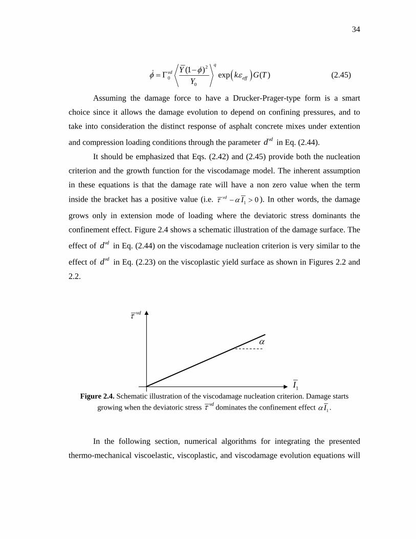
34
2
00
(1 )exp ( )
q
vdeff
Yk G T
Y
(2.45)
Assuming the damage force to have a Drucker-Prager-type form is a smart
choice since it allows the damage evolution to depend on confining pressures, and to
take into consideration the distinct response of asphalt concrete mixes under extention
and compression loading conditions through the parameter vdd in Eq. (2.44).
It should be emphasized that Eqs. (2.42) and (2.45) provide both the nucleation
criterion and the growth function for the viscodamage model. The inherent assumption
in these equations is that the damage rate will have a non zero value when the term
inside the bracket has a positive value (i.e. 1 0vd I ). In other words, the damage
grows only in extension mode of loading where the deviatoric stress dominants the
confinement effect. Figure 2.4 shows a schematic illustration of the damage surface. The
effect of vdd in Eq. (2.44) on the viscodamage nucleation criterion is very similar to the
effect of vdd in Eq. (2.23) on the viscoplastic yield surface as shown in Figures 2.2 and
2.2.
Figure 2.4. Schematic illustration of the viscodamage nucleation criterion. Damage starts
growing when the deviatoric stress vd dominates the confinement effect 1I .
In the following section, numerical algorithms for integrating the presented
thermo-mechanical viscoelastic, viscoplastic, and viscodamage evolution equations will
vd
1I

35
be detailed, and the associated material constants will be indentified based on available
experimental data.
2.7. Numerical Implementation
As mentioned in the previous sections, the constitutive models are presented in the
effective (undamaged) configuration. This approach substantially simplifies the
numerical implementation since it avoids the complexities associated with the direct
couplings of the damage model to the viscoelastic and viscoplastic models. In other
words, one can first update the stress tensor in the effective configuration using the
viscoelastic and viscoplastic models, then calculate the damage variable which is
functions of the stress in the effective configuration, and finally update the nominal
strain and stress tensors. The strain increment in the nominal configuration is known
tij
at the beginning the analysis. For the strain equivalence hypothesis, the strain
increments in the effective and nominal configurations are the same. However, this is not
the case for other transformation hypotheses such as strain energy equivalence
hypothesis or power equivalence hypothesis. For these hypotheses, another iteration
scheme should be added to the numerical implementation in order to obtain the
converged strain increment in the effective configuration. Having the given strain
increment, t t tij ij ij , and values of the stress and internal variables from the
previous step (i.e. at time t t ), one can obtain the updated values at the end the time
increment (i.e. at time t). Therefore, one can decompose the total strain in Eq. (2.1), the
effective viscoplastic strain in Eq. (2.26), and the effective stress tensor ij ,
respectively, at the current time t as follows:
, , , , , ,t nve t vp t t t t nve t t vp t t nve t vp tij ij ij ij ij ij ij ij ij (2.46)
t t t tp p p (2.47)
t t t tij ij ij (2.48)

36
In the next subsections, the procedure for determination of ,ve tij , ,vp t
ij , tp ,
and tij will be explained. Moreover, in the following subsections, the constitutive
model is assumed to be at the reference temperature (i.e. 0T T ), such that all
temperature coupling terms have the value of one. In this section, a step by step
procedure for implementation of the proposed complex constitutive model is presented.
In other words, at the beginning, the procedure for implementation of the viscoelastic
model is explained, then the viscoelastic model is coupled to viscoplasticity, and finally
the coupled viscoelastic-viscoplastic model will be coupled to the damage models.
2.7.1. Implementation of the Viscoelastic Model
Deviatoric and volumetric components of the viscoelastic strain tensor can be rewritten
as follows by using (2.16) and (2.17) (Haj-Ali and Muliana, 2004):
, , ,
1 1 ,1
2 1 11
1exp( )
2
1 exp( ) 1 exp( )1
2
nve t nve t nve t tij ij ij
Nt t tt t t t t t t t tij ij n n ij n
n
t t tNt t t t t t tn n
n ijt t tn n n
e e e
J S J S J g t g q
t tg J g g S
t t
(2.49)
, , ,
1 1 ,1
2 1 11
1exp( )
3
1 exp( ) 1 exp( )1
3
nve t nve t nve t tkk kk kk
Nt t tt t t t t t t t tkk kk n n kk n
n
t t tNt t t t t t tn n
n kkt t tn n n
B B B g t g q
t tg B g g
t t
(2.50)
where the variables ttnijq
, and ttnkkq
, are the deviatoric and volumetric components of the
hereditary integrals for each term n of the Prony series at previous time step tt ,
respectively. The hereditary integrals are updated at the end of each converged time
increment, which will be used for the next time increment, and are expressed as follows
(Haj-Ali and Muliana, 2004):
, , 2 2
1 exp( )exp( ) ( )
tt t t t t t t t t t nij n n ij n ij ij t
n
q q g S g S
(2.51)

37
, , 2 2
1 exp( )exp( ) ( )
tt t t t t t t t t t nkk n n kk n kk kk t
n
q q g g
(2.52)
The problem in solving Eqs. (2.49) and (2.50) is that the nonlinear functions are
not known at the current increment t . Therefore, an iterative method can be used to find
the correct stress state. Hence, Eqs. (2.49) and (2.50) are further linearized by assuming
that t t tg g , such that the trial stress increment can be written as follows:
, ,1 ,,
1
1 1exp( ) 1
2
Nt tr t t tr t t
ij ij n n ij nt trn
S e g J t qJ
(2.53)
, ,1 ,,
1
1 1exp( ) 1
3
Nt tr t t tr t tkk kk n n kk nt tr
n
g B t qB
(2.54)
where ,t trJ and ,t trB can be obtained using Eqs. (2.16) and (2.17) when the nonlinear
parameters are functions of the trial stress. This study employs the iterative scheme to
obtain the correct stress for a given strain increment. Before the onset of viscoplasticity,
the residual strain will be defined as follows:
, , ,1
3ve t ve t ve t tij ij kk ijR e (2.55)
The Newton-Raphson method will be used to minimize the strain residual in Eq. (2.55).
Moreover, when the strain is totally viscoelastic, the program uses the consistent
Jacobian matrix which is the consistent tangent compliance and is determined as:
,
1, 2
1ˆ ˆ ˆ3
ˆ ˆ ˆ1
3
1 exp( )1 ˆ exp( )2
ve tijve t t t
ijkl ik jl ij kltij
t t t teff t t
ij kk ijt t t tkl eff eff eff
ttt t t t t t tn
n n ij n ijt teff n
RS J B J
J B J
tgJ t q g S
t
1
1, 2
1
1 exp( )1 ˆ exp( )9
N
n
tt Nt t t t t t tn
n n kk n kk ijt tneff n
tgB t q g
t
(2.56)
It should be noted that Eqs. (2.55) and (2.56) are not valid in the presence of the
viscoplastic strains. These equations will be updated in the next subsection. Figure 2.5

38
shows the flowchart for implementation of the viscoelastic model. Note that, this
flowchart is valid in the absence of viscoplasticity and damage. Hence, the nominal
strain increment will be the same as the strain increment in the healed configuration.
Figure 2.5. The flow chart of the recursive-iterative algorithm for implementation of the viscoelastic model.
2.7.2. Implementation of the Viscoplastic Model
The viscoplastic strain increment in Eqs. (2.19) and (2.20) can be rewritten as follows:
Known , , g , ,ij nq at time t t
Assume ,tr t t tg g and calculate trial stress ,tr t
ijS [Eq. (2.53)] and ,tr tkk [Eq. (2.54)]
Correct trial stress Eqs. (2.53) and (2.54).
,ve tijR Tolerance
Update , g , ,ij nq , and ,kk nq at time t
No
Yes
Given t which is equal to t .
Recalculate tg based on the current trial stress.
Calculate the consistent tangent compliance veijklS [Eq.(2.56)] and stress
correction.
Calculate the residual strain veijR [Eq. (2.55)].

39
, ,N
vp t vp vp tij
ij ij
F Ff t
(2.57)
where ,vp t can be written from Eqs. (2.20) and (2.21) as follows:
,
,0
,N
t vp tN ij evp t vp vp
y
ft f t
(2.58)
Substituting Eqs. (2.26), and (2.57) into Eq. (2.47), the effective viscoplastic
strain increment can be written as:
,
, , , ,vp t
vp t vp t t vp t vp t te e e e
ij ij
F F
a
(2.59)
According to Wang et al. (1997), one can define a consistency condition for rate-
dependent plasticity (viscoplasticity) similar to the classical rate-independent plasticity
theory such that a dynamic (rate-dependent) yield surface, , can be expressed from
Eqs. (2.20), (2.21), and (2.22) as follows:
1/
01 0
Nvpvp
y vpI p
(2.60)
The Kuhn-Tucker loading-unloading condition (consistency) is valid also for the
dynamic yield surface , such that:
0; 0; 0; 0vp vp (2.61)
A trial dynamic yield surface function tr can be defined using Eqs. (2.53), (2.54), and
(2.60), such that:
1/,
, 01
Nvp t ttr vp tr tr t t
y vpI p
t
(2.62)
,vp t and tp can be obtained by iteratively solving Eq. (2.62) using the Newton-
Raphson scheme. Once ,vp t is obtained, the viscoplastic strain increment vpij can
then be obtained from Eq. (2.57). In the Newton-Raphson scheme, the differential of
with respect to vp is needed, which can be expressed as follows:

40
10 vp Ny
vp vp vp vp
p
p N t
(2.63)
At the k+1 iteration, the viscoplastic multiplier can be calculated as follows:
1
1, ,,
kk kvp t vp t k
vp t
(2.64)
The above recursive-iterative algorithm with the Newton-Raphson method is used to
obtain the current effective stress and the updated values of viscoelastic and viscoplastic
strain increments by minimizing the residual strain defined as:
, ,nve t vp t tij ij ij ijR (2.65)
The stress increment at the k+1 iteration is calculated by:
1
1kt
k k kijt t tij ij klt
kl
RR
(2.66)
where the differential of tijR gives the consistent tangent compliance, which is necessary
for speeding convergence and can be derived as follows:
, ,
, ,t nve t vp tij ij ij nve t vp t
ijkl ijkl ijklkl kl kl
RS S S
(2.67)
where ,
,nve t
ijnve tijkl
kl
S
is the nonlinear viscoelastic tangent compliance which is derived
in Eq. (2.56). The viscoplastic tangent compliance can be derived using Eqs. (2.22),
(2.57), and (2.58), such that:
, , 2, ,
12
0 0 0
vp t vp tijvp t vp t
ijklkl ij kl ij kl
N Nvp
vp
y y ij kl y ij kl
F FS
t N f F f f Ft
(2.68)

41
The tangent compliance for the coupled viscoelastic-viscoplastic model can now be
obtained by substituting Eqs. (2.56) and (2.68) into Eq. (2.67). The flowchart for
implementing the coupled viscoelastic-viscoplastic model is presented in Figure 2.6.
2.7.3. Implementation of the Viscodamage Model
Damage is implemented using the effective configuration concept. Using the effective
configuration concept substantially simplifies the numerical implementation of the
damage model and avoids the complexities associated with the direct couplings of the
viscoelastic and viscoplastic models to the damage model.
In other words, the stress in the effective configuration can be first updated using
the viscoelastic and viscoplastic models. The damage force which is expressed in terms
of the quantities in the effective configuration can be calculated and used to calculate the
damage rate. The damage dynamic surface can be obtained using Eq. (2.45), such that:
0
1exp 0vd
eff vd
qY
kY
(2.69)
where Y is the damage force and vd is the damage loading condition. A trial value for
viscodamage loading surface can be defined as:
,
0
1exp 0
t t t tvd tr
eff vd
qY
kY t
(2.70)
Very similar to viscoplasticity, the damage increment can be obtained using the Newton-
Raphson scheme. However, it should be noted that the values of Y and eff are constant
during these trials, which substantially simplifies the implementation, since they are
expressed in the healed configuration. However, the differential of the vd with respect
to is needed which can be expressed as follows:
0 0
11 1
expvd
eff vd
qYY
kY Y t
(2.71)

42
Figure 2.6. The flow chart of the recursive-iterative Newoton-Raphson algorithm for implementation of the coupled viscoelastic-viscoplastic model.
Calculate the residual strain ijR [Eq.
(2.65)].
Calculate veije and ve
kk from Eqs. (2.49) and (2.50).
Put , 0vp tij .
Calculate vpij and p based on the current
trial stress by using the local Newton-Raphson method [Eq. (2.64)].
Correct trial stress [Eq.(2.66)].
tijR Tolerance
No Yes
No No
Yes Yes
Known , ve , vp , g , ,ij nq , p , vp at time t t
Given t which is equal to t .
Calculate trial stress ,tr tijS [Eq. (2.53)] and ,tr t
kk [Eq. (2.54)].
Recalculate tg based on the current trial stress.
Calculate the consistent tangent compliance ijklS [Eq. (2.67)] and stress
correction [Eq. (2.66)].
Update , ve , vp , g , ,ij nq , p at time t
1 0vpf I

43
Hence, the damage density increment at the 1k iteration can be obtained as follows:
1
1kvd
k kt t vdt
(2.72)
The damage density can then be obtained, such that:
t t t t t (2.73)
Finally, Eq. (2.6) can be used to update the final nominal stress. It should be noted that
the healing process is not included in this damage model. Hence, negative damage
density rates are not accepted and are set to zero.
The above formulated numerical algorithms are implemented in the well-known
commercial finite element code Abaqus (2008) via the user material subroutine UMAT.
The finite element model considered here is simply a three-dimensional single element
(C3D8R) available in Abaqus.
This subsection concludes the numerical implementation of the proposed
viscoelastic-viscoplastic-viscodamage-healing model.
2.8. Application of the Model to Asphalt Concrete: Model Calibration
In this section, the presented thermo-viscoelastic-viscoplastic-viscodamage constitutive
model is calibrated using a set of experimental data on asphalt concrete tested at
different stress levels, strain rates, and temperatures. The asphalt concrete used in this
study is described as 10 mm Dense Bitumen Macadam (DBM) which is a continuously
graded mixture with asphalt binder content of 5.5%. Granite aggregates and an asphalt
binder with a penetration grade of 70/100 are used in preparing the asphalt mixtures.
Cylindrical specimens with a diameter of 100mm and a height of 100mm are compacted
using the gyratory compactor. Single creep-recovery test under direct compression at the
reference temperature is conducted to identify the viscoelastic and viscoplastic model
parameters, whereas, two creep tests that include the tertiary creep response at the
reference temperature are conducted to identify the viscodamage model parameters. The
healing model parameters are also identified using the repeated creep-recovery test with

44
rest period at the reference temperature. The temperature coupling term parameters are
then identified by comparing the results at different temperatures. Moreover, the
parameters that distinguish between compressive and extensive loading conditions (i.e.
vpd and vdd ) are identified by comparing several tests in tension and compression.
Finally, the identified model parameters are used to predict the mechanical
response of asphalt concrete over an extensive experimental data including creep-
recovery, creep, constant strain rate test, and repeated creep-recovery tests over a range
of temperatures, stress levels, loading-unloading times, and strain rates in both tension
and compression. Table 2.1 lists the summary of the tests used for calibration of the
model.
The procedure for identification of the viscoelastic, viscoplastic, and
viscodamage model parameters is presented by Darabi et al. (2011c). The procedure for
identification of the model parameters will be explained in the next sub-sections.
Table 2.1. The summary of the tests used to identify the model parameters.
Test Temperature ( o C ) Stress level (kPa) Loading time (Sec)
Compression
Creep-recovery 20 1500 30
Creep 10 2000 20 1000, 1500 40 500
Tension Creep 20 300, 500
2.8.1. Identification of the Viscoelastic Model Parameters
The first step in calibration process is to determine the viscoelastic model parameters at
the reference temperature. To achieve this, the viscoelastic and viscoplastic responses in
the recovery part of a single creep-recovery test should be separated. The advantage of
conducting a creep-recovery test is that the viscoplastic strain during the recovery
remains constant which makes it possible to separation the viscoelastic and viscoplastic
strains. Figure 2.7 (a) shows a schematic single creep-recovery test in which the stress

45
level is kept constant up to time at and is removed after time at . The strain response
of the creep-recovery loading [Figure 2.7 (a)] is presented in Figure 2.7 (b).
It should be noted that the stress level in the conducted creep-recovery test
should be low and/or the loading time should be short such that the material does not get
damaged or at least the induced damage can be assumed to be negligible. The strain
response at the end of the loading time at can be decomposed into viscoelastic and
viscoplastic components, such that:
ve vpa a at t t (2.74)
Figure 2.7. A schematic creep-recovery test.
The same strain decomposition can be assumed for any time t after the unloading
time at (i.e. at t ). However, the stress is zero during the recovery. Hence, the
viscoplastic strain remains constant after the unloading time at (i.e.
t
at
at
att
at t
Time
Time
Stress
Strain
(a)
(b)

46
vp vpa at t t ). Hence, one can write the following strain decomposition at point
at t :
ve vpa at t t t (2.75)
Subtracting Eq. (2.75) from Eq. (2.74) and calculating veat and ve t using
Eqs. (2.7) and (2.9) yield:
1 0 0 1 2ve ve
a a at t g D g g D t D t D t t (2.76)
A low stress level is applied in this creep-recovery test and , hence, the nonlinear
viscoelastic parameters can be assumed to be one (i.e. 0 1 2 1g g g ). Therefore, Eq.
(2.76) can be simplified as follows for low stress levels:
1 0ve ve
a a at t D D t D t D t t (2.77)
1ve can be calculated for each test data in the recovery region. Note that the right hand
side of Eq. (2.77) is only a function of viscoelastic properties. Therefore, the linear
viscoelastic model parameters nD and n (i.e. the Prony series coefficients, Eq. (2.9))
can be identified by minimizing the error between the experimental measurements for
1ve and Eq. (2.77).
2.8.2. Identification of the Viscoplastic Model Parameters
The next step in the model calibration process is to identify the viscoplastic model
parameters. Basically, the creep part of the analyzed creep-recovery test [Figure 2.7] can
be used to identify the viscoplastic model parameters at the reference temperature. In
other words, the viscoplastic strain in the creep part can be obtained by subtracting the
model prediction for the viscoelastic strain (using the viscoelastic model parameters
obtained in the previous sub-section) from the total experimental measurements.
The dynamic viscoplastic yield surface in Eq. (2.60) for a uniaxial compression
step-loading is expressed as:
1
0 1 2 01 exp 03
vp Ny
vpp
(2.78)

47
where is the applied uniaxial compressive stress. Rearranging Eq. (2.78) yields:
0 1 2
0
1 exp3
N
vpvp
y
p
t
(2.79)
where vp can be obtained using the separated viscoplastic strain in the creep region
,1vp t using the following expression [Eq. (2.57)]:
,
1
13
vp tvp
(2.80)
Moreover, the effective viscoplastic strain for the uniaxial compression can be calculated
using Eq. (2.59) as follows:
2 2
1 2
12vp vpp
a (2.81)
where 2
0.5 31 2
1 3a
. 1vp and 2
vp are the axial and radial viscoplastic
strain increments, respectively. However, the available experimental data does not
include 2vp . Hence, one can calculate 2
vp using Eq. (2.19), such that:
,
2,
1 22 11
1.5/
3
vp t
vp t
F F
(2.82)
Once p is calculated from the analyzed experimental data using Eqs. (2.80) and (2.81),
the viscoplastic model parameters vp , N , 0 , 1 , and 2 can be identified by
minimizing the error between the measurements and Eqs. (2.79) and (2.81).
Figure 2.8 shows the separation of the viscoelastic and viscoplastic strains at the
reference temperature (i.e. 20oT C ) when the applied stress is 1500 kPa and the
loading time is 30 sec. As mentioned before, the shortest loading time is selected to
identify the viscoelastic and viscoplastic model parameters such that one can reasonably
assume that the induced damage is negligible at these loading conditions. The
viscoelastic and viscoplastic model parameters can now be identified by fitting the

48
separated viscoelastic and viscoplastic strains as shown in Figure 2.8(b). Finally, the
model predictions and experimental measurements for the total strain at the reference
temperature are presented in Figure 2.8(c).
(a)
(b)
Figure 2.8. Identification of the viscoelastic and viscoplastic model parameters using a creep-recovery test at the reference temperature (i.e. 20oT C ) when the applied stress is 1500kPa
and the loading time is 30 sec. (a) Separation of the viscoelastic and viscoplastic strains using the experimental data; (b) Experimental and model predictions for the viscoelastic strain and the
viscoplastic strain; (c) Experimental and model prediction of the total strain.
0.0
0.2
0.4
0.6
0.8
1.0
1.2
0 100 200 300 400 500
Stra
in (%
)
Time (Sec)
Experimental data for total strain
Separated viscoelastic strain
Separated viscoplastic strain
0.0
0.1
0.2
0.3
0.4
0.5
0.6
0 100 200 300 400 500
Stra
in (%
)
Time (Sec)
Separated viscoelastic strain, Experimental data
Model prediction of viscoelastic strain
Separated viscoplastic strain, Experimentl data
Model prediction of viscoplastic strain

49
(c)
Figure 2.8. Continued.
2.8.3. Identification of the Viscodamage Model Parameters
The loading times in the creep-recovery tests conducted to identify the viscoelastic and
viscoplastic model parameters are too short for the material to get damaged. However, in
other tests such as the creep tests, the load usually remains on the specimen until failure.
The loading time in these tests are long enough for damage to evolve causing the
secondary and tertiary creep responses. The damage model is calibrated using the
secondary and tertiary creep responses in a creep test since these regions are mostly
caused by damage. Moreover, during the creep loading, healing does not occur in the
material which makes it possible to calibrate the damage model independent of the
healing effects. To calibrate the viscodamage model at the reference temperature (i.e.
20oT C ), the identified viscoelastic and viscoplastic model parameters at the reference
temperature are used to predict the creep tests. These predictions usually match for the
initial response and start deviating from the experimental measurements in secondary
and tertiary creep regions. This deviation should be compensated for by using the
viscodamage model.
0.0
0.2
0.4
0.6
0.8
1.0
1.2
0 100 200 300 400 500
Tota
l str
ain
(%)
Time (Sec)
Experimental data
Model prediction

50
At the reference temperature, the viscodamage temperature coupling term has the
value of one [i.e. 0 1G T ]. Therefore, at the reference temperature, Eq. (2.45)
simplifies as follows:
2
00
(1 )exp
q
vdeff
Yk
Y
(2.83)
The first step in identifying the viscodamage model parameters is to select an
arbitrary reference stress level (which is selected to be 1000kPa in this work). The
reference damage force 0Y can be calculated easily using Eq. (2.42) as the reference
damage force. The damage evolution law of Eq. (2.83) can be expressed in terms of the
damage force in the nominal configuration by making use of Eq. (2.43), such that:
00
exp( )q
vdeff
Yk
Y
(2.84)
However, the nominal stress during the creep test is constant. Hence, at the reference
stress level, the damage force Y is the damage force at the reference stress level.
Therefore, at the reference stress level, Eq. (2.84) can be simplified further as:
0 exp( )vdeffk (2.85)
Now, the damage viscosity parameter vd and the strain dependency parameter k can be
identified using a creep test at the reference temperature and stress level. The
viscodamage stress dependency parameter q can finally be identified by comparing the
experimental results and model predictions for a creep at another stress level (i.e.
1500kPa in this work) which is different from the reference stress level.
The identified model viscoelastic-viscoplastic-viscodamage model parameters at
the reference temperature are listed in Table 2.2.
Figure 2.9 shows the comparison between the model prediction and the
experimental data for those creep tests that have been used to identify the viscodamage
model parameters. Figure 2.9 clearly shows that the model is capable of capturing both
secondary and tertiary behavior in the creep test.

51
Table 2.2. The identified viscoelastic-viscoplastic-viscodamage model parameters at the reference temperature.
Viscoelastic model parameters n 1 2 3 4 5
n (sec-1) 10 1 0.1 0.01 0.001
nD (kPa-1) 1.98 10-7 1.48 10-6 6.56 10-7 1.43 10-6 2.74 10-6
0D (kPa-1) 3.5 10-6
Viscoplastic model parameters vp (sec-1) N
0 (kPa) 1 (kPa) 2
0.3 0.15 5 10-4 3.63 35 610 215 Viscodamage model parameters
vd (sec-1) 0Y (kPa) q k
4 10-5 700 5 30
Figure 2.9. Model predictions and experimental measuremenst for the creep test at the reference temperature (i.e. 20oT C ) and two different stress levels. These two test are used to identify
the viscodamage model parameters.
2.8.4. Identification of the Model Parameters Distinguishing between Loading Modes
One of the main advantages of the model is the presence of two parameters vpd and vdd
that enables the model to distinguish between the compressive or extension mode of
loadings. vpd is a material parameter representing the sensitivity of yield behavior to the
0
1
2
3
4
5
6
7
8
9
10
0 500 1000 1500 2000 2500 3000
Axi
al c
reep
str
ain
(%)
Time(Sec)
Experimental data, stress=1500 kPa
Model prediction,stress= 1500 kPa
Experimental data, stress= 1000 kPa
Model prediction, stress=1000 kPa

52
hydrostatic pressure 1I . This parameter can also be defined as the ratio of the yield
strength in uniaxial tension to that in uniaxial compression (i.e. t c/vpy yd ). Similarly,
vdd captures the different damage responses in extension and compression. In fact, vdd
magnifies the damage force Y in tensile loading modes. These two parameters can be
obtained by comparing experimental measurements and model predictions in tension and
compression. In this study, 0.78vpd and 0.16vpd are identified. Figure 2.10 shows
the model prediction and experimental measurements of the creep test at 20oC when the
applied tensile stresses are 300kPa and 500kPa. Figure 2.10 clearly shows that using vpd
and vdd parameters enhance the model predictions through distinguishing the behaviors
in tension and compression.
Figure 2.10. Model predictions and experimental measuremenst for the creep test in tension at
20oC and different stress levels. These tests are utilized to identify vpd and vdd model parameters.
2.8.5. Identification of the Temperature Coupling Term Model Parameters
It is not convenient to introduce a whole different set of material parameters for each
temperature as done by Abu Al-Rub et al. (2009) and Huange et al. (2011a). Therefore,
0.0
0.5
1.0
1.5
2.0
2.5
0 100 200 300 400 500
Axi
al st
rain
(%
)
Time (Sec)
Experimental data
Model prediction
500 kPa
300 kPa

53
in this study, the model’s ability to predict the response at other temperatures is achieved
through the temperature coupling terms as discussed next.
The viscoelastic-viscoplastic material responses at other temperatures can be
captured using the temperature time-shift factor for both viscoelasticity and
viscoplasticity. The reduced time concept [Eq. (2.8)] can be used for introducing the
temperature time-shift factor veTa in the viscoelasticity constitutive equations; whereas,
the viscoplasticity constitutive equations are coupled to temperature by replacing the
time increment t with the reduced time increment / vpTt a , such that the dynamic
viscoplasticity yield surface in Eq. (2.60) can be rewritten as follows:
1/
01 0
N
vpvp
yvp
vpT
I pt
a
(2.86)
where vpTa is the viscoplasticity temperature coupling term or the viscoplasticity
temperature time-shift factor. Note that Eq. (2.86) implies that the viscoplasticity
temperature coupling term should also be introduced in the viscoplasticity flow rule, Eq.
(2.19), such that:
,N
vp t vpij vp
ijT
t Ff
a
(2.87)
In this study, the same temperature coupling terms are assumed for both the
viscoelastic and viscoplastic models (i.e. ve vpT T Ta a a ) as suggested by the
experimental study of Schwartz et al. (2002) on asphalt mixtures. The values of the
viscoelastic and viscoplastic temperature coupling parameters are obtained from the
creep-recovery tests at different temperatures. The creep compliance ( )D t can be
calculated using experimental data at different temperatures [see Figure 2.10] using the
following relation:
( )
( )t
D t
(2.88)

54
Figures 2.11 (a) and (b) show the experimental data at different temperatures before and
after shifting, respectively. By shifting the experimental data horizontally, one can get
the viscoelastic-viscoplastic temperature time-shift factor, Ta , for each temperature.
(a)
(b)
Figure 2.11. Experimental data for creep compliance at 10T , 20, and 40oC . (a) Before applying the temperature time-shift factor. (b) After applying the temperature time-shift factor.
0
2
4
6
8
10
12
14
16
0 1 2 3 4 5 6 7
Ln(
D(t
)), [
kPa-
1]
Ln (t) (sec)
Temp=10
Temp=20
Temp=40
0
2
4
6
8
10
12
14
16
-2 0 2 4 6 8 10 12
Ln
(D(t
)),
[kP
a-1]
Ln( t/aT)
Temp=10
Temp=20
Temp=40

55
The reduced time (or time-shift) concept as used in viscoelasticity and
viscoplasticity for including temperature effects can also be used in the viscodamage
model for predicting the damage evolution in asphalt mixes at different temperatures.
Similarly, one can replace the time increment t in the damage evolution
equation [Eq. (2.45)] with the reduced time / vdTt a , such that Eq. (2.45) can be
rewritten as:
00
expq
vdeff vd
T
Y tk
Y a
(2.89)
where 1vd
TaG T
is the viscodamage temperature time-shift factor. In this study, two
creep tests at temperatures 10oC and 40oC are used to determine the temperature
coupling terms. Figure 2.12 represents the model predictions and experimental
measurements for the creep test at 10oC and 40oC. These two tests are used in order to
identify the temperature coupling term model parameters.
Figure 2.12. Model predictions and experimental measuremenst for the creep test at different
temperatures in order to identify the temperature coupling term parameters for the viscodamage model.
0
1
2
3
4
5
6
7
8
9
10
0 500 1000 1500 2000 2500 3000
Axi
al c
reep
str
ain
(%)
Time(Sec)
10 ; 2000kPaoT C
40 ; 500kPaoT C
Experimental data
Model prediction

56
Arrhenius-type equations are used for expressing the viscoelastic, viscoplastic,
and viscodamage temperature coupling terms, such that one can write:
10
exp 1vpT T
Ta a
T
(2.90)
20
exp 1vdT
Ta
T
(2.91)
where 1 and 2 are material parameters and 0T is the reference temperature. . The
identified temperature coupling term parameters are listed in Table 2.3.
Table 2.3. Temperature coupling term model parameters [Eqs. (2.90) and (2.91)].
1 2
-4.64 -5.89
It is noteworthy that assuming the same temperature time-shift factor for both
viscoelasticity and viscoplasticity saves significant amount of experimental tests needed
for calibrating the thermo-viscoplastic response of asphaltic materials. Figure 2.13
shows the flowchart for obtaining the model parameters in a systematic manner.

57
Figure 2.13. The procedure for identification of the thermo-viscoelastic-viscoplastic-viscodamage constitutive model parameters.
2.9. Application of the Model to Asphalt Concrete: Model Validation
The identified model parameters listed in Tables 2.2 and 2.3 are used to validate the
model against another set of experimental data listed in Table 2.4 which have not been
used in the calibration process. Table 2.4 shows that the model is to be validated against
different sets of experimental data including creep-recovery, creep, repeated creep-
recovery, and uniaxial constant strain rate tests in both tension and compression at
different temperatures, stress levels, and strain rates.
Separate viscoelastic response in the recovery part of the creep-recovery tests using Eq. (2.76).
Identify the Prony series coefficients nD and n at the reference temperature using
Eqs. (2.9) and (2.76).
Calculate 1vp , 2
vp , and p from the creep part of the creep-recovery tests using Eqs.
(2.80), (2.81), and (2.82).
Identify the viscoplastic model parameters at the reference temperature by minimizing the error between the experimental measurements and Eq. (2.79).
Identify vd and k from a creep test at the reference temperature and stress level using Eq. (2.85).
Identify viscodamage stress dependency parameter q from a creep test at the
reference temperature, when ref using Eq. (2.84).
Identify temperature coupling terms model parameters by comparing experimental data and model predictions at different temperatures using Eqs. (2.90) and (2.91).
Identify vpd and vpd from two creep tests in tension using Eqs. (2.23) and. (2.44).

58
Table 2.4. The summary of the tests used for validating the model.
Test Temperature
( o C ) Stress level
(kPa) Loading time
(Sec) Strain rate
(Sec-1) C
omp
ress
ion
Creep-recovery
10 2000 400, 600 2500 350, 300
20 1000 40, 210 1500 130
40 500 130, 180 750 35
Creep 10 2500 40 750
Constant strain rate
10 0.005, 0.0005,
0.00005
20 0.005, 0.0005,
0.00005 40 0.005, 0.0005
Repeated creep-recovery
20 1500 120 (100)*, 60 (100),
60 (1500)
Ten
sion
Creep 10 500, 1000, 1500 20 700 35 100, 150
Constant strain rate
20 0.0167, 0.00167
Repeated creep-recovery
20 300 120 (100), 60 (50), 60 (100), 60 (1500)
*Unloading time in second.
2.9.1. Model Validation against Creep-Recovery Tests
Creep-recovery tests at 10, 20, and 40oC for different stress levels and loading times are
conducted in this section in order to validate the model. Model predictions and
experimental measurements for the creep-recovery test in compression at temperatures
10, 20 , and 40o C are shown in Figures 2.14, 2.15, and 2.16, respectively. Figures 2.14
and 2.15 show that at temperatures 10o C and 20o C the model can reasonably predict
the experimental data at different stress levels and loading times. Figure 2.16 shows that
the model underestimates the experimental measurements at temperature 40o C at tress
level 500 kPa. Although Figure 2.16 shows that the model yields reasonable predictions
at stress level 750 kPa, more experimental measurements at high temperatures are still
needed to more accurately identify the viscoelastic-viscoplastic temperature coupling
terms.

59
(a)
(b)
Figure 2.14. Experimental measurements and model predictions for creep-recovery test in compression at 10oT C ; (a) 2000 kPa, (b) 2500 kPa.
0.0
0.5
1.0
1.5
2.0
2.5
3.0
0 500 1000 1500 2000 2500 3000
Tota
l str
ain
(%)
Time (Sec)
Experimental data, LT=600 Sec
Model prediction, LT=600 Sec
Experimental data, LT=400 Sec
Model prediction, LT=400 Sec
0.0
0.5
1.0
1.5
2.0
2.5
3.0
0 500 1000 1500 2000 2500 3000
Tota
l str
ain
(%)
Time (Sec)
Experimental data, LT=350 Sec
Model prediction, LT=350 Sec
Experimental data, LT=300 Sec
Model prediction, LT=300 Sec

60
(a)
(b)
Figure 2.15. Experimental measurements and model predictions for creep-recovery test in compression at 20oT C ; (a) 1000 kPa, (b) 1500 kPa.
0.0
0.5
1.0
1.5
2.0
0 500 1000 1500 2000 2500 3000
Tota
l str
ain
(%)
Time (Sec)
Experimental data, LT=210 Sec
Model prediction, LT=210 Sec
Experimental data, LT=40 Sec
Model prediction, LT=40 Sec
0.0
0.5
1.0
1.5
2.0
2.5
0 500 1000 1500 2000 2500 3000
Tota
l str
ain
(%)
Time (Sec)
Experimental data, LT=130 Sec
Model prediction, LT=130 Sec

61
Figure 2.16. Experimental measurements and model predictions for creep-recovery test in compression at 40oT C .
2.9.2. Model Validation against Creep Tests
Figure 2.17 shows the model predictions and experimental measurements for creep test
in compression for different temperatures and stress levels. Figure 2.17 shows that the
model is able to capture the tertiary behavior very close to the experimental
measurements. It is noteworthy that the failure time changes drastically from thousands
of seconds to couple of hundred seconds as the stress level changes. Figure 2.17(b)
shows that even at temperature 40o C the model can capture secondary and tertiary
creep reasonably.
The model is further validated by comparing the model predictions and
experimental measurements for the creep tests in tension at different temperatures and
stress levels. Model predictions and experimental measurements for the creep-test in
tension for a range of temperatures and stress levels are compared in Figure 2.18.
500kPa;LT=180sec
Experimental data
Model prediction0.0
0.5
1.0
1.5
2.0
2.5
3.0
0 100 200 300 400 500
Tota
l str
ain
(%)
Time (Sec)
750kPa;LT=35sec

62
(a)
(b)
Figure 2.17. Experimental measurements and model predictions for the creep test in
compression at different temperatures and stress levels. (a) 10 ; 2500kPaoT C ; (b)
40 ; 750kPaoT C .
0
1
2
3
4
5
6
7
8
9
10
0 10 20 30 40 50 60 70 80
Axi
al c
reep
str
ain
(%)
Time(Sec)
Experimental data
Model prediction
o750 kPa;T=40 C
0
1
2
3
4
5
6
7
8
9
10
0 500 1000 1500 2000
Axi
al c
reep
str
ain
(%)
Time(Sec)
Experimental data
Model prediction
o2500 kPa;T=10 C

63
Figure 2.18. Experimental measurements and model predictions for creep test in tension. (a)
10oT C ; (b) 20oT C ; (c) 35oT C .
0.0
0.5
1.0
1.5
2.0
2.5
0 50 100 150 200
Axi
al st
rain
(%
)
Time (Sec)
Experimental data
Model prediction
150 kPa
100 kPa(c)
0.0
0.5
1.0
1.5
2.0
2.5
0 5 10 15 20 25 30 35 40
Axi
al st
rain
(%
)
Time (Sec)
Experimental data
Model prediction
700 kPa(b)
0.0
0.5
1.0
1.5
2.0
2.5
0 300 600 900 1200 1500
Axi
al st
rain
(%
)
Time (Sec)
Experimental data
Model prediction
1500 kPa
1000 kPa
500 kPa
(a)

64
Figure 2.18 shows that the model is also capable of predicting the tertiary
behavior in tension. This figure shows that at temperatures 10 and 20o C the model can
predict the experiments well. Although model predictions and experimental
measurements are not quite the same at temperature 35o C , the model can still predict
the tertiary behavior rather reasonably. It should be mentioned that the distinction
between compression and tension is brought to the model through vpd and vdd
parameters.
2.9.3. Model Validation against Uniaxial Constant Strain Rate Tests
Different predictions are conducted in this chapter to validate the model in capturing the
time-, temperature-, and rate-dependent properties of bituminous materials. Therefore,
the model is also validated against the monotonic uniaxial constant strain rate tests in
compression at different temperatures in order to test the model capability in capturing
the temperature-dependent response of bituminous materials. Figure 2.19 shows the
stress-strain plots at different temperatures when the strain rate is 0.005/sec. Figure 2.19
clearly shows that the model is able to capture the temperature effects on the initial, peak
point, and post peak responses in the stress-strain diagram using the identified model
parameters presented in Tables 2.2 and 2.3. The plots of the predicted damage density
versus the total strain for strain rate of 0.005/sec is shown in Figure 2.19(b). Figure
2.19(b) shows that the damage density is close to zero at low strain levels and increases
as strain and stress levels increases. However, the rate of damage decreases after the
strain reaches close to 3%. This strain level corresponds to the strain at which the
maximum value of the stress occurs. This behavior is due to the presence of the damage
history term [i.e. 21 ] in the damage model in Eq. (2.45). In other words, the history
term causes the damage rate to decrease after the stress-strain peak point. Hence, one
may consider the inflection point of the damage-strain diagram as the strain corresponds
to the peak stress at the stress-strain diagram.
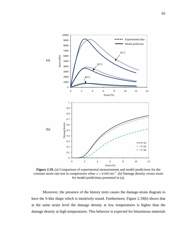
65
Figure 2.19. (a) Comparison of experimental measurements and model predictions for the
constant strain rate test in compression when 0.005 sec-1. (b) Damage density versus strain for model predictions presented in (a).
Moreover, the presence of the history term causes the damage-strain diagram to
have the S-like shape which is intuitively sound. Furthermore, Figure 2.19(b) shows that
at the same strain level the damage density at low temperatures is higher than the
damage density at high temperatures. This behavior is expected for bituminous materials
0
0.1
0.2
0.3
0.4
0.5
0.6
0.7
0.8
0.9
1
0 2 4 6 8 10 12
Dam
age
dens
ity
Strain (%)
T=10
T=20
T=40
0
1000
2000
3000
4000
5000
6000
7000
8000
9000
10000
0 2 4 6 8 10 12 14
Stre
ss (k
Pa)
Strain (%)
Experimental data
Model prediction
10o C
20o C
40o C
(a)
(b)

66
since they are more susceptible to damage at low temperatures. Moreover, the same test
(i.e. constant strain rate test is conducted at two other strain rates of 0.0005/sec, and
0.00005/sec to test the model capability in capturing the rate-dependent response of
bituminous materials. Figures 2.20(a) and 2.21(a) show that the model can reasonably
predict experimental data at different strain rates as well.
Figure 2.20. (a) Comparison of experimental measurements and model predictions for the
constant strain rate test in compression when 0.0005 sec-1. (b) Damage density versus strain for model predictions presented in (a).
0
0.1
0.2
0.3
0.4
0.5
0.6
0.7
0.8
0.9
1
0 2 4 6 8 10 12
Dam
age
dens
ity
Strain (%)
T=10
T=20
T=40
0
1000
2000
3000
4000
5000
6000
0 2 4 6 8 10 12 14
Stre
ss (k
Pa)
Strain (%)
Experimental data
Model prediction
10o C
20o C
40o C
(a)
(b)
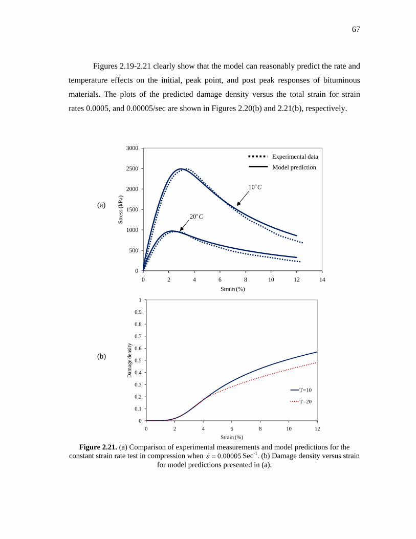
67
Figures 2.19-2.21 clearly show that the model can reasonably predict the rate and
temperature effects on the initial, peak point, and post peak responses of bituminous
materials. The plots of the predicted damage density versus the total strain for strain
rates 0.0005, and 0.00005/sec are shown in Figures 2.20(b) and 2.21(b), respectively.
Figure 2.21. (a) Comparison of experimental measurements and model predictions for the
constant strain rate test in compression when 0.00005 Sec-1. (b) Damage density versus strain for model predictions presented in (a).
0
0.1
0.2
0.3
0.4
0.5
0.6
0.7
0.8
0.9
1
0 2 4 6 8 10 12
Dam
age
dens
ity
Strain (%)
T=10
T=20
0
500
1000
1500
2000
2500
3000
0 2 4 6 8 10 12 14
Stre
ss (k
Pa)
Strain (%)
Experimental data
Model prediction
10o C
20o C
(a)
(b)
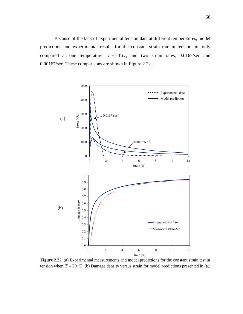
68
Because of the lack of experimental tension data at different temperatures, model
predictions and experimental results for the constant strain rate in tension are only
compared at one temperature, 20oT C , and two strain rates, 0.0167/sec and
0.00167/sec. These comparisons are shown in Figure 2.22.
Figure 2.22. (a) Experimental measurements and model predictions for the constant strain test in tension when 20oT C . (b) Damage density versus strain for model predictions presented in (a).
0
0.1
0.2
0.3
0.4
0.5
0.6
0.7
0.8
0.9
1
0 2 4 6 8 10 12
Dam
age
dens
ity
Strain (%)
Strain rate=0.0167/Sec
Strain rate=0.00167/Sec
0
1000
2000
3000
4000
5000
0 2 4 6 8 10 12
Stre
ss (k
Pa)
Strain (%)
Experimental data
Model prediction
-10.00167sec
-10.0167 sec(a)
(b)

69
Figure 2.22(a) shows that the model underestimates the experimental data at
strain rate of 0.0167/sec. However, reasonable predictions are obtained when at the
strain rate is 0.00167. Plots of the damage density versus the total strain for the
predictions presented in Figure 2.22(a) are shown in Figure 2.22(b). One can also see the
S-like shape of damage-strain diagram in Figure 2.22(b). However, since the peak stress
occurs very rapidly in tension, this S-like is not very clear, especially at higher strain
rates.
2.9.4. Model Validation against Repeated Creep-Recovery Tests
The ultimate goal of the current work is to develop a unified continuum model for
predicting the behavior of asphalt mixes during their service life. However, pavements
are subjected to repeated loading during the service life where fatigue damage becomes
very important. Thus, several repeated creep-recovery tests with different loading and
unloading times are utilized from the University of Nottingham database at the reference
temperature and compared with the model predictions. The applied stress level in
repeated creep-recovery tests in compression is 1500 kPa. Figure 2.23 shows the creep
strain-time diagram when the loading time is 120sec and the unloading time is 100sec.
As it is shown in Figure 2.23(a), the proposed model predictions compare well with the
experimental measurements. The damage evolution versus time is also presented in
Figure 2.23(b), which shows a stair case-type diagram for damage evolution which is
expected in repeated creep-recovery loading in case micro-damage healing (i.e. micro-
crack healing) is neglected. Figure 2.23 shows that during the loading period damage
evolves and during the unloading period the value of the damage density remains
constant in case the micro-damage healing is neglected.

70
(a)
(b)
Figure 2.23. (a) Comparison between model results and experiments for repeated creep-recovery test in compression when LT= 120 sec and UT=100 sec. (b) Damage density versus time.
However, several studies have shown that asphalt mixes experience healing
during the unloading duration (rest period) (Kim and Little, 1990; Lee and Kim, 1998;
Lee et al., 2000; Si et al., 2002; Little and Bhasin, 2007; Bhasin et al., 2008). In fact,
0.0
0.1
0.2
0.3
0.4
0.5
0.6
0.7
0.8
0.9
1.0
0 200 400 600 800
Dam
age
dens
ity
Time (Sec)
LT=120 Sec, UT=100 Sec
0
1
2
3
4
5
6
7
8
9
0 200 400 600 800 1000
Axi
al st
rain
(%
)
Time (Sec)
Experimental data
Model prediction
LT=120sec; UT=100sec

71
during the unloading process and resting time periods some micro-crack and micro-void
free surfaces wet and are brought back into contact with one another due to the effect of
the surface free energy. In certain materials such as polymers and especially asphalt
mixes, micro-cracks and micro-voids gradually reduce in size with a corresponding
recovery in strength and stiffness due to micromechanical short-term wetting and long-
term diffusion processes as the resting period increases (c.f. Wool and Oconnor, 1981).
The underlying mechanism of micro-damage healing is usually described as a
combination of wetting and intrinsic healing processes that occur across a crack surface.
In the wetting process the cracked surfaces coming into contact with each other.
However, during the intrinsic healing process the wetted crack surfaces gain strength
over time. Surface free energy is usually considered as the driving force for wetting and
the initial phase of the intrinsic healing in asphalt mixes. However, the subsequent time-
dependent intrinsic healing is usually assumed to be due to the self-diffusion of asphalt
cement molecules across the crack interface (c.f. Wool and Oconnor, 1981; Bhasin et al.,
2011).
These healing features are opposite to those normally associated with continuum
damage mechanics. In fact, for long resting periods, the damaged area may recover all of
its strength and becomes identical to the virgin state of material (e.g. Prager and Tirrell,
1981; Carpenter and Shen, 2006; Little and Bhasin, 2007; Abu Al-Rub et al., 2010a).
This process is referred to as micro-damage healing. The importance of the micro-
damage healing process depends on specific loading conditions. For example, the result
of the healing process can be significant when the material is subjected to fatigue
loading conditions where rest time periods are introduced between the loading cycles. In
other words, the impact of the recovery process is cumulative and depends on variables
such as the length of the rest period. This behavior is evident for the repeated creep-
recovery tests. Figure 2.24(a) and (b) show the results of repeated creep-recovery test in
compression for the same loading time of 60sec but different unloading time of 100sec
and 1500sec, respectively. As it is shown in Figure 2.24, deviation of the model

72
prediction from the experimental measurements increases when the length of the rest
period increases.
(a)
(b)
Figure 2.24. Comparison between model results and experiments for repeated creep-recovery test in compression. (a) LT= 60sec and UT=100sec; (b) LT= 60sec and UT=1500sec.
0
2
4
6
8
10
12
0 5000 10000 15000 20000 25000 30000 35000
Axi
al st
rain
(%
)
Time (Sec)
Experimental data
Model prediction
LT=60sec; UT=1500sec
0
2
4
6
8
10
12
0 500 1000 1500 2000
Axi
al st
rain
(%
)
Time (Sec)
Experimental data
Model prediction
LT=60sec; UT=100sec

73
From the experimental data presented in Figures 2.23(a), 2.24(a), and 2.24(b),
one can see that the failure in the repeated creep-recovery occurs mostly because of the
damage since at large number of loading cycles the shape of the strain-time diagram at
failure is very similar to the tertiary creep response. These figures also show that during
the first few cycles the model predictions and experimental measurements compared
well. However, the model predictions start to deviate significantly from experimental
measurements as the number of cycles increases such that the model predicts failure
much earlier. This deviation from experimental results increases as the unloading time
increases. It is believed that this deviation is attributed to not incorporating the micro-
crack healing during the resting time periods or unloading times. If micro-crack healing
is incorporated, then damage and complete failure will be delayed and more reasonable
predictions will be obtained.
Furthermore, the model predictions are compared to experimental measurements
for repeated creep-recovery tests in tension for different loading and unloading times.
These tests are conducted at reference temperature when the applied stress level is 300
kPa. Two different loading times are considered for these tests in tension. Figure 2.25
shows the results when the loading time is 120sec and the unloading time is 100sec.
Figure 2.25(a) shows reasonable comparisons between model and experimental results
for creep strain versus time, but significant deviation as failure is approached. Damage
density versus time is also plotted in Figure 2.25(b). Model predictions and experimental
results when the loading time is 60sec are plotted in Figure 2.26. Figures 2.26(a), (b),
and (c) show the results when the unloading time is 50, 100, and 1500sec, respectively.
Again, one sees that the current model predictions deviate significantly from the
experimental data as failure is approached. These deviations are more significant for
longer unloading times. This should be corrected in case micro-crack healing is
modeled.
Figures 2.25(a) and 2.26(a)-(c) confirm that the model is able to predict the
experimental results for repeated creep-recovery test when unloading time period is

74
small. However, similar to the results obtained for repeated creep-recovery test in
compression the model fails to predict the experiments at large unloading times.
(a)
(b)
Figure 2.25. (a) Comparison between model results and experiments for repeated creep-recovery test in tension when LT= 120 sec and UT=100 sec. (b) Damage density versus time.
0.0
0.1
0.2
0.3
0.4
0.5
0.6
0.7
0 200 400 600 800 1000
Dam
age
dens
ity
Time (Sec)
LT=120Sec, UT=100 Sec
0
1
2
3
4
5
0 200 400 600 800 1000 1200
Axi
al st
rain
(%
)
Time (Sec)
Experimental data
Model prediction
LT=120sec; UT=100sec

75
This is attributed to the healing phenomenon. Hence, the inclusion of the healing
in a unified continuum model for predicting fatigue behavior of asphalt mixes is
inevitable especially for large rest period times. This issue will be discussed in more
details in the following chapters.
Figure 2.26. Comparison between model results and experiments for repeated creep-recovery
test in tension. (a) LT= 60sec and UT=50sec; (b) LT= 60sec and UT=100sec; (c) LT=60sec and UT=1500sec.
0.0
0.5
1.0
1.5
2.0
2.5
3.0
0 500 1000 1500 2000
Axi
al st
rain
(%
)
Time (Sec)
Experimental data
Model prediction
LT=60sec; UT=100sec
0.0
0.5
1.0
1.5
2.0
2.5
0 200 400 600 800 1000
Axi
al st
rain
(%
)
Time (Sec)
Experimental data
Model prediction
LT=60sec; UT=50sec
(a)
(b)

76
(c)
Figure 2.26. Continued.
2.10. Conclusions
In this work, a thermo-viscoelastic-viscoplastic-viscodamage constitutive model is
presented and applied to predict the highly nonlinear response of asphalt mixes. The
viscodamage model is coupled to other parts of the constitutive model by using the
concept of the effective (undamaged) configuration within the continuum damage
mechanics framework. This procedure simplifies the numerical implementation of the
presented nonlinear model to a great deal since it avoids the complexities associated with
the direct couplings of the damage to the rest of the constitutive equations and allows
natural coupling of viscoelasticity and viscoplasticity to damage evolution. A
straightforward procedure for identifying the associated material parameters of the
presented model is discussed. The viscodamage model is formulated to be a function of
stress, total strain, and the damage history. Also, both viscoplasticity and viscodamage
models are enhanced by incorporating a parameter that accounts for the difference in
viscoplastic and damage responses in compression and in tension. The temperature
0.0
0.5
1.0
1.5
2.0
2.5
3.0
0 500 1000 1500 2000
Axi
al st
rain
(%
)
Time (Sec)
Experimental data
Model prediction
LT=60sec; UT=100sec

77
coupling is brought into the model explicitly by introducing multiplicative temperature
coupling terms in the Helmholtz free energy density function.
One set of material parameters identified from some specific tests is then used to
validate the model for different tests. Validation is based on a comprehensive set of
experimental data on a hot asphalt mix that include creep-recovery, creep, monotonic
constant strain rate, and repeated creep-recover tests in both tension and compression
and over a wide range of temperatures, stress levels, and strain rates. Comparing the
experimental measurements with the model predictions show that the model can predict
the complex mechanical responses of the bituminous materials reasonably well for the
majority of the test data. Also, creep tests show that the model is capable of predicting
the tertiary behavior in both tension and compression. The constant strain rate tests at
different temperatures and strain rates show that the model is able to capture the peak
point, post-peak behavior, and initial response in the stress-strain diagram. It is shown
that the dependence of the viscodamage model on the history makes the damage density-
strain diagram to have an S-like shape. Hence, one can consider the inflection point of
the damage-strain curve as the point after which the post-peak behavior occurs.
Moreover, the comparisons between the model predictions and experimental
measurements for repeated creep-recovery test show that the model is capable of
predicting the experiments for low rest period times. However, once the rest period
increases the model predictions and experimental measurements deviate because of the
healing phenomenon which is substantial at large resting time periods.
The present analysis considers creep-recovery, repeated creep-recovery, creep,
and uniaxial constant strain rate tests at different temperatures, stress levels, and strain
rates in both tension and compression. However, more tests are still needed to fully
validate the proposed model. This necessity is very critical at high temperatures specially
for calibrating the viscoelastic-viscoplastic temperature coupling term more accurately.
Furthermore, since the ultimate goal is to predict the response of the bituminous
materials and specially the asphalt mix during its service life, the inclusion of the healing

78
in the model is also critical since experimental studies have shown that asphalt mixes
undergo healing during their service life.
Furthermore, although the presented model is calibrated over a large set of
experimental data, the model should be thermodynamically consistent such that it also
provides reasonable material response for the general loading scenarios. This will be the
subject of the next chapter.

79
CHAPTER III
THERMODYNAMIC CONSISTENCY OF THE THERMO-
VISCOELASTIC-VISCOPLASTIC-VISCODAMAGE
CONSTITUTIVE MODEL
3.1. Introduction
One of the main challenges of the modern constitutive modeling is to derive the
constitutive models which are consistent with the fundamental laws of thermodynamics.
Therefore, in the past decades the development of the thermodynamic-based constitutive
models for different materials has reached a great attention in the literature. Hence,
numerous works have been devoted to development of thermodynamic-based
formulations for modeling viscoelastic, viscoplastic, and/or damage behavior of different
materials, especially metals and polymers (Kachanov, 1986; Voyiadjis and Kattan, 1990;
Lemaître, 1992; Schapery, 1999; Voyiadjis and Park, 1999; Tao et al., 2001; Abu Al-
Rub and Voyiadjis, 2003; Boubakar et al., 2003; Abu Al-Rub et al., 2007; Ghorbel,
2008; Levesque et al., 2008). Although the literature in developing thermodynamic-
based constitutive models for materials is rather mature and rich, few attempts are
available for developing such constitutive models for bituminous materials and
especially asphalt mixes.
Therefore, based on the continuum damage mechanics, a general and
comprehensive thermodynamic-based framework for coupling the temperature-
dependent viscoelastic, viscoplastic, and viscodamage behaviors of bituminous materials
is presented. This general framework derives systematically Schapery-type nonlinear
viscoelasticity, Perzyna-type viscoplasticity, and a viscodamage model analogous to the
Perzyna-type viscoplasticity.
The emphasis in this chapter is placed on deriving the constitutive model
presented in Chapter II based on laws of thermodynamics (Darabi et al., 2011d).

80
Note that in this chapter indices m and n range from 1 to intveM (the maximum
number of internal state variables associated with the viscoelastic processes) while the
other indices range from 1 to 3. Moreover, bold letters indicate that variables are
tensors or matrices.
Moreover, the concept of the stress in the effective configuration [Eq. (2.4)]
along with the strain equivalence hypothesis [Eq. (2.5)] is used in this chapter.
3.2. Basic Thermodynamic Formulations
Development of proper constitutive equations for a specific material and determination
of the evolution laws for assumed internal state variables characterizing the material’s
behavior are the main challenges of the modern constitutive modeling. This can be
effectively achieved, so far, through the thermodynamic principles by enforcing the
balancing laws, the conservation of mass, the conservation of linear and angular
momentums, and the first and second laws of thermodynamics. In this work, small
deformations are assumed. The fundamental laws can be written as follows (Coleman
and Gurtin, 1967; Lemaître and Chaboche, 1990; Lubliner, 1990, 2008):
, 0i iu (3.1)
,ij j i ib u (3.2)
ij ji (3.3)
,ij ij ext i ie r q (3.4)
1
( ) 0ij ij i iT q TT
(3.5)
where , u , b , e , extr , , q , , and T are the mass density, the displacement
vector, the body force density vector, the internal energy density, the density of external
heat, the specific entropy density, the heat flux vector, the Helmholtz free energy
density, and temperature, respectively. Eq. (3.1) represents the conservation of mass;
Eqs. (3.2) and (3.3) represent the balance of linear momentum and angular momentum,
respectively. Eq. (3.4) is the conservation of energy or the first law of thermodynamics;

81
finally, Eq. (3.5) expresses the Clausius-Duhem inequality. Meanwhile, , e , T , and
are related through the following equation:
e T (3.6)
Moreover, it is usually argued that once the material is damaged, further loading
can only affect the undamaged material skeleton. Hence, the viscoelastic, viscoplastic,
and viscodamage models are defined as functions of variables in the effective
configuration. This assumption makes the assumed state variables independent as it
should be in formulating a thermodynamically consistent constitutive model.
In this work, viscoelastic (creep and relaxation properties), viscoplastic (rate-
dependent plasticity), and viscodamage (rate-dependent damage) material responses are
coupled to the temperature to explain the temperature-, time-, and rate-dependent
responses of asphalt mixes. Hence, the constitutive model is considered to be a function
of the viscoelastic strain tensor in the effective configuration ve , intveM - of
phenomenological internal state variables associated with the viscoelastic processes
( )m ( int1, ..., vem M ; int 1veM ), the isotropic damage density , the accumulative
viscoplastic strain in the effective configuration p which is responsible for the isotropic
hardening in the viscoplastic yield function, and the temperature T , such that one can
express the Helmholtz free energy as a function of the state variables in the effective
configuration as follows:
( )( , , , , )ve mij p T (3.7)
The internal state variables associated with the viscoelastic process ( ( )m ) are
hidden state variables. These hidden state variables are associated with internal
phenomena such as chain mobility in polymers that causes the evolution of the
viscoelastic strain veij which is an observable variable that can be measured
experimentally. However, although these hidden state variables finally result in the
evolution of the viscoelastic strain tensor, their contribution to the stored and dissipated
energies should be considered for more accurate estimation of stored and dissipated
energies in the viscoelastic materials (as will be shown in the next sections). Schapery

82
(1966) defines these viscoelastic internal state variables as the generalized coordinates
which could be physically interpreted as the variables representing molecular
configurations in polymers or location of interstitial atoms in metals (please refere to
Schapery, 1964; 1966 for more information).
Rewriting the Clausius-Duhem inequality in the effective configuration yields:
1
( ) 0ij ij i iT q TT
(3.8)
Using the chain rule for taking the time derivative of the Helmholtz free energy [Eq.
(3.7)] with respect to its state variables implies:
( )( )
ve mijve m
ij
p Tp T
(3.9)
where the superimposed dot indicates derivative with respect to time. Here, small
deformations are considered. Thus, the total effective strain tensor, , can be additively
decomposed into the viscoelastic strain tensor, ve , and the viscoplastic strain tensor,
vp , such that one can write:
ve vpij ij ij (3.10)
Substituting the rate of the Helmholtz free energy [Eq. (3.9)] into the Clausius-Duhem
inequality [Eq.(3.8)] and making use of Eq. (3.10) yield the following thermodynamic
constraint (Coleman and Noll, 1963; Coleman and Gurtin, 1967):
( )( )
1 0
ve m vpij ij ij ijve m
ij
i i
pp
T q TT T
(3.11)
The following thermodynamic conjugate forces and state laws can be defined by making
use of Eq. (3.11) (Coleman and Noll, 1963; Coleman and Gurtin, 1967):
ij ij veij
L
(3.12)
( )( )
mm
Q
(3.13)

83
p
(3.14)
Y
(3.15)
T
(3.16)
Eqs. (3.12)-(3.16) describe the relation between the internal state variables and their
associated thermodynamic conjugate forces, where ( )mQ , , Y , and are the
conjugate forces associated with the internal state variables ( )m , p , , and T ,
respectively. The forces ( )mQ measure the changes in the internal structure due to
viscoelastic process; the conjugate force is a measure of the changes in the material
due to the accumulation of viscoplastic strain; and Y is measure of the changes in the
internal structure due to micro-damage evolution. Moreover, as it will be shown later,
tensor L will be null since the Cauchy stress tensor is the conjugate force of the
viscoelastic strain tensor [Eq. (3.30)]; (i.e. 0ij ij ijveij
L
).
One can now define the expression for the rate of the total energy dissipation
by substituting the thermodynamic state laws (3.12)-(3.16) into Eq. (3.11), such that:
( ) ( ) 10ve m m vp
ij ij ij ij i iL Q p Y q TT
(3.17)
One can interpret from Eq. (3.17) that the total rate of energy dissipation can be
decomposed into viscoelastic, viscoplastic, viscodamage, and thermal components, such
that:
0ve vp vd th (3.18)
where
( ) ( ) 0ve ve m mij ijL Q (3.19)
0vp vpij ij p (3.20)
0vd Y (3.21)

84
1
0thi iq T
T (3.22)
The evolution laws for ve , vp , p , and can be obtained using the calculus of
several variables with Lagrange multipliers vp and vd . This can be achieved by
subjecting the viscoinelastic rate of energy dissipation (i.e. vi vp vd ) to two
constraints 0f and 0g , such that (Simo, 1998):
vp vd vp vdf g (3.23)
where f and g are viscoplastic and viscodamage loading surface functions,
respectively. It should be noted that the loading surface functions are selected as
constraints since the selected constraints should always have a zero value.
The maximum viscoinelastic dissipation principle states that the actual states of the
thermodynamic forces are those which maximize the inelastic dissipation function over
all possible states. One can now use this principle to obtain the evolution laws for the
viscoinelastic state variables (i.e. vpij , p , and ) by satisfying the necessary conditions
for the objective function, , as follows:
0ij
, 0
, 0Y
(3.24)
By substituting Eq. (3.23) into Eq. (3.24) and making use of Eqs. (3.20) and (3.21), one
obtains the thermodynamic laws corresponding to the evolution of the viscoplastic strain
vpij , the effective viscoplastic strain p , and the damage variable , such that:
vp vpij
ij
f
(3.25)
vd fp
(3.26)
vd g
Y
(3.27)
Eqs. (3.25), (3.26), and (3.27) provide evolution functions for the viscoplastic
strain, effective viscoplastic strain, and damage density, respectively. Lagrange

85
multipliers vp and vd can be determined by satisfying the consistency conditions for
viscoplasticity and viscodamage loading surfaces (i.e. 0f and 0g ). However,
several experimental works on bituminous materials show that the viscoplastic
deformation of these materials is non-associative (Oda and Nakayama, 1989; Cristescu,
1994; Florea, 1994; Bousshine et al., 2001; Masad et al., 2005; Tashman et al., 2005;
Masad et al., 2007). Therefore, Eqs. (3.25) and (3.26) are modified to reflect the
nonassociative behavior of bituminous materials, such that:
vp vpij
ij
F
(3.28)
vd Fp
(3.29)
where F is the viscoplastic potential function which is different from the viscoplastic
loading surface function f . The same modifications can be made to make the
viscodamage flow rule nonassociative. However, an associative viscodamage flow rule
is used in this paper (i.e. G g ; G being the viscodamage potential function). Eq.
(3.27) shows that damage can evolve even before the viscoplasticity ( 0vp ). The next
step in formulating the constitutive equations is to assume a proper form for the
Helmholtz free energy density, loading surface functions, and potential functions for
viscoplastic and viscodamage models. These assumptions are made in the subsequent
sections to obtain viscoelastic, viscoplastic, and viscodamage constitutive models for
asphalt mixes. It should be noted that different constitutive equations can be obtained by
postulating different forms for the Helmholtz free energy, loading surface functions, and
potential functions. However, in this work, specific forms are assumed such that one can
obtain Schapery’s viscoelasticity model, Perzyna’s viscoplasticity model, and a
viscodamage model that predicts the degradation in mechanical response of asphalt
mixes due to induced damages.
It is noteworthy that the Clausius-Duhem inequality [Eq. (3.11)] is valid for all
load histories. Therefore, let one assume a reversible load history under which neither
viscoplasticity nor viscodamage have occurred in the material. Hence, rates of the

86
effective viscoplastic strain and the damage density variable are zero under this
hypothetical loading history. Also, let one assume that this load history is such that the
viscoelastic state variables remain constant. For this hypothetical reversible load history,
the rate of the state variables vanishes (i.e. 0p ; 0 ; and ( ) 0m , int[1... ]vem M ),
such that Eq. (3.11) yields the following thermodynamic state law:
ij veij
(3.30)
The above thermodynamic framework based on internal state variables is
classical and used by many researchers for deriving constitutive theories. However, very
few studies can be found on using this thermodynamic framework for deriving
viscoelasticity theories. For example, Levesque et al. (2008) used this procedure and
derived the Schapery-type viscoelastic model successfully.
3.3. Specific Free Energy Function
The complexity of the model is directly related to the definition of the Helmholtz free
energy function and the number of assumed internal state variables. Hence, the
definition of the Helmholtz free energy is a crucial step in formulating the constitutive
equations. Different assumptions for the form of the Helmholtz free energy function
yield different types of constitutive equations. In this paper, it is assumed that
bituminous materials undergo three processes (i.e. viscoelasticity, viscoplasticity, and
viscodamage) under loading and deformation. In this paper, the Helmholtz free energy is
decomposed into three components (i.e. thermo-viscoelastic, thermo-viscoplastic, and
thermo-viscodamage) in order to describe the changes in stored energy associated with
each process. The decomposition of the Helmholtz free energy into the elastic and the
viscoplastic components for elasto-viscoplastic materials is well established (Lemaître
and Chaboche, 1990; Lubliner, 1990; Voyiadjis and Kattan, 1999). The addition of the
damage component of the Helmholtz free energy is an assumption based on the fact that
damage has a distinct morphology that is different from the other deformation
mechanisms (Voyiadjis and Kattan, 1999; Voyiadjis et al., 2004). However, this

87
assumption is adopted here for decomposing the Helmholtz free energy into viscoelastic,
viscoplastic, and viscodamage components, such that one can write:
( ) ( )( , , , , ) ( , , ) ( , ) ( , )ve m tve ve m tvp tvdij ijp T T p T T (3.31)
where tve , tvp , and tvd are the thermo-viscoelastic, thermo-viscoplastic, and
thermo-viscodamage components of the Helmholtz free energy function, respectively. It
should be noted that one can decompose the free energy function into its components
and yet capture the coupling between different processes via the viscoplastic and
viscodamage potential functions (Voyiadjis et al., 2004). Moreover, to obtain a more
realistic description for the evolution of state variables and also to couple the constitutive
equation to the temperature, multiplicative terms of temperature are introduced in the
viscoelastic, viscoplastic, and viscodamage constitutive laws (as will be shown in the
following sections).
In the classical theory of viscoelasticity it is usually assumed that the Helmholtz
free energy can be expressed as a Taylor expression of the state variables around a
reference state where 0ve σ ε ζ (Levesque et al., 2008). However, Schapery
(1969b) proposed a nonlinear viscoelastic model by introducing nonlinear dependency
scalars at various steps of the development of the constitutive theory (e.g. introducing
the nonlinear dependency scalars in the definition of the Helmholtz free energy). Hence,
the thermo-viscoelastic component of the can be written as:
( ) ( ) ( )0 1
1 1
2 2tve ve ve ve ve ve m m n ve
ijkl ij kl ijm ij mna P a P P T (3.32)
where 0vea and 1
vea are nonlinear dependency scalars and are functions of
viscoelastic strain tensor. ve T is an Arrhenius-type temperature term for coupling
temperature to the viscoelastic constitutive law and is defined as follows:
10
exp 1ve TT
T
(3.33)
where 1 is a material parameter and 0T is the reference temperature.

88
For the viscoplastic component of the Helmholtz free energy the following form
is postulated (Abu Al-Rub and Voyiadjis, 2003; Voyiadjis and Abu Al-Rub, 2003):
0 1 22
1exp( )tvp vpp p p T
(3.34)
where 0 , 1 , and 2 are material constants obtained at the reference temperature; and
vp T is another Arrhenius-type temperature term for coupling temperature to
viscoplastic constitutive laws. Viscoelastic and viscoplastic temperature coupling terms
are assumed to be the same for bituminous materials and asphalt mixes, which is proved
experimentally by Schwartz et al. (2002), such that:
10
exp 1vp ve TT T
T
(3.35)
Wu et al. (2006) proposed an energy-based plastic-damage model for concrete in
which the Helmholtz free energy in the presence of damage is expressed as a function of
the stress invariants and the damage variable. Similar assumptions have been made by
Voyiadjis et al. (2004), Voyiadjis and Abu AL-Rub (2006), and Abu Al-Rub and Kim
(2009). Therefore, the following form is postulated for the thermo-viscodamage
component of the Helmholtz free energy in order to consider the confinement effects, the
different effects of damage in tensile and compressive loading conditions, and the effect
of temperature on damage evolution and growth; such that one can write:
1 21
111 exptvd vd vd
eff
bI b T
b
(3.36)
where 1b , 2b , and are model parameters and vd T is the viscodamage temperature
coupling term, such that:
20
exp 1vd TT
T
(3.37)
where 2 is a material parameter. The brackets in Eq. (3.36) are the Macaulay
brackets defined by / 2x x x to ensure that the nonpositive values of 1vd I

89
load to 0tvd . The term 1vd I in Eq. (3.36) is the component of the damage
force in the effective configuration which is assumed to have the form of the modified
Drucker-Prager criterion in order to include the pressure effects on damage nucleation
and growth. Moreover, is a parameter that reflects the material internal friction. Eq.
(3.36) states that the damage starts when the deviatoric stress vd dominates the
confinement effect 1I (i.e. 1 0vd I ). In this paper, it is assumed that damage does
not evolve due to hydrostatic pressure, and damage starts nucleating when the deviatoric
stress exceeds the confinement effect term. The form for vd is presented in Eq. (2.44).
As mentioned in the previous chapter, parameter vdd in Eq. (2.44) captures
different damage nucleation and growth conditions in extension (not necessarily tension)
and contraction (not necessarily compression). Eq. (2.44) has been used by several
researchers for distinguishing the plastic response of materials in tension and
compression (Drucker et al., 1957; Chen and Mizuno, 1990; Dessouky, 2005; Han et al.,
2008). Making use of this function in the viscodamage component of the Helmholtz free
energy function is a wise choice for pressure sensitive materials (such as asphaltic
materials) that show different damage responses in tension and compression. Note that
when 0 (i.e. no damage) the viscodamage component of the Helmholtz free energy
has its initial value. However, when the damage variable increases the viscodamage
component of the free energy function decreases and eventually reaches zero at complete
failure (i.e. 1 ). Furthermore, the viscodamage component of the Helmholtz free
energy is assumed to be a function of the total effective strain in the effective
configuration (i.e. eff ij ij ) in order to bring more couplings between
viscoelasticity, viscoplasticity, and viscodamage models.
Substituting Eq. (3.31) into Eq. (3.16) implies:
tve tvp tvd
T T T
(3.38)
Therefore, one can decompose the entropy function to its components due to thermo-
viscoelastic, thermo-viscoplastic, and thermo-viscodamage processes, such that:

90
tve tvp tvd (3.39)
where tve , tvp , and tvd are the entropy function due to thermo-viscoelastic, thermo-
viscoplastic, and thermo-viscodamage processes, respectively.
tve
tve
T
; tvp
tvp
T
; tvd
tvd
T
(3.40)
Substituting Eqs. (3.32), (3.34), and (3.36) into Eq. (3.40) implies the following
constitutive equations for entropy function:
( ) ( ) ( )0 1
1 1 1
2 2tve ve ve ve ve ve m m n ve
ijkl ij kl ijm ij mna P a P P Z T
(3.41)
0 1 22
1 1exp( )tvp vpp p p Z T
(3.42)
1 21
111 exptvd vd vd
eff
bI b Z T
b
(3.43)
where
; , ,a
a TZ T a ve vp vd
T
(3.44)
3.4. Viscoelastic Constitutive Model
Schapery (1969b) used the thermodynamics of irreversible processes to develop a single
integral constitutive model for non-linear viscoelastic materials. Recently, Levesque et
al. (2008) extended the Schapery’s nonlinear viscoelastic model for 3D applications
based on laws of thermodynamics. Here, a similar procedure is used for derivation of the
viscoelastic model. However, the viscoelastic model is then coupled to viscoplastic
model, viscodamage model, and temperature in order to more accurately predict the
complex behavior of bituminous materials.
One of the hypotheses in the linear viscoelasticity theories is that the
thermodynamic conjugate forces have linear relationships with the variation of state
variables. Hence, one can write:

91
( ) ( )2/m n
mnC Q a , int[1... ]vem M (3.45)
where mnC is a constant, positive, and semi-definite tensor; and 2a is another nonlinear
dependency scalar that can be a function of viscoelastic strain veij which takes into
account the nonlinearity in the viscoelastic model. Substituting Eq. (3.32) into Eq. (3.13)
yields:
( ) ( )1( ) ( )
tvem ve ve n ve
ijm ij mnm mQ a P P
(3.46)
Substituting Eq. (3.45) into Eq. (3.46) implies:
1 ( ) ( )2 1
n ve ve n vemn ijm ij mna C a P P (3.47)
One can rewrite Eq. (3.47), such that:
1 ( ) ( )21 0n n ve
mn mn ijm ijve
aC P a P
(3.48)
Eq. (3.48) represents a coupled system of differential equations expressing the evolution
of viscoelastic internal state variables ( )n as a function of the observed variable veij .
One can also use the reduced-time parameter defined as follows:
0
2
t dt
a (3.49)
The reduced-time introduces the time-shifting concept. Classically, the nonlinear
parameter 2a can be a functions of strain, stress, temperature, moisture, and aging
(Schapery, 1969b). Therefore, Schapery’s viscoelastic model is usually coupled to
temperature through the temperature time-shifting parameter instead of using the
temperature coupling term ve T . However, in this paper, the viscoelastic temperature
coupling term ve T is utilized for coupling the temperature to the viscoelastic model
because it makes the thermo-mechanical coupling terms much simpler. Substituting the
definition of the reduced time, Eq. (3.49), into Eq. (3.48) implies:
1 ( )
( )1 0
nn vemn
mn ijm ijve
C dP a P
d
(No sum on n ) (3.50)

92
Since 1C and P are symmetric and P is positive definite, it is always possible to
find a basis in which these tensors are diagonal (Levesque et al., 2008). Suppose for
simplicity that these tensors are already expressed in this basis. Then Eq. (3.50)
becomes:
1 ( )
( )1 0
mm vemn
mm ijm ijve
C dP a P
d
(No sum on m ) (3.51)
Eq. (3.51) is a set of uncoupled uni-dimensional differential equations. Using the
Laplace transform one can write:
1( )
0
( )( ) 1 exp[ ( )]
veijm ijm t
mmm
P d ad
P d
(No sum on m )(3.52)
where
( )m vemm mmP C T (3.53)
Eq. (3.52) represents the relationship between the viscoelastic internal state variables and
the viscoelastic strain tensor. Substituting Eq. (3.32) into Eq. (3.30) yields:
0 1 ( )ve m veij ijtu tukl kl ijtu tumA P A P T (3.54)
where 0ijtuA and 1
ijtuA are nonlinear tensors related to the instantaneous and transient
viscoelastic responses, respectively. Eq. (3.54) shows that the instantaneous nonlinear
parameters are no longer scalars for 3D Schapery-type models and defined as follows:
0 00
1
2ve
ijtu it ju tuveij
aA a
(3.55)
1 11
veijtu it ju tuve
ij
aA a
(3.56)
The stress as a function of viscoelastic strain can now be obtained by substituting Eq.
(3.52) into Eq. (3.54), such that:
(0) (0)
(2)(1) ( )
01
( ) 1 exp[ ( )]
ve veij ijtu tukl kl
veMve m t kl
ijtu tukl mm
G T E
d gG T E d
d
(3.57)
where

93
(0) (0) 0 1 tum klmijtu tukl ijtu tukl ijtu
mm
P PG E A P A
P
(3.58)
(1) 1ijtu ijtuG A ; ( )m tum klm
tuklmm
P PE
P
; (2)
1g a (3.59)
Eqs. (3.57), (3.58), and (3.59) show that the general form of the thermodynamically
consistent Schapery’s nonlinear equation for 3D applications has a complex form in
which the nonlinear parameter are no longer scalars. For the case of linear viscoelasticity
the nonlinear parameters (0)G , (1)G , and (2)g should always be unity (i.e.
(0) (1) G G I and (2) 1g ). Moreover, one can still use scalar variables for nonlinear
parameters by setting (0) (0)ijtu ijtuG g I and (1) (1)
ijtu ijtuG g I ; I being the fourth order unit
tensor to retrieve the original Schapery’s nonlinear viscoelastic equation, such that:
(2)
(0) (0) (1) ( )
10
( )1 exp[ ( )]
veMve ve ve m t kl
ij ijkl kl ijkl mm
d gg E g E d
d
(3.60)
Eq. (3.57) shows that the temperature coupling term ve captures the temperature effects
on the instantaneous viscoelastic response, whereas temperature coupling term ve and
retardation time [Eq. (3.53)] introduces the temperature effects on the transient response.
The viscoelastic strain as a function of stress can also be obtained using the
Laplace transform. In other words, one can express the viscoelastic strain as a function
of stress in Laplace domain and then perform the inverse Laplace transform in order to
obtain the viscoelastic strain as a function of the stress in the time domain. It is
noteworthy that Schapery (1969b) used the thermodynamics of irreversible processes
and derived the relationship for viscoelastic strains as a function of stresses. His
formulation for linear viscoelasticity in the effective stress space can be written as
follows:
0
0
ve t klij ijkl kl ijkl
dD T D d
d
(3.61)
where 0 ( )t D D D is the fourth-order creep compliance tensor with (0)D being the
instantaneous compliance tensor and D being the transient time-dependent compliance

94
tensor. For the case of isotropic and homogenous materials one can express the
temperature-dependent instantaneous creep compliance 0 TD as follows:
0 0
0
exp 1T
D T DT
(3.62)
where 0D is the instantaneous compliance at reference temperature 0T , and is a
material constant. In Eq. (3.61), D is the transient time-dependent compliance that can
be expressed as a Prony series as follows:
1
1 expNt t
n nn
D D
(3.63)
where N is the number of Prony series terms, nD is the thn coefficient of Prony series
associated with the thn retardation time n , which is defined as:
0 0
0
exp 1ven n n
T
T
(3.64)
Note that here the viscoelasticity temperature coupling term is included in the retardation
time instead of the reduced-time [see Eq. (3.53)]. Also, 0n in Eq. (3.64) is the thn
retardation time at the reference temperature.
3.5. Viscoplastic Constitutive Model
As argued previously, once the material is damaged, further loading can only affect the
undamaged material skeleton. Hence, the viscoplasticity and damage loading surfaces (
f and g ) and potential functions ( F and G ) are represented in the effective
configuration. A modified Drucker-Prager-type function is used here for the yield
surface since it captures the confinement effects, inter-particle friction effects, and
distinguishes between the viscoplastic response of asphalt mixes in tension and
compression. This function has been successfully applied to pressure sensitive materials
by several researchers (Dessouky, 2005; Masad et al., 2005). Hence, one can express the
yield condition as follows:

95
1 , 0vpf I p T (3.65)
where is a material parameter related to the material’s internal friction, ( , )p T is the
isotropic hardening function associated with the cohesive characteristics of the material
and depends on the effective viscoplastic strain p . Moreover, vp is the deviatoric
effective shear stress modified to distinguish between different viscoplastic responses of
the asphaltic material under compression and extension loading conditions, which is
defined in Eq. (2.23).
The isotropic hardening function can now be determined using Eqs. (3.14) and
(3.34), such that:
0 1 2, 1 exp( )tvp
vpp T p Tp p
(3.66)
The temperature-independent version of Eq. (3.66) is compatible with the form proposed
by Lemaître and Chaboche (1990). Moreover, viscoelastic and viscoplastic temperature
coupling terms are assumed to be the same for bituminous materials and asphalt mixes
(i.e. vp veT T ) [see Eq. (3.35)].
Several experimental works on bituminous materials show that the viscoplastic
deformation of these materials is non-associative. Therefore, in this work, the following
Drucker-Prager-type function (which is different from the yield surface function) is
postulated for the viscoplastic potential function:
1vpF I (3.67)
where is a material parameter that describes the dilation or contraction behavior of the
material.
Eq. (3.65) can now be extended to include rate-dependent plasticity
(viscoplasticity) using the overstress concept (Zener and Hollomon, 1944; Malvern,
1951; Perzyna, 1986; Perzyna and Korbel, 1998). However, the stress state is not
constrained anymore to remain on the yield surface (i.e. 0f ). Hence, the overstress
which expresses the difference between the stress state and the yield surface can be
defined as:
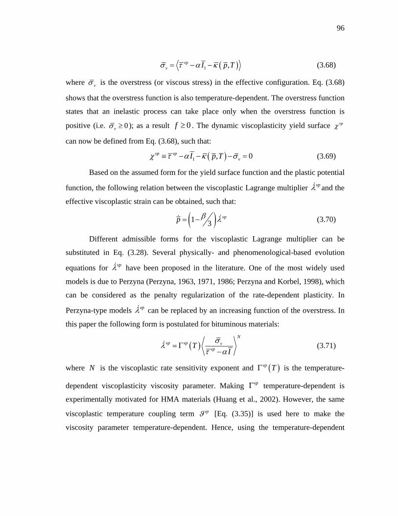
96
1 ,vpv I p T (3.68)
where v is the overstress (or viscous stress) in the effective configuration. Eq. (3.68)
shows that the overstress function is also temperature-dependent. The overstress function
states that an inelastic process can take place only when the overstress function is
positive (i.e. 0v ); as a result 0f . The dynamic viscoplasticity yield surface vp
can now be defined from Eq. (3.68), such that:
1 , 0vp vpvI p T (3.69)
Based on the assumed form for the yield surface function and the plastic potential
function, the following relation between the viscoplastic Lagrange multiplier vp and the
effective viscoplastic strain can be obtained, such that:
1 3vpp (3.70)
Different admissible forms for the viscoplastic Lagrange multiplier can be
substituted in Eq. (3.28). Several physically- and phenomenological-based evolution
equations for vp have been proposed in the literature. One of the most widely used
models is due to Perzyna (Perzyna, 1963, 1971, 1986; Perzyna and Korbel, 1998), which
can be considered as the penalty regularization of the rate-dependent plasticity. In
Perzyna-type models vp can be replaced by an increasing function of the overstress. In
this paper the following form is postulated for bituminous materials:
N
vp vp vvp
TI
(3.71)
where N is the viscoplastic rate sensitivity exponent and vp T is the temperature-
dependent viscoplasticity viscosity parameter. Making vp temperature-dependent is
experimentally motivated for HMA materials (Huang et al., 2002). However, the same
viscoplastic temperature coupling term vp [Eq. (3.35)] is used here to make the
viscosity parameter temperature-dependent. Hence, using the temperature-dependent
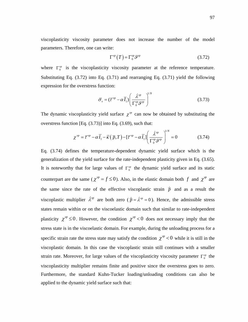
97
viscoplasticity viscosity parameter does not increase the number of the model
parameters. Therefore, one can write:
0vp vp vpT (3.72)
where 0vp is the viscoplasticity viscosity parameter at the reference temperature.
Substituting Eq. (3.72) into Eq. (3.71) and rearranging Eq. (3.71) yield the following
expression for the overstress function:
1/
10
( )Nvp
vpv vp vp
I
(3.73)
The dynamic viscoplasticity yield surface vp can now be obtained by substituting the
overstress function [Eq. (3.73)] into Eq. (3.69), such that:
1/
1 10
, [ ] 0Nvp
vp vp vpvp vp
I p T I
(3.74)
Eq. (3.74) defines the temperature-dependent dynamic yield surface which is the
generalization of the yield surface for the rate-independent plasticity given in Eq. (3.65).
It is noteworthy that for large values of 0vp the dynamic yield surface and its static
counterpart are the same ( 0vp f ). Also, in the elastic domain both f and vp are
the same since the rate of the effective viscoplastic strain p and as a result the
viscoplastic multiplier vp are both zero ( 0vpp ). Hence, the admissible stress
states remain within or on the viscoelastic domain such that similar to rate-independent
plasticity 0vp . However, the condition 0vp does not necessary imply that the
stress state is in the viscoelastic domain. For example, during the unloading process for a
specific strain rate the stress state may satisfy the condition 0vp while it is still in the
viscoplastic domain. In this case the viscoplastic strain still continues with a smaller
strain rate. Moreover, for large values of the viscoplasticity viscosity parameter 0vp the
viscoplasticity multiplier remains finite and positive since the overstress goes to zero.
Furthermore, the standard Kuhn-Tucker loading/unloading conditions can also be
applied to the dynamic yield surface such that:

98
0,vp 0,vp 0,vp vp 0vp vp (3.75)
Moreover, the dynamic yield surface can expand and shrink due to both
softening/hardening effects and softening/hardening rate effects. The non-associative
viscoplasticity flow rule can now be obtained by substitute Eqs. (3.71) and (3.72) into
Eq.(3.28), such that:
0
Nvp vp vp v
ij vpij
F
I
(3.76)
Eqs. (3.74) and (3.76) show that the viscoplastic temperature coupling term should be
included in both the flow rule and the dynamic viscoplasticity yield surface.
3.6. Viscodamage Constitutive Model
In this work, the constitutive models are expressed in the effective stress space. In this
section, the thermo-viscodamage model will be formulated and will be coupled to the
thermo-viscoelastic and thermo-viscoplastic models. Therefore, expressing the
viscodamage model elements (i.e. the damage potential function G and damage surface
function g ) in the effective stress space seems quiet natural since damage also affects
the undamaged skeleton of material. The damage force can be derived from the
Helmholtz free energy function by substituting Eq.(3.36) into Eq. (3.15), such that:
1
1 211 exp
tvdvd vd
eff
bY I b T
(3.77)
An analogous procedure for formulating the viscoplastic model is used to formulate
the viscodamage model. In this work the damage growth surface g is assumed to be the
same as the damage potential function G (i.e. associative viscodamage). One can define
a very simple static damage loading surface, such that:
0 0g Y Y (3.78)
where Y is the damage force [Eq. (3.77)] and 0Y is the threshold damage force. Very
similar to the viscoplasticity, one can extend Eq. (3.78) to include the rate-dependent
damage (viscodamage) such that:
99
0vd vdvg (3.79)
where vd is the dynamic damage loading surface and vdv is the damage overstress
defined as:
0vdv Y Y (3.80)
A form similar to the form selected for the admissible viscoplastic Lagrange multiplier is
postulated for the damage Lagrange multiplier vd . Hence, the following form which is
an increasing function of the damage overstress is postulated for the damage Lagrange
multiplier:
0
0
qvdvd vd v Y
Y
(3.81)
where vd is the damage viscosity parameter and q is a material constant. From Eq.
(3.81) one can simply determine the damage overstress as:
1
0 1qvd
vdv vd
Y
(3.82)
Substituting Eq. (3.78) into Eq. (3.27) implies that the damage multiplier vd is the same
as the damage rate (i.e. vd ). Finally, the dynamic viscodamage loading surface can
be obtained by substituting Eqs. (3.77) and (3.78) into Eq. (3.79), such that:
1
0 0q
vdvd
Y Y
(3.83)
Substituting Eq. (3.77) into Eq. (3.83) yields:
1
1
1 2 011 exp 0
qvd vd vd
eff vd
bI b Y
(3.84)
The temperature-dependent dynamic viscodamage loading function, 0vd , defined in
Eq. (3.84) is the generalization of its static counterpart 0g [Eq. (3.78)]. Similar to the
viscoplasticity loading surface, the static damage loading surface can be recovered for
large values of the damage viscosity parameter vd . In the undamaged domain g and
100
vd are the same since there is no damage evolution (i.e. 0vd ). In this case the
allowable stress states are forced to remain on or within the viscoelastic domain, so that
one has similar to rate-independent damage 0g . Again analogous to the
viscoplasticity, during the unloading process and for a particular damage rate, 0vd
does not necessarily imply that the material is in the undamaged domain, but the material
could still be in the damage state with a smaller damage rate. The generalized Kuhn-
Tucker loading/unloading conditions can also be applied to the dynamic viscodamage
surface, such that:
0,vd 0,vd 0,vd vd 0vd vd (3.85)
The evolution law for the thermo-viscodamage model can be obtained by rearranging
Eq. (3.84), such that:
1
1
20
11exp
qvd
qvd vdeff
bI
b qY
(3.86)
where the viscodamage temperature coupling term can be defined as:
10
exp 1qvd vd T
T
(3.87)
As explained in the previous chapter, the proposed viscodamage model has the
advantage that allows a systematic and straightforward procedure for determination of
unique model parameters which makes its calibration very simple.
3.7. The Heat Equation
Bituminous materials and asphalt mixes are temperature- sensitive materials. Asphalt
mixes are subjected to thermal loadings due to the daily and seasonal fluctuations in
temperature during their service life. Also, some specific phenomena such as compaction
of hot mix asphalt in the field are associated with drastic temperature changes.
Moreover, local temperature changes because of the energy dissipation associated with
the deformation processes influence the mechanical properties of asphalt mixes. Hence,
including the temperature evolution in the constitutive model seems inevitable for

101
accurate modeling of the mechanical response of asphalt mixes. In this subsection, the
heat equation is derived.
Substituting the internal energy per unit mass, e , from Eq. (3.6) into the first law
of thermodynamics [Eq. (3.4)] for the effective configuration implies the following
energy balance equation:
, 0ij ij ext i iT T r q (3.88)
Substituting from Eq. (3.9) into the above energy balance equation and making use
of results in Eqs. (3.13), (3.14), (3.15), (3.16), and (3.30) yield the following equation:
( ) ( ),
vp m mij ij ext i iT Q p Y r q (3.89)
On the other hand, Substituting Eqs. (3.19), (3.20), (3.21), and (3.30) into Eq. (3.89)
gives:
,ve vp vd
ext i iT r q (3.90)
Looking at Eqs. (3.41), (3.42), (3.43), and (3.44) reveals that:
( ), , , ,ve mij p T (3.91)
Taking the time derivative of Eq. (3.91) yields:
( )( )
ve mijve m
ij
p Tp T
(3.92)
Substituting Eq. (3.92) into Eq. (3.90) yields the thermo-mechanical heat balance
equation, such that:
( )
( ),
Thermo-mechanical coupling terms
mijve vp vd m ve
p ij ext i i
Q Yc T p T r q
T T T T
(3.93)
where pc T T is the tangent specific heat capacity at constant pressure. Therefore,
from the above equation, one can calculate the increase in temperature associated with
the energy dissipation during the viscoelastic, viscoplastic, and viscodamage
deformation processes, and due to the external heat sources and conduction.
The thermo-mechanical terms in Eq. (3.93) can be obtained using Eqs. (3.44),
(3.46), (3.52), (3.53), (3.57), (3.66), and (3.77), such that:

102
( )
( )1
mve n ve
ijm ij mn
Qa P P Z
T
(3.94)
(0) (0)
(2)(1) ( )
0
( ) ( ) exp
ij ve veijtu tukl kl
vevem kl
ijtu tukl m mve
G E ZT
d gZG E d
d
(3.95)
0 1 21 exp( ) vpp ZT
(3.96)
1
1 211 expvd vd
eff
bYI b Z
T
(3.97)
where Z T . The heat flux vector, q , can also be determined using the well-
known Fourier’s heat conduction law, such that:
i ij jq k T (3.98)
By substituting Eqs. (3.52), (3.94), (3.95), (3.96), (3.97), and (3.98) into Eq.
(3.93) one realizes that the right hand side of thermo-mechanical heat balance [Eq.
(3.93)] becomes a function of viscoelastic strain tensor, veε , effective viscoplastic
strain, p , damage density, , and temperature, T . Eq. (3.93) expresses the changes in
the temperature during the deformation processes.
3.8. Conclusions
In this work, a systematic and consistent thermodynamic-based framework for
constructing a temperature-, time-, and rate-dependent constitutive model for bituminous
materials, which provides a coupling among temperature, viscoelasticity, viscoplasticity,
and viscodamage, is presented.
The viscodamage model is coupled to other parts of the constitutive model by
using the concept of the effective (undamaged) configuration within the continuum
damage mechanics framework. Hence, the Helmholtz free energy function is expressed
in terms of the internal state variables in the effective configuration.

103
This thermodynamic framework which is based on the Clausius-Duhem
inequality is used to derive the constitutive models presented in Chapter II. It is shown
that the presented constitutive model is thermodynamically consistent.
However, as mentioned in Chapter II, the presented constitutive model does not
include the micro-damage healing effect which makes the constitutive model unable to
predict reasonable responses in the presence of the rest period. This very crucial issue
will be discussed for general cases in Chapter IV and for the asphalt mixes in Chapter V.

104
CHAPTER IV
A CONTINUUM DAMAGE MECHANICS FRAMEWORK FOR
MODELING MICRO-DAMAGE HEALING
4.1. Introduction
Followed by Kachanov (1958) pioneering work on continuum damage mechanics, many
researchers have used the effective configuration concept to model the irreversible
damage processes in engineering materials. However, experimental observations in the
last decade have clearly shown that various classes of engineering materials such as
polymers, biomaterials, and asphalt binder have the potential to heal and retrieve part of
their strength and stiffness under specific conditions.
The intrinsic healing capability of biomaterials and biological systems is a well-
known and well-established fact (e.g. Yasko et al., 1992; Rodeo et al., 1993; Arrington
et al., 1996; Strauer et al., 2002; Werner and Grose, 2003). Moreover, several procedures
for synthesizing self-healing polymers are recently developed inspired by these unique
features of biological systems and materials (e.g. White et al., 2001; Brown et al., 2005;
Bond et al., 2007; Rong et al., 2007; White et al., 2008; Yin et al., 2008; Yuan et al.,
2008). Another category of the engineering materials that tend to heal is the composite
materials whose matrix is intrinsically tend to heal at elevated temperatures and during
the rest periods (Little and Bhasin, 2007; Bhasin et al., 2008; Bhasin et al., 2011).
Interestingly, from the continuum point of view, the common feature of the healing
phenomenon in all of these materials (e.g. self-healing polymers and biomaterials) is that
the induced micro-damages (e.g. micro-cracks, micro-voids) gradually reduce in size and
subsequently cause the material to recover partially or fully its strength and stiffness.
Therefore, it seems quite natural to relate the modeling of the healing phenomenon to the
size and density of the healed micro-damages.
The common modeling practice in predicting the damage evolution and growth
in the context of continuum damage mechanics is to treat the damage nucleation and
growth analogously to time-independent plasticity by introducing a damage surface

105
(analogous to the yield surface) which determines the damage nucleation criterion and a
damage evolution function which quantifies the damage density (Kachanov, 1986;
Lemaître and Chaboche, 1990; Voyiadjis and Kattan, 1990; Krajcinovic, 1996). This
modeling treatment of continuum damage mechanics yields to the fact that damage does
not evolve during the unloading where the material point is located in the damage
loading surface. Subsequently, the stiffness modulus remains constant during the
unloading resulting in a linear response in the stress-strain diagram during the unloading.
Figure 4.1 shows a schematic representation of the stress-strain response for a complete
unloading-loading cycle (e.g. Karsan and Jirsa, 1969).
Figure 4.1. Schematic representation of the stress-strain response for a loading (path “AB”), unloading (Path “BC”), and reloading (path “CD”) cycle. The stress-strain response during the
unloading is nonlinear and also the tangent stiffness at the end of the unloading (i.e. UL,t CE ) is less
than the tangent stiffness modulus at the beginning of the reloading (i.e. ReL,t CE ).
As shown schematically in Figure 4.1 and has also been reported in numerous
experimental studies on engineering materials, the stress-strain response during the
unloading [path “BC” in Figure 4.1] is nonlinear (e.g. Sinha et al., 1964; Karsan and
B
C
D
A
ReL,t CE
UL,t CE

106
Jirsa, 1969; Ortiz, 1985; Bari and Hassan, 2000; Mirmiran et al., 2000; Eggeler et al.,
2004; Palermo and Vecchio, 2004; Sima et al., 2008).
In this work, the nonlinear response of the stress-strain diagram during the
unloading is related to extra damage growth during the unloading. It should be noted that
Ortiz (1985) was the first to model the nonlinear response of the stress-strain diagram
during the unloading by considering the anisotropic damage and crack closure. In this
work, the damage anisotropy is not included; instead, the damage function is allowed to
evolve with a slower rate during the unloading to model this distinct behavior.
Moreover, the arguments in the subsequent sections show that the underlying
assumptions of this work are physically in line with the fundamental assumptions of
Ortiz (1985).
Moreover, the experimental observations on cyclic loading of several materials
show a jump in the tangent stiffness modulus at the unloading-loading points [point “C”
in Figure 4.1] (Sinha et al., 1964; Karsan and Jirsa, 1969; Ortiz, 1985; Hassan et al.,
1992; Eggeler et al., 2004; Sima et al., 2008). In other words, as shown schematically in
Figure 4.1, the material recovers part of its stiffness at unloading-loading point such that
the tangent stiffness at the beginning of the subsequent loading cycle [ ReL,t CE in Figure
4.1] is greater than the tangent stiffness modulus at the end of the unloading [ UL,t CE in
Figure 4.1]. This jump in the tangent stiffness at the unloading-loading point becomes
more significant if rest periods (or unloading times) are introduced between the loading
cycles. The current study shows that this distinct behavior could be related to micro-
damage healing at low strain levels. In other words, at the end of the unloading, the
strain levels becomes close to zero such that the faces of the induced micro-damages wet
each other and retrieve part of their bond strength. The wetting of the micro-damage
surfaces results in partial healing and subsequently partial recovery in the tangent
stiffness modulus at unloading-loading point. This phenomenon is usually referred to as
instantaneous healing (Wool and Oconnor, 1981). More healing will occur (e.g. due to
cohesion and inter-molecular diffusion process between the micro-crack faces in
polymers, biomaterials, and bituminous materials) if the wetted surfaces of the micro-

107
damages put into rest for a while before the next loading cycle is applied. This
phenomenon is usually referred to as the time-dependent (or long-term) healing in the
literature (Wool and Oconnor, 1981).
Several phenomenological-based formulations for describing the healing
phenomena in different materials have been proposed in the literature (e.g. Jacobsen et
al., 1996; Ramm and Biscoping, 1998; Ando et al., 2002). However, little attention is
devoted to the proper coupling of the healing to continuum damage mechanics. Miao et
al. (1995) proposed a constitutive model for compaction of crushed rock salts, Barbero et
al. (2005) proposed a thermodynamic-based continuum damage-healing constitutive
model for self-healing composites, and Voyiadjis et al. (2011) extended the work of
Barbero et al. (2005) by incorporating the isotropic hardening in damage and healing
models. However, more studies are needed to develop a robust and simple computational
technique to model the phenomena associated with the micro-damage healing in
materials that tend to heal. Therefore, this study aims to contribute in filling this gap by
proposing a micro-damage healing framework in the context of the continuum damage
mechanics. The proposed framework introduces a healing configuration which enriches
the continuum damage mechanics theories in modeling the micro-damage healing
phenomenon. The well-known transformation hypotheses of continuum damage
mechanics from the effective (undamaged) to the nominal (damaged) configurations are
extended here to incorporate self-healing. Moreover, analytical relations are derived to
relate the stiffness moduli in different configurations. Several numerical examples are
presented in order to demonstrate the capabilities of the proposed framework in
capturing interesting phenomena such as: (a) the stiffness and strength recovery in cyclic
loading upon the application of rest periods; (b) the nonlinear response of the stress-
strain diagram during unloading; and (c) the jump in the tangent stiffness modulus at the
unloading-loading point (Darabi et al., 2011b).

108
4.2. Micro-Damage Healing Configuration
In the classical continuum damage mechanics (CDM) framework, a scalar variable, the
damage variable, for the case of the isotropic damage or a higher-order tensor, the
damage tensor, for the case of the anisotropic damage is usually used to explain the
degradation behavior of materials due to micro-damage (micro-cracks and micro-voids)
nucleation and growth [see e.g. Voyiadjis and Kattan (1999) for a comprehensive review
of the this subject]. For simplicity and without loss of generality, the case of isotropic
damage is considered here. In this work, the effective (undamaged) configuration is
generalized to the cases when materials undergo micro-damage healing or partial/full
recovery of the damaged stiffness.
Figure 4.2(a) shows a cylinder under a uniaxial tensile load T at the current time
“ t”. During the loading-unloading processes, some new micro-cracks and micro-voids
nucleate and propagate upon satisfaction of the damage nucleation and growth
conditions. On the other hand, for certain materials (e.g. polymers, bituminous materials,
and biological materials) some of these micro-cracks may heal during the resting period
(or the unloading process). Therefore, one can divide the total cross-sectional area, A , of
the cylinder into three parts: (a) the area that has not been damaged (i.e. intact area), A ,
which can be considered as the effective (undamaged) area in CDM; (b) the area of
unhealed cracks and voids, uhA , where damage is considered irreversible; (c) the area of
micro-cracks and micro-voids that have been healed during the unloading process or the
rest period, hA . Figure 4.2(b) shows the cross-sectional area of the cylinder at time “ t”
in the nominal (damaged) configuration. One can assume that the area of the completely
healed micro-damages have the same properties of the intact material. Hence, once a
micro-crack heals completely, it retrieves all of its strength such that its mechanical
properties become identical to those of the intact material. Figure 4.2(c) shows the
healing configuration.

109
(a)
(b) (c) (d) Figure 4.2. Schematic representation of: (a) the damaged partially healed cylinder in tension; (b) the nominal configuration; (c) the healing configuration; and (d) the effective configuration. The
nominal configuration includes the intact material, unhealed damages, and healed micro-damages; the healing configuration includes the intact material and the healed micro-damages
and the effective configuration only includes the intact material.
, ,uhA A A E
Nominal (damaged) configuration
Healing configuration
Effective (undamaged) configuration
, ,A E , ,h uhA A A A E
Remove both healed and unhealed damages (micro-cracks and micro-voids)
Remove healed damages Remove all unhealed damages
Cross section
Healed micro-damages, hA Unhealed micro-damages, uhA T
T

110
This fictitious configuration results when unhealed cracks and voids are removed from
the damaged configuration. The effective (undamaged) configuration is shown in Figure
4.2(d). This fictitious configuration includes the materials that have never been damaged
(intact) during the loading-unloading history. This configuration is identical to the so-
called effective configuration in CDM when healing does not occur. Therefore, one can
write from Figure 4.2:
D uhA A A A A (4.1)
D uh hA A A (4.2)
where A , A , and A are the cross-sectional area in the nominal (damaged), effective
(undamaged), and healing configurations, respectively; and DA is the summation of
both healed micro-cracks and micro-voids, hA , and unhealed micro-cracks and micro-
voids, uhA .
As it is assumed in CDM, cracks and voids cannot carry load. In fact, load is
carried by the area of the intact material and the healed micro-damages. Therefore, one
can assume that the applied forces in the nominal and healing configurations are equal,
such that:
T A A (4.3)
where is the nominal (apparent) stress and is the stress in the healing configuration
(true or net stress). In this paper, the superscripts “ ” and “ ” designate the effective
and healing configurations, respectively. The following definitions are introduced for the
damage and healing internal state variables, respectively:
DA
A (4.4)
h
D
Ah
A (4.5)
For the cases when healing is not considered, is the classical irreversible damage
density variable ranging from 0 1 , which is interpreted as the micro-damage
density such that 0 indicates no damage and 1 indicates complete damage (or

111
fracture). However, when healing is included, is interpreted as an internal state
variable representing the damage history such that DA is the accumulative damaged
area. On the other hand, h is the healing internal variable defined as the ratio of the
accumulative area of healed micro-damages over the accumulative damaged area.
Therefore, h represents the healed fraction of the total accumulative damaged area. The
healing variable ranges from 0 1h ; 0h for no healing and 1h when all micro-
cracks and micro-voids are healed.
Substituting Eqs. (4.1), (4.2), (4.4), and (4.5) into Eq. (4.3) yields:
1
(4.6)
where is the effective damage density ranging from 0 1eff , such that:
1 h (4.7)
such that 0 indicates that either the material has not been damaged yet or all induced
damages have already been healed; whereas, 1 indicates complete damage (or
fracture). It should be noted that the effective damage density variable is no longer
irreversible and can decrease upon micro-damage healing.
It is noteworthy that the healing variable in Eq. (4.7) has a similar effect to the
stiffness-recovery parameter introduced in the work of Lee and Fenves (1998) for
modeling the stiffness recovery in concrete materials during the transition from tension
to compression loading. However, the physics behind the stiffness-recovery parameter
by Lee and Fenves (1998) is different than the current proposed micro-damage healing
variable h . Lee and Fenves (1998) interpreted the area of healed micro-cracks in Eq.
(4.5), hA , as the area of closed micro-cracks (not healed) during the loading transition
from tension to compression. Therefore, the current proposed healing variable is more
general as it can be interpreted as a crack-closure parameter or as a healing parameter,
but with a different evolution law, depending on the intended application.
Eqs. (4.6) and (4.7) relate the stress in the healing configuration to the nominal
stress as a function of the damage and healing internal variables. This expression

112
represents the proper coupling between the damage and healing variables and modifies
the classical definition of the effective stress in CDM [i.e. / (1 ) when
healing is not considered (i.e. 0h )].
Eq. (4.6) can be simply generalized for three-dimensional cases for the case of
the isotropic (scalar) damage, such that:
1 (1 )1 h
(4.8)
where is the nominal stress tensor in the damaged configuration and is the true
stress tensor in the healing configuration.
Moreover, the following relationship between the stress tensors in the healing
and effective configurations will be obtained if one assumes that the tensile forces in the
effective and healing configurations are the same (i.e. A A in Figure 4.2), such
that:
1 1
1
h
(4.9)
Eq. (4.9) clearly shows that the stress tensors in the healing and effective configurations
will be the same only for two cases: (1) damage variable is zero (i.e. 0 ), where in
this case the stress tensors in the effective and healing configurations (i.e. and ) will
be the same as the stress tensor in the nominal configuration (i.e. ) since damage has
not started yet; (2) healing variable is zero (i.e. 0h ), where in this case the stress
tensors in the effective and healing configurations will be the same since healing is not
considered. For other cases, the stress tensor in the fictitious effective configuration will
be always greater than the stress tensor in the healing configuration (i.e. ). In other
words, the effective configuration (Figure 4.2(d)) is obtained by removing the healed
micro-damage areas from the healing configuration (Figure 4.2(c)) such that these
healed micro-damages can tolerate load and carry stress in the healing configuration.
Therefore, the stress tensor in the effective configurations should be magnified
comparing to the stress tensor in the healing configuration in order to compensate for the
stresses carried by the removed healed micro-damages.

113
In the above, the relations between the stresses in different configurations are
derived. In the following sections, the relations among the strain tensors and stiffness
moduli in different configurations will be derived.
4.3. The Stiffness Moduli in Different Configurations
As mentioned in previous Section, completely healed micro-cracks and micro-voids
recover their total strength and stiffness such that they become identical to the intact
material. Hence, one can assume that the stiffness moduli in the effective and healing
configurations are the same and equal to the stiffness modulus of the virgin state of the
material that does not change during the loading-unloading history, such that:
t tE E (4.10)
where tE and tE are the tangent stiffness moduli in the effective and healing
configurations, respectively. The tangent stiffness modulus is used in this paper instead
of the commonly used secant stiffness modulus in CDM theories. The nominal tangent
stiffness modulus is defined as:
t
d
dE
(4.11)
The secant stiffness modulus is commonly used in CDM to capture the degradation of
the stiffness modulus with damage evolution. However, the tangent stiffness modulus
could capture the nonlinear response of materials easier and is commonly used instead of
the secant stiffness modulus for the numerical implementation purposes. Figure 3
schematically illustrates the advantages of using tangent stiffness modulus rather than
the secant stiffness modulus. Figure 4.3 shows three different paths that point “A” may
continue on the stress-strain curve. Path (1) represents a path on which the material
shows hardening behavior; the material goes to the softening region on path (2); and
path (3) represents a schematic unloading path. The secant stiffness modulus of point
“A” (i.e. AE ) will be the same for all these three different paths as shown in Figure 4.3.
However, the tangent stiffness modulus at point “A” for each of these paths will be
different (i.e. , ,1t AE , , ,2t AE , and , ,3t AE corresponding to paths (1), (2), and (3),

114
respectively). Therefore, these different paths will clearly be distinguished by looking at
the tangent stiffness moduli at point “A”. Moreover, physically speaking, a material
point at a specific time feels the tangent stiffness modulus as the measure of its stiffness.
In other words, if the tangent modulus at an arbitrary point “c” on the stress-strain curve
is greater than that of point “d”, it can simply be implied that the material has the
capacity to build up larger stress increment at point “c” rather than point “d” for the
same strain increment. However, this simple argument cannot be made by looking at the
values of the secant modulus at those points unless the history of the secant modulus is
studied [please see Eq. (4.15)].
Figure 4.3. Schematic illustration of three possible paths for point “A” on the stress-strain curve. Path (1) represents the path on which the material shows hardening behavior; material point goes
to softening region on path (2), and path (3) represents a schematic unloading path. The secant stiffness modulus of point “A” will be the same for all these three paths. However, these paths can be distinguished by looking at the tangent stiffness modulus of point “A” for each stress-
strain path.
However, one can simply derive the relationship between the tangent and secant
stiffness moduli as illustrated in the following developments. For the secant stiffness
modulus, one can write:
σ E : ε= (4.12)
A
AE
(1)
(2)
(3)
, ,1t AE
, ,2t AE
, ,3t AE

115
where , , hE E E is the fourth-order damaged-healed secant stiffness tensor, and
is the strain tensor in the nominal configuration. Taking the time derivative of Eq. (4.12)
yields:
-1σ = E : ε + E : ε = E + E : εε : ε (4.13)
The superimposed dot in this equation and all subsequent equations indicates derivative
with respect to time. Also, “A-1” indicates the inverse of “A”. On the other hand, for the
tangent stiffness modulus, one can write:
tσ E : ε = (4.14)
The relation between the tangent and secant moduli is obtained by comparing Eqs. (4.13)
and (4.14), such that:
1:t E E E (4.15)
Different expressions for E are derived next based on adapting three different
transformation hypotheses to relate the healing configuration to the damaged
configuration.
As argued before, the stiffness moduli in the effective and healing configurations
are the same [Eq. (4.10)] and do not change during the loading-unloading history or as
the material damages or heals. Hence, one can simply imply that for elastic-damage-
healing materials, the secant and tangent stiffness moduli in both effective and healing
configurations are the same as the initial undamaged stiffness modulus of the intact
materials, such that:
t t E E E E (4.16)
Moreover, stress and strain tensors and their rates are related through the following
relationships:
E : ; t E : (4.17)
Taking the time derivative of Eq. (4.8) yields:
1 (1 )h h h (4.18)

116
Now, several transformation hypotheses from the healing configuration to the
damage configuration are discussed. It should be noted that Eqs. (4.9) and (4.16) relate
the stress tensors and stiffness moduli in the effective and healing configurations. One
can also establish a general relationship between the strain tensors in the effective and
healing configurations. Eq. (4.16) yields:
1 1 E E (4.19)
Substituting Eq. (4.9) into Eq. (4.19) gives:
1 1
1
h
(4.20)
Eq. (4.20) relates the strain tensors in the effective and healing configurations and shows
that these two tensors will be the same when healing is not included (i.e. 0h ) or when
there is no damage (i.e. 0 ). Otherwise, there will be differences between the strain
tensors in the effective and healing configurations depending on the levels of damage
and healing. Also, Eq. (4.20) is true independent of the following postulated
transformation hypotheses.
In the next sub-sections, the relationships between the strain tensors and stiffness
moduli in the nominal (damaged) and healing configurations will be established for
different transformation hypotheses. Relations between the stress tensors, stiffness
moduli, and strain tensors in the healing and effective configurations can evidently be
obtained using Eqs. (4.9), (4.16), and (4.20), respectively.
4.3.1. Strain Equivalence Hypothesis
The first commonly used hypothesis in CDM to relate the nominal stress and strain
tenors ( and ) to the stress and strain tensors in the undamaged effective
configuration ( and ) is the strain equivalence hypothesis which states that the strain
tenors in the nominal and effective configurations are equal (Lemaître and Chaboche,
1990). This is the simplest transformation hypothesis that one can think about and makes
the theoretical derivation and numerical implementation of constitutive models relatively
easier. However, this hypothesis is inaccurate in case of large deformations and/or

117
significant damage evolution. This hypothesis is extended here for the healing
configuration such that one can assume that the strain tensors in the nominal and healing
configurations are equal, such that:
(4.21)
It should be noted that equivalency of the strain tensors in the healing and
nominal configurations does not imply the equivalency of the strain tensors in the
effective and healing configurations when healing is included. In fact, Eq. (4.20) relates
the strain tensors in the healing and effective configurations when healing is included.
Substituting Eq. (4.18) into 1tε E : σ = [Eq. (4.14)] yields:
1 11 (1 ) t th h h ε E : σ + E : σ = (4.22)
Substituting Eq. (4.17)2 into Eq. (4.22) yields:
1 11 (1 ) t t t th h h ε E : E : ε E : E : ε (4.23)
Furthermore, substituting Eq. (4.21) into Eq. (4.23) gives:
11 1 :t th h h E E (4.24)
Eq. (4.24) expresses the changes in the nominal tangent stiffness as a function of the
damage variable, the healing variable, the strain level, and their rates. As will be shown
in the subsequent developments, Eq. (4.24) is able to capture the nonlinear response of
the material during the loading as well as the unloading processes. Another feature of
Eq. (4.24) is that it takes into account the deformation history by including the strain
level. This equation can also capture the changes in the stiffness modulus at the loading-
unloading point in the cyclic loading which is triggered by the presence of the strain rate
in Eq. (4.24).
One can also simply derive the relation between the secant stiffness modulus and
its rate in the nominal and healing configurations by substituting Eqs. (4.12), (4.17)1, and
(4.21) into Eq. (4.8), such that:
1 1 h E E (4.25)

118
Taking the time derivative of Eq. (4.25) and noting that the secant modulus in the
healing configuration is constant (i.e. 0E ) imply:
h h E E (4.26)
Eqs. (4.25) and (4.26) relate the secant stiffness modulus and its rate in the nominal
configuration to their corresponding counterparts in the healing configuration. It should
be noted that Eq. (4.24) can be derived simply by substituting Eqs. (4.16), (4.25), and
(4.26) into Eq. (4.15).
4.3.2. Elastic Strain Energy Equivalence Hypothesis
Another commonly used transformation hypothesis in CDM is the elastic strain energy
equivalence hypothesis (Cordebois and Sidoroff, 1982; Voyiadjis and Kattan, 1993;
Lemaître et al., 2000), which is more physically sound comparing to the strain
equivalence hypothesis (Abu Al-Rub and Voyiadjis, 2003). The elastic strain energy
densities in the nominal and healing configurations for the elastic-damage-healing
materials can be written as follows:
1
2W : ;
1
2W : (4.27)
The elastic strain energy equivalence hypothesis states that the elastic strain energy
densities in the nominal and effective configurations are the same (i.e. the elastic strain
energy is stored in the intact material). This hypothesis is postulated here for the nominal
and healing configurations, such that:
W W (4.28)
However, this hypothesis does not imply the equivalency of the elastic strain energy in
the nominal and effective configurations when healing is included. The relationship
between the elastic strain energies in the effective, nominal, and healing configurations
can be obtained using Eqs. (4.9), (4.20), and (4.28), such that:
2
1
1 1W W W
h
(4.29)

119
where 2W : . Eq. (4.29) shows that the elastic strain energy in the effective
configuration will be equivalent to that in the nominal and healing configurations only
when the healing variable is zero (i.e. healing is not included) or when there is no
damage. Substituting Eqs. (4.8) and (4.27) into Eq. (4.28) yields:
1 1 h (4.30)
Eq. (4.30) relates the strain tensors in the nominal and healing configurations. The
relationship between the tangent moduli in the nominal and healing configurations can
then be obtained by substituting Eqs. (4.12), (4.14), (4.16), (4.17), and (4.30) into Eq.
(4.18), such that:
2 11 1 2 1 1t th h h h E : E (4.31)
Furthermore, the relations between the secant stiffness modulus and its rate in the
nominal and healing configurations can be derived by substituting Eqs. (4.12), (4.16),
(4.17)1, and (4.30) into Eq. (4.8), such that:
21 1 h E E (4.32)
2 1 1h h h E E (4.33)
Equivalently, substituting Eqs. (4.32) and (4.33) into Eq. (4.15) confirms Eq. (4.31).
4.3.3. Power Equivalence Hypothesis
Another transformation hypothesis to relate strains and stiffness moduli in the nominal
and effective configurations in the absence of micro-damage healing is the power
equivalence hypothesis. This hypothesis has been used by several researchers to derive
constitutive models associated with dissipative processes such as viscoelasticity and
viscoplasticity. To name a few, Lee et al. (1985), Voyiadjis and Thiagarajan (1997), and
Voyiadjis et al. (2004) used this hypothesis to couple damage to plasticity and/or
viscoplasticity models. This hypothesis is extended here to the healing configuration
(instead of the effective configuration) such that one can assume that the power
expenditures in the nominal and healing configurations are the same. This hypothesis is
attractive for mechanisms associated with dissipation processes since the correct

120
estimation of the dissipated energy is generally needed. It is noteworthy that using the
power equivalence hypothesis along with the concept of the stress in the healing
configuration is both numerically and physically interesting. Using the concept of the
stress in the healing configuration eliminates numerical complexities associated with
direct coupling between the damage and healing constitutive equations and at the same
time makes these simplifications physically sound since it allows the accurate estimation
of the dissipated energy in the healing configuration.
The power expenditures in the nominal and healing configurations can be written
as:
1
2 σ : ε ; 1
2 σ : ε (4.34)
Power equivalence hypothesis states that the power expenditure in the nominal, , and
healing, , configurations are the same, such that:
(4.35)
Substituting Eqs. (4.8) and (4.34) into Eq. (4.35) yields:
1 (1 )h ε ε (4.36)
which relates the rate of the nominal strain tensor to its rate in the healing configuration.
Substituting from Eq. (4.8) along with ε from Eq. (4.14) into Eq. (4.34)1 gives:
111 (1 )
2 th σ : E : σ (4.37)
Substituting Eqs. (4.16), (4.17)2, and (4.18) into Eq. (4.37) gives:
2 1
1
11 (1 )
21
1 (1 ) ( )2
t t
t t
h
h h h
σ : E : E : ε
σ : E : E : ε
(4.38)
Using the power equivalence hypothesis [Eq. (4.35)] along with Eqs. (4.34) and (4.38),
one obtains the following expression for the tangent moduli:
2 11 1 1 1 :t th h h h E ε ε E (4.39)

121
The expressions in Eqs. (4.24), (4.31), and (4.39) show different relations
between the tangent moduli in the nominal and healing configurations when different
transformation hypotheses are postulated. Note that the right-hand-side of Eq. (4.39) is
expressed as a function of the strain tensor, ε , and its rate, ε , in the healing
configuration. One may still represent the right-hand-side of Eq. (4.39) as a function of
the strain tensor in the nominal configuration by using Eq. (4.36), such that:
0
1 (1 )t
h dt ε ε (4.40)
Applying the integration by parts to Eq. (4.40) implies:
0
1 (1 )t
h h h dt ε ε ε (4.41)
Eqs. (4.30) and (4.41) show that postulating the power equivalence hypothesis yields a
more general relationship between the strain tensors in the nominal and healing
configurations as compared to the relations obtained by postulating the elastic strain
energy or strain equivalence hypotheses. The difference between Eqs. (4.30) and (4.41)
will be negligible for very slow processes where rate of the healing and damage
variables are close to zero. Otherwise, there will be significant difference between these
two expressions. Eq. (4.39) can now be expressed in terms of the nominal strain tensor
by substituting Eqs. (4.36) and (4.41) into Eq. (4.39), such that:
2
1
1
0
1 1 : 1 1
:
t
t
t
h h h h
h h h h dt
E
E
(4.42)
Furthermore, the relationship between the secant stiffness moduli in the nominal
and healing configurations can be obtained by substituting Eqs. (4.12), (4.17)1, and
(4.41) into Eq. (4.8), such that:
2 1
01 1 1 1 :
th h h h dt E E (4.43)
Moreover, taking the time derivative of Eq. (4.43) yields:

122
1
0
1 1
0
1 1 :
1 1 : : :
t
t
h h h h h h h dt
h h h dt
E
E
(4.44)
Eqs. (4.39) and (4.42) show the expressions for relating the damaged (nominal)
tangent stiffness modulus to the stiffness of the intact material as a function of the
damage density, healing variable, strain, and their rates. These relations can be used to
capture the nonlinear change in the stiffness during the unloading since during the
unloading both the strain and the healing variable change. Furthermore, the presence of
the strain rate enriches Eqs. (4.24), (4.31), and (4.39) to capture the changes in the
stiffness modulus of the loading-unloading point in the cyclic loading. These important
features of these equations will be shown in the following section in order to show the
capabilities of the model in cyclic loading.
4.4. Damage and Healing Models and the Numerical Implementation
4.4.1. Damage and Healing Evolution Functions
Several examples are presented in this section to show the capabilities of the proposed
healing framework in capturing the nonlinear response of materials under cyclic loading.
Recently, Darabi et al. (2011c) and Abu Al-Rub et al. (2010a) have proposed and
validated rate-dependent damage (viscodamage or delay-damage) and healing models,
respectively, and coupled those to viscoelasticity and viscoplasticity constitutive models
to predict the mechanical response of bituminous materials. Simplified forms of these
models are used in this work to investigate the effect of the healing on the mechanical
response of elastic-damage-healing materials. The simplified form of the rate-dependent
damage evolution function in the healing configuration (viscodamage) is given as
follows (Darabi et al., 2011c):
21 exp( )vd
effth
Yk
Y
(4.45)
123
where vd is the viscodamage viscosity parameter that controls how fast damage
nucleates and grows, k is a material constant, eff ij ij is the effective (or
equivalent) strain, thY is the threshold damage force, and Y is the damage driving force
which is assumed to have the following simple form (Darabi et al., 2011c):
2Y J (4.46)
where 12 2 ij ijJ s s is the second invariant of the deviatoric stress in the healing
configuration with 13ij ij kk ijs being the deviatoric stress and ij being the
Kronecker delta.
The presented viscodamage model in Eq. (4.45) can be treated analogous to
viscoplasticity models such that the damage variable evolves when the material state is
on or outside the viscodamage surface. The viscodamage surface can simply be extracted
from the damage evolution function, Eq. (4.45), such that:
21 exp( ) 0vd
th effvdf Y Y k
(4.47)
where vdf is the viscodamage loading surface [please refer to Darabi et al. (2011c;
2011d) for more details]. Hence, the damage variable evolves when the viscodamage
surface is equal or greater than zero.
Since the main aim of this section is to show qualitative effects of micro-damage
healing on responses of elastic-damage-healing materials, a simple phenomenological-
based healing evolution function is adapted (Abu Al-Rub et al., 2010a), such that:
1 1ahh h
(4.48)
where h is the healing viscosity parameter controlling the rate of the micro-damage
healing, and a is a material parameter. The following initiation condition is also
postulated for the healing model:
0h hth efff (4.49)

124
where hf is the healing loading surface, hth is the healing threshold strain, and eff is
the effective strain. Eq. (4.49) assumes that the healing variable evolves when the total
effective strain is smaller than the healing threshold strain. In other words, the healing
occurs at very small strains such that the micro-crack faces are close to each other and
can wet each other in order for healing to occur. Moreover, it should be noted that
healing cannot occur during the damage process and vice versa (i.e. a micro-crack
cannot propagate and heal at the same time; either propagates or heals). Hence, rate of
the healing variable will be zero when damage is evolving (i.e. when 0 ).
In the following subsections, the effect of assuming rate-dependent damage
versus rate-independent damage on the mechanical responses will also be investigated.
Therefore, the following function is assumed to describe the rate-independent damage
model, such that:
exp( )effth
Yk
Y
(4.50)
The main difference between Eq. (4.45) and (4.50) is that the former is time- and rate-
dependent which considers the loading time as well as the loading rate while the later is
time- and rate-independent.
It is noteworthy that the presented models will be used to show qualitative effects
of damage and healing on the mechanical response of elastic-damage-healing materials.
Obviously, the evolution functions for the damage and healing models can be different
for different materials, but similar qualitative trends will be obtained by following the
above formulated continuum damage mechanics framework considering micro-damage
healing.
4.4.2. Numerical Implementation for Different Transformation Hypotheses
The implementation procedure for the presented elastic-damage-healing model using
different transformation hypotheses is discussed in this sub-section. However, as it will
be discussed, the implementation procedure is general and independent of the selected
evolution functions for the damage and healing models.
125
The use of the concept of the stress in the healing configurations substantially
simplifies the numerical implementation of the damage and healing models, especially,
for complex constitutive models where damage and healing models are coupled to
viscoelasticity and/or viscoplasticity models. In other words, one can update the stress
tensor in the healing configuration t t without facing the complexities associated with
the direct couplings of the damage and healing models to the rest of the constitutive
model. The updated stress in the healing configuration can then be used to update the
damage and healing variables and subsequently the nominal stress tensor. It should be
noted that the nominal strain increment tensor t t as well as the nominal total strain
tensor t t at the current time t t are given at the beginning of each increment. The
nominal strain tensor and its increment will be the same as those in the healing
configuration if the strain equivalence hypothesis is used. However, the nominal strain
tensor and its increment will be different from their corresponding values in the healing
configuration if either the elastic strain energy equivalence or the power equivalence
hypotheses are used. Therefore, an iterative scheme is needed to obtain the total strain
and the strain increment tensors in the healing configuration at time t t when the
elastic strain energy equivalence or power equivalence hypotheses are used. The total
nominal strain tensor and its increment at the current time t t , the values of the
internal state variables (i.e. , h , and ) at previous time t , and the stress tensors in the
nominal and healing configurations at previous time t are known. The objective is to
update the current stress tensors in the nominal and healing configurations as well as the
strain tensor in the healing configuration at the current time t t . Hence, one can start
with a trial strain tensor in the healing configuration when the elastic strain energy
equivalence hypothesis is used, such that:
, 1tr t t t t t (4.51)
Similarly, one can start with a trial strain increment in the healing configuration when
the power equivalence hypothesis is used, such that:
, 1tr t t t t t (4.52)

126
Subsequently, the total trial strain tensor in the healing configuration can be obtained for
the power equivalence hypothesis [using Eq. (4.52)], such that:
, ,tr t t t tr t t (4.53)
The trial strain in the healing configuration [Eq. (4.51) for the elastic strain energy
equivalence hypothesis; Eqs. (4.52) and (4.53) for the power equivalence hypothesis]
can then be fed to the Hooke’s law [Eq. (4.17)] to update the stress in the healing
configuration. The next step is to calculate the damage and healing variables based on
the obtained trial strain and stress tensors in the healing configuration. The damage
density can then be obtained by calculating the damage density rate using Eq. (4.45),
such that:
t t t t t t (4.54)
The same procedure can be applied to calculate the healing variable. In other
words, the rate of the healing variable t th (if the healing criterion is met) should be
calculated first using Eq. (4.48). However, as mentioned earlier, healing does not occur
during the damage process and vice versa. Hence, the healed area hA remains constant
during the damage evolution. However, during the healing process both the healing area
hA and the total damage area D h uhA A A which is the summation of the healed and
unhealed damage areas will also evolve. Taking the time derivative of Eq. (4.5) and
making use of Eq. (4.4) yield the following relations for the updated healing variable:
; 0
; 0
tt t t t t
t t
t t t t t t t
h h
h h h t
(4.55)
The new trial strain tensor in the healing configuration will then be recalculated using
updated damage and healing variables. At the end of the iteration, the new and old
values of the strain tensor in the healing configuration will be compared to check the
convergence. Figure 4.4 shows the flowchart for implementation of the presented elastic-
damage-healing constitutive model using different transformation hypotheses.

127
Figure 4.4. A flowchart showing the general finite element implementation procedure of the elastic-damage-healing model using different transformation hypotheses.
Known t , t , t , t , t , th , and t .
Given t t and as a result t t .
Update t t using the trial strain in the healing configuration, Eq. (4.17)
Update damage variable using the updated stress t t [Eqs. (4.45), (4.54)].
t t t t
Set ,t t tr t t .
Calculate the trial strain in the healing configuration
, 1t t tr t t t .
Calculate the trial strain and strain increment in the healing configuration;
, 1t t tr t t t
, ,t t tr t t t tr .
Update healing variable using the updated stress t t [Eqs. (4.48), and (4.55)].
, Tolt t t t tr
Correct the trial strain in the healing
configuration ,t t tr t t .
Elastic strain energy equivalence hypothesis
Strain equivalence hypothesis
Power equivalence hypothesis
Correct the trial strain in the healing
configuration ,t t tr t t
,t t tr t t t .
No No
Yes Yes Yes
Update t t , t t , t t , t th , and t t .
Update the nominal stress tensor t t using Eq. (4.8).
1t t t t t t
t t t t t
,1t t t t t t t

128
4.5. Numerical Results and Examples
The presented elastic-damage-healing model is implemented in the well-known
commercial finite element code Abaqus (2008) via the user material subroutine UMAT.
The finite element model considered here is simply a three-dimensional single element
(C3D8R) available in Abaqus.
4.5.1. Example 1: Different Transformation Hypotheses
The effect of postulating different transformation hypotheses on the mechanical
responses is investigated in this subsection. The rate-dependent damage and healing
models [Eqs. (4.45) and (4.48)] along with the model parameters listed in Table 4.1 are
used for the examples presented in this section.
Table 4.1. Model parameters associated with the presented elastic-damage-healing constitutive model.
E (GPa) vd (s-1) k thY (MPa) h (s-1) a hth
2 0.25 0.25 5 10-7 75 2 0.03 2 0.001
The first simulated example is the uniaxial constant strain rate test (i.e. strain-
controlled uniaxial test). The strain rate is selected as 0.005/sec. The loading history for
this test is shown in Figure 4.5(a). Therefore, during this numerical test, no healing is
expected. The stress-strain responses using different transformation hypotheses are
shown in Figure 4.5(b). Figure 4.5(b) shows that the response of all transformation
hypotheses is close to each other at small strains. However, these responses deviate
when the strain and subsequently the damage density increase. Figure 4.5(b) shows
different responses for the peak point of the stress-strain diagram and the post peak
region in the stress-strain diagram when different transformation hypotheses are
postulated. Furthermore, it shows that the stress-strain response using the power
equivalence hypothesis lies between the numerical results from the strain equivalence
and elastic strain energy equivalence hypotheses.

129
(b) (c)
(d) (e)
Figure 4.5. Model predictions for a uniaxial constant strain rate test using different transformation hypothesis. (a) Loading history; (b) stress-strain responses; (c) ratio of the elastic strain energy in the healing configuration over that in the nominal configuration; (d) ratio of the
expended power in the healing configuration over that in the nominal configuration; and (e) tangent stiffness moduli.
(GPa)tE
-1.5
-1
-0.5
0
0.5
1
1.5
2
0 0.2 0.4 0.6 0.8 1
Strain equivalence hypothesis
Power equivalence hypothesis
Elastic strain energy equivalence hypothesis
Strain equivalence hypothesis
Power equivalence hypothesis
Elastic strain energy equivalence hypothesis
0
1
2
3
4
5
0 0.2 0.4 0.6 0.8
/
/W W
Strain equivalence hypothesis
Power equivalence hypothesis
Elastic strain energy equivalence hypothesis
0
1
2
3
4
5
6
7
8
9
10
0 0.2 0.4 0.6 0.8 1
Strain equivalence hypothesis
Power equivalence hypothesis
Elastic strain energy equivalence hypothesis
0
5
10
15
20
25
30
0 1 2 3 4 5
(%)
MPa
(%)
5
Time (sec) 0 10
(a)

130
The ratio of the elastic strain energy and the expended power in the healing
configuration to their corresponding values in the nominal configuration for different
transformation hypotheses are plotted in Figures 4.5(c) and 4.5(d), respectively. Figure
4.5(c) shows that both the strain equivalence and power equivalence hypotheses predict
higher values for the elastic strain energy in the healing configuration comparing to their
corresponding values in the nominal configuration. However, this deviation is much
significant when the strain equivalence hypothesis is used. On the other hand, Figure
4.5(d) shows that the strain equivalence hypothesis predicts larger values for the
expended power in the healing configuration comparing to its corresponding value in the
nominal configuration; whereas, the elastic energy equivalence hypothesis predicts
lower values for the expended power in the healing configuration comparing to that in
the nominal configuration. However, it should be noted that the main purpose of using
the fictitious healing and/or effective configurations along with a specific transformation
hypothesis is to make the implementation simpler while the underlying physics is
preserved. Also, a proper transformation hypothesis is a one that leads to a constitutive
model that is equivalent when expressed in both the nominal and healing configurations
since both configurations are tools to represent the same material behavior. It is also
interesting to look at this problem from the thermodynamic point of view. As stated by
Ziegler (1977) and have used by many other researchers (Coleman and Gurtin, 1967;
Rice, 1971; Ziegler, 1983; Ziegler and Wehrli, 1987; Fremond and Nedjar, 1996; Collins
and Houlsby, 1997; Shizawa and Zbib, 1999) the constitutive equations for a material
are fully determined by the knowledge of the Helmholtz free energy and a dissipation
function such as the rate of the energy dissipation. Therefore, two systems will be
thermodynamically equivalent if they predict equivalent responses for an energetic
function such as the stored energy and for a dissipative function such as dissipated
power. As shown in Figures 4.5(c) and 4.5(d), none of these hypotheses predict the same
value for both of these two energetic measures (i.e. strain energy and energy power)
functions in nominal and healing configurations. Therefore, qualitative investigation of

131
the responses of each transformation hypothesis is extremely important in deciding the
properness of a specific transformation hypothesis for a specific type of material.
For example, one can use the strain equivalence hypothesis for simplicity if the damage
density is expected to be low. On the other hand, one may use the elastic energy
equivalence hypothesis for the elastic-damage materials where the elastic strain energy
could be the driving force for the damage evolution. Finally, the power equivalence
hypothesis could be used for complex constitutive models including viscoelasticity and
viscoplasticity in which case the elastic strain energy is negligible comparing to the total
strain energy and also the dissipative power and energy becomes of great interest.
Development of a transformation hypothesis that yields to the thermodynamically
equivalent systems in the healing and nominal configurations will be the focus of a
future work by the authors.
Finally, the tangent stiffness moduli for different transformation hypotheses are
plotted in Figure 4.5(e). The negative values of the tangent stiffness modulus show that
the material is in the post peak (softening) region.
The above simulation is repeated for the case of a uniaxial constant stress rate
test as well (i.e. stress-controlled uniaxial test). The loading history, stress-strain
response, the ratio of the elastic energy in the healing and nominal configuration, the
ratio of the power expenditure in the healing and nominal configurations, and the tangent
stiffness using different transformation hypotheses are shown in Figures 4.6(a)-4.6(e),
respectively. Comparing Figures 4.5 and 4.6 yield similar observations for both uniaxial
constant strain rate test and uniaxial constant stress rate test.
The predicted secant stiffness moduli using different transformation hypotheses
are plotted in Figure 4.7 for both uniaxial constant strain rate and uniaxial constant stress
rate tests. Figure 4.7 shows that the predicted secant moduli using the strain equivalence
and elastic strain energy equivalence hypotheses are both path-independent.

132
(b) (c)
(d) (e)
Figure 4.6. Model predictions for a uniaxial constant stress rate test using different transformation hypothesis. (a) Loading history; (b) stress-strain responses; (c) ratio of the elastic strain energy in the healing configuration over that in the nominal configuration; (d) ratio of the
expended power in the healing configuration over that in the nominal configuration; and (e) tangent stiffness moduli.
0
1
2
3
4
0 0.2 0.4 0.6 0.8
Strain equivalence hypothesis
Power equivalence hypothesis
Elastic strain energy equivalence hypothesis
/W W
(GPa)tE
0
0.5
1
1.5
2
0 0.2 0.4 0.6 0.8
Strain equivalence hypothesis
Power equivalence hypothesis
Elastic strain energy equivalence hypothesis
/W W
Strain equivalence hypothesis
Power equivalence hypothesis
Elastic strain energy equivalence hypothesis
0
1
2
3
4
0 0.2 0.4 0.6 0.8
0
5
10
15
20
25
30
0 1 2 3 4 5 6
(%)
Strain equivalence hypothesis
Power equivalence hypothesis
Elastic strain energy equivalence hypothesis
MPa
(MPa)
25
Time (sec) 0 10
(a)

133
This behavior is expected according to Eq. (4.25) and Eq. (4.32) for strain
equivalence and elastic strain energy equivalence hypotheses, respectively. In fact, Eq.
(4.25) shows that the secant stiffness modulus changes linearly as a function of the
damage density for strain equivalence hypothesis; whereas, Eq. (4.32) shows that the
secant stiffness modulus changes quadratic as a function of the damage density when the
elastic strain energy hypothesis is postulated. On the other hand, the secant stiffness
modulus becomes path-dependent when the power equivalence hypothesis is used, as
shown in Figure 4.7.
Figure 4.7. Model predictions of the secant stiffness moduli for both uniaxial constant stress and uniaxial constant strain rate tests using different transformation hypotheses. The secant stiffness
modulus is path-independent when strain equivalence or elastic strain energy equivalence hypotheses are used. However, secant stiffness modulus depends on loading history when the
power equivalence hypothesis is used.
This behavior is also expected by investigating Eq. (4.43). Eq. (4.43). These
equations clearly show that the secant stiffness modulus is a function of the strain and
strain rate in addition to the damage density value when the power equivalence
hypothesis is assumed. This is a very interesting conclusion that needs to be verified
experimentally, which will be the focus of a future work. Such experimental verification
Strain equivalence hypothesis. Both strain control and stress
control tests.
Elastic strain energy equivalence hypothesis. Both strain control
and stress control tests.
Power equivalence hypothesis.
Power equivalence hypothesis.
l
0
0.5
1
1.5
2
0 0.2 0.4 0.6 0.8 1
GPaE

134
will be useful to decide which transformation hypothesis is more physically sound since
this issue is still an open area of research. Many argue that the strain energy equivalence
hypothesis is more physically sound than the strain equivalence hypothesis (e.g.
Lemaitre and Chaboche, 1990; Voyiadjis and Kattan, 1999; Abu Al-Rub and Voyiadjis,
2003). In fact, the current comparison, shows that the power equivalence hypothesis is
more physically attractive since it takes into consideration the loading path-dependency
of damage evolution.
The above examples show how assuming different transformation hypotheses
affect the numerical results. Therefore, each of these transformation hypotheses can be
selected according to the importance of the specific quantities for a specific material. For
example, the strain equivalence hypothesis can be used for simplicity when the damage
density is not expected to have a significant value. The elastic energy equivalence
hypothesis can be used for the elastic-damage materials where the elastic strain energy
could be the driving force for the damage evolution. Finally, one may use the power
equivalence hypothesis for constitutive models with the dissipative nature (such as
viscoelasticity and viscoplasticity) where the elastic strain energy is negligible
comparing to the total strain energy and also the dissipative power and energy becomes
of great interest.
4.5.2. Effect of Healing on Stiffness Recovery
In this subsection, the effect of the healing on the mechanical response of the elastic-
damage-healing materials is investigated. The elastic strain energy equivalence
hypothesis is used in this example since in the current elastic-damage-healing model the
driving force for the damage evolution is related to the elastic strain energy. However,
adapting the other transformation hypotheses will not affect the qualitative results
obtained in this subsection. The rate-dependent damage and healing models are used
[Eqs. (4.45) and (4.48)]. The model parameters used in this section are listed in Table
4.1. The loading history shown in Figure 4.8 can be summarized as follows:
- The material is loaded with a constant strain rate until it is partially damaged (up to
3% strain in this case).

135
- The load is removed with the same rate until the strain reaches zero.
- Material remains in rest for time Rt such that the induced micro-damages can
partially heal. As explained before, Eq. (4.48) is time-dependent. Hence, more
damages will heal for longer rest periods. Therefore different rest periods Rt are
examined to investigate the effect of different healing levels on the stiffness recovery
during the reloading.
- Material is reloaded with the same strain rate until significant amount of damage is
developed.
Figure 4.8. Loading history for the example simulated in Section 4.5.2. Different rest times Rt
are introduced between the loading cycles to investigate the effect of the healing level on stiffness and strength recovery.
Four different rest periods of 0, 50, 200, and 500 sec are assumed in this
example. Figures 4.9(a) and 4.9(b) show the stress-time and stress-strain responses for
different rest periods Rt , respectively. As shown in Figures 4.9and 4.10, the material
recovers part of its strength and also restores its ability to carry more stress during the
reloading as the rest period increases (or equivalently as the healing variable increases).
Time (sec)
(%)
3
5
0 6 12 12+ Rt 22+ Rt
Rt

136
Moreover, the mechanical response during the reloading becomes closer to the response
of the monotonic loading as the rest period increases.
(a)
(b)
Figure 4.9. (a) Stress-time; (b) stress-strain diagrams for the loading history shown in Figure 4.7. Model predictions show more recovery in the stiffness during the reloading as Rt and
consequently the healing variable increases.
0
5
10
15
20
25
30
0 0.5 1 1.5 2 2.5 3 3.5 4 4.5 5
Str
ess
(kP
a)
Strain (%)
Healing increases
0sRt
50sRt
200sRt
500sRt Monotonic loading
up to 5% strain level
0
5
10
15
20
25
30S
tres
s (k
Pa)
Time (Sec)
0sRt
50sRt
200sRt
500sRt
0 6 12 12+ Rt 22+ Rt
Rt

137
(a)
(b)
Figure 4.10. (a) Effective damage density versus the normalized rest time; smaller values for the effective damage density at the end of the rest time as the rest time increases; and (b) healing
variable versus the normalized rest time; more damages heal as the rest time increases.
Normalized rest time / Rt t
50sRt
200sRt
500sRt
0
0.1
0.2
0.3
0.4
0.5
0.6
0.7
0.8
0.9
0 0.2 0.4 0.6 0.8 1
Hea
ling
var
iabl
e du
ring
the
rest
tim
e
0
0.1
0.2
0.3
0.4
0.5
0.6
0 0.2 0.4 0.6 0.8 1
Eff
ecti
ve d
amag
e de
nsit
y du
ring
the
rest
tim
e
Normalized rest time / Rt t
50sRt
200sRt
500sRt

138
A normalized rest time / Rt t is defined to make the comparison of the
effective damage density, , and healing, h , variables for different rest periods easier.
Hence, 0 indicates the start of the rest period, whereas 1 indicates the end of the
rest period. The effective damage density and healing variables are plotted versus the
normalized rest time in Figures 4.10(a) and 4.10(b), respectively. Figure 4.10(a)
shows that at the beginning of the rest period the effective damage density is the same
for all cases. However, the effective damage density variable decreases during the rest
period as a result of healing. Figure 4.10(a) shows that the longer the rest period, the
lower the effective damage density at the end of rest period. One would expect that the
effective damage density to reach zero and the healing variable to reach one if long
enough rest period is introduced between the loading cycles. In other words, the model
shows that the material can retrieve all its strength and stiffness and as a result becomes
identical to the virgin state of the material if put in rest for a long enough time. This can
also be explained by looking at Figure 4.9(b) showing that for long rest periods the
material response during the reloading converges to the response of the monotonic
loading.
4.5.3. Effect of Healing and Damage Models on Predicting the Fatigue Damage
Other features of the healing model as well as the consequences of postulating rate-
dependent versus rate-independent damage models are investigated in this subsection.
To this end, the stress response for a cyclic loading shown in Figure 4.11 is investigated.
It should be mentioned that the elastic strain energy equivalence hypothesis is
used for this examples and the ones presented in the subsequent sections. The selection
of a specific transformation hypothesis will not affect the qualitative results obtained in
the following examples.

139
Figure 4.11. The loading history for the examples presented in Section 4.5.3.
4.5.3.1. Rate-independent damage model
The damage function presented in Eq. (4.50), with 75 10 and 50k , is used for
the rate-independent damage model. The stress-strain response and the damage density
versus time for the elastic-damage model are shown in Figures 4.12(a) and 4.12(b),
respectively. As shown in Figure 4.12(a), the unloading occurs linearly and no hysteresis
loop occurs after the first loading cycle. In other words, both loading and unloading
occur linearly after the first loading cycle. In this work, the damage kinematic hardening
is not considered. Therefore, the damage model is a function of strain and stress level in
the healing configuration which makes the damage variable to evolve only if the strain
and/or stress level in the healing configuration exceed its maximum corresponding value
in the first loading cycle. Obviously, the stress and strain reach its maximum value
during the first loading cycle. Hence, damage does not evolve during the unloading as
well as the next loading cycle which makes the presented rate-independent model
incapable of predicting the nonlinear response during the unloading.
0
0.5
1
1.5
0 6 12 18 24 30 36 42
Stra
in (%
)
Time (sec)
A
B
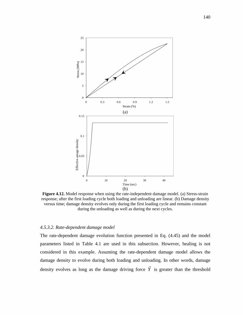
140
(a)
(b)
Figure 4.12. Model response when using the rate-independent damage model. (a) Stress-strain response; after the first loading cycle both loading and unloading are linear. (b) Damage density
versus time; damage density evolves only during the first loading cycle and remains constant during the unloading as well as during the next cycles.
4.5.3.2. Rate-dependent damage model
The rate-dependent damage evolution function presented in Eq. (4.45) and the model
parameters listed in Table 4.1 are used in this subsection. However, healing is not
considered in this example. Assuming the rate-dependent damage model allows the
damage density to evolve during both loading and unloading. In other words, damage
density evolves as long as the damage driving force Y is greater than the threshold
0
0.05
0.1
0.15
0 10 20 30 40
Eff
ectiv
e am
age
dens
ity
Time (sec)
0
5
10
15
20
25
0 0.3 0.6 0.9 1.2 1.5
Str
ess
(MP
a)
Strain (%)

141
damage force thY . However, damage evolves with slower rate during the unloading. The
stress-strain response and evolution of the effective damage density [i.e. 1 h
where 0h since healing is not incorporated] are shown in Figures 4.13(a) and 4.13(b),
respectively. Figure 4.13(a) shows that the model gives a nonlinear response during the
unloading as well as during the loading. This is attributed to the fact that the damage
density can also evolve during the unloading, as shown in Figure 4.13(b).
Figure 4.13. Model responses for the rate-dependent damage model when healing is not considered. (a) Stress-strain response; model predicts nonlinear response during the unloading and loading, hysteresis loops form and energy dissipates at each cycle; (b) Effective damage
density versus time; damage density evolves during both loading and unloading at each cycle; however, the rate of damage evolution decreases as the number of loading cycles increases.
0
0.1
0.2
0.3
0.4
0.5
0.6
0.7
0.8
0.9
0 10 20 30 40
Eff
ectiv
e da
mag
e de
nsity
Time (sec)
0
5
10
15
20
25
0 0.3 0.6 0.9 1.2 1.5
Stre
ss (
MP
a)
Strain (%)
(a)
(b)

142
It should be noted that Ortiz (1985) was the first to model the nonlinear response
of the stress-strain diagram during unloading by considering the anisotropic damage and
crack closure effects. The fundamental assumptions underlying his pioneering work are
schematically illustrated in Figure 4.14.
Figure 4.14. Illustration of the anisotropic damage which has been postulated by Ortiz (1985) to model the nonlinear stress-strain response during the unloading. (a) A schematic RVE with two embedded cracks “A” and “B”; (b) during the loading crack “B” opens and contributes to the degradation of the stiffness; and (c) during the unloading crack “A” opens while partial crack closure occurs at crack “B”. However, the net effect causes the stiffness modulus to degrade
during the unloading.
Figure 4.14(a) shows a schematic RVE with two embedded cracks “A” and “B”
in vertical and horizontal directions, respectively. The RVE presented in Figure 4.14(a)
is subjected to a uniaxial loading-unloading history. During the loading phase [Figure
4.14(b)], crack “B” opens and starts growing which subsequently causes the stiffness
modulus of the material to degrade. However, while crack “B” starts closing and reduces
in size during the unloading phase [Figure 4.14(c)], crack “A” opens and starts growing
as shown in Figure 4.14(c). The reduction in size of crack “B” contributes to the partial
recovery in the stiffness modulus, whereas, the opening of crack “A” during the
unloading contributes to the degradation of the stiffness modulus. Therefore, the change
in the stiffness modulus during the unloading is a competing mechanism between the
effect of the crack closure and crack opening on the stiffness during the unloading.
A B
(a)
AB
(b)
AB
(c)

143
According to the experimental observations, the tangent stiffness modulus usually
decreases gradually during the unloading which is an indication of greater contribution
of the crack opening during the unloading (e.g. Sinha et al., 1964; Karsan and Jirsa,
1969; Ortiz, 1985; Hassan et al., 1992; Eggeler et al., 2004; Sima et al., 2008). In this
work, the anisotropic damage is not considered. However, the nonlinear response during
the unloading is modeled by allowing a time-dependent degradation during the
unloading through a delay-damage (i.e. viscodamage) evolution law. The net
contribution of the closure of crack “A” and opening of crack “B” (Figure 4.14) on the
stiffness reduction during the unloading is captured by allowing the material to gradually
feel the presence of existing cracks during the unloading through crack closure/opening
processes. In other words, at the onset of unloading the material memorizes the damaged
stiffness from the previous loading cycle such that the presence of the newly developed
micro-cracks during the current loading cycle is not felt yet by the material. However,
upon more unloading a gradual opening/closure of existing cracks occurs so that the
material starts gradually feel the presence of those newly developed cracks that will
subsequently cause a gradual stiffness reduction until the complete unloading as
schematically shown in Figure 4.1.
Consequently, one may argue that the commonly observed nonlinear response in
the stress-strain diagram during the unloading could be due to more damage
accumulation. However, careful and extensive experimental measurements should be
conducted before one may prove this argument for a specific type of material. Moreover,
Figure 4.13(a) shows that when damage is allowed to evolve during the unloading,
hysteresis loops form for each loading-unloading cycle. Hence, energy dissipation
continues even after the first loading-unloading cycle which could trigger the fatigue
damage.
The experimental investigations on the cyclic loading of several materials also
show a jump in the tangent stiffness modulus at the unloading-loading points (e.g. point
“A” in the loading history presented in Figure 4.11) (e.g. Sinha et al., 1964; Karsan and
Jirsa, 1969; Ortiz, 1985; Hassan et al., 1992). In other words, the tangent stiffness at the

144
end of the unloading is usually less than the tangent stiffness at the beginning of the next
reloading. However, the rate-dependent damage model is not able to predict this
phenomenon as shown in Figure 4.13(a).
4.5.3.3. Rate-dependent damage and healing model
The rate-dependent damage and healing models presented respectively in Eqs. (4.45) and
(4.48) are used in this section. The damage model parameters are as listed in Table 4.1.
However, the healing model parameters are modified to expedite the healing evolution (
10.8 sh , 1a , 0.001hth ) in order to magnify the healing effect. The stress-strain
response, evolution of the effective damage density [i.e. 1 h ], and the evolution
of the healing variable are shown in Figures 4.15(a), 4.15(b), and 4.15(c), respectively.
Figure 4.15(a) shows the model’s capability in predicting the nonlinear responses during
the unloading. It also shows the formation of hysteresis loops for each loading cycles.
However, interestingly, the model shows the jump in the tangent stiffness at unloading-
loading point (e.g. point “A” in Figure 4.11) when healing is included (this jump can be
seen more clearly in Figure 4.9(b) where the tangent stiffness at the end of unloading is
less than that at the beginning of the reloading when healing is considered). Moreover,
the hysteresis loops converge to a single loop at high loading cycles and tend to stabilize
as shown in Figure 4.15(a) [Figure 4.15(a) shows that the hysteresis loop for loading
cycles 5-7 are very close together and tend to converge to a single loop]. As mentioned
before, the healing condition presented in Eq. (4.49) indicates that the healing variable
starts evolving once the total effective strain is less than the threshold healing strain.
Hence, in the regions close to unloading-loading point (e.g. point “A” in Figure 4.11)
where strain is close to zero, the healing variable increases and subsequently the
effective damage density decreases. Therefore, the material recovers part of its strength
and stiffness at unloading-loading point that causes the stiffness to show a jump at this
point. This observation can also be explained by looking at the effective damage density
variable. As shown in Figure 4.15(b), the effective damage density reaches a plateau as
the number of loading cycle increases. In other words, the newly nucleated micro-

145
damages at large number of loading cycle heals at unloading-loading point, and hence,
the effective damage density reaches a plateau where no more damage accumulation
occurs during the next loading cycle. It also shows that, unlike the commonly postulated
assumptions in CDM, the effective damage density is reversible as a result of micro-
damage healing. Therefore, one may argue that the jump in stiffness at unloading-
loading points might be due to micro-damage healing at low strain levels. Again, careful
experimental tests should be conducted to prove this argument. Figure 4.15(c) shows
that the healing variable decreases during the loading. This decrease can be explained
according to Eq. (4.55). During loading, the area of unhealed damages uhA increases.
Therefore, although the area of the healed damages hA does not change during the
loading, the healing variable decreases since it is defined as the ratio of the healed
damages’ area over the total damaged area (i.e. h Dh A A ).
Figure 4.15. Model response for the rate-dependent damage and healing models. (a) Stress-
strain response; the hysteresis loops tend to converge to a single one as the number of loading cycles increases and model predictions also show the jump in the tangent stiffness modulus at
unloading-loading point. (b) Effective damage density versus time; the effective damage density decreases during the unloading as a result of healing and reaches a plateau at large number of
loading cycles. (c) Healing variable versus time; healing variable increases at small strain levels (close to unloading-loading points), and healing variable decreases during the loading since the
total damaged area increases.
0
5
10
15
20
25
0 0.3 0.6 0.9 1.2 1.5
Stre
ss (
MPa
)
Strain (%)
(a)

146
(b)
(c)
Figure 4.15. Continued.
4.6. Conclusions
A novel continuum damage mechanics-based framework is proposed in this paper to
enhance the continuum damage mechanics theories in modeling the micro-damage
healing phenomenon in materials that tend to self-heal. This framework is proposed by
0
0.1
0.2
0.3
0.4
0.5
0.6
0 10 20 30 40
Eff
ectiv
e da
mag
e de
nsity
Time (sec)
0
0.1
0.2
0.3
0.4
0.5
0.6
0.7
0.8
0 10 20 30 40
Hea
ling
vari
able
Time (sec)

147
extending the concept of the effective configuration and effective stress to the healing
configuration.
Three well-known transformation hypotheses of the continuum damage
mechanics theories (i.e. strain, elastic strain energy, and power equivalence hypotheses)
are also extended for the materials with healing ability. Analytical relations are derived
for each transformation hypothesis to relate the strain tensors, secant stiffness moduli,
and tangent stiffness moduli in the damaged (nominal) and healing configurations.
The presented examples show that the proposed healing framework captures the
recovery in strength and stiffness modulus when healing occurs. The presented example
on the effect of rest periods between loading cycles show that the model predicts more
recovery in the stiffness and strength when the rest time increases such that the material
can recover even all of its strength and stiffness if put in rest for a long enough time.
It is argued that the commonly observed nonlinear responses during the
unloading in the stress-strain response can be modeled using the rate- and time-
dependent damage models. Therefore, it is implied that these nonlinear responses could
be because of more damage accumulation during the unloading.
It is also shown that the jump in the tangent stiffness modulus at unloading-
loading points might be related to micro-damage healing at very small strains. This
framework will be used to model the micro-damage healing in asphaltic materials in the
next chapter. It will be shown that the inclusion of the micro-damage healing
significantly enhances the prediction of the fatigue life in asphalt mixes.
148
CHAPTER V
A MICRO-DAMAGE HEALING MODEL THAT IMPROVES
PREDICTION OF FATIGUE LIFE IN ASPHALT MIXES
5.1. Introduction
As mentioned in Chapters I, II, and IV, various classes of engineering materials
including asphalt binders and asphalt mixes have the potential to heal and retrieve part of
their strength and stiffness with time. In this study, a continuum-based healing model is
proposed in the light of the previous micromechanical and fracture-based models in
order to close the gap in the development of a comprehensive constitutive model for
accurate prediction of the fatigue life of asphaltic materials. The effect of healing is
incorporated into the model by introducing the effective damage density parameter in
which micro-damage healing is considered. This effective damage density is no longer
irreversible. In other words, the effective damage density can decrease during the rest
periods. Consequently, with this effective damage density parameter included, the
continuum model has the capability of capturing changes in material properties such as
strength and stiffness increases during rest period. In addition, a time-dependent
evolution law for the healing parameter is proposed. The proposed evolution law
possesses three model parameters, one of which is directly linked to previous
micromechanical studies (Schapery, 1989; Little and Bhasin, 2007).
The proposed healing model is then coupled to viscoelastic, viscoplastic, and
viscodamage models to enhance that model’s ability to capture the effect of micro-
damage healing and its impact on the mechanical response of asphalt mixes subjected to
repeated loadings in both tension and compression. It is shown that considering the
effect of micro-damage healing significantly enhances the ability of the model to predict
responses under repeated loading during which variable unloading schemes are
introduced. The model predictions show that the fatigue life increases as the rest period
increases (Abu Al-Rub et al., 2010a).

149
5.2. Healing Natural Configuration
In classical CDM, the stresses in a fictitious undamaged (but not healed) configuration
are related to the stresses in the nominal (damaged) configuration as follows:
1
ijij
(5.1)
where is the undamaged stress tensor, is the damaged (nominal) stress tensor, and
is the so-called damage variable or damage density. The damage process is primarily
assumed to be irreversible in continuum damage mechanics. Hence, an increasing
function with time is usually postulated for describing the damage variable
(Kachanov, 1958, 1986; Lemaître, 1992; Kattan and Voyiadjis, 1993; Krajcinovic, 1996;
Abu Al-Rub and Voyiadjis, 2005b).
However, as discussed in Chapter IV, some engineering materials and
specifically asphalt mixtures have the potential to heal and recover part of their strength
and stiffness under specific conditions such as resting periods during repeated or fatigue
loading. Hence, a proper CDM framework should be developed in order to describe the
changes in the material’s microstructure during the healing process (see Figure 5.1).
Figure 5.1. Extension of the effective stress concept in continuum damage mechanics to damaged-healed materials.
Fictitious healing configuration
Damaged-unhealed configuration
Damaged-partially-healedconfiguration
Remove unhealed micro-voids and
micro-cracks Rest period

150
Therefore, the micro-damage healing framework proposed in Chapter IV is adopted to
define a natural configuration named the healing configuration as shown in Figure 5.1.
In this natural configuration, one can simply define an effective damage density,
, that considers the density of healed micro-cracks and micro-voids as follows:
1 h (5.2)
where h is referred to in this paper as the micro-damage healing internal state variable
since it defines the density of healed micro-cracks and micro-voids. Using the definition
proposed in Eq. (5.2), one can replace the definition of the effective stress in Eq. (5.1) by
another effective stress that considers micro-damage healing, such that:
1 11
ij ijij h
(5.3)
where is the stress tensor in the healing configuration as demonstrated in Figure 5.1.
In the above and subsequence, the superimposed “ ” designates the healing
configuration of the material. Note that when 0h (i.e. ), Eqs. (5.1) and (5.3) are
identical which implies that no healing has occurred in the material. On the other hand,
when 1h (i.e. 0 ), the nominal stress tensor and the effective stress tensor in the
healing configuration are the same, which implies that all micro-damage has healed;
and hence, the material has completely recovered its strength and stiffness. Moreover,
one notice that when the material is initially undamaged, 0h and .
It is assumed here that once a material is damaged, further loading only affects
the portion of the material that is intact and partially or completely healed. In other
words, further loading is carried out by the material in the healing configuration shown
in Figure 5.1. Hence, in the subsequent developments, the constitutive equations are
expressed in the healing configuration.

151
5.3. Constitutive Model
5.3.1. Thermo-Viscoelastic-Viscoplastic-Viscodamage Model
The viscoelastic-viscoplastic-viscodamage constitutive model remains the same
as presented in Chapter II with the difference that they should be represented in the
healing configuration instead of the effective (undamaged) configuration. In other words
one can simply replace the superimposed “ ” by “ ” in order to represent the thermo-
viscoelastic-viscoplastic-viscodamage model in the undamaged-healed configuration
(please refer to Chapter II for a complete detail on the constitutive model). Therefore, in
order to avoid the repetition, the thermo-viscoelastic-viscoplastic-viscodamage
constitutive model is not presented in this chapter.
5.3.2. Proposed Micro-Damage Healing Model
Wool and O’connor (1981) proposed a phenomenological-based theory for the crack
healing in polymers. They defined a macroscopic recovery parameter that relates the
healing at the micro-scale to the changes in the mechanical properties of polymers at the
macro scale. They introduced the macroscopic recovery parameter as the ratio of the
mechanical properties of the material such as the fracture stress, the failure strain, the
tensile modulus, and the fracture energy subjected to a healing history over the
corresponding mechanical properties of the material in the original state (Wool and
Oconnor, 1981). They defined through the following convolution integral:
,t
I
d Xt d
d
(5.4)
where I t is an intrinsic healing function that incorporates wetting (i.e. the free
surfaces of a crack get closer and touch each other) and diffusion (i.e. inter-molecular
flow of matter) and defines the rate at which the two wetted surfaces heal and recover
part of their original strength. Therefore, the intrinsic healing function is additively
decomposed into an intrinsic healing due to short-term wetting 0I , which is controlled
by the surface energy, and the intrinsic healing due to long-term diffusion, dI .
152
Moreover, ,X t in Eq. (5.4) is defined as the wetting distribution function. Wool and
O'connor (1981) also investigated two cases for ,X t ; instantaneous wetting and
constant rate wetting. In the case of instantaneous wetting, the two crack surfaces touch
each other immediately which implies:
,t X t (5.5)
where t is the Dirac-delta function. As a result, the macroscopic recovery parameter
in Eq. (5.4) and the intrinsic healing function become identical, such that:
0 dI I It t (5.6)
However, for a constant rate of wetting one can write:
, wt X k U t (5.7)
where wk is the wetting rate and U t is the Heaviside step function (i.e. 1U for
0t and 0U for 0t ). In this case, the macroscopic recovery parameter can be
expressed as:
0 dw Ik t t (5.8)
where d t is the component of the macroscopic recovery parameter due to diffusion.
Power or exponential expressions can be assumed for d such that 21
cd c t or
1 2[1 exp( )]d c c t , respectively, where 1c and 2c are material parameters.
Comparing Eqs. (5.6) and (5.8) reveals that the wetting component of the macroscopic
recovery parameter is time-independent in case of instant wetting and time-dependent
for the case of constant wetting rate. Using Eq. (5.6), Eq. (5.8), or another expression
depends on how experimental data shows the variation of with the healing time.
Therefore, it is obvious that Eqs. (5.6) or (5.8) are fitting functions that can be
empirically assumed with a large number of material constants without explicit
consideration of the driving forces for healing.
On the other hand, Schapery (1989) has developed a model for rate of crack size
reduction ba in linear, isotropic, viscoelastic materials based on fracture mechanics. He

153
related ba to fundamental material properties such as the size of the fracture processed
zone, , the surface energy, , the interface bond strength, b , the Poisson’s ratio ,
and the viscoelastic material properties. It is noteworthy to mention that in the
Schapery’s formulation (1989) the whole healing process is considered. In other words,
he did not distinguish between the healing due to wetting and the healing due to
diffusion since he assumed that the healed part of a crack retrieves its total original
strength.
Little and Bhasin (2007) and Bhasin et al. (2008) used the work of Wool and
O’connor (1981) and Schapery (1989) and utilized the macroscopic recovery parameter
R in Eq. (5.4) to describe the effect of healing in bituminous materials. They used a
simplified form of the crack shortening rate (Schapery, 1989) as the rate of the wetting
function, such that:
1
02 21
, 1
4(1 )
mc
bm b
d t X Wa D
dt D k
(5.9)
where 0D , 1D , and m are obtained by assuming a power law function for the transient
creep compliance in Eq. (2.9) (i.e. 1mD D t ), and mk is a material constant expressed
in terms of m . Moreover, 2cW G is the work of cohesion and is related to the
material’s surface energy G . In obtaining Eq. (5.9), Schapery (1989) assumed that the
bond strength, b , along in the healing process zone, , is constant. Therefore, one
concludes that the rate of wetting function in Eq. (5.9) utilized by Little and Bhasin
(2007) and Bhasin et al. (2008) is constant. This reduces the healing convolution integral
in Eq. (5.4) to the form in Eq. (5.8) such that w bk a . Also, Little and Bhasin (2007)
have assumed a three-parameter expression for d in Eq. (5.8) such that
31 2[1 exp( )]cd c c t . Therefore, identifying these parameters ( 1c , 2c , 3c ) in addition
to those in Eq. (5.9) for an asphalt mixture is a challenge. Moreover, based on limited
experimental data, they showed that healing in asphalt binders follow Eq. (5.6) and not

154
Eq. (5.8), which implies that instantaneous healing occurs upon the wetting of cracks
free surfaces.
However, one realizes that the aforementioned healing models are mostly
fracture mechanics-based and micromechanically-based and cannot be used easily at the
scale of the asphalt mixture. These models are also augmented with many material
parameters that are difficult to identify experimentally. Furthermore, their coupling to
the viscoelastic, viscoplastic, and rate- and time-dependent damage response of materials
is not clear. On the other hand, one need an evolution law for the micro-damage healing
internal state variable in Eq. (5.3) to establish this coupling and incorporates healing into
the current constitutive equations. According to the aforementioned healing models and
intuitively, one expects that the proposed healing variable h should be a function of
resting period (or healing time), temperature, level of damage, and the history of healing.
Hence, one can incorporate all these effects into the following postulated
phenomenological-based healing evolution equation:
1 21 1b bhh T h (5.10)
where h dh dt is the rate of the healing variable, h T is the healing viscosity
parameter that determines how fast the material heals which is a function of temperature
T ; and 1b and 2b are material constants. Moreover, the following expression can be
assumed for h T :
0 30
exp 1h h TT
T
(5.11)
where 0h is the healing viscosity parameter at reference temperature 0T , and 3 is the
healing temperature coupling model parameter. Eqs. (5.10) and (5.11) state that the
healing rate increases as the temperature exceeds the reference temperature and
decreases for temperatures less than the reference temperature. Also, the parameter 0h
has the unit of Sec-1 and determines how fast the material heals. One can argue that 0h
increases as the surface energy increases and shows that a material with larger surface

155
energy heals faster than a material with smaller surface energy. Note that at reference
temperature and when 1 2 0b b , Eq. (5.10) simplifies as follows:
0hh (5.12)
which states that the rate of healing is constant. This is the simplest evolution equation
one can assume for the healing variable h . In fact, this is the case in Eq. (5.9)that is
derived by Schapery (1989) based on the assumption of a constant bond strength, b ,
along the healing process zone, . Therefore, by assuming /bh a , one may relate
0h to more fundamental material properties by comparing Eqs. (5.9) and (5.12), such
that:
1
0 02 21
1 2
4(1 )
mh
m b
GD
D k
(5.13)
Eq. (5.13) bridges the gap between the model developed at the micro-scale, Eq. (5.9),
and the proposed model at the macro-scale, Eq. (5.10).
It is noteworthy that, for the general case (i.e. 1 0b and 2 0b ) in Eq. (5.10),
the healing viscosity parameter can be considered as the maximum rate at which the
healing occurs. In other words, the healing rate decreases either when the healing
variable increases [controlled by (1 h ) term] or when the density of micro-cracks
increases [controlled by (1 ) term]. These arguments are in agreement with those by
Schapery (1989) and the experimental observations by Little and Bhasin (2007) and
Bhasin et al. (2008).
Moreover, one can obtain the evolution expression in Eq. (5.10) based on the
laws of thermodynamics through assuming h to be an internal state variable in the
Helmholtz free energy . Thus, the corresponding thermodynamic conjugate force, H ,
can be interpreted as the strain energy recovery rate, such that
Hh
(5.14)

156
where h cH with c being a material property. Thus, using Eqs. (5.10) and (5.14), one
can obtain an expression for and H that yields the evolution equation for the healing
variable h . Details of this thermodynamic approach are presented by Darabi et al.
(2011d).
5.4. Finite Element Implementation
The finite element implementation of the thermo-viscoelastic-viscoplastic component of
the constitutive model remains the same as explained in Chapter II. However, as
mentioned before, the viscoelastic and viscoplastic models are presented in the healing
configuration. The viscodamage and micro-damage healing models are incorporated into
the model using the concept of the undamaged-healed stress space.
Hence, once the updated stress in the healing configuration, then calculate the
rate of the damage density and the rate of healing variable using Eqs. (2.45) and (5.10)
such that the total damage density and healing variables can then be obtained as follows:
t t t t t (5.15)
t t t th h h t (5.16)
Finally, the nominal stress tensor can be updated using Eq. (5.3) [refer to Chapter IV for
a detailed description of implementation procedure of the healing and damage models].
To clarify the implementation steps, a flowchart showing the implementation process in
a straightforward manner is presented in Figure 5.2.
The formulated numerical algorithms presented in this section are implemented
in the well-known finite element code Abaqus (2008) via the user material subroutine
UMAT.

157
Figure 5.2. Flowchart for numerical implementation of the proposed coupled thermo-viscoelastic-viscoplastic-viscodamage-healing constitutive model.
Calculate the residual strain Eq. (2.65).
Input history variables and the total strain increment
Recalculate the stress-dependent parameters based on the current trial stress
Approximate viscoelastic stress-dependent parameters using the previous converged stress and calculate the trial stresses using Eqs. (2.53) and (2.54).
Calculate the tangent stiffness [Eq. (2.67)] and stress correction [Eq. (2.66)]
Calculate the viscoelastic strain increments from Eqs. (2.49) and (2.50).
Put viscoplastic strain increment=0
Calculate viscoplastic strain increment based on the current trial stress by using the local Newton-Raphson method [Eq. (2.64)].
Correct trial stress Eq. (2.66).
tijR Tolerance
Update the effective stress and history variables using Eqs. (2.46)-(2.48)
Calculate the rate of damage evolution and the damage density using Eqs. (2.45) and (5.15).
Calculate the rate of healing variable, Eq. (5.11), healing variable, Eq. (5.16), and the effective damage density, Eq. (5.2).
Update the stress in the nominal configuration, Eq. (5.3), tangent compliance, Eq. (2.67), and history variables and pass them as the updated variables
No Yes
No No
Yes Yes
1 0vpf I

158
5.5. Application of the Model for Prediction of Response of Asphalt Mixes
5.5.1. Identification of the Micro-Damage Healing Model Parameters
It was shown in Chapter II that the coupled thermo-viscoelastic-viscoplastic-
viscodamage model fails to predict reasonable behavior for the repeated creep-recovery
tests with the introduced rest period. In this chapter, the proposed micro-damage healing
model is coupled to the rest of the constitutive model to enhance the model in predicting
the fatigue behavior of asphalt mixes. The identified thermo-viscoelastic-viscoplastic-
viscodamage model parameters for the Dense Bitumen Macadam mixture discussed in
Chapter II listed in Table 2.2 and 2.3.
The identified viscoelastic, viscoplastic, and viscodamage model parameters can
now be used for prediction of repeated creep-recovery tests. However, the model without
the healing component predicts shorter fatigue life comparing to experimental
measurements, as discussed earlier. In other words, the model predicts higher creep
strains comparing to experimental data. This effect is due to the fact that the damage
density in the viscodamage model is considered to be irreversible, and hence, does not
allow for damage recovery or healing during the rest period. This effect will be more
pronounced for long rest periods. Hence, one can conclude that the difference between
the experimental measurements and model predictions of creep strain should be
compensated with the healing model. Hence, one can determine the healing viscosity
parameter 0h at reference temperature and the history parameters 1b and 2b by adjusting
the model predictions to be comparable with the experimental measurements. In this
study, the repeated creep-recovery test in compression when loading time is 60 sec and
unloading time is 100 sec is selected for determination of healing model parameters. The
identified healing model parameters in Eq. (5.11) are 3 10 2.5 10 Sech , 1 3b , and
2 6b . The flowchart for describing the procedure for calibrating the model in the
presence of the micro-damage healing is updated and presented in Figure 5.3.

159
Figure 5.3. The procedure for identification of the coupled thermo-viscoelastic-viscoplastic-viscodamage-healing constitutive model parameters.
5.5.2. Prediction of Fatigue Life in Asphalt Mixes
Recently, Gibson et al. (2009) have simulated several pavement structures with eight
inch asphalt layer subjected to dual tires with both 80 kN and 178 kN single axle loads.
They calculated the first stress invariant 1I and the second deviatoric stress invariant
Get healing model parameters 0h , 1b , and 2b using a repeated creep-recovery test in
compression [Eq.(5.11)].
Separate viscoelastic response in the recovery part of the creep-recovery tests using Eq. (2.76).
Identify the Prony series coefficients nD and n at the reference temperature using
Eqs. (2.9) and (2.76).
Calculate 1vp , 2
vp , and p from the creep part of the creep-recovery tests using Eqs.
(2.80), (2.81), and (2.82).
Identify the viscoplastic model parameters at the reference temperature by minimizing the error between the experimental measurements and Eq. (2.79).
Identify vd and k from a creep test at the reference temperature and stress level using Eq. (2.85).
Identify viscodamage stress dependency parameter q from a creep test at the
reference temperature, when ref using Eq. (2.84).
Identify temperature coupling terms model parameters by comparing experimental data and model predictions at different temperatures using Eqs. (2.90) and (2.91).
Identify vpd and vpd from two creep tests in tension using Eqs. (2.23) and. (2.44).

160
2J at different positions under the dual tire configuration. These multiaxial states of
stresses relatively represent the actual state of stress in asphalt pavements subjected to
wheel loads.
In this work, the applied stress level for the repeated creep-recovery test in
compression is assumed to be 1500 kPa whereas the applied stress level for the repeated
creep-recovery test in tension is assumed to be 300 kPa. These two stress levels are close
to the maximum compressive and tensile stress levels in the asphalt layer analyzed by
Gibson et al. (2009).These tests are conducted at temperature of 20oC.
Figures 5.4(a), 5.5(a), and 5.6(a) show the experimental results and model
predictions for repeated creep-recovery tests in compression where the applied stress
level is 1500 kPa. Figure 5.4(a) shows the creep strain versus time when the loading time
is 120 sec and the unloading time is 100 sec. As it is shown in Figure 5.4(a), the model
predictions when healing is included are significantly improved as compared to the
experimental data and the predictions when healing is not included. The evolution of the
effective damage density (i.e. without healing and 1 h with healing) is
shown in Figure 5.4(b). As shown in Figure 5.4(b), for model predictions where healing
is not considered, the effective damage density increases rapidly during loading and
remains constant during unloading, whereas the model predictions when healing is
included show that the effective damage density decreases during the resting periods. In
other words, by including the healing parameter the effective damage density is no
longer irreversible and can decrease during the resting time. Moreover, the model
predictions without healing and damage significantly underestimate the total creep
strain. It is noteworthy that failure in the simulated repeated creep-recovery test in, for
example, Figure 5.4(a) is defined by the onset that the compliance reaches a very large
value close to infinity or when the stiffness modulus reaches a very small value close to
zero. One notice from Figure 5.4(b) that the damage density increases with increasing
loading cycles such that at some loading cycles the creep response in Figure 5.4(a)
reaches the tertiary stage with an exponential increase in the total creep strain during the
loading cycles.

161
(a)
(b)
Figure 5.4. Repeated creep-recovery test in compression with 120sec loading time and 100sec resting period. (a) Compared creep strain, and (b) the evolution of the effective damage density.
The end of the cyclic tertiary stage indicates the failure is similar to a standard
creep test. Figure 5.5 shows the results when the loading time is 60 sec and the resting
period is 100 sec.
0
1
2
3
4
5
6
7
8
9
0 200 400 600 800 1000
Axi
al st
rain
(%
)
Time (Sec)
Experimental data
Model prediction without healing
Model prediction including healing
Model prediction without healing and damage
0.0
0.1
0.2
0.3
0.4
0.5
0.6
0.7
0.8
0 200 400 600 800 1000
Eff
ecti
ve d
amag
e de
nsit
y
Time (Sec)
Model prediction without healing
Model prediction including healing

162
(a)
(b)
Figure 5.5. Repeated creep-recovery test in compression with 60sec loading time and 100sec resting period. (a) Total experimental creep strain, and model predictions of total creep strain
with and without damage and healing components, (b) model predictions for viscoelastic strain with and without damage and healing components, (c) model predictions for viscoplastic strain
with and without damage and healing components, and (d) the evolution of the effective damage density.
0
1
2
3
4
5
6
7
8
9
10
0 500 1000 1500 2000
Axi
al st
rain
(%
)
Time (Sec)
Experimental data
Model prediction without healing
Model prediction with healing
Model prediction without healing and damage
0.0
0.2
0.4
0.6
0.8
1.0
1.2
1.4
1.6
0 500 1000 1500 2000
Axi
al v
isco
elas
tic
stra
in (
%)
Time (Sec)
Model prediction without healing and damage
Model prediction without healing
Model prediction with healing

163
(c)
(d)
Figure 5.5. Continued.
Figure 5.5(a) shows that the model without healing predicts failure after only 6
cycles; whereas, the model without damage and healing significantly underestimates the
creep strain and also is not able to predict failure. However, experimental measurements
and model predictions when healing is considered are in good agreement and show that
the material can sustain more loading cycles. In order to study the effects of damage and
0
1
2
3
4
5
6
7
8
0 500 1000 1500 2000
Axi
al v
isco
plas
tic
stra
in (%
)
Time (Sec)
Model prediction without healing and damage
Model prediction without healing
Model prediction with healing
0.0
0.1
0.2
0.3
0.4
0.5
0.6
0 500 1000 1500 2000
Eff
ecti
ve d
amag
e de
nsit
y
Time (Sec)
Model prediction without healing
Model prediction including healing

164
healing on viscoelastic and viscoplastic deformations, the model predictions for
viscoelastic and viscoplastic strains with and without damage and healing are presented
in Figures 5.5(b) and 5.5(c), respectively. Figures 5.5(b) and 5.5(c) show that the
proposed model predicts larger values for both the viscoelastic and viscoplastic strains
when damage and healing are activated. However, the increase in the viscoplastic strain
is much larger than that in the viscoelastic strain. Moreover, Figure 5.5(d) shows that the
damage density reaches a large value after few cycles when not considering healing;
whereas, the effective damage density evolves at a much slower rate when the healing is
included.
The effect of healing becomes more pronounced when the total duration of
resting period increases. Interesting results are shown in Figure 5.6 when the loading
duration is 60 sec and the resting time is 1500 sec. The long resting period provides
enough time for significant healing to take place. The model predictions without
considering healing show that the material fails after 6 cycles as shown in Figure 5.6(a).
However, experimental results demonstrate that the material can tolerate loading for
many more loading cycles.
As shown in Figure 5.6(a), the model that considers healing is able of capturing
this behavior and is also able to predict the experimental measurements fairly well.
Figure 5.6(a) also shows that the model predictions without healing and damage
significantly underestimate the total creep strain. Again, as shown in Figure 5.6(b), the
effective damage density when healing is not included grows rapidly; whereas, the
inclusion of healing reduces the amount of damage and extends the fatigue life the
asphalt mix.

165
(a)
(b)
Figure 5.6. Repeated creep-recovery test in compression with 60sec loading time and 1500sec resting period. (a) Compared creep strain, and (b) the evolution of the effective damage density.
The repeated creep-recovery test is also performed in tension as well and used to
validate the healing model. Tensile creep-recovery tests Figures 5.7(a)-5.10(a)) are
conducted at room temperature where the applied stress is 300kPa. Two different
loading times of 120 sec and 60 sec are considered. Figure 5.7 shows the model
0
2
4
6
8
10
12
14
0 10000 20000 30000 40000
Axi
al st
rain
(%
)
Time (Sec)
Experimental data
Model prediction without healing
Model prediction including healing
Model prediction without healing and damage

166
predictions with and without consideration of the healing compared to experimental
measurements with 120 sec loading time and 100 sec resting period.
(a)
(b)
Figure 5.7. Repeated creep-recovery test in tension with 120sec loading time and 100sec resting period. (a) Compared creep strain, and (b) the evolution of the effective damage density.
0
1
2
3
4
5
0 200 400 600 800 1000 1200
Axi
al st
rain
(%
)
Time (Sec)
Experimental data
Model prediction without healing
Model prediction including healing
Model prediction without healing and damage
0.0
0.1
0.2
0.3
0.4
0.5
0.6
0.7
0 200 400 600 800 1000 1200
Eff
ecti
ve d
amag
e de
nsit
y
Time (Sec)
Model prediction without healing
Model prediction including healing

167
Obviously, since damage is more severe in tension than in compression, the
model predictions of the repeated creep-recovery response without considering healing
significantly overestimates the amount of creep strain and damage evolution. Therefore,
it is essential to incorporate healing into the fatigue damage predictions especially under
tensile fatigue loading conditions. The evolution of the effective damage density is also
shown in Figure 5.7(b). Moreover, experimental measurements and model predictions
with and without healing for a loading time duration of 60 sec and for three different
unloading times (50, 100, and 1500 sec) are compared in Figures 5.8, 5.9, and 5.10,
respectively.
The model predictions when the healing parameter is considered significantly
improve the prediction of experimental data. The calculated effective damage density
when the loading duration is 60 sec and the unloading durations are 50, 100, and 1500
sec are plotted in Figures 5.8(b), 5.9(b), and 5.10(b), respectively. These figures show
that when the micro-damage healing is considered the damage density decreases during
the rest period due to the micro-damage healing. Also, one can clearly notice from
Figure 5.10(b) that the damage density per loading cycle decreases as the number of
cycles increases.

168
(a)
(b)
Figure 5.8. Repeated creep-recovery test in tension with 60sec loading time and 50sec resting period. (a) Compared creep strain, and (b) the evolution of the effective damage density.
0.0
0.5
1.0
1.5
2.0
0 200 400 600 800 1000
Axi
al st
rain
(%
)
Time (Sec)
Experimental data
Model prediction without healing
Model prediction including healing
Model prediction without healing and damage
0.0
0.1
0.2
0.3
0.4
0.5
0 200 400 600 800 1000
Eff
ecti
ve d
amag
e de
nsit
y
Time (Sec)
Model prediction without healing
Model prediction including healing

169
(a)
(b)
Figure 5.9. Repeated creep-recovery test in tension with 60sec loading time and 100sec resting period. (a) Compared creep strain, and (b) the evolution of the effective damage density.
0.0
0.5
1.0
1.5
2.0
2.5
3.0
0 500 1000 1500 2000
Axi
al st
rain
(%
)
Time (Sec)
Experimental data
Model prediction without healing
Model prediction including healing
Model prediction without healing and damage
0.0
0.1
0.2
0.3
0.4
0.5
0 500 1000 1500 2000
Eff
ecti
ve d
amag
e de
nsit
y
Time (Sec)
Model prediction without healing
Model prediction including healing

170
(a)
(b)
Figure 5.10. Repeated creep-recovery test in tension with 60sec loading time and 1500sec resting period. (a) Compared creep strain, and (b) the evolution of the effective damage density.
These reported results clearly show that considering the effect of the micro-
damage healing significantly improves the ability of the current viscoelastic,
viscoplastic, and viscodamage constitutive model in predicting the fatigue life of asphalt
mixtures in the presence of rest periods. Whereas, neglecting micro-damage healing
0.0
0.5
1.0
1.5
2.0
2.5
3.0
3.5
0 5000 10000 15000 20000 25000
Axi
al st
rain
(%
)
Time (Sec)
Experimental data
Model prediction without healing
Model prediction including healing
Model prediction without damage and healing
0.0
0.1
0.2
0.3
0.4
0.5
0 5000 10000 15000 20000 25000
Eff
ecti
ve d
amag
e de
nsit
y
Time (Sec)
Model prediction without healing
Model prediction including healing

171
makes such a complex constitutive model significantly underestimates the fatigue life,
and in turn to very conservative designs of our asphalt pavements. However, more
experimental data for different loading conditions, especially at different temperatures, is
needed for validating and improving the predictions of the proposed healing model.
It is noteworthy that for healing to impact the damage process, micro-crack
development must occur. The damage that is recorded during the currently utilized
repeated creep and recovery tests is consistent with the development of micro-cracks.
This is because the experiments are performed at 20oC and the periods of loading under
large stress levels are sufficiently long to cause micro-crack development and growth.
Therefore, although these cyclic creep and recovery experiments do not represent what
might be considered as “classical” fatigue experiments to most pavement engineers
where thousands of loading cycles at low stress or strain levels are applied to cause
failure, it does indeed represent the type of damage and recovery in asphalt pavements
that leads to fatigue failure.
5.6. Effect of Healing Model Parameters
In this section, the effect of healing model parameters on damage performance of
asphalt mixes is investigated. For this purpose, the repeated creep-recovery test
subjected to 1500 kPa compressive load when loading time is 60 sec and unloading time
is 100 sec is re-simulated using different values for the healing model parameters 0h , 1b
, and 2b . Figure 5.11 shows the effect of healing viscosity parameter, 0h , on the fatigue
life prediction. The values of history parameters are set to be zero (i.e. 1 2 0b b ) in
this figure. As is shown in Figure 5.11(a) the fatigue life increases as 0h increases due
to the increased levels of micro-crack healing. Therefore, 0h controls the rate at which
healing occurs such that one can classify different materials for their potential to heal
based on the value of this parameter. Figure 5.11(b) shows the corresponding evolution
of the effective damage density, . This figure shows that for very large values of 0h
the effective damage density approaches zero indicating that the accumulated resting

172
period is sufficient for complete healing of existing micro-cracks. However, as the
healing viscosity parameter decreases, the decrease in the effective damage density
during the rest period slows down, and hence, the model predicts shorter fatigue lives.
The effects of the history parameters 1b and 2b are shown in Figures 5.12 and 5.13,
respectively.
(a)
(b)
Figure 5.11. Effect of healing viscosity parameter 0h on fatigue behavior of asphalt mixes. (a)
total strain versus time and (b) effective damage density versus time.
0.0
0.1
0.2
0.3
0.4
0.5
0.6
0 300 600 900 1200 1500 1800
Eff
ecti
ve d
amag
e de
nsit
y
Time (Sec)
32.5 10 / sec
47.5 10 / sec
45.0 10 / sec
42.5 10 / sec
No healing
0
1
2
3
4
5
6
7
8
9
0 300 600 900 1200 1500 1800
Axi
al st
rain
(%
)
Time (Sec)
32.5 10 / sec
47.5 10 / sec
45.0 10 / sec42.5 10 / sec
No healing

173
Figure 5.12 shows the effect of damage history parameter 1b when 30 10 / sech and
2 0b . Figures 5.12(a) and 5.12(b) show that the material’s potential to heal increases as
1b decreases. Therefore, the healing rate decreases as the damage density increases. In
other words, it becomes more difficult to heal the crack as it grows bigger and bigger.
(a)
(b)
Figure 5.12. Effect of damage history parameter 1b on fatigue behavior of asphalt mixes when 3
0 1.0 10 / sech and 2 0b . (a) total strain versus time and (b) effective damage density versus time.
0.00
0.05
0.10
0.15
0.20
0.25
0.30
0.35
0.40
0 500 1000 1500 2000 2500 3000
Eff
ecti
ve d
amag
e de
nsit
y
Time (Sec)
1 0b
1 10b 1 5b
1 2b
1 0b
1 2b
1 5b
1 10b
0
2
4
6
8
10
12
0 500 1000 1500 2000 2500 3000
Axi
al st
rain
(%
)
Time (Sec)

174
The effect of the healing history parameter 2b on the total strain and effective
damage density is presented in Figures 5.13(a) and 5.13(b), respectively. Figures 5.13(a)
and 5.13(b) show trends similar to that in Figure 5.12(a) and Figure 5.12(b),
respectively. This is in qualitative agreement with the experimental results by Little and
Bhasin (2007) who showed that the rate of healing approaches zero upon complete
healing of micro-cracks. Therefore, results for negative values for 2b are not shown here.
However, more experimental studies are needed to verify and validate the
aforementioned qualitative predictions of the proposed micro-damage healing model.
5.7. Conclusions
In this chapter, a micro-damage healing model is proposed based on extending the
effective stress concept in classical continuum damage mechanics by introducing a
fictitious effective undamaged-healed natural configuration. The proposed micro-
damage healing model is coupled with temperature-dependent nonlinear viscoelastic,
viscoplastic, and viscodamage constitutive models that can predict the highly nonlinear
mechanical responses of asphalt mixtures subjected to repeated loading conditions.
Moreover, motivated by previously developed micromechanical- and fracture-
based healing models, a phenomenological healing equation is proposed for the
evolution of the micro-damage healing internal state variable. The healing evolution
equation is time, temperature, and loading/unloading history dependent model that
explicitly affect the stress state and the viscoelastic, viscoplastic, and viscodamage
response of the material while undergoing micro-damage healing. Moreover, an attempt
is made to relate the material parameter that controls the rate of healing to the surface
energy and bond strength of the material. Finally, the model is calibrated and validated
against repeated creep-recovery experimental data on an asphalt mixture with different
loading and unloading times and under tensile compressive stress states.

175
(a)
(b)
Figure 5.13. Effect of healing history parameter 2b on fatigue behavior of asphalt mixes when 3
0 1.0 10 / sech and 1 0b . (a) total strain versus time and (b) effective damage density versus time.
It is shown that for the accurate prediction of the fatigue life of asphalt mixtures
subjected to repeated loading-unloading conditions, a robust micro-damage healing
model should be incorporated into the constitutive behavior of materials. Neglecting the
0.00
0.05
0.10
0.15
0.20
0.25
0.30
0.35
0.40
0.45
0 500 1000 1500 2000 2500 3000
Eff
ecti
ve d
amag
e de
nsit
y
Time (Sec)
2 0b
2 2b
2 5b 2 10b
0
2
4
6
8
10
12
0 500 1000 1500 2000 2500 3000
Axi
al st
rain
(%
)
Time (Sec)
2 0b
2 2b 2 5b
2 10b

176
micro-damage healing phenomenon leads to significant deviations between the
constitutive model predictions and the fatigue life of materials that have potential to
heal. In fact, very conservative designs are made if such models are used in guiding the
design of structural systems made of such material.
The model predictions when micro-damage healing is considered show that the
effective damage density decreases during the rest period; and thus, fatigue life
increases. It is shown that for long unloading or resting periods the effective damage
density (i.e. density of the unhealed micro-cracks and micro-voids) increases at a very
low rate as the number of loading cycle increases. Hence, the proposed micro-damage
healing model can be used effectively to predict the pavement performance during the
service life since pavements are, at least intermittently, subjected to repeated loading
conditions with relatively long rest periods compared to the duration of loading periods.
The present analysis considers repeated creep-recovery tests with different
loading and unloading times in both tension and compression at room temperature.
However, more tests are needed to fully validate the model, especially at different
temperatures. Furthermore, the inclusion of environmental factors such as moisture and
aging is necessary since the ultimate goal is to predict the response of the asphalt
pavements during their service life.
Moreover, the proposed constitutive model is used specifically for asphalt mixes.
However, a wide range of materials show time-, temperature-, and rate-dependent
viscoelastic, viscoplastic, viscodamage, and healing responses. Therefore, it is
imperative to develop a general and robust thermodynamic framework with the
capability to derive new constitutive models for different materials or to enhance the
existing ones without violating the very fundamental laws of thermodynamic. This
investigation will be the subject of the next chapter.

177
CHAPTER VI
A NEW GENERAL THERMODYNAMIC-BASED FRAMEWORK
FOR CONSTITUTIVE MODELING OF TIME- AND RATE-
DEPENDENT MATERIALS
6.1. Introduction
As mentioned in the previous chapters, accurate prediction of mechanical response of
time- and rate-dependent materials requires the coupling between temperature-dependent
viscoelasticity, viscoplasticity, viscodamage, and healing models. These models, on the
other hand, should be general such that they can be applied for a wide range of loading
conditions and the complex three dimensional stress states. One of the approaches is to
derive the models from the fundamental laws of mechanics such that they do not violate
the fundamental laws of thermodynamics. This approach makes the model more
consistent and reliable.
However, even derivation of the models based on the fundamental laws of the
thermodynamics is usually associated with certain assumptions. These assumptions may
reduce the reliability of the derived constitutive models. Therefore, this chapter is
devoted to development of a general thermodynamic-based framework which can be
used to derive different constitutive models for the time- and rate-dependent materials
with the least possible assumptions. This framework is general and can be used for
derivation of constitutive models for a wide variety of materials including bituminous
materials, polymers, bio-inspired materials, and soft materials.
Numerous thermodynamic-based models have been proposed in the literature to
couple one or two of the mechanisms such as viscoelastic, viscoplastic, and/or
viscodamage to describe the behavior of different materials such as metals, polymers,
soft materials, and bio-inspired materials (e.g. Kachanov, 1986; Voyiadjis and Kattan,
1990; Lemaître, 1992; Schapery, 1999; Voyiadjis and Park, 1999; Rajagopal and
Srinivasa, 2000; Tao et al., 2001; Abu Al-Rub and Voyiadjis, 2003; Boubakar et al.,
2003; Barot et al., 2008; Ghorbel, 2008; Levesque et al., 2008; Karra and Rajagopal,

178
2009). However, depending on the loading conditions, many types of time- and rate-
dependent materials show all four mechanisms under thermo-mechanical loading which
makes it necessary to develop a general framework for coupling all four mentioned
mechanisms.
Schapery (1969a) derived a single integral equation using the thermodynamics of
irreversible processes for constitutive modeling of non-linear viscoelastic materials such
as polymers. Several authors have extended the 1D Schapery’s constitutive theory to the
3D viscoelastic models directly from the one-dimensional model presented by Schapery
(Henriksen, 1984; Touati and Cederbaum, 1998; Beijer and Spoormaker, 2002; Haj-Ali
and Muliana, 2004; Levesque et al., 2004). Recently, Levesque et al. (2008) showed
that these 3D applications were thermodynamically inconsistent extensions of the 1D
Schapery’s viscoelastic model, and formulated a thermodynamically consistent 3D
Schapery-type viscoelastic model. However, they considered the Cauchy stress tensor as
the thermodynamic conjugate force of the total viscoelastic strain tensor. This
assumption is valid only for a reversible load history for which the state variables
associated with viscoelastic process remain constant and, hence, is not general.
In terms of the viscoplastic behavior of rate-dependent materials, Perzyna’s
viscoplastic model (Perzyna, 1971) has been used by several researchers to predict the
permanent deformation in these materials (e.g. Masad et al., 2005; Saadeh et al., 2007;
Huang, 2008; Abu Al-Rub et al., 2009). Many researchers have also re-derived
Perzyna’s viscoplastic model based on laws of thermodynamics and coupled it to
temperature, damage, and/or viscoelasticity to predict more accurately the constitutive
behavior of materials (e.g. Dornowski and Perzyna, 2002; Voyiadjis and Abed, 2006;
Hallberg et al., 2009). These models are usually derived using the overstress concept
(Zener and Hollomon, 1944; Malvern, 1951; Perzyna and Korbel, 1998).
In terms of the damage behavior of time- and rate-dependent materials, several
time-independent and time-dependent damage models have been proposed in the
literature (e.g. Kachanov, 1958; Odqvist and Hult, 1961; Rabotnov, 1969; Cozzarelli and
Bernasconi, 1981; Schapery, 1987; Lemaître, 1992; Abu Al-Rub and Voyiadjis, 2003;

179
Sullivan, 2008). However, very few damage laws have been coupled to viscoelasticity
and viscoplasticity to predict time- and rate-dependent responses of materials (e.g.
Schapery, 1999; Darabi et al., 2011c).
Moreover, experimental observations in the last few decades have clearly shown
that various classes of engineering materials (e.g. polymers, bitumen, bio-inspired
materials, and rocks) have the potential to heal with time and recover part of their
strength and stiffness under specific circumstances (e.g. Miao et al., 1995; Kessler and
White, 2001; Brown et al., 2002; Reinhardt and Jooss, 2003; Barbero et al., 2005; Guo
and Guo, 2006; Bhasin et al., 2008). Although one can find several studies in analyzing
different healing processes in a phenomenological point of view (e.g. Jacobsen et al.,
1996; Ramm and Biscoping, 1998; Ando et al., 2002), few attempts are available for
deriving healing models based on laws on thermodynamics (e.g. Miao et al., 1995;
Barbero et al., 2005). To the authors’ best knowledge, we are the first to propose a
thermodynamic-based model that couples the viscoelastic, viscoplastic, viscodamage,
and healing models to model more accurately the mechanical response of time- and rate-
dependent materials.
Furthermore, in most cases the thermodynamic-based constitutive models suffer
the accurate estimation of the rate of energy dissipation since in most of these models
only the Helmholtz free energy function along with the Clausius-Duhem inequality are
not used consistently to derive different components of the constitutive models which
leads to the underestimation of rate of energy dissipation.
In his celebrated book on continuum thermodynamics, Ziegler (1977) showed
that the correct estimation of the rate of energy dissipation requires the decomposition of
the thermodynamic conjugate forces into energetic (or quasiconservative according to
his notion) and dissipative components. This general theory is also summarized in his
later works (Ziegler, 1983; Ziegler and Wehrli, 1987). In these works, he showed that
the energetic components of the thermodynamic conjugate forces are related to the
Helmholtz free energy function, whereas the dissipative components of the
thermodynamic conjugate forces are related to the rate of energy dissipation. Several

180
researchers have used this theory to develop constitutive models for different materials.
To name a few, Freemond and Nedjar (1996) used this theory and applied it to gradient-
dependent damage mechanics. Later, Shizawa and Zbib (1999), and Gurtin and his co-
workers (Gurtin, 2003; Gurtin and Anand, 2005; Gurtin et al., 2007; Gurtin and Anand,
2009) applied this theory to gradient-dependent plasticity theories. However, Gurtin and
his co-workers did not decompose all the thermodynamic conjugate forces into energetic
and dissipative components. They assumed the dragstress to have only the dissipative
component. In these works, different mathematical forms are postulated to describe
energetic and dissipative components of the thermodynamic conjugate forces.
However, it is noteworthy to mention that assuming different forms for energetic
and dissipative components of the thermodynamic conjugate forces is not quiet in line of
the key assumption in Ziegler’s approach which states that the constitutive equations for
materials are fully determined by knowledge of the Helmholtz free energy and the
dissipation function. Moreover, Collins and Houlsby (1997) used the works of Ziegler
(1969), Houlsby (1981, 1982), and Modaressi et al. (1994) and applied these theories to
model plastic behavior of geotechnical materials. They showed that when the rate of the
plastic energy dissipation is a function of the current stress or the total or elastic strain in
addition to the plastic strain and plastic strain rate, the flow rule is not necessarily
associated (Collins and Houlsby, 1997; Collins and Kelly, 2002). However, as we will
show in this paper, there is no need to make these kinds of assumptions to get the non-
associated flow rules for plasticity/viscoplasticity theories. In fact, we will show that the
non-associated plasticity/viscoplasticity theories are direct consequences of using the
principle of virtual power.
Although several researchers have worked and extended the initial work of
Ziegler (as we named a few here), we believe that the robustness and capabilities of
Ziegler’s approach specifically in using the energetic and dissipative forces to construct
different constitutive models has not been given enough attention. Hence, we present a
general thermodynamic framework to derive constitutive models for time- and rate-
dependent materials with emphasis on the decomposition of thermodynamic conjugate

181
forces into energetic and dissipative components. We also present a systematic
procedure to determine energetic and dissipative components directly from the
Helmholtz free energy function and the rate of energy dissipation. The capabilities and
robustness of the presented thermodynamic framework is shown through several
examples which derive Schapery-type thermo-viscoelastic model, Perzyna-type thermo-
viscoplastic model, the thermo-viscodamage model proposed by Darabi et al. (2011c),
and the healing model proposed by Abu Al-Rub et al. (2010a).
Moreover, for the first time, we show that the viscoelastic, viscodamage, and
healing microforce balances, derived directly from principle of virtual power, along with
the decomposition of thermodynamic conjugate forces yield to a general partial
differential equation governing the viscoelastic, viscodamage, and healing processes. We
also show that this framework yields a more general constitutive model for
viscoelasticity comparing to the viscoelastic models presented by Schapery (1969a) and
Levesque et al. (2008). We also discuss that the derived viscoelastic constitutive model
is valid for general cases and there is no need to assume a hypothetical reversible load
history for which the state variables associated with viscoelastic process remain
constant. Moreover, using the proposed thermodynamic framework, we derive a
modified non-associated Perzyna-type viscoplastic model with kinematic hardening
without using the concept of overstress function and postulating a viscoplastic potential
function. Also, we show that the non-associative plasticity/viscoplasticity can be
derived using the principle of virtual power. Furthermore, based on the presented
framework, we derive a modified version of Armstrong and Frederick model (1966) for
evolution of backstress. All these models are then coupled together and to temperature to
model the complex mechanical response of time- and rate-dependent materials. Finally,
we derive the well-known Fourier heat conduction law and the heat equation for the
presented constitutive model (Darabi and Abu Al-Rub, 2011).
182
6.2. Natural Healing Configuration and Transformation Hypothesis
The healing configuration proposed in Chapter IV is adopted in this work to couple
healing and damage models to the rest of the constitutive model. The relationship
between the stress tensors in the nominal and healing configurations are recalled as
follows:
1 (1 )1
ij ijij h
(6.1)
Eq. (6.1) makes it possible to extend the developed techniques for implementation of
damage models to the healing models.
One of the transformation hypotheses that can be used for the constitutive models
accompanied with the dissipative processes such as viscoelasticity and viscoplasticity is
based on the equivalency of the power of dissipation in the effective and nominal
configurations. Lee et al. (1985) proposed this hypothesis and assumed that the power
dissipation associated with the plasticity is equivalent in the nominal and effective
configurations. Based on this transformation hypothesis, they derived an elastoplastic-
anisotropic damage constitutive model for metal plates. Voyiadjis and Thiagarajan
(1997) also used this hypothesis and proposed an uncoupled plastic-anisotropic damage
model for metal-matrix composites. Later Voyiadjis et al. (2004) adopted this hypothesis
for viscoplasticity and derived a gradient-dependent viscoplasticity-, anisotropic-
viscodamage constitutive model.
The small deformation theories are postulated in this work such that the total
strain tensor and its rate can additively be decomposed into viscoelastic and viscoplastic
components. Assuming the small deformations in the nominal configuration naturally
means that the deformation in the healing configuration is also small. Therefore, the
additive decomposition of strain tensor and its rate is also valid in the healing
configuration, such that:
ve vpij ij ij ; ve vp
ij ij ij (6.2)
In this work, the power-correlating hypothesis which states that the power
expenditure associated with each type of the dissipative process is the same in the

183
nominal and effective configurations is adopted. However, this hypothesis is extended
for correlating the power in the nominal and healing configurations. Postulating this
hypothesis along with using continuum damage-healing mechanics based on the healing
stress space are both numerically and physically interesting. In other words, using the
healing stress space eliminates numerical complexities associated with direct couplings
of the damage and healing models with the rest of the constitutive model; whereas,
power-correlating hypothesis makes these simplifications physically sound since it
allows the accurate estimation of the dissipated energy in the healing stress space.
Therefore, it is assumed that the dissipated power resulting from the viscoelastic and
viscoplastic processes are the same in the nominal and healing configurations. In this
study, the isotropic damage and healing variables are used in order to present the general
steps of the thermodynamic framework in a much clearer and simpler way. Applying the
power equivalence hypothesis for the isotropic damage and healing cases yields the
following relations between different components of the strain tensor in the nominal and
healing configurations:
1 (1 )ve veij ijh ; 1 (1 )vp vp
ij ijh ; 1 (1 )ij ijh (6.3)
6.3. Thermodynamic Framework
6.3.1. Internal and External Expenditures of Power
Axioms of equilibrium and thermodynamics should be satisfied to formulate a proper
material constitutive model. In this section, expressions for the internal and external
expenditures of power are defined following the framework of Gurtin (2003), but with
the consideration of viscoelasticity, damage, and healing. Definition of the internal and
external expenditures of power is often thought to be very fixed. However, Fremond and
Nedjar (1996) modified the definition of the classical form of the internal virtual power
by including, in addition to the classical terms involving strain rates, the damage rate and
its gradient. They also modified the expression of the external expenditure of power by
including the effects of the external sources of the body and surface damage forces to
explain the microscopic movements that produce damage. Based on these modifications,

184
they formulated an elastic- gradient-dependent damage model. A similar line of thought
is followed here to derive a constitutive equation that couples viscoelastic (creep and
relaxation properties), viscoplastic (rate-dependent plasticity), viscodamage (rate-
dependent damage), and healing material responses to explain the time- and rate-
dependent mechanical response of materials. However, the present treatment is limited
to local viscoelasticity, viscoplasticity, damage, and healing where higher-order nonlocal
gradient-dependent variables are neglected.
Let to be an arbitrary sub-body and let n denote the outward unit normal on
the boundary of . In this work, the internal expenditure of power is assumed to be
characterized by the Cauchy stress tensor defined over for all times, the back stress
associated with kinematic hardening, the dragstress associated with isotropic
hardening, the damage force Y conjugate to the damage density variable , the healing
force H conjugate to the healing variable h , and intveM - of phenomenological internal
state variables associated with the viscoelastic processes m ( int1, ..., vem M ; int 1veM ),
such that the expenditure of the internal power can be written as:
int
int1
veMve vp
ij ij m m ij ijm
P p Y Hh dV
(6.4)
where p is the rate of the equivalent viscoplastic strain, which is defined by:
2 / 3vp vpij ijp (6.5)
Eq. (6.4) is based on the concept that the power expended by each kinematical field be
expressible in terms of an associated force system consistent with its own balance. The
first two terms in Eq. (6.4) represent the internal power generated because of the
viscoelastic processes. The third and the fourth terms represent the internal power
generated by the viscoplastic process. The third term accounts for internal power
expenditure by the backstress (the residual stress) which is attributed to kinematic
hardening which introduces anisotropic effects, whereas the fourth term is the internal
power due to the dragstress attributing to the isotropic hardening. Moreover, the fifth and
the sixth terms are the internal power expended by the damage and healing processes,

185
respectively. However, the kinematical fields in Eq. (6.4) are no longer independent and,
therefore, special care is taken in the following in order to properly account for their
couplings. Moreover, although the two state variables vpij and p are dependent, they
introduce different physics such that the viscoplastic strain vpij results in kinematic
hardening in the plastic/viscoplasticity model whereas the effective plastic strain p
results in isotropic hardening in the plastic/viscoplastic model (c.f. Abu Al-Rub et al.,
2007; Voyiadjis and Abu Al-Rub, 2007).
As mentioned before, the internal state variables associated with the viscoelastic
process are considered as hidden state variables. Ideally speaking, these internal state
variables can relate the developed constitutive model at the continuum scale to the
microstructure. Although these hidden state variables finally result in the evolution of
the viscoelastic strain tensor, their contribution to the stored and dissipated energies
should be considered for more accurate estimation of the these energies in the
viscoelastic materials (as will be shown in the next sections).
On the other hand, the external expenditure of power is defined in terms of the
macroscopic body force b , a macroscopic surface traction t , and inertial forces.
Therefore, the external expenditure of the power can be written as follows:
ext i i i i i iP b u dV t u dA u u dV
(6.6)
where u is a prescribed field and represents the displacement vector.
Moreover, it is desired to derive the constitutive model in the healing
configuration since the common argument in CDM is that once the material is damaged,
further loading can only affect the undamaged and healed material skeleton. Obviously,
before the material gets damaged the healing and nominal configurations are identical.
As it was mentioned in the previous section, the healing configuration is defined
as a fictitious state where the unhealed damages in the material are removed. Hence,
damage and healing does not contribute to the internal expenditure of power in the
healing configuration. In the healing configuration, the Cauchy stress tensor in the
healing configuration , the back stress in the healing configuration , the dragstress

186
in the healing space , and intveM - of phenomenological internal state variables
associated with the viscoelastic processes m ( int1, ..., vem M ; int 1veM )contribute to the
internal expenditure of power, such that the expenditure of the internal power can be
written as:
int
int1
veMve vp
ij ij m m ij ijm
P p dV
(6.7)
where intP is the internal expenditure of power in the healing configuration and
2 / 3 1 1vp vpij ijp h p by substituting Eq. (6.3)3 into Eq. (6.5). However, as
it will be shown in the next section, the thermodynamic forces conjugate to the damage
and healing variables in the nominal configuration are always null [i.e. 0Y and 0H ,
based on the principle of virtual power, Eqs. (6.17) and (6.18)]. Hence, by adopting the
power equivalence hypothesis, it can easily be shown that Eqs. (6.4) and (6.7) are the
same, such that:
int intP P (6.8)
This can be verified by substituting Eqs. (6.1), (6.3), (6.17), and (6.18) into Eq. (6.7)
to obtain Eq. (6.4). It is noteworthy that the power equivalence hypothesis is used for all
components of the viscoelastic power in the nominal and healing configurations (i.e.
int int
1 1
ve veM M
m m m mm m
and ve veij ij ij ij ).
6.3.2. Principle of Virtual Power
The principle of the virtual power is the assertion that, given any sub-body , the virtual
power expended on by materials or bodies exterior to (i.e. external power) is equal
to the virtual power expended within (i.e. internal power). Eqs. (6.4) and (6.6)
represent the actual expenditures of the power during a kinematical process. The virtual
expenditure of the power can be defined when the prescribed fields are replaced by
virtual ones. Hence, we can write internal and external expenditures of virtual power as:

187
int*
int
1
veMve vp
ij ij m m ij ijm
P p Y H h dV
(6.9)
*
ext i i i i i iP b u dV t u dA u u dV
(6.10)
where *
intP and *
extP represent internal and external expenditures of virtual power,
respectively. Note that the kinematical fields u , ve , , vp , p , , and h in
Eqs. (6.9) and (6.10) are virtual, where is the virtual operator.
According to the principle of the virtual power, the external virtual power should
be balanced by the internal expenditure of virtual power, such that:
* *
int extP P (6.11)
Let N be a second-order tensor representing the unit direction of the viscoplastic strain
tensor, vp , such that:
2
3
vp vpij ij
ij vpij
Np
(6.12)
Substituting Eqs. (6.9) and (6.10) into Eq. (6.11), decomposing the strain tensor into its
viscoelstic and viscoplastic components, and using the divergence theorem imply:
int
,
1
3
2
0
ve
ij j i i i
M
ij ij ij m mm
i ij j i
b u u
N p Y H h dV
t n u dA
(6.13)
The fields , u , , p , , and h may be arbitrary specified if and only if:
,ij j i ib u , in (6.14)
i ij jt n , on (6.15)
30
2 ij ij ijN , in (6.16)
0Y , in (6.17)

188
0H , in (6.18)
0m , in , int1... vem M (6.19)
Eq. (6.14) expresses the local static or dynamic equilibrium or macroforce balance. Eq.
(6.15) defines the boundary traction as the density of the surface forces introduced. Eq.
(6.16) is the viscoplastic microforce balance according to notion of Gurtin (2003) that
will be used for deriving the dynamic viscoplasticity yield surface in the subsequent
sections. Also, we will show that this equation is valid for both associative and non-
associative plasticity/viscoplasticity. Similarly, Eq. (6.17) defines the damage
microforce balance (Fremond and Nedjar, 1996) that will be used in deriving the
dynamic viscodamage nucleation and growth condition. Moreover, Eq. (6.18) is the
healing microforce balance which can be used to derive the healing condition and the
healing evolution law. Eq. (6.19) is defined as the viscoelastic microforce balance. Eqs.
(6.17), (6.18), and (6.19) are new and non-classical for viscoelastic materials. Eq. (6.19)
defines the balance law for the internal work of viscoelastic process. This simple balance
law results in the general partial differential equation that explains the viscoelastic
processes in materials.
Using the power equivalence hypothesis allows one to express the internal
expenditure of virtual power in the healed configuration. The virtual expenditure of the
virtual power in the healing configuration can be defined when the prescribed fields in
Eq. (6.7) are replaced by virtual ones, such that:
int*
int
1
veMve vp
ij ij m m ij ijm
P p dV
(6.20)
where *
intP is the internal expenditure of virtual power in the healing configuration. It can
easily be shown that adopting the power equivalence hypothesis implies the equivalency
of the internal expenditure of virtual power in the nominal and healed configurations,
such that:
* *
int intP P (6.21)

189
This can be verified by substituting Eqs. (6.1) and (6.3) into Eq. (6.20) and noting that
the damage and healing microforce balances in the nominal configuration are zero.
Substituting Eqs. (6.1), (6.20), and (6.21) into the principle of virtual power [Eq. (6.11)]
result the following equations:
,1 1 ij j i ih b u , in (6.22)
1 1i ij jt h n , on (6.23)
30
2 ij ij ijN , in (6.24)
0m , in , int1... vem M (6.25)
Substituting Eq. (6.1) into Eqs. (6.22) and (6.23) shows that these equations are the same
as Eqs. (6.14) and (6.15), respectively. Eq. (6.25) defines the balance law for internal
work of viscoelastic process in the healed configuration. Moreover, Eq. (6.24) shows the
microforce balance in the effective configuration, where:
2
3
vp vpij ij
ij vpij
Np
(6.26)
Substituting Eq. (6.3) into Eq. (6.26) yields:
ij ijN N (6.27)
6.3.3. Non-Associative Plasticity/Viscoplasticity Based on Principle of Virtual Power
One of the challenges in the plasticity/viscoplasticity theories is that the associative
plasticity/viscoplasticity theories cannot accurately predict the plastic/viscoplastic strain
in pressure-dependent materials such as polymers, soils, rocks, bituminous materials,
and geomaterials (e.g. Zienkiewicz et al., 1975; Oda and Nakayama, 1989; Cristescu,
1994; Florea, 1994; Pestana and Whittle, 1999; Collins and Kelly, 2002; Dormieux et
al., 2006). To overcome this issue, a plastic/viscoplastic potential function different from
the yield surface function is usually assumed to obtain the accurate amount of
plastic/viscoplastic strain using a non-associated plastic flow rule. The plastic potential

190
function is usually selected based on the experiments and without any attention to the
fundamental laws of thermodynamics.
Several researchers have derived the associative plasticity/viscoplasticity flow
rule based on principle of virtual power (e.g. Gurtin, 2000; Fleck and Hutchinson, 2001;
Gurtin, 2002; Gudmundson, 2004; Gurtin and Anand, 2005; Abu Al-Rub et al., 2007;
Voyiadjis and Abu Al-Rub, 2007; Gurtin and Anand, 2009; Voyiadjis and Deliktas,
2009). Moreover, it is usually thought that the principle of virtual power leads only to
associative plasticity/viscoplasticity flow rules as mentioned and shown by several
researchers. Several researchers, on the other hand, have used the maximum dissipation
principle to derive plasticity theories. However, it is commonly known that the
maximum dissipation principle leads to associative plasticity theories (c.f. Simo and
Hughes, 1998) unless the dissipation function depends on the stress in addition to the
plastic strain and its rate (e.g. Collins and Houlsby, 1997; Srinivasa, 2010). However,
these approaches (e.g. Collins and Houlsby, 1997; Srinivasa, 2010) suffer from two main
deficiencies: (1) the forms of both the yield function and the plastic potential function
are both required to inversely obtain the form for the rate of the energy dissipation as a
function of the stress, plastic strain, and its rate; and (2) they do not lead to an explicit
form for the plastic strain rate, instead, the stress is usually obtained as a function of the
strain and strain rate which most of the time requires tedious mathematical
manipulations to express the rate of the plastic strain as a function of stress.
However, it is shown here that the generalized nonassociative
plasticity/viscoplasticity theories can be a direct consequence of the principle of virtual
power. This will also be along the direction of Ziegler’s thermodynamic approach
(Ziegler, 1983) which states that the constitutive models for materials should be fully
determined by the knowledge of a thermodynamic potential such as the Helmholtz free
energy function and another function which is the dissipation function.
The associative plasticity/viscoplasticity theories assume that the direction of the
plastic strain N is normal to the yield surface.

191
However, in this work, it is shown that the generalized non-associative
viscoplasticity theories are direct consequences of the principle of virtual power. Let one
assume for simplicity and without loss of generality that the material is simply elasto-
viscoplastic with kinematic hardening. Hence, for this material the principle of virtual
power can be written as follows:
e vpij ij ij ij i i i i i ip dV b u dV t u dA u u dV
(6.28)
Substituting the macroforce balance [Eq. (6.14)] and boundary traction equation [Eq.
(6.15)] into Eq. (6.28) yields:
0vpij ij ij p dV
(6.29)
Substituting Eq. (6.12) into Eq. (6.29) yields:
30
2vp
ij ij ij dV
(6.30)
For an arbitrary one can then write:
* 0vpij ij (6.31)
where *σ is given by:
* 3
2ij ij ij ijN (6.32)
Eq. (6.31) should be satisfied for all possible cases. The possible cases which may
always make this equation zero are investigated in the following:
a) Case I:
0vpij (6.33)
However, the field vp can be selected arbitrary. Therefore, this case cannot always be
satisfied.
b) Case II:
* 0ij ij (6.34)
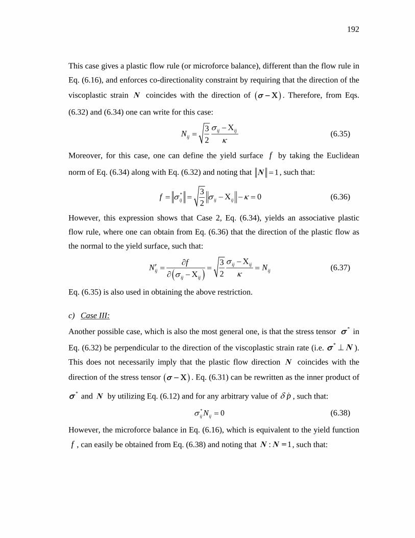
192
This case gives a plastic flow rule (or microforce balance), different than the flow rule in
Eq. (6.16), and enforces co-directionality constraint by requiring that the direction of the
viscoplastic strain N coincides with the direction of . Therefore, from Eqs.
(6.32) and (6.34) one can write for this case:
3
2ij ij
ijN
(6.35)
Moreover, for this case, one can define the yield surface f by taking the Euclidean
norm of Eq. (6.34) along with Eq. (6.32) and noting that 1N , such that:
* 30
2ij ij ijf (6.36)
However, this expression shows that Case 2, Eq. (6.34), yields an associative plastic
flow rule, where one can obtain from Eq. (6.36) that the direction of the plastic flow as
the normal to the yield surface, such that:
3
2ij ij
ij ij
ij ij
fN N
(6.37)
Eq. (6.35) is also used in obtaining the above restriction.
c) Case III:
Another possible case, which is also the most general one, is that the stress tensor * in
Eq. (6.32) be perpendicular to the direction of the viscoplastic strain rate (i.e. * N ).
This does not necessarily imply that the plastic flow direction N coincides with the
direction of the stress tensor . Eq. (6.31) can be rewritten as the inner product of
* and N by utilizing Eq. (6.12) and for any arbitrary value of p , such that:
* 0ij ijN (6.38)
However, the microforce balance in Eq. (6.16), which is equivalent to the yield function
f , can easily be obtained from Eq. (6.38) and noting that : 1N N = , such that:
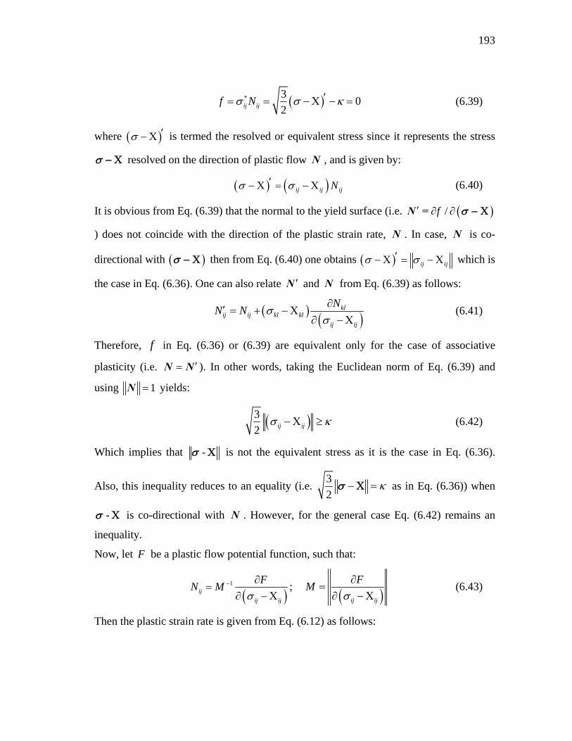
193
* 30
2ij ijf N (6.39)
where is termed the resolved or equivalent stress since it represents the stress
resolved on the direction of plastic flow N , and is given by:
ij ij ijN (6.40)
It is obvious from Eq. (6.39) that the normal to the yield surface (i.e. /f N =
) does not coincide with the direction of the plastic strain rate, N . In case, N is co-
directional with then from Eq. (6.40) one obtains ij ij which is
the case in Eq. (6.36). One can also relate N and N from Eq. (6.39) as follows:
kl
ij ij kl kl
ij ij
NN N
(6.41)
Therefore, f in Eq. (6.36) or (6.39) are equivalent only for the case of associative
plasticity (i.e. N N ). In other words, taking the Euclidean norm of Eq. (6.39) and
using 1N yields:
3
2 ij ij (6.42)
Which implies that - is not the equivalent stress as it is the case in Eq. (6.36).
Also, this inequality reduces to an equality (i.e. 3
2 as in Eq. (6.36)) when
- is co-directional with N . However, for the general case Eq. (6.42) remains an
inequality.
Now, let F be a plastic flow potential function, such that:
1ij
ij ij
FN M
; ij ij
FM
(6.43)
Then the plastic strain rate is given from Eq. (6.12) as follows:

194
13
2vpij
ij ij
FM p
(6.44)
The constraint between the plastic potential F and the yield surface function f can be
obtained by substituting Eq. (6.43) into Eq. (6.38) along with Eq. (6.32), such that:
2
03ij ij
ij ij
Ff M
(6.45)
Differentiating both sides of Eq. (6.45) with respect to the ij ij yields:
2
0kl kl
ij ij ij kl kl ij ij
f F F
(6.46)
Eq. (6.46) provides the relationship between the yield function f and the viscoplastic
potential function F for nonassociative/associative plasticity/viscoplasticity theories.
This relationship is general and can be used for both associative and non-associative
plasticity/viscoplasticity theories.
As it was discussed earlier, in the associative viscoplasticity theories, the yield
function f and the plastic potential function F are assumed to be the same or,
equivalently, the direction of the plastic flow is normal to the yield surface (i.e.
/ /F f N = . According to Eq. (6.46) the assumption of the
associative viscoplasticity requires the second term in the right side of Eq. to be zero,
such that:
2
0kl kl
kl kl ij ij
F
; when f F (6.47)
Or equivalently from Eq. (6.41):
0ij
kl kl
kl kl
N
when f F
N N
(6.48)
which means that
N
as the basic assumption for associative
plasticity/viscoplasticity theories. Therefore, one can conclude that Eq. (6.46) governs

195
the relation between the yield function and the viscoplastic potential function for both
associative and non-associative viscoplasticity theories. It should be mentioned that this
equation naturally implies that the yield surface and the plastic potential functions are
the same for associative viscoplasticity theories.
Eqs. (6.43), (6.45), and (6.46) are derived when both isotropic and kinematic
hardening are assumed. These equations are simplified to the following forms when
kinematic hardening is not considered.
1ij
ij
FN M
; ij
FM
(6.49)
2
03ij
ij
Ff M
(6.50)
2
0kl
ij ij kl ij
f F F
(6.51)
It should be noted that the same arguments can be used for deriving associative
and non-associative damage rules.
The above arguments clearly show the existence of a constraint between the yield
function f and the plastic potential F in a thermodynamically consistent framework.
The yield surface f can be derived directly using the microforce balance without the
need for any further assumption more than the Helmholtz free energy function and the
rate of the energy dissipation that will be shown in the subsequent development. On the
other hand, one may solve the differential equation presented in Eq. (6.46) for
thermodynamically admissible potential functions once the yield function is known.
Reversely, one can use the given plastic potential function to derive its associated
thermodynamically admissible yield function f . The second approach is used in this
work to derive the thermodynamically consistent yield functions associated with the
given plastic potential function.

196
6.3.4. Internal State Variables and Clausius-Duhem Inequality
The Helmholtz free energy is assumed to be a function of the following variables in the
healing configuration:
( , , , , , )veij m p h T (6.52)
The internal state variables associated with the viscoelastic process are considered as the
hidden variables. Ideally speaking, these hidden variables can be used to relate the
developed constitutive equation at continuum scale to the microstructure.
By combining the first and second laws of thermodynamics (i.e. balance of
energy and entropy imbalance, respectively) and also assuming that the material density
does not change during the deformation (i.e. 0 ), the Clausius-Duhem inequality for
non-isothermal conditions can be written as follows (c.f. Lemaître and Chaboche, 1990):
, ext int
1i iT q T dV P P
T
(6.53)
Substituting Eq. (6.7) into Eq. (6.53) and noting that the sub-region is arbitrary yield
the following local form of the Clausius-Duhem inequality:
int
,1
10
veMve vp
ij ij m m ij ij i im
p T q TT
(6.54)
which defines the rate of the energy dissipation per unit volume, . However, the
thermodynamic forces conjugate to the damage density and healing variable (i.e. Y and
H ) are null according to Eqs. (6.17) and (6.18). Hence, these terms can be added Eq.
(6.54) without changing the values of the rate of energy dissipation per unit volume. As
it will be shown, adding these null terms will substantially simplify the derivation of the
damage and healing conditions. Hence, one can rewrite Eq. (6.54) as:
int
,1
10
veMve vp
ij ij m m ij ij i im
p Y Hh T q TT
(6.55)
Substituting the time derivative of the Helmholtz free energy into Eq. (6.55) yields:

197
int
1
,
1 0
veMve vp
ij ij m m ij ijve vpmij ijm
i ip Y H h T q Tp h T T
(6.56)
From Eq. (6.56) the following classical thermodynamic state law for entropy is defined:
T
(6.57)
such that the rate of the energy dissipation from Eqs. (6.56) and (6.57) can be written as:
int
1
,
1 0
veMve vp
ij ij m m ij ijve vpmij ijm
i ip Y H h q Tp h T
(6.58)
However, in order to obtain non-zero dissipation resulting from the viscoelasticity,
viscoplasticity, and viscodamage dissipative processes, the following energetic
thermodynamics conjugate forces that depend on the Helmholtz free energy are defined
from Eq. (6.58), such that:
eneij ve
ij
(6.59)
enem
m
; int1,..., vem M (6.60)
eneij vp
ij
(6.61)
ene
p
(6.62)
eneY
(6.63)
eneHh
(6.64)
where “ene” designates the energetic component of the thermodynamic conjugate forces.
Substituting Eqs. (6.59)-(6.64) into Eq. (6.58) implies:

198
intene ene ene ene
1
ene ene,
1 0
veMve vp
ij ij ij m m m ij ij ijm
i i
p
Y Y H H h q TT
(6.65)
Eq. (6.65) shows that the rate of energy dissipation resulting from different
mechanisms (i.e. viscoelasticity, viscoplasticity, viscodamage, and healing) is positive
only if the thermodynamic conjugate forces have dissipative components as well. Hence,
rewriting Eq. (6.65) implies:
int
dis dis dis dis dis dis,
1
10
veMve vp
ij ij m m ij ij i im
p Y H h q TT
(6.66)
where “dis” designates the dissipative component of the thermodynamic conjugate
forces and defined as follows:
dis eneij ij ij (6.67)
dis enem m m ; int1,..., vem M (6.68)
dis eneij ij ij (6.69)
dis ene (6.70)
dis eneY Y Y (6.71)
dis eneH H H (6.72)
Therefore, in the current work, the energetic means that the thermodynamic conjugate
forces are derived from the Helmholtz free energy function and the dissipative means
that they are derived from the dissipation potential. Therefore, in order to formulate
constitutive equations for the energetic and dissipative conjugate forces, one needs to
know: (1) how the material stores energy which helps in assuming a mathematical form
for the Helmholtz free energy, and (2) how the material dissipates energy which helps in
assuming a mathematical form for the rate of energy dissipation. Furthermore, the rate of
energy dissipation [Eq. (6.58)] naturally enforces the decomposition of the stress tensor
into energetic and dissipative components. This decomposition results in a more
comprehensive relation between the stress and the viscoelastic strain compared to the

199
classical relations for the viscoelastic materials. It is noteworthy to mention that, the
Clausius-Duhem inequality also enforces the decomposition of the specific entropy
into energetic specific entropy (i.e. ene
T
) and the dissipative specific entropy (i.e.
dis ene ) which is related directly to the rate of energy dissipation. However, this
decomposition is not used for the specific entropy in this work and the classical
thermodynamic law is assumed for entropy as in Eq. (6.57) with dis 0 .
Let one assume for a moment that neither damage nor viscoplasticity occur in the
material (i.e. 0p and 0 ) in order to explain the common argument that has been
made in the literature for substituting the total stress instead of its energetic component
in Eq. (6.59) [c.f. Levesque et al. (2008)]. Therefore, assuming isothermal conditions as
well, the Clausius-Duhem inequality in Eq. (6.58) reduces to the following form:
int
1
0veM
veij ij m mve
mij m
(6.73)
The commonly used argument states that the Clausius-Duhem inequality [Eq. (6.73)] is
valid for all load histories. So, let the load history to be a hypothetical reversible load
history such that the viscoelastic internal state variables remain constant (i.e. 0m ).
Under this load history the second term of the inequality in Eq. (6.73) vanishes and the
following constitutive law is obtained:
ij veij
(6.74)
However, the authors believe that this argument is not consistent. The reason is that the
material is assumed to be viscoelastic, and hence, the state variables m are not
independent of the viscoelastic strains ve and they evolve even under the unloading
process. In other words, both ve and m evolve during the viscoelastic process whether
it is loading or unloading. Hence, a more consistent framework is to admit the
decomposition of the stress tensor into energetic and dissipative components as in Eq.

200
(6.67) such that Eq. (6.74) defines the thermodynamic law for the energetic component.
The thermodynamic laws for the dissipative components are derived next.
6.3.5. Maximum Rate of the Energy Dissipation Principle
As it was shown in the previous section, the correct estimation of the rate of the energy
dissipation requires the decomposition of the thermodynamic conjugate forces into
energetic and dissipative components (Ziegler, 1977, 1983; Ziegler and Wehrli, 1987;
Fremond and Nedjar, 1996; Shizawa and Zbib, 1999; Gurtin, 2003; Anand et al., 2005;
Gurtin and Anand, 2005; Abu Al-Rub et al., 2007; Gurtin and Anand, 2009; Lele and
Anand, 2009; Voyiadjis and Deliktas, 2009). However, in all of these works, except for
the works of Ziegler (1977, 1983) and Shizawa and Zbib (1999), the constitutive
equations for the dissipative components are merely constitutive assumptions and are not
derived based on the laws of thermodynamics. However, in this work, the dissipative
components of thermodynamic conjugate forces are determined directly from the rate of
energy dissipation by using the maximum energy dissipation principle. Eq. (6.66)shows
that the rate of the energy dissipation can be decomposed into its thermo-viscoelastic,
thermo-viscoplastic, thermo-viscodamage, thermo-healing, and thermal components,
such that:
0tve tvp tvd tH th (6.75)
where tve , tvp , tvd , tH , and th are thermo-viscoelastic, thermo-viscoplastic,
thermo-viscodamage, thermo-healing, and thermal components of the rate of the energy
dissipation, respectively, which are given as follows:
int
dis dis
1
0veM
tve veij ij m m
m
(6.76)
dis dis 0tvp vpij ij p (6.77)
dis 0tvd Y (6.78)
dis 0tH H h (6.79)
,
10th
i iq TT
(6.80)

201
Obviously, Eqs. (6.76)-(6.80) are more restrict constraints for obtaining a positive-
definite dissipation than that in Eq.(6.75). Now, constraint conditions are needed in order
to maximize the rate of energy dissipation. This can be achieved by defining the
following constraint conditions:
int
dis dis
1
0veM
tve tve veij ij m m
m
D
(6.81)
dis dis 0tvp tvp vpij ijD p (6.82)
dis 0tvd tvdD Y (6.83)
dis 0tH tHD H h (6.84)
,
10th th
i iD q TT
(6.85)
Hence, the following objective functions tve , tvp , tvd , tH , and th with their
corresponding Lagrange multipliers tve , tvp , tvd , tH , and th subjected to the
constraint 0tveD , 0tvpD , 0tvdD , 0tHD , and 0thD , respectively, are defined,
such that:
tve tve tve tveD (6.86)
tvp tvp tvp tvpD (6.87)
tvd tvd tvd tvdD (6.88)
tH tH tH tHD (6.89)
th th th thD (6.90)
Maximizing the above objective functions by using the necessary conditions implies:
0tve
veij
; 0
tve
m
; 0
tvp
vpij
; 0
tvp
p
; 0
tvd
; 0tH
h
;
0
/
th
iq T
(6.91)
Substituting Eqs. (6.86)-(6.90) into Eq. (6.91) yield the following conjugate laws for the
dissipative forces, such that:
distve
tveij ve
ij
(6.92)

202
distve
tvem
m
(6.93)
distvp
tvpij vp
ij
(6.94)
distvp
tvp
p
(6.95)
distvd
tvdY
(6.96)
distH
tHHh
(6.97)
, /
thth
ii
Tq T
(6.98)
where
1 1 1 1 1
1 ; 1 ; 1 ; 1 ; 1tve tvp tvd tH thtve tvp tvd tH th
(6.99)
By substituting Eqs. (6.92)-(6.98) respectively into Eqs. (6.81)-(6.85), the Lagrange
multipliers in Eq. (6.99) can be determined as:
int
1
ve
tvetve
Mtve tveveij mve
mij m
(6.100)
tvp
tvptvp tvp
vpijvp
ij
pp
(6.101)
tvd
tvdtvd
(6.102)
tH
tHtH
hh
(6.103)

203
/
thth
thi
i
q
q T T
(6.104)
It is noteworthy that other constraints such as the viscoplastic microforce balance
[Eq.(6.24)], the viscodamage microforce balance [Eq. (6.17)], the healing microforce
balance [Eq. (6.18)], and the viscoelastic microforce balance [Eq. (6.25)] can also be
applied to the objective functions which requires determination of several Lagrange
multipliers. Although applying more constraints to the objective function results in a
more comprehensive solution for dissipative components of the thermodynamic
conjugate forces, it makes the problem more complex. This section concludes the
general thermodynamic framework for determining the energetic and dissipative
components of thermodynamic conjugate forces. The next following sections present the
capabilities of the presented thermodynamic framework through an example that derives
a temperature-dependent viscoelastic, viscoplastic, viscodamage, and healing
constitutive model for time- and rate-dependent materials.
6.4. Application to Bituminus Materials
In this section, the thermodynamic framework explained in the previous sections will be
used to derive a thermo-viscoelastic, thermo-viscoplastic, thermo-viscodamage, and
thermo-healing constitutive equations for time- and rate-dependent materials. The
objective is to derive thermodynamic consistent Schapery-type viscoelastic law,
Perzyna-type viscoplastic law, damage law proposed by Darabi et al. (2011c), and a
healing law suitable for time- and rate-dependent materials.
The Helmholtz free energy is decomposed into thermo-viscoelastic, thermo-
viscoplastic, thermo-viscodamage, and healing components, such that:
( , , , , , , ) ( , , ) ( , , )
( , ) ( , )
ve vp tve ve tvp vpij m ij ij m ij
tvd tH
p h T T p T
T h T
(6.105)
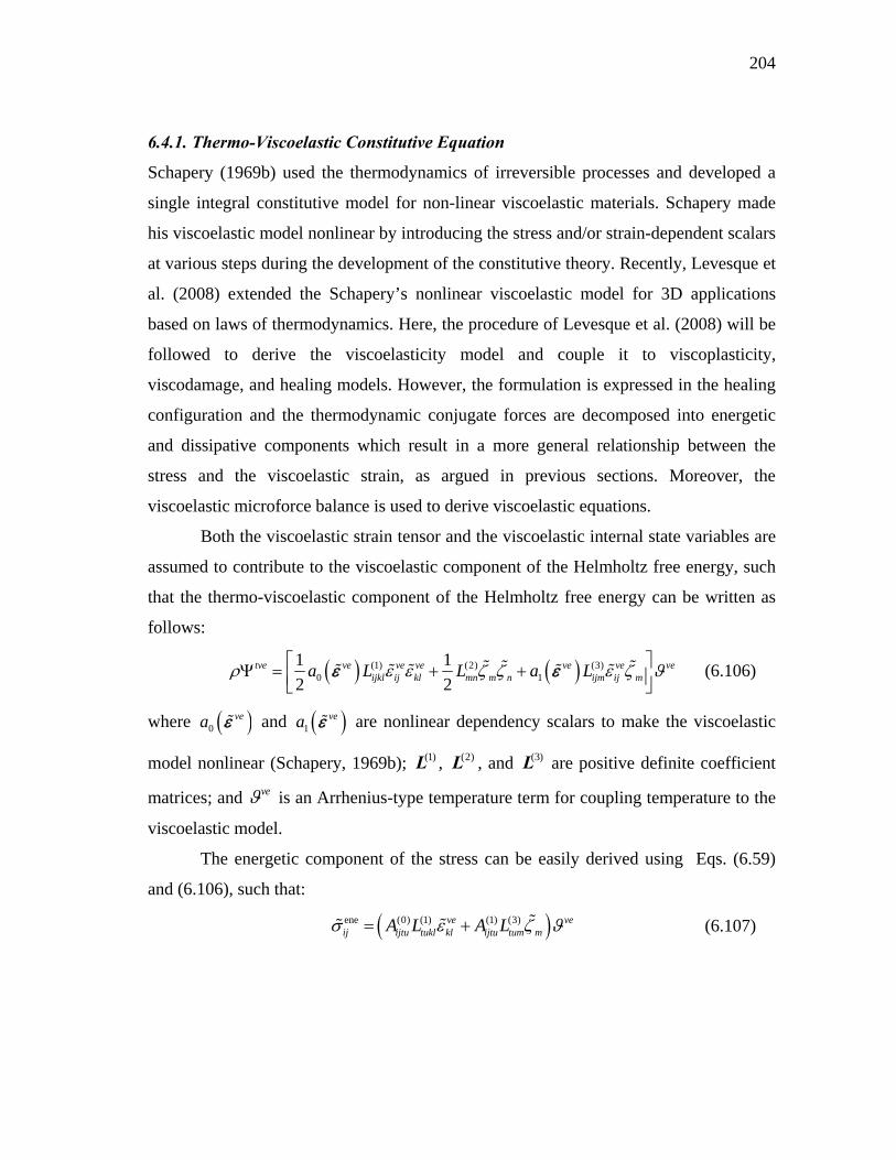
204
6.4.1. Thermo-Viscoelastic Constitutive Equation
Schapery (1969b) used the thermodynamics of irreversible processes and developed a
single integral constitutive model for non-linear viscoelastic materials. Schapery made
his viscoelastic model nonlinear by introducing the stress and/or strain-dependent scalars
at various steps during the development of the constitutive theory. Recently, Levesque et
al. (2008) extended the Schapery’s nonlinear viscoelastic model for 3D applications
based on laws of thermodynamics. Here, the procedure of Levesque et al. (2008) will be
followed to derive the viscoelasticity model and couple it to viscoplasticity,
viscodamage, and healing models. However, the formulation is expressed in the healing
configuration and the thermodynamic conjugate forces are decomposed into energetic
and dissipative components which result in a more general relationship between the
stress and the viscoelastic strain, as argued in previous sections. Moreover, the
viscoelastic microforce balance is used to derive viscoelastic equations.
Both the viscoelastic strain tensor and the viscoelastic internal state variables are
assumed to contribute to the viscoelastic component of the Helmholtz free energy, such
that the thermo-viscoelastic component of the Helmholtz free energy can be written as
follows:
(1) (2) (3)0 1
1 1
2 2tve ve ve ve ve ve ve
ijkl ij kl mn m n ijm ij ma L L a L (6.106)
where 0vea and 1
vea are nonlinear dependency scalars to make the viscoelastic
model nonlinear (Schapery, 1969b); (1)L , (2)L , and (3)L are positive definite coefficient
matrices; and ve is an Arrhenius-type temperature term for coupling temperature to the
viscoelastic model.
The energetic component of the stress can be easily derived using Eqs. (6.59)
and (6.106), such that:
ene (0) (1) (1) (3)ve veij ijtu tukl kl ijtu tum mA L A L (6.107)

205
where (0)ijtuA and (1)
ijtuA are nonlinear parameters related to the instantaneous and transient
viscoelastic responses, respectively which are no longer an scalar for 3D models, such
that:
(0) 00
1
2ve
ijtu it ju tuveij
aA a
; (1) 11
veijtu it ju tuve
ij
aA a
(6.108)
Eq. (6.108) shows that the energetic component of the stress has two terms, one of which
is related to instantaneous response and the other one is related to the recoverable
processes associated with the viscoelastic internal state variables. These two terms are
recovered upon the unloading and no energy dissipates due to these terms. However, the
dissipation mechanism results from the viscoelastic strain rate and the rate of the
viscoelastic internal state variables which are related to the chain mobility and friction
between the polymer chains. In this work, a simple quadratic form is postulated for the
viscoelastic component of the rate of energy dissipation, such that:
tve ve ve veijkl ij kl mn m nP
(6.109)
Parameters in Eq. (6.109) are defined as follows:
2 tve
ijkl ve ve veij kl
; 2 tve
mn vem n
P
(6.110)
The same Arrhenius-type temperature coupling terms are assumed for both temperature-
dependent Helmholtz free energy and rate of energy dissipation. However, different
temperature coupling terms can be assumed for the Helmholtz free energy and the rate of
energy dissipation. The assumed form for the thermo-viscoelastic component of rate of
energy dissipation guarantees the rate of the energy dissipation to be always positive.
Another common assumption in the theory of nonlinear viscoelasticity is that the
thermodynamic conjugate forces can be expressed as a nonlinear function of the
evolution of the state variables (see e.g. Schapery, 1969a; Levesque et al., 2008).
However, as it will be shown here, there is no need to make these assumptions and the
viscoelastic laws can be derived directly using the viscoelastic microforce balance [Eq.
(6.25)]. The viscoelastic microforce balance indicates that the summation of the

206
energetic and dissipative components of the thermodynamic forces conjugate to the
viscoelastic internal state variables is zero, such that:
ene dis0 0m m m (6.111)
The energetic and dissipative components of the viscoelastic conjugate forces can be
determined using Eqs., (6.60), (6.93), (6.100), (6.106), and (6.109), such that:
ene (2) (3)1
ve ve vem mn n ijm ijL a L
; dis vem mn nP
(6.112)
Substituting Eq. (6.112) into Eq. (6.111) implies:
(2) (3)1 0ve ve
mn n mn n ijm ijP L a L (6.113)
Eq. (6.113) is the partial differential equation governing the viscoelastic processes. This
equation relates the viscoelastic internal state variables to the viscoelastic strain tensor.
Eq. (6.113) represents a coupled system of differential equations which expresses the
evolution of internal variables n as a function of veij . Expressing Eq. (6.113) in a basis
where the coefficient matrices are diagonal and using the Laplace transform implies:
(3)
1(2) 0( ) 1 exp[ ( )]
tijm vem m ij
mm
L dt t a d
L d
; No sum on m (6.114)
where (2)mm
mmm
L
P . Eq. (6.114) shows the relation between the viscoelastic state variables
and the viscoelastic strain. It is clear from Eq. (6.114) that the viscoelastic state variables
m depend on the viscoelastic deformation history veij . Hence, the viscoelastic internal
state variables evolve with the evolution of the viscoelastic strain. This supports the
previously made argument for decomposing the total stress into its energetic and
dissipative components. Also, Eq. (6.114) shows that the assumptions of assuming state
variables m to be constant (i.e. 0m ) is valid only when the viscoelastic strain is
constant (i.e. 0veij ) which happens only in the absence of the viscoelastic processes.
Hence, it is not consistent to make this argument to derive a viscoelasticity law as
presented by several researchers (Levesque et al., 2008).

207
The dissipative component of the stress can now be obtained using Eqs. (6.92) and
(6.109), such that:
distve
tve veij ijkl klve
ij
(6.115)
The stress as a function of the viscoelastic strain can now be obtained by substituting
Eqs. (6.107), (6.114), and (6.115) into Eq. (6.67), such that:
(0) (0)
(2)
(1) ( )
01
1 exp[ ( )]
ve ve veij ijkl kl ijtu tukl kl
veMt klve mijtu tukl m
m
G E
d gG E t d
d
(6.116)
where
(3)(0) (0) (0) (1) (1) (3)
1 (2)
(3) (3)(1) (1) ( ) (2)
1(2)
;
; ;
klmijtu tukl ijtu tukl ijtu tum
mm
m tum klmijtu ijtu tukl
mm
LG E A L a A L
L
L LG A E g a
L
(6.117)
Eq. (6.116) represents a more comprehensive formulation that relates the total stress to
the viscoelastic strain comparing to Levesque et al. (2008). According to notations of
Duvaut and Lions (1976), the first two terms in the right hand side of Eq. (6.116) refer to
the viscoelastic materials with the short memories since these two terms relate the state
of stress at time t only to the strains at current time t and the immediately preceding
time. However, the third term in the right hand side of Eq. (6.116) corresponds to the
viscoelastic materials with long term memory since it relates the state of stresses at time
t to strains at the times preceding t . For the case of linear viscoelasticity the nonlinear
parameters should be always unity (i.e. (0) (1) G G I and (2) 1g ).
Eq. (6.116) clearly shows that the temperature-dependency can easily be
incorporated into the viscoelastic models using a temperature coupling term for all terms
in the right hand side of Eq. (6.116). This approach is more general comparing to the
classical Schapery-type viscoelasticity where the temperature shift factor is introduced in
the definition of reduced time. The reason is that incorporation of the temperature shift
factor as part of the reduced time variable only makes the third term in the RHS of Eq.

208
(6.116) temperature-dependent. However, using the Arrhenius-type temperature
coupling term makes all terms of Eq. (6.116) to depend on temperature. Moreover, as it
was mentioned earlier, two temperature coupling terms can be introduced in Eq. (6.116),
one is related to Helmholtz free energy affecting the instantaneous response and the
other is related to the rate of energy dissipation affecting the rate-type and the transient
responses. Furthermore, using ve implies that the nonlinear parameters (0)G , (1)G , and
(2)g are not temperature-dependent which makes their calibration easier. It is
noteworthy that a proper viscoelastic model can be derived for a specific material by
postulating different mathematical forms for viscoelastic components of Helmholtz free
energy and rate of energy dissipation.
6.4.2. Thermo-Viscoplastic Constitutive Equation
In the classical theory of continuum plasticity/viscoplasticity several experimentally
motivated assumptions should be made to formulate a plasticity/viscoplasticity theory.
These assumptions are the mathematical forms for yield surface and plastic potential
function from which the plastic strain is determined. Most of the times these
assumptions are made based on experimental observations. Hence, there is no guarantee
for these experimental assumptions to satisfy fundamental laws of thermodynamic. As it
was mentioned in the introduction, several researchers have tried to derive the plasticity
yield surface based on the fundamental laws of thermodynamics (Gurtin, 2003; Anand et
al., 2005; Gurtin and Anand, 2005; Abu Al-Rub et al., 2007; Gurtin et al., 2007;
Voyiadjis and Abu Al-Rub, 2007; Abu Al-Rub, 2008a, b; Gurtin, 2008; Gurtin and
Anand, 2009). However, to the authors’ best knowledge they could only derive the von-
Misses-type associative plasticity/viscoplasticity theory (i.e. the 2J -flow theory). In this
section, the generalized non-associative viscoplasticity yield conditions and potential
functions will be derived based on the viscoplastic microforce balance. Both isotropic
and kinematic hardening terms are considered. Also, an evolution equation similar to
Armstrong and Frederick model (1966) is derived using the presented thermodynamic
framework.

209
T non-associative viscoplasticity can be derived based on principle of virtual
power. Eq. (6.45) represents the relationship between the yield surface and the plastic
potential function. In this section, the thermodynamically consistent dynamic yield
surface associated with a given viscoplastic potential function will be derived. As it is
shown in this section, Eq. (6.45) naturally yields to non-associative viscoplasticity for
the given viscoplastic potential. The normality rule for non-associative plasticity in the
healing configuration which states that the direction of the viscoplastic strains in the
effective configuration is normal to the viscoplastic potential function is used. Hence,
there exists a viscoplastic potential function F for which the direction of the
viscoplastic flow in the healing configuration, N , in Eq. (6.43) can be defined as:
1
ij
ij ij
FN M
; ij ij
FM
(6.118)
Comparing Eqs. (6.26)and (6.118) implies:
13 3
2 2vpij ij
ij ij
FpN pM
(6.119)
Eq. (6.119) properly relates N and ij ij
F
. The modified Drucker-Prager-type
[see Eqs. (2.23) and (2.25)] is expressed in the healing configuration and assumed as the
viscoplastic function, such that:
1vpF I (6.120)
Substituting Eq. (6.120) into Eq. (6.118) implies:
1 1
2
12 32
2
3 1 3 11 1
4 2 3
1 9 3
4 2
ij ijij ijvp vp
vp
ik ik kj kj ij ijvp
SN A A
d dJ
dA J S S J S
d J
(6.121)
where

210
2 22
33/22
2 23
2 32 2
3 1 27 1 31 1 1
8 3 4
3 3 1 3 1 1
4
1 81 1 9
16
vp vp vp
vp vp
ik ik kj kj im im mj mj
vp
Ad d d
J
d d J
S S S S J
d J J
(6.122)
Substituting Eq. (6.122) into the equation of microforce balance yields:
1 0vp I A (6.123)
Eq. (6.123) shows the expression of the yield surface associated with the assumed
viscoplastic potential function in Eq. (6.120). It is noteworthy that the term A can be
considered as the hardening function. Interestingly, Eq. (6.122) shows that the hardening
function associated with this plastic potential function is stress dependent.
It should be mentioned that one of the common ways to obtain viscoplasticity
theories is to treat Eq. (6.123) as the rate-independent plasticity yield surface and extend
it to rate-dependent plasticity (viscoplasticity) using the overstress concept (Zener and
Hollomon, 1944; Malvern, 1951; Perzyna, 1986; Perzyna and Korbel, 1998). According
to this approach, the extension of the plasticity yield surface to the rate-dependent
plasticity (viscoplasticity) theory is usually accompanied by the assumption that the
stress state is no longer on the yield surface. Hence, an overstress function is defined in a
dynamic yield surface to constrain the stress state to remain on the dynamic yield
surface. Then by defining an admissible form of the plasticity Lagrange multiplier as a
function of the overstress, the dynamic yield surface can be obtained (see Voyiadjis et
al., 2004 for more details). However, it will be shown here that there is no need for
extending Eq. (6.123) to viscoplasticity. In other words, the viscoplasticity dynamic
yield surface obtains directly from Eq. (6.123) if the hardening parameter is properly
decoupled into its energetic and dissipative components (i.e. ene dis ). The next
step is to postulate mathematical forms for the thermo-viscoplastic component of the
Helmholtz free energy tvp and the rate of thermo-viscoplastic energy dissipation tvp

211
in order to define the dynamic yield surface for the assumed viscoplastic potential. The
following forms are postulated for these two functions:
1 0 1 22
1 1exp( )
2tvp vp vp vp
ij ijC p p p T
(6.124)
1
1
2 3
1exp
2
Ntvp vp vp vp vp
ij ij vp vp
pC p C T
(6.125)
The energetic and dissipative components of the isotropic and kinematic hardening can
be obtained using Eqs. (6.61), (6.62), (6.94), (6.95), (6.124), and (6.125), such that:
ene0 1 21 exp( ) vpp ;
1
dis3
N
vp vp
pC
(6.126)
ene1
vp vpij ijC ; dis
2 exp vp vpij ijC p (6.127)
Therefore, the total isotropic and kinematic hardening functions will be expressed as:
1
0 1 2 31 exp( )N
vpvp vp
pp C
(6.128)
1 2 expvp vp vpij ij ijC C p
(6.129)
The dynamic viscoplastic yield function associated with the assumed viscoplastic
potential can now be obtained using Eqs. (6.123), (6.128), and (6.129), such that:
1
1 0 1 2 31 exp( ) 0N
vp vpvp vp
pI p A C A
(6.130)
Eq. (6.130) represents the temperature-dependent dynamic yield surface associated with
the assumed viscoplastic potential [Eq. (6.120)].
Taking the time derivative of Eq. (6.127) at the reference temperature and
neglecting the temperature evolution yield:
ene1
vpij ijC ; dis
2 2exp expvp vpij ij ijC p p C p (6.131)
Adding both sides of Eqs. (6.131)1 and (6.131)2 implies:
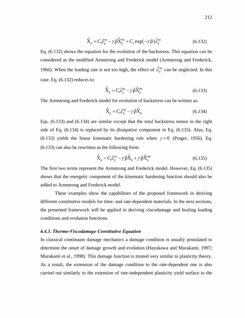
212
dis1 2 expvp vp
ij ij ij ijC p C p (6.132)
Eq. (6.132) shows the equation for the evolution of the backstress. This equation can be
considered as the modified Armstrong and Frederick model (Armstrong and Frederick,
1966). When the loading rate is not too high, the effect of vpij can be neglected. In this
case. Eq. (6.132) reduces to:
dis1
vpij ij ijC p (6.133)
The Armstrong and Frederick model for evolution of backstress can be written as:
1vp
ij ij ijC p (6.134)
Eqs. (6.133) and (6.134) are similar except that the total backstress tensor in the right
side of Eq. (6.134) is replaced by its dissipative component in Eq. (6.133). Also, Eq.
(6.133) yields the linear kinematic hardening rule when 0 (Prager, 1956). Eq.
(6.133) can also be rewritten as the following form:
ene1
vpij ij ij ijC p p (6.135)
The first two terms represent the Armstrong and Frederick model. However, Eq. (6.135)
shows that the energetic component of the kinematic hardening function should also be
added to Armstrong and Frederick model.
These examples show the capabilities of the proposed framework in deriving
different constitutive models for time- and rate-dependent materials. In the next sections,
the presented framework will be applied in deriving viscodamage and healing loading
conditions and evolution functions.
6.4.3. Thermo-Viscodamage Constitutive Equation
In classical continuum damage mechanics a damage condition is usually postulated to
determine the onset of damage growth and evolution (Hayakawa and Murakami, 1997;
Murakami et al., 1998). This damage function is treated very similar to plasticity theory.
As a result, the extension of the damage condition to the rate-dependent one is also
carried out similarly to the extension of rate-independent plasticity yield surface to the

213
dynamic viscoplasticity yield surface (Voyiadjis et al., 2004). However, here it will be
shown that the rate-dependent damage (viscodamage) condition can be derived directly
from the principle of virtual power and laws of thermodynamics. Eq. (6.17) defines the
damage microforce balance. It will be shown here that the damage microforce balance is
in fact the damage condition. Combining the damage microforce balance with Eq.
(6.71) yields:
ene dis ene dis0 0 Y Y Y Y Y (6.136)
where eneY and disY are given in Eqs. (6.63) and (6.96), respectively. To the best of the
authors knowledge, this interesting result has been reported here for the first time. In
fact, Eq. (6.136) is the damage condition criterion. Based on the mathematical form of
thermo-viscodamage Helmholtz free energy tvd and rate of thermo-viscodamage
energy dissipation tvd the damage condition can be rate-independent or rate-
dependent. Wu et al. (2006) proposed an energy-based plastic-damage model for
concrete in which the Helmholtz free energy in the presence of damage is expressed as a
function of stress invariants and damage variable. Similar assumptions have been made
by Voyiadjis et al. (2004), Voyiadjis and Abu Al-Rub (2006), and Abu Al-Rub and Kim
(2009). Therefore, the following form is postulated for the thermo-viscodamage
component of the Helmholtz free energy to consider the confinement effects, the
different effects of damage in tensile and compressive loading conditions, and the effect
of temperature on damage evolution and growth, such that:
13
1 2
111 exp
vdtvd vd
eff
b Ib
b b
(6.137)
This form is postulated in order to derive the viscodamage model proposed by Darabi et
al. (2011c) [see Chapters II and III for more information]. The energetic component of
the viscodamage force can now be determined using Eqs. (6.63) and (6.137), such that:
1ene 13
2
11 expvd
vdeff
b IY b
b
(6.138)

214
An expression similar to that assumed for the thermo-viscoplastic rate of energy
dissipation is postulated for the rate of the thermo-viscodamage energy dissipation tvd ,
such that:
11
0
qtvd vd
vd vdb
(6.139)
Then, the dissipative component of the damage thermodynamic force disY can be
obtained using Eqs. (6.96) and (6.139) as follows:
1
dis 0q
vd vd vd
bY
(6.140)
with 11 1/tvd q
. The rate-dependent damage surface can be determined by
substituting Eqs. (6.138) and (6.140) into Eq. (6.136), such that:
1
1 013
2
11 exp 0vd q
vdeff vd vd vd
b bIb
b
(6.141)
Eq. (6.141) represents the dynamic viscodamage loading condition for temperature- and
rate-dependent damage (thermo-viscodamage). This equation can also be represented as
a damage evolution law, such that:
1
1
32 0
11exp
qvd
vd vdeff
bI
b qb b
(6.142)
where 2 1qvd vd
. A simplified version of Eq. (6.142) has applied to predict the
time- and rate-dependent damage response of asphalt mixes [Refer to Chapter II and
Darabi et al. (2011c) for more details].
6.4.4. Thermo-Healing Constitutive Equation
As it was mentioned in the introduction part, some engineering materials have the
potential to heal and retrieve part of their strength and stiffness with time. Hence, a
robust continuum based model should be able to predict the healing process in addition

215
to the damage evolution and growth. Here, it is shown that the healing evolution law can
easily be obtained from the principle of virtual power. In fact, the defined healing
microforce balance [Eq. (6.18)] is the balance law governing the healing process in the
materials. The healing microforce balance states that the summation of the energetic and
dissipative components of the healing force should be zero, such that:
ene dis ene dis0 0 H H H H H (6.143)
where eneH and disH are given in Eqs. (6.64) and (6.97), respectively. To the best of the
authors knowledge, this interesting result has been reported here for the first time. In
fact, the healing evolution can be easily obtained using Eq. (6.143). Different forms for
the healing evolution law can be obtained based on the mathematical form of thermo-
healing Helmholtz free energy tH and the rate of thermo-healing energy dissipation
tH . In this work, mathematical forms are assumed for the healing components of the
Helmholtz free energy and rate of energy dissipation in order to derive the healing model
proposed by Abu Al-Rub et al. (2010a) to model fatigue damage in bituminous
materials. To achieve this, the following forms are postulated for the healing
components of the Helmholtz free energy and rate of energy dissipation, such that:
1 1 ,ene1
1
11
1ktH Hh
k
(6.144)
2 2 ,dis2 1
ktH Hh (6.145)
where ,eneH and ,disH are Arrhenius-type temperature coupling terms to couple
temperature to the energetic and dissipative components of the healing model. Note that
the material parameters 1 and 2 could depend on surface energy since they capture the
changes in the total surface energy because of the healing of micro-cracks. Moreover,
the healing component of the rate of energy dissipation is expressed as a function of
healing rate and damage history. Although the healing component of the rate of energy
dissipation depends on the damage density, it does not contribute to the dissipative
component of the damage force. Energetic and dissipative components of the healing
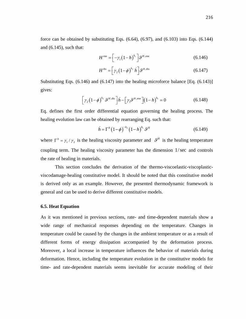
216
force can be obtained by substituting Eqs. (6.64), (6.97), and (6.103) into Eqs. (6.144)
and (6.145), such that:
1ene ,ene1 1
k HH h (6.146)
2dis ,dis2 1
k HH h (6.147)
Substituting Eqs. (6.146) and (6.147) into the healing microforce balance [Eq. (6.143)]
gives:
2 1,dis ,ene2 11 1 0
k kH Hh h (6.148)
Eq. defines the first order differential equation governing the healing process. The
healing evolution law can be obtained by rearranging Eq. such that:
2 11 1k kh Hh h (6.149)
where 1 2/h is the healing viscosity parameter and H is the healing temperature
coupling term. The healing viscosity parameter has the dimension 1/ sec and controls
the rate of healing in materials.
This section concludes the derivation of the thermo-viscoelastic-viscoplastic-
viscodamage-healing constitutive model. It should be noted that this constitutive model
is derived only as an example. However, the presented thermodynamic framework is
general and can be used to derive different constitutive models.
6.5. Heat Equation
As it was mentioned in previous sections, rate- and time-dependent materials show a
wide range of mechanical responses depending on the temperature. Changes in
temperature could be caused by the changes in the ambient temperature or as a result of
different forms of energy dissipation accompanied by the deformation process.
Moreover, a local increase in temperature influences the behavior of materials during
deformation. Hence, including the temperature evolution in the constitutive models for
time- and rate-dependent materials seems inevitable for accurate modeling of their

217
mechanical responses. In this section, the heat equation necessary for calculating the
increase in temperature due to different deformation processes is derived.
The first law of thermodynamic for a sub-body having the outward unit vector
n normal to the boundary can be written as:
ext exti i
dedV P q n dA r dV
dt
(6.150)
where e and extr are internal energy density and the density of external heat gained by
the body (e.g. through radiation), and extP is the external power which is equal to the
internal power intP . Meanwhile, the internal energy density e the specific entropy
and the Helmholtz free energy density are related through the following relationship:
e T (6.151)
By neglecting the changes in the mass density during the deformation, using the
divergence theorem, noting that the sub-body is arbitrary, using the equivalency of
internal and external expenditures of power, and using the definition of internal
expenditure of power [Eq. (6.7)], the first law of thermodynamic can be rewritten as
follows:
int
, ext1
0veM
ve vpij ij m m ij ij i i
m
T T p Y Hh q r
(6.152)
Substituting Eqs. (6.57) and (6.76)-(6.80) into Eq. (6.152) yields:
ext ,tve tvp tvd tH
i iT r q (6.153)
On the other hand Eqs. (6.57) and (6.105) implies:
tve tvp tvd tH (6.154)
where , , , and tve tvp tvd tH are the specific entropies due to viscoelastic, viscoplastic,
viscodamage, and healing processes, respectively.
tve
tve
T
; tvp
tvp
T
; tvd
tvd
T
; tH
tH
T
(6.155)
The following equations for the specific entropy can be obtained by substituting Eqs.
(6.106), (6.124), (6.137), and (6.144) into Eq. (6.155), such that:

218
(1) (2) (3)0 1
1 1 1
2 2tve ve ve ve ve ve ve
ijkl ij kl mn m n ijm ij ma L L a L Z
(6.156)
1 0 1 22
1 1 1exp( )
2tvp vp vp vp
ij ijC p p p Z
(6.157)
13
1 2
111 exp
vdtvd vd
eff
b Ib Z
b b
(6.158)
1 1 ,ene1
1
1 11
1ktH Hh Z
k
(6.159)
where ZT
. Taking the time derivative of Eq. (6.154) and substitute it in Eq.
(6.153) and using Eqs. (6.59)-(6.64) yield:
,
ene eneene ene ene ene
Thermo-mechanical coupling terms
tve tvp tvd tHp ext i i
ij ijve vpmij m ij
c T r q
Y Hp h T
T T T T T T
(6.160)
where pc TT
is the specific heat at constant pressure. Eq. (6.160) yields a physically
sound relationship for the heat equation. This equation reveals two mechanisms that
contribute to the temperature evolution: (a) the thermo-mechanical coupling terms which
are functions of energetic components of the thermodynamic conjugate forces; and (2)
dissipation terms which are functions of the dissipative components of the
thermodynamic conjugate forces appearing in different components of .
The relationship for the heat flux vector q can be easily determined using the
principle of maximum dissipation. Therefore, an expression is needed for the thermal
component of the rate of energy dissipation in Eq. (6.98). The following form is assumed
for th :
11thij i jk q q
T (6.161)
Substituting Eq. (6.161) into Eq. (6.98) implies:

219
,i ij jq k T (6.162)
with 1/ 2th
. Eq. (6.162) is the well-known Fourier heat conduction law. The negative
sign indicates that the heat flow is opposite to the direction of temperature increase.
6.6. Conclusions
In this work, a general and comprehensive thermodynamic based framework with
especial attention to the decomposition of the thermodynamic conjugate forces into
energetic and dissipative components is presented to derive a temperature-dependent
viscoelastic, viscoplastic, viscodamage, and healing constitutive model for time- and
rate-dependent materials.
The healing natural configuration as the extension of the well-known Kachanov’s
effective (undamaged) configuration is used to enhance the continuum damage
mechanics in modeling the healing phenomenon. Hence, the constitutive models are
presented in the healing configuration which substantially simplifies the numerical
implementation by avoiding the complexities associated with the direct couplings of
viscoelastic and viscoplastic models to the viscodamage and healing models. The power-
correlating hypothesis is used for relating stress and strain tensors in the healing and
damaged configurations. This hypothesis allows one to present the constitutive model in
the healing configuration (for simplicity) and yet to estimate the dissipated energy in the
healed stress space (healed natural configuration) accurately.
Moreover, it is shown that the thermodynamic formulation naturally enforces the
decomposition of the thermodynamic conjugate forces into energetic and dissipative
components. Energetic components are derived using the Helmholtz free energy. A
systematic procedure based on the principle of maximum dissipation (or maximum
entropy production) is presented for deriving dissipative components directly from rate
of energy dissipation. The thermodynamic framework is then used for deriving a more
comprehensive version of Schapery-type viscoelastic model, Perzyna-type viscoplastic
model, and a viscodamage model analogous to the Perzyna-type viscoplastic model, and

220
a healing model for bituminous materials. Moreover, all the derived constitutive models
are coupled to temperature.
Furthermore, it is shown that the principle of virtual power can be used for
deriving generalized non-associative viscoplasticity theories without further needs to
assume a viscoplastic potential function independent from the yield loading condition. It
is also shown that the rate-dependent terms in viscoplasticity dynamic yield surface are
identical to the dissipative components of the hardening function and can be derived
directly from the rate of energy dissipation. Moreover, an equation for the evolution of
the backstress is proposed which can be considered as a modified version of Armstrong
and Frederick model (1966) for the backstress evolution.
The viscoelastic model is derived using the viscoelastic microforce balance,
obtained directly from the principle of virtual power. Similarly, the viscodamage and
healing loading conditions and evolution laws are derived using the viscodamage
microforce balance and healing microforce balance, respectively.
Moreover, the well-known Fourier heat conduction law is derived as a
consequence of decomposing thermodynamic conjugate forces into energetic and
dissipative components and using the principle of maximum dissipation. Finally, the heat
equation for the presented constitutive model is derived.

221
CHAPTER VII
VALIDATION OF THE THERMO-VISCOELASTIC-
VISCOPLASTIC-VISCODAMAGE-HEALING MODEL AGAINST
THE ALF DATA
7.1. Introduction
In this chapter, the presented thermo-viscoelastic-viscoplastic-viscodamage-healing
constitutive models (see Chapters II and V for detailed information on these constitutive
models) is further validated against the FHWA Accelerated Load Facility (ALF) data.
The experimental measurements on ALF materials are performed at North Carolina State
University (NCSU) (see Kim et al., (2008) for a detailed explanation regarding the
material and test procedure). Based on the available experimental data, the calibration
procedure presented in Chapters II and V is modified and adopted for the available
experimental data. The compressive data at high temperatures (i.e. 55oC) shows that the
viscoplastic response of the asphalt mixes cannot be explained by classical hardening
plasticity/viscoplasticity models. Therefore, a novel approach is introduced to capture
the viscoplastic softening response (i.e. decreasing in hardening during cyclic loading) in
asphalt mixtures. This approach is based on the viscoplastic memory surface in the
viscoplastic strain space. Subsequently, the model is validated against the experimental
data which has not been used in the calibration process. The model prediction and
experimental data reveal that the thermo-viscoelastic-viscoplastic-viscodamage-healing
model with the viscoplastic memory surface has the capability to predict the complex
response of asphalt mixes over a wide range of temperatures, stress levels, strain rates,
and loading conditions (Darabi et al., 2011a; Huang et al., 2011b).

222
7.2. Materials
The materials used in this study are compacted using the Superpave gyratory compactor
to the dimension of 178 mm in height and 150 mm in diameter. To obtain the uniform
air void distribution, the specimens are cored and cut to a height of 150 mm with a
diameter 100 mm. The asphalt mixes have 5.3% binder content with approximately 4%
air voids and the asphalt binder is specified as unmodified PG 70-22.
7.3. Model Calibration in Compression
The NCSU tests in compression include complex modulus test at different temperatures
and repeated creep-recovery tests with different stress levels and loading/unloading
times at 55oC. These tests are used to calibrate and validate the thermo-viscoelastic-
viscoplastic model. Table 7.1 lists the tests which are used to calibrate the thermo-
viscoelastic-viscoplastic model parameters.
Table 7.1. Summary of the test used for identification of the thermo-viscoelastic-viscoplastic model parameters.
Test Temperature
( o C ) Stress level
(kPa) Confinement
(kPa) Loading time
(Sec) Rest period
(Sec)
Complex Modulus test -10, 10, 35,
55 - 140 - -
Repeated creep-recovery test with variable loading
(VL) 55 Varies 140 0.4 200
It should be noted that that most of the tests in compression are conducted at 55oC. At
high temperatures, the failure mechanism of asphalt mixes is primarily related to the
flow of the materials. Therefore, the damage model has not been used here to predict the
degradations of the asphaltic mixes subjected to compressive loadings at high
temperatures. Instead, a viscoplastic softening model is proposed to capture the flow-
type response of asphalt mixes at high temperatures and in compression.

223
7.3.1. Identification of the Thermo-Viscoelastic Model Parameters
The dynamic modulus test is used to identify the linear viscoelastic model parameters
along with the temperature coupling terms. This test is conducted at four temperatures
(i.e. -10, 10, 35, and 55oC) and eight frequencies (i.e. 0.01, 0.05, 0.1, 0.5, 1, 5, 10, and
25 Hz). The strain amplitude is controlled to be low enough (i.e. 50-70 ) such that
the material does not get damaged. The standard procedure is used to identify the
viscoelastic model parameters and time-temperature shift factors using the complex
compliance *D and the phase angle . In other words, the master curve is first
constructed for the complex compliance *D from which the time-temperature shift
factors are also identified. The next step is to calculate the storage compliance
* sinD D and the loss compliance * cosD D versus the reduced angular
frequency R . The Prony series coefficients and the loss and storage compliances are
related through the following relationships:
0 2
1 1 /
Nn
n n
DD D
; 2
1
1
1 /
Nn
n n n
DD
(7.1)
where nD and n are thn Prony series coefficients and retardation times, respectively.
The Prony series coefficients can then be identified by minimizing the error between the
experimental and calculated loss and storage compliances, such that:
2 2
1 1Exp Exp
D Derr
D D
(7.2)
The identified model parameters at the reference temperature are listed in Table 7.2.
Figure 7.1 (a) and (b) show the complex compliance before and after the time-
temperature shift.
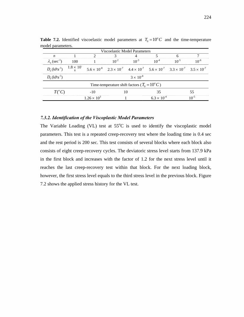
224
Table 7.2. Identified viscoelastic model parameters at and the time-temperature model parameters.
Viscoelastic Model Parameters 1 2 3 4 5 6 7
(sec-1) 100 1 10-2 10-3 10-4 10-5 10-6
(kPa-1) 1.8 10-
8 5.6 10-8 2.3 10-7 4.4 10-7 5.6 10-7 3.3 10-7 3.5 10-7
(kPa-1) 3 10-8
Time-temperature shift factors ( )
-10 10 35 55
1.26 103 1 6.3 10-4 10-5
7.3.2. Identification of the Viscoplastic Model Parameters
The Variable Loading (VL) test at 55oC is used to identify the viscoplastic model
parameters. This test is a repeated creep-recovery test where the loading time is 0.4 sec
and the rest period is 200 sec. This test consists of several blocks where each block also
consists of eight creep-recovery cycles. The deviatoric stress level starts from 137.9 kPa
in the first block and increases with the factor of 1.2 for the next stress level until it
reaches the last creep-recovery test within that block. For the next loading block,
however, the first stress level equals to the third stress level in the previous block. Figure
7.2 shows the applied stress history for the VL test.
0 10oT C
n
n
nD
0D
0 10oT C
( )oT C

225
(a)
(b)
Figure 7.1. Complex modulus data in compression at different temperatures; (a) before time-temperature shift; (b) after time-temperature shift.
-8
-7.5
-7
-6.5
-6
-5.5
-5
-4.5
-1.5 -0.5 0.5 1.5 2.5
Log
(D*)
[kP
a-1]
Log(Angular frequency) [Rad/Sec]
T=-10C
T=10C
T=35C
T=55C
-8
-7.5
-7
-6.5
-6
-5.5
-5
-4.5
-8 -6 -4 -2 0 2 4 6
Log
(D*)
[kP
a-1]
Log(Reduced angular frequency) [Rad/Sec]
T=-10C Shifted
T=10C Shifted
T=35C Shifted
T=55C Shifted

226
Figure 7.2. Stress history for the Variable Loading (VL) test.
Once the viscoelastic model parameters are identified, the viscoelastic and
viscoplastic strain responses can be separated. The separated viscoplastic strain
responses for the initial loading cycles are used to identify the viscoplastic model
parameters (please refer to Chapter II and Huang et al. (2011) for more details on
identification of the viscoplastic model parameters). It should be noted that the
viscoplastic model parameters are identified at 55oC, whereas, the viscoelastic model
parameters are identified at 10oC. Therefore, it is assumed primarily that the time-
temperature shift factors are the same for the viscoelastic and viscoplastic responses.
Having this assumption in hand, the identified viscoplastic model parameters are shifted
to the reference temperature (i.e. 10oT C ) using the same time-temperature shift factor
identified from the dynamic modulus test. This can be achieved by simply scaling the
viscoplasticity viscosity parameter vp [i.e. 010 55 55, 10vp o vp o oTC C a T C ].
This simple analysis allows one to use the same time-temperature shift factor for
viscoelasticity and viscoplasticity and avoids the confusion. The rest of the viscoplastic
model parameters remain the same for both temperatures. Table 7.3 lists the viscoplastic
model parameters at reference temperature (i.e. ).
0
200
400
600
800
1000
1200
1 5 9 13 17 21
Stre
ss L
evel
(kP
a)
Loading Cycle (N)
10oT C

227
Table 7.3. Viscoplastic model parameters at the reference temperature 0 10oT C . (Note that these parameters are obtained using the viscoplastic parameters identified at 55oC and the time-temperature shift factor identified from dynamic modulus test).
0y (kPa)
vp (sec-1) N 0 (kPa) 1 (kPa) 2
0.25 0.2 100 2.4 10-8 1.0 50 1800 135
Figure 7.3 shows the comparison between the experimental data and model
predictions for the VL test at 55oC. Figure 7.3 shows that model predictions agree well
with the experimental data within the first block.
Figure 7.3. Model predictions and experimental measurements for the VL test at 55oC.
However, the model does not show more viscoplastic strain in the second block
until the applied stress level exceeds its maximum value in the previous block. However,
experimental measurements show that asphalt mixes progressively accumulate the
permanent deformation even when the applied stress is less than its maximum value in
the previous block (more viscoplastic strain is accumulated for the first four loading
cycles in the second block even though the applied stress is still less than the applied
stress at the end of the first block).
0
0.1
0.2
0.3
0.4
0.5
0 500 1000 1500 2000 2500 3000 3500
Stra
in (%
)
Time (sec)
Experimental measurements
Model prediction using VE-VP model

228
This distinct behavior of asphalt mixes subjected to the repeated loading at high
temperatures cannot be explained by hardening plasticity and viscoplasticity theories
only. In other words, the hardening plasticity/viscoplasticity theories state that the
material point remains inside the yield surface (i.e. elastic/viscoelastic) when the applied
stress in the subsequent loading cycle is less than the stress level in the preceding
loading cycle such that no further permanent deformation is predicted. However, as it is
obvious from Figure 7.3, asphalt mixes once yielded show accumulation of the
plastic/viscoplastic strain in each loading cycle even if the applied stress is decreasing.
Although this behavior can be explained by the viscodamage model, it is not physical to
relate this degradation behavior to the damage model since at this high temperature and
in compression loading conditions the material rarely experiences micro-cracking. This
behavior is related in this work to the viscoplastic softening which will be explained in
more details in the next subsection.
7.3.3. Viscoplastic Softening Model and the Viscoplastic Softening Memory Surface
Asphalt mixes are subjected to repeated loading during their service life. The
microstructure of the asphalt mixes rearranges during the unloading and rest period
especially at high temperatures. This rearrangement of the microstructure (i.e.
rearragement of the aggregates) changes the mechanical properties of the asphalt mixes
such that they can undergo more viscoplastic deformation during the next loading cycle.
This behavior is referred to as the viscoplastic softening, (Saadeh et al., 2007). There are
several approaches to model the viscoplastic softening in materials. The first approach is
to allow the yield surface to shrink during the unloading to take into account the
softening behavior. This approach has been used by Yum and Kim (2011) to predict the
viscoplastic softening response of asphalt mixes at high temperatures. However, their
model is augmented with more than seven model parameters which increase the number
of required tests to identify the parameters. The second approach is to additively
decompose the hardening/softening function in the viscoplastic dynamic yield surface
into hardening and softening components, such that:
h s (7.3)

229
where h and s are hardening and softening components of the function ,
respectively. The hardening and softening components can then be obtained by
proposing certain evolution functions. The third approach is to consider the viscoplastic
softening effect through the maximum saturation limit of the viscoplastic hardening
function. In other words, the classical plasticity/viscoplasticity theories state that the
isotropic hardening saturates for large values of the viscoplastic strains. However, if
unloading occurs after the saturation point of the isotropic hardening, additional
softening is observed again which causes the evolution of more plastic/viscoplastic strain
under the same stress level. Therefore, the saturation limit of the isotropic hardening is
not constant and changes during the unloading which is accompanied with the changes
in the microstructure. For example, the saturation limit of the viscoplastic model used in
this work is 0 1 . In this approach, one can express the parameter 1 to be a
decreasing function of the effective viscoplastic strain from previous loading cycles.
However, numerous other conditions should also be used in these approaches.
For example, the experimental measurements show that the softening occurs when the
viscoplastic strain exceeds a certain value. Therefore, one should put another condition
to capture this effect in order to avoid overestimation of the viscoplastic softening.
Moreover, experimental measurements usually show the presence of a lower limit for the
viscoplastic softening such that the material cannot get softer than that limit. Again,
another condition is required to capture this effect. More importantly, these models are
usually developed for specific loading conditions and should be used with special cares
for the general cases.
The last approach and the most robust approach, in the author’s opinion, is to
define a surface in the viscoplastic strain space instead of the stress space as the
viscoplastic softening memory surface. The memory surface can be considered as the
counterpart of the yield surface in the viscoplastic strain space. This surface can be
expressed in terms of an internal state variable which memorizes the maximum
experienced viscoplastic strain in the last unloading stage. The evolution of the
viscoplastic softening will then be controlled by this surface. This concept has been used

230
for a different purpose in modeling the stabilization of the hysteresis loops in cyclic
plasticity of metals (Murakami and Ohno, 1982; Ohno, 1982; Chaboche, 1989).
Analogously, in this study the static viscoplastic memory surface can be defined as
follows:
,soft 0vp vpf p q (7.4)
where ,softvpf is the static viscoplastic memory surface, p is the effective viscoplastic
strain, and vpq is the viscoplastic internal state variable memorizing the maximum
experienced viscoplastic strain for which the softening has occurred. Eq. (7.4) shows that
the material does not undergo viscoplastic softening if ,soft 0vpf . However, similar to
the rate-dependent plasticity (i.e. viscoplasticity), the value of the static viscoplastic
softening memory surface can have a positive value if the viscoplastic strain exceeds the
viscoplastic softening internal state variable. The distance of the viscoplastic strain from
the static viscoplastic softening memory surface controls the rate of the evolution of the
viscoplastic softening internal state variable, such that one can define a dynamic
viscoplastic softening memory surface as follows:
1
1
,soft,soft
0vp S
vp vpvp
qp q
(7.5)
where ,softvp is the dynamic viscoplastic softening memory surface, ,softvp is the
viscoplastic softening viscosity parameter, and 1S is a model parameter. The rate of the
evolution of the viscoplastic softening internal state variable vpq can be determined
based on Eq. (7.5), such that:
1,soft Svp vp vpq p q (7.6)
This equation clearly shows that the rate of the viscoplastic softening internal state
variable depends on the difference of the effective viscoplastic strain and the maximum
value of the viscoplastic strain for which the softening has occurred. In other words,
vpp q is the amount of the viscoplastic strain for which the material has not yet
rearranged its microstructure during the unloading (i.e. viscoplastic softening has not

231
occurred for this deformation). In fact, this difference is the driving force for the
viscoplastic softening. Now, as the first try, one can assume that the evolution function
for the saturation limit of the hardening parameter 1 to be a linear function of the
viscoplastic softening internal state variable, such that:
1 2vpS q (7.7)
However, Eq. (7.7) is modified as follows to consider the history effect in the
viscoplastic softening model since the experimental measurements show that the rate of
the viscoplastic softening decreases as the saturation limit of the hardening parameter
decreases, such that:
3
11 2 initial
1
S
vpS q
(7.8)
Figure 7.4 shows the schematic representation of the concept of the viscoplastic
softening memory surface.
Figure 7.4. Schematic representation of the concept of the viscoplastic softening memory surface.
Static viscoplastic softening memory surface
Determines rate of the viscoplastic softening internal state variable
Dynamic viscoplastic softening memory surface
p
vpq
1vp
2vp3
vp

232
This approach provides a promising framework for modeling the viscoplastic
softening mechanism in the materials. This dynamic viscoplastic softening memory
surface distinguishs between the viscoplastic softening under extension and compressive
loading conditions. The identification of the model parameters is pretty straightforward
and is similar to identification of the parameters associated with the yield surface in the
stress space. Therefore, one can easily conduct repeated creep-recovery tests at high
temperatures and for different loading/unloading times to identify the model parameters.
Alternatively, one can use the flow test to identify the viscoplastic softening model
parameters. The identified model parameters associated with the ALF materials at 55oC
are listed in Table 7.4.
Table 7.4. Identified viscoplastic softening model parameters. ,softvp (sec-1) 1S 2S (kPa) 3S
0.001 0.3 200000 2.5
The variable loading test is resimulated using the viscoplastic softening memory
surface as shown in Figure 7.5. As shown in Figure 7.5 (a), inclusion of the viscoplastic
softening model through the viscoplastic softening memory surface significantly
enhances the model prediction of the strain response in the VL test. Moreover, the
evolution of the saturation limit of the viscoplastic model (i.e. 1 ) with time is plotted in
Figure 7.5 (b). This Figure shows that the material undergoes softening during the rest
period. However, the viscoplastic model parameters are identified such that the softening
continues until the rate of the viscoplastic strain reaches a negligible value. After that
point, no softening occurs since the softening is physically related to the rearrangement
of the microstructure during the unloading. Therefore, no more softening is expected
once the rate of the recoverable strain in the unloading reaches zero.

233
(a)
(b)
Figure 7.5. Experimental measurements and model prediction with and without viscoplastic memory surface for the variable loading test (VL) at 55oC in compression. (a) strain response;
(b) evolution of the parameter with time.
0
0.1
0.2
0.3
0.4
0.5
0 500 1000 1500 2000 2500 3000 3500
Stra
in (%
)
Time (sec)
Experimental measurements
Model prediction without memory surface
Model prediction with memory surface
0
600
1200
1800
0 500 1000 1500 2000 2500 3000 3500
k 1(k
Pa)
Time (sec)
1

234
7.4. Model Validation in Compression
The calibrated VE-VP model along with the viscoplastic softening model are used to
further validate the model against the experimental data listed in Table 7.5 which has not
been used in the calibration process.
Table 7.5. Summary of the test used for validation of the viscoelastic-viscoplastic model with viscoplastic softening model*
Test Stress level
(kPa) Loading time
(Sec) Rest period (Sec)
Repeated creep-recovery test with constant loading level and time (CLT)
827 0.1, 0.4, 1.6, 6.4 0.9
Repeated creep-recovery test with variable loading time (VT)
827 Sequence of (0.05, 0.1, 0.4, 1.6, 6.4)
0.05, 1, 200
Repeated creep-recovery test with reversed variable loading time (RVT)
827 Sequence of (6.4, 1.6, 0.4, 0.1, 0.05)
200
* All tests have done at 55oC and 140kPa confinement in compression
7.4.1. Model Validation against Constant Loading Time Test (CLT)
Figure 7.6 schematically shows the stress history input for CLT.
Figure 7.6. Schematic representation of the stress input for the constant loading time test (CLT). NCSU database includes CLT tests for four different loading times (LT) of 0.1, 0.4, 1.6, and 6.4
sec.
……..
Time (sec)
Deviatoric stress (kPa)
827 (kPa)
LT UT=0.9sec

235
The constant loading time test (CLT) is basically a simple repeated creep-
recovery test with the rest periods between the loading cycles. The applied stress level,
loading time, and rest period are kept constant for each test. However, this test is
repeated for four loading times of 0.1, 0.4, 1.6, and 6.4 sec. The rest period in all these
four tests equals to 0.9 sec. The applied deviatoric stress is also constant for these four
tests and equals to 827 kPa. Figures 7.7 and 7.8 show the comparison of the model
prediction with and without the memory surface with the experimental measurements
when the loading times are 0.1 and 0.4sec, respectively. As shown in Figures 7.7(a) and
7.8(a), the VE-VP model shows that the viscoplastic strain saturates after the first one or
two loading cycle. Therefore, it predicts no more viscoplastic strain for the next loading
cycles. However, experimental measurements and model predictions with memory
surface clearly show that the material can undergo more viscoplastic strain after the
unloading occurs. This phenomenon can be clearly seen in Figures 7.7(b) and 7.8(b).
These figures show that the material softens during the unloading by decreasing the
saturation limit of the hardening function 1 . However, the rate of softening decreases as
the viscoplastic strain increases and as the hardening parameter 1 decreases. This
behavior is related to the inclusion of the history term 3
1initial1
S
in Eq. (7.8). This
history term slows the rate of the viscoplastic softening as the hardening parameter 1
decreases. Figures 7.7 and 7.8 show that the model with the viscoplastic memory surface
agrees well with the experimental measurements. Model predictions and experimental
measurements for longer loading times of 1.6sec and 6.4sec are presented in Figure 7.9.
Figure 7.9 shows that as the loading time increases, the viscoplastic softening model
slightly overestimates the experimental measurements. It should be noted that loading
times 1.6 and 6.4sec resemble very high vehicle speed which are less likely to happen in
the roads and pavements. However, more experimental data is required to investigate the
reason for this overestimation as the loading time increases.

236
(a)
(b)
Figure 7.7. Experimental measurements and model prediction with and without viscoplastic memory surface for the constant loading and time test (CLT) at 55oC in compression when the
loading time is 0.1sec. (a) strain response; (b) evolution of the parameter with time.
0.0
0.2
0.4
0.6
0.8
1.0
1.2
0 200 400 600 800 1000
Stra
in (%
)
Time (Sec)
Experimental measurements
Model prediction without memory surface
Model prediction with memory surface
0
600
1200
1800
0 200 400 600 800 1000
k 1(k
Pa)
Time (Sec)
1

237
(a)
(b)
Figure 7.8. Experimental measurements and model prediction with and without viscoplastic memory surface for the constant loading and time test (CLT) at 55oC in compression when the
loading time is 0.4 sec. (a) strain response; (b) evolution of the parameter with time.
0.0
0.2
0.4
0.6
0.8
1.0
1.2
0 100 200 300 400 500
Str
ain
(%)
Time (Sec)
Experimental measurements
Model prediction without memory surface
Model predictions with memory surface
0
600
1200
1800
0 100 200 300 400 500
k 1(k
Pa)
Time (Sec)
1

238
(a)
(b)
Figure 7.9. Experimental measurements and model prediction with and without viscoplastic memory surface for the constant loading and time test (CLT) at 55oC in compression. (a) loading
time is 1.6sec; (b) loading time is 6.4sec.
0.0
0.2
0.4
0.6
0.8
1.0
1.2
1.4
0 200 400 600 800 1000
Stra
in (%
)
Time (Sec)
Experimental measurements
Model prediction without memory surface
Model prediction with memory surface
0.0
0.2
0.4
0.6
0.8
1.0
1.2
1.4
0 200 400 600 800 1000 1200 1400
Stra
in (%
)
Time (Sec)
Experimental measurements
Model prediction without memory surface
Model prediction with memory surface

239
7.4.2. Model Validation against Variable Loading Time Test (VT)
Variable loading time test (VT) is a repeated creep-recovery test where the applied
deviatoric stress and the rest period between the loading cycles are kept constant and
equal to 827kPa and 200sec, respectively. This test is designed to investigate the effect
of loading time on mechanical response of asphalt mixes. VT consists of several blocks
with each block consisting of six creep-recovery tests. The loading time in each block
varies from short to long loading times with the sequence of 0.05, 0.1, 0.2, 0.4, 1.6, and
6.4 sec. The schematic representation of the stress input in VT test is shown in Figure
7.10. The unloading time (UT) remains constant during each test. However, the VT test
is conducted at three different unloading times (i.e. rest periods) of 0.05, 1, and 200 sec
to investigate the effect of the rest period as well.
Figure 7.10. Schematic representation of stress input in variable loading time test (VT). The
unloading time (UT) is constant and equals to 200 sec.
Figures 7.11 (a), (b), and (c) show the model predictions and experimental
measurements for the variable loading time test when the rest periods are 0.05, 1, and
200 sec, respectively.
……..
Time (sec)
Deviatoric stress (kPa)
827 (kPa)
0.05
UT
0.1 0.2 0.4 1.6 6.4
Block 1

240
(a)
(b)
Figure 7.11. Experimental measurements and model prediction with and without viscoplastic memory surface for the variable loading time test (VT) at 55oC in compression. (a) rest period is
0.05sec; (b) rest period is 1sec; (c) rest period is 200sec.
0
0.2
0.4
0.6
0.8
1
1.2
1.4
0 50 100 150 200 250 300 350
Stra
in (%
)
Time (Sec)
Experimental measurements
Model prediction without memory surface
Model prediction with memory surface
0.0
0.2
0.4
0.6
0.8
1.0
1.2
1.4
1.6
0 50 100 150 200 250 300 350 400
Stra
in (%
)
Time (Sec)
Experimental measurements
Model prediction without memory surface
Model prediction with memory surface

241
(c)
Figure 7.11. Continued.
7.4.3. Model Validation against Reversed Variable Loading Time Test (RVT)
Figure 7.12 shows the schematic representation of the stress history for the reversed
variable loading time test.
Figure 7.12. Schematic representation of stress input in the reversed various loading time test (RVT). The unloading time (UT) is constant and equals to 200 sec.
0
0.2
0.4
0.6
0.8
1
1.2
0 1000 2000 3000 4000 5000 6000
Stra
in (%
)
Time (sec)
Experimental measurements
Model prediction without memory surface
Model prediction with memory surface
……..
Time (sec)
Deviatoric stress (kPa)
827 (kPa) UT
0.05 0.1 0.2 0.4 1.6 6.4
Block 1

242
Reversed variable loading time test (RVT) is very similar to the variable loading
time test (VT) with the difference that the loading time in each block starts from its
maximum value and decreases to its minimum value. The applied deviatoric stress is
kept constant and equal to 827kPa. However, the loading time is a sequence of 6.4, 1.6,
0.4, 0.2, 0.1, and 0.05sec. The unloading time or the rest period in this test is constant
and is equal to 200sec. Figure 7.13 shows the model predictions and experimental
measurements for the reversed variable loading time test. Figure 7.13 shows that the
model prediction without the viscoplastic memory surface significantly underestimates
the experimental measurements while the model prediction with the viscoplastic
memory surface overestimates the experimental measurements.
Figure 7.13. Experimental measurements and model prediction with and without viscoplastic
memory surface for the reversed variable loading time test (RVT) at 55oC in compression.
7.5. Effect of Viscoplastic Softening Model on the Mechanical Response
The effect of different model parameters associated with the viscoplastic softening
memory surface and the evolution function for the saturation hardening parameter 1 is
investigated in this section. The first block of the CLT test with 0.1sec loading time and
0.0
0.2
0.4
0.6
0.8
1.0
1.2
1.4
1.6
0 1000 2000 3000 4000 5000 6000 7000
Stra
in (%
)
Time (Sec)
Experimental measurements
Model prediction without memory surface
Model prediction with memory surface

243
0.9sec unloading time is selected to investigate this issue. Figure 7.14 shows the effect of
the viscoplasticity softening viscosity parameter ,softvp on the evolution of the
viscoplasticity softening internal variable vpq . As shown in Figure 7.14, the viscoplastic
softening viscosity parameter controls the rate of the change in the viscoplastic internal
state variable vpq . For example, Figure 7.14 shows that when , 0.1vp soft sec-1, the
material can fulfill its full softening potential during the rest period of 0.9sec. However,
the material can only partially fulfill its softening potential when , 0.001vp soft sec-1.
However, the material will fulfill its full softening potential once a long enough rest
period is introduced. Figure 7.14 shows an interesting feature of the model in capturing
time-dependent viscoplastic softening response. It is noteworthy that the difference
between the effective viscoplastic strain p and the viscoplastic softening internal state
variable vpq is the driving force for the viscoplastic softening.
Figure 7.14. Effect of the viscoplastic softening viscosity parameter ,softvp on the evolution of
the viscoplastic softening internal state variable vpq . The other parameters are selected as :
1 0.3S and 2 0S .
0
0.05
0.1
0.15
0.2
0.25
0.3
0 1 2 3 4 5
Vis
copl
asti
c so
ften
ing
inte
rnal
var
iabl
e
Time (sec)
, 0.1/secvp soft , 0.01 / secvp soft
, 0.001/secvp soft
p

244
The value of ,soft 0.001vp sec-1 is selected to investigate the effect of the rate-
sensitivity parameter 1S on the evolution of the viscoplastic softening internal state
variable. Figure 7.15 shows that the 1S parameter also controls the rate of change in the
viscoplastic softening internal state variable. Comparing Figures 7.14 and 7.15 shows
that the parameter ,softvp changes both the value and the shape of the curve for the
viscoplastic softening state variable, whereas, parameter 1S only affects the rate of the
change in the viscoplastic internal state variable.
Furthermore, Figures 7.16(a) and 7.16(b) show the effect of and
parameters on the softening response of materials.
Figure 7.15. Effect of the viscoplastic softening parameter 1S on the evolution of the
viscoplastic softening internal state variable vpq . The other parameters are selected as :,soft 0.001 / secvp and 2 0S .
2S 3S
0
0.05
0.1
0.15
0.2
0 1 2 3 4
Vis
copl
asti
c so
ften
ing
inte
rnal
var
iabl
e
Time (sec)
S1=0.1
S1=0.3
S1=0.5
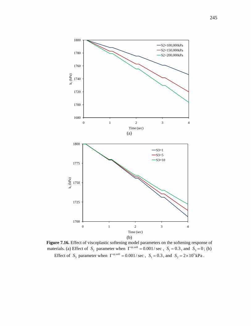
245
(a)
(b)
Figure 7.16. Effect of viscoplastic softening model parameters on the softening response of materials. (a) Effect of parameter when , , and ; (b)
Effect of parameter when , , and .
1680
1700
1720
1740
1760
1780
1800
0 1 2 3 4
k 1(k
Pa)
Time (sec)
S2=100,000kPa
S2=150,000kPa
S2=200,000kPa
1700
1725
1750
1775
1800
0 1 2 3 4
k 1(k
Pa)
Time (sec)
S3=1
S3=5
S3=10
2S ,soft 0.001 / secvp 1 0.3S 3 0S
3S ,soft 0.001 / secvp 1 0.3S 52 2 10 kPaS

246
Figure 7.16(a) shows that the softening viscoplastic response signifies as the
parameter 2S increases. However, the history model parameter 3S controls the rate of
the viscoplastic softening as the material softens.
7.6. Identification of the Model Parameters in Tension
The NCSU test data in tension include complex modulus, uniaxial constant strain rate,
cyclic stress control, and cyclic strain control tests at different temperatures, strain rates,
strain levels, and stress levels. The monotonic uniaxial constant strain rates at 5oC are
used to calibrate the damage model, whereas, the other test data are used to further
validate the model presented in Chapter II. Tables 7.6 and 7.7 list the tests which have
been used to calibrate and validate the model respectively.
Table 7.6. Summary of the tests in tension used for identification of the thermo-viscodamage model parameters.
Test Temperature ( o C ) Strain rate (sec-1) Uniaxial constant strain rate test 5 7 10-6; 2.1 10-5; 3 10-5; 5.5 10-5
Table 7.7. Summary of the tests in tension used for validation of the thermo-viscoelastic-viscoplastic-viscodamage-model.
Test Temperature (
o C ) Stress level
(kPa) Strain level
( ) Strain rate (sec-1)
Complex Modulus test -10, 10, 35, 55
Uniaxial constant strain arte test
12 2.7 10-4; 4.6 10-4
25 5 10-4; 1.5 10-3;
4.5 10-3; 1.35 10-2
40 3 10-4; 10-3;
3 10-3
Cyclic stress control 5 1525
19 250, 750
Cyclic strain control 5 1750
19 1200, 1500

247
7.6.1. Viscoelastic-Viscoplastic Parameters in Tension and Time-Temperature Shift
Factors
The NCSU database includes the dynamic modulus tests in both tension and
compression for the same temperatures and frequencies (i.e. -10, 10, 35, and 55oC; and
0.01, 0.05, 0.1, 0.5, 1, 5, 10, and 25 Hz). It is usually argued that the viscoelastic
response of asphalt mixes is controlled by the viscoelastic response of the asphalt binder.
However, the viscoelastic response of asphalt binder is practically the same in tension
and compression. Therefore, the viscoelastic response of asphalt mixes should also be
similar in tension and compression. To investigate this issue, the complex modulus data
at different temperatures are plotted versus the angular frequency for both tension
and compression in Figure 7.17 (a). Figure 7.17 (a) shows that the viscoelastic response
of asphalt mixes is the same in both tension and compression for a range of temperatures
(i.e. -10oC-35oC).
However, the viscoelastic response in tension and compression deviate from each
other as the temperature increases. Moreover, this deviation signifies at low angular
frequencies. The reason is that asphalt mixes at high temperatures are very prone to
viscoplastic deformation and cracking in compression and tension, respectively.
Therefore, the measured complex compliance at high temperatures includes viscoplastic
response in compression and damage response in tension. Furthermore, at low angular
frequencies, the applied load remains on the specimen for a longer time which signifies
the effect of the viscoplastic evolution and damage evolution in compression and
tension, respectively. However, surprisingly the time-temperature shift factors in both
tension and compression are the same. Figure 7.17 (b) shows the shifted complex
compliance data to the reference temperature using the same time-
temperature shift factor listed in Table 7.2. Therefore, for the range of the temperatures
for which the tension data are available (i.e. 5-25oC) the same viscoelastic parameters
and time-temperature shift factors identified in compression can be used. Moreover,
is used to differentiate between the viscoplastic response in tension and
compression.
0 10oT C
0.78vpd

248
(a)
(b)
Figure 7.17. The complex compliance data at different temperatures. (a) before time-temperature shift factor; (b) after time-temperature shift.
7.6.2. Viscodamage Model Parameters in Tension
The constant uniaxial strain rate tests in tension at 5oC are analyzed to identify the
viscodamage model parameters. At this temperature, one can assume reasonably that the
material is only viscoelastic since the viscoplastic response can be reasonably neglected
-8
-7.5
-7
-6.5
-6
-5.5
-5
-4.5
-1.5 -0.5 0.5 1.5 2.5
Log
(D*)
[kP
a-1]
Log(Angular frequency) [Rad/Sec]
T=-10C, TensionT=10C, TensionT=35C, TensionT=55C, TensionT=-10C, CompressionT=10C, CompressionT=35C, CompressionT=55C, Compression
-8
-7.5
-7
-6.5
-6
-5.5
-5
-4.5
-8 -6 -4 -2 0 2 4 6
Log
(D*)
[kP
a-1]
Log(Reduced angular frequency) [Rad/Sec]
T=-10C Shifted, Tension
T=10C Shifted, Tension
T=35C Shifted, Tension
T=55C Shifted, Tension
T=-10C Shifted, Compression
T=10C Shifted, Compression
T=35C Shifted, Compression
T=55C Shifted, Compression

249
at low temperatures. To examine the accuracy of this assumption, the VE-VP model
parameters along with the time-temperature shift factors are used to simulate the
response of asphalt mixes at 5oC when the strain rate is 1 10-4/sec. Figure 7.18 shows
the predicted viscoplastic strain versus the total applied strain. Figure 7.18 shows that the
predicted viscoplastic strain is less than 1% of the total applied strain which reasonably
verifies the assumption of neglecting the viscoplastic strain at 5oC. Moreover, the
constant strain rate test is selected since one can analytically obtain the response in the
healing configuration and subsequently identify the damage variable.
Figure 7.18. Predicted viscoplastic strain versus the total applied strain at 5oC when the strain
rate is 1 10-4/sec. It shows that the viscoplastic strain can be reasonably neglected at 5oC.
To show the procedure, one can assume the strain input for the constant strain
rate test as follows:
t Ct (7.9)
where C is a constant representing the strain rate in the uniaxial constant strain rate
response. The uniaxial stress output in the healing configuration can be simply obtained
0
0.002
0.004
0.006
0.008
0.01
0.012
0 0.2 0.4 0.6 0.8 1
Vis
copl
asti
c st
rain
(%)
Total strain (%)
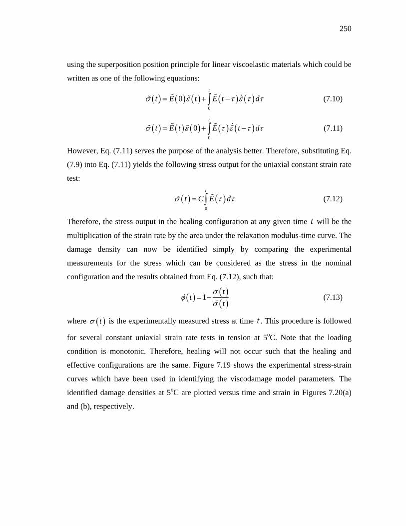
250
using the superposition position principle for linear viscoelastic materials which could be
written as one of the following equations:
0
0t
t E t E t d (7.10)
0
0t
t E t E t d (7.11)
However, Eq. (7.11) serves the purpose of the analysis better. Therefore, substituting Eq.
(7.9) into Eq. (7.11) yields the following stress output for the uniaxial constant strain rate
test:
0
t
t C E d (7.12)
Therefore, the stress output in the healing configuration at any given time t will be the
multiplication of the strain rate by the area under the relaxation modulus-time curve. The
damage density can now be identified simply by comparing the experimental
measurements for the stress which can be considered as the stress in the nominal
configuration and the results obtained from Eq. (7.12), such that:
1t
tt
(7.13)
where t is the experimentally measured stress at time t . This procedure is followed
for several constant uniaxial strain rate tests in tension at 5oC. Note that the loading
condition is monotonic. Therefore, healing will not occur such that the healing and
effective configurations are the same. Figure 7.19 shows the experimental stress-strain
curves which have been used in identifying the viscodamage model parameters. The
identified damage densities at 5oC are plotted versus time and strain in Figures 7.20(a)
and (b), respectively.

251
Figure 7.19. Stress-strain curves at 5oC which have been used in identifying the viscodamage
model parameters.
Now, let one assume the following form for the rate of the damage density as a
function of the normalized effective damage force and strain:
(7.14)
where is the damage force at the reference stress level which could be selected
arbitrary.
Taking the natural logarithm of both sides implies:
(7.15)
0
1000
2000
3000
4000
5000
0 0.1 0.2 0.3 0.4 0.5 0.6 0.7 0.8
Stre
ss (k
Pa)
Strain (%)
Strain rate=7E-6/sec
Strain rate=2.1E-5/sec
Strain rate=3E-5/sec
Strain rate=5.5E-5/sec
1 20
vd Yf f
Y
0Y
1 20
vd YLn Ln Ln f Ln f
Y

252
(a)
(b)
Figure 7.20. The identified damage density versus time and strain for different constant strain
rate tests at 5oC.
Now, as shown in Figure 7.21, one can simply plot the rate of the damage density versus
strain using experimental measurements.
0
0.2
0.4
0.6
0.8
1
0 100 200 300 400 500 600 700 800
Dam
age
dens
ity
Time (sec)
Strain rate=7.00E-6/sec
Strain rate=2.10E-5/sec
Strain rate=3.00E-5/sec
Strain rate=5.50E-5/sec
0
0.2
0.4
0.6
0.8
1
0 0.1 0.2 0.3 0.4 0.5 0.6 0.7
Dam
age
dens
ity
Strain (%)
Strain rate=7.00E-6/sec
Strain rate=2.10E-5/sec
Strain rate=3.00E-5/sec
Strain rate=5.50E-5/sec
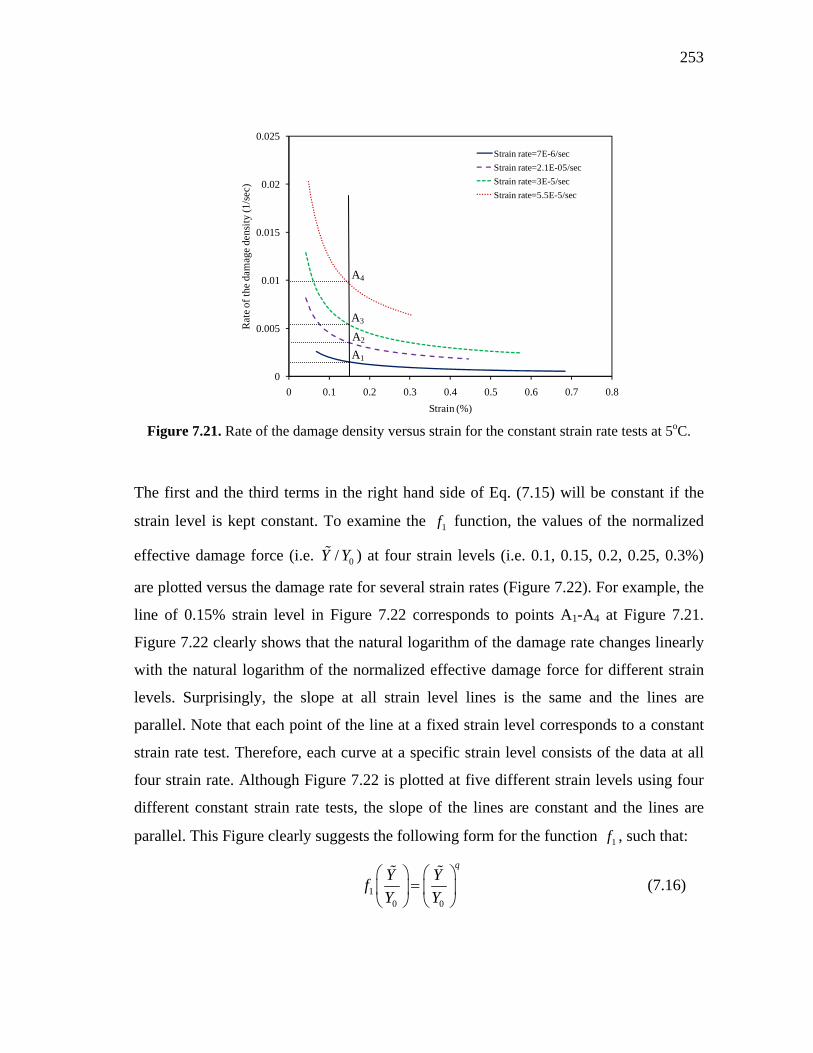
253
Figure 7.21. Rate of the damage density versus strain for the constant strain rate tests at 5oC.
The first and the third terms in the right hand side of Eq. (7.15) will be constant if the
strain level is kept constant. To examine the 1f function, the values of the normalized
effective damage force (i.e. 0/Y Y ) at four strain levels (i.e. 0.1, 0.15, 0.2, 0.25, 0.3%)
are plotted versus the damage rate for several strain rates (Figure 7.22). For example, the
line of 0.15% strain level in Figure 7.22 corresponds to points A1-A4 at Figure 7.21.
Figure 7.22 clearly shows that the natural logarithm of the damage rate changes linearly
with the natural logarithm of the normalized effective damage force for different strain
levels. Surprisingly, the slope at all strain level lines is the same and the lines are
parallel. Note that each point of the line at a fixed strain level corresponds to a constant
strain rate test. Therefore, each curve at a specific strain level consists of the data at all
four strain rate. Although Figure 7.22 is plotted at five different strain levels using four
different constant strain rate tests, the slope of the lines are constant and the lines are
parallel. This Figure clearly suggests the following form for the function 1f , such that:
10 0
qY Y
fY Y
(7.16)
0
0.005
0.01
0.015
0.02
0.025
0 0.1 0.2 0.3 0.4 0.5 0.6 0.7 0.8
Rat
e of
the
dam
age
dens
ity
(1/s
ec)
Strain (%)
Strain rate=7E-6/sec
Strain rate=2.1E-05/sec
Strain rate=3E-5/sec
Strain rate=5.5E-5/sec
A2
A3
A4
A1

254
where q is the slope of the lines. Furthermore, the interception of each strain level line
with the Y-axis is the summation of the first and the third terms of the right hand side of
Eq. (7.15) at that strain level. Therefore, the term vdLn and subsequently the
parameter vd can be identified since the strain level at each strain level line is given.
Figure 7.22. Plot of the damage rate versus the normalized effective damage density for
identification of the parameters q and vd .
This procedure allows the identification of the parameter q independent of the
other viscodamage parameters.
Similarly, as shown in Figure 7.23, one can plot the rate of the damage density
versus the effective damage force using the experimental measurements and Eq. (7.12).
-7.5
-7
-6.5
-6
-5.5
-5
-4.5
-4
1 1.5 2 2.5 3
Ln[
Dam
age
rate
]
Ln[Effective damage force/Y0]
Strain level=0.10%
Strain level=0.15%
Strain level=0.20%
Strain level=0.25%
Strain level=0.30%
A2
A3
A4
A1

255
Figure 7.23. Rate of the damage density versus the effective damage force Y for constant strain
rate tests at 5oC.
The first and the second terms of the right side of Eq. (7.15) are constant if the
effective damage force is kept constant. Therefore, one can fix the effective stress, and
therefore the effective damage force, and plot the damage rate versus strain for the fixed
values of the damage force in order to specify the function 2f . This plot is presented in
Figure 7.24. The line of 3000kPa effective stress in Figure 7.24 corresponds to points
B1-B4 at Figure 7.23. Figure 7.24 also shows that the changes in the rate of the damage
density versus strain for constant effective stress are linear. Therefore, the function 2f
will have the following form with k being the slope of the lines in Figure 7.24.
2kf (7.17)
0
0.005
0.01
0.015
0.02
0.025
0 5000 10000 15000 20000
Rat
e of
the
dam
age
dens
ity
(1/s
ec)
Effective stress (kPa)
Strain rate=7E-6/sec
Strain rate=2.1E-05/sec
Strain rate=3E-5/sec
Strain rate=5.5E-5/sec
B2
B3
B4
B1
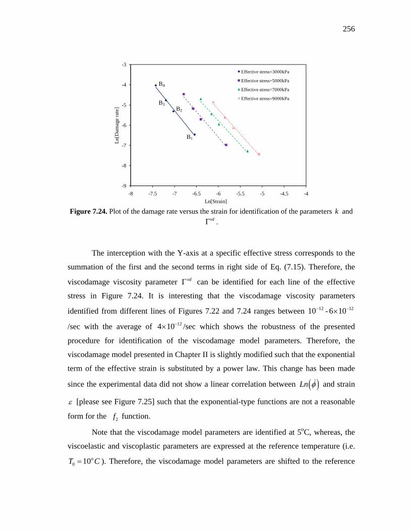
256
Figure 7.24. Plot of the damage rate versus the strain for identification of the parameters k and
vd .
The interception with the Y-axis at a specific effective stress corresponds to the
summation of the first and the second terms in right side of Eq. (7.15). Therefore, the
viscodamage viscosity parameter vd can be identified for each line of the effective
stress in Figure 7.24. It is interesting that the viscodamage viscosity parameters
identified from different lines of Figures 7.22 and 7.24 ranges between 1210 - 126 10
/sec with the average of 124 10 /sec which shows the robustness of the presented
procedure for identification of the viscodamage model parameters. Therefore, the
viscodamage model presented in Chapter II is slightly modified such that the exponential
term of the effective strain is substituted by a power law. This change has been made
since the experimental data did not show a linear correlation between Ln and strain
[please see Figure 7.25] such that the exponential-type functions are not a reasonable
form for the 2f function.
Note that the viscodamage model parameters are identified at 5oC, whereas, the
viscoelastic and viscoplastic parameters are expressed at the reference temperature (i.e.
0 10oT C ). Therefore, the viscodamage model parameters are shifted to the reference
-9
-8
-7
-6
-5
-4
-3
-8 -7.5 -7 -6.5 -6 -5.5 -5 -4.5 -4
Ln[
Dam
age
rate
]
Ln[Strain]
Effective stress=3000kPa
Effective stress=5000kPa
Effective stress=7000kPa
Effective stress=9000kPa
B2
B3
B4
B1

257
temperature using the same time-temperature shift factor identified from the dynamic
complex compliance test by scaling the viscodamage viscosity parameter such that
010 5 5, 10vd o vd o oTC C a T C . The assumption for this conversion is that the
same time-temperature shift factor can also be used for the damage model. This issue
will be investigated with more details in the following subsections. The viscodamage
model parameters at the reference temperature are listed in Table 7.8.
Figure 7.25. Plot of the natural logarithm of the damage rate versus strain for different strain rates at 5oC showing that the damage rate does not correlate with an exponential function of
strain.
Table 7.8. Viscodamage model parameters at the reference temperature 0 10oT C . (Note that these parameters are obtained using the viscodamage parameters identified at 5oC and the time-temperature shift factor identified from dynamic modulus test).
vd sec-1 0Y kPa q k
2.14 10-11 1000 2.41 -2.53
-9
-8
-7
-6
-5
-4
-3
0 0.1 0.2 0.3 0.4 0.5 0.6 0.7
Ln[
Dam
age
rate
]
Strain (%)
Effective stress=3000kPa
Effective stress=5000kPa
Effective stress=7000kPa
Effective stress=9000kPa

258
0
2000
4000
6000
8000
10000
12000
0 0.1 0.2 0.3 0.4 0.5 0.6 0.7 0.8
Stre
ss (k
Pa)
Strain (%)
Experimental measurements
Model prediction using VE-VP model
Model prediction using VE-VP-VD model
7.7. Validation of the Model against the Uniaxial Constant Strain Rate Tests in
Tension
The identified thermo-viscoelastic-viscoplastic-viscodamage model parameters are used
to validate the model against the constant strain rate tests at different temperatures and
strain rates. Figure 7.26 shows the model prediction and experimental measurements for
the constant strain rate tests at 5oC and at different strain rates. It should be noted that the
same time-temperature shift factor identified from the dynamic modulus test is used for
all components of the model (i.e. viscoelastic-viscoplastic-viscodamage). Figure 7.26
clearly shows that the model is capable of predicting the rate-dependent response of
asphalt mixes. It should be noted that the experimental measurements shown in Figure
7.26 have been used to identify and calibrate the viscodamage model parameters.
(a)
Figure 7.26. Model predictions and experimental measurements for the constant strain rate test in tension at 5oC when strain rates are: (a) 7 10-6/sec; (b) 2.1 10-5/sec; (c) 3 10-5/sec; (d) 5.5
10-5/sec.
0
3000
0 0.8

259
(b)
(c)
(d)
Figure 7.26. Continued.
0
5000
10000
15000
20000
0.00 0.10 0.20 0.30 0.40 0.50 0.60
Stre
ss (k
Pa)
Strain (%)
Experimental measurements
Model predictions using VE-VP model
Model prediction using VE-VP-VD model
0
2000
4000
6000
8000
10000
12000
0.00 0.10 0.20 0.30 0.40 0.50
Stre
ss (k
Pa)
Strain (%)
Experimental measurements
Model prediction using VE-VP model
Model prediction using VE-VP-VD model
0
2000
4000
6000
8000
10000
12000
14000
0.00 0.05 0.10 0.15 0.20 0.25 0.30 0.35
Stre
ss (k
Pa)
Strain (%)
Experimental measurements
Model prediction using VE-VP model
Model prediction using VE-VP-VD model
0
4000
0.0 0.6
0
4500
0.0 0.3
0
3500
0.0 0.5

260
Moreover, the model is also used to predict the response of the asphalt mixes
subjected to constant strain rate tests at 12oC, 25oC, and 40oC as well. Figure 7.27 shows
the model predictions and experimental measurements for two strain rates at 12oC.
Figures 7.27 (a) and (b) show that the model predictions agree well with the
experimental data when the damage is activated. The plots of the damage density versus
strain for the constant strain rate tests at 12oC are shown in Figure 7.28.
(a)
(b)
Figure 7.27. Model predictions and experimental measurements for the constant strain rate test in tension at 12oC when strain rates are: (a) 2.7 10-4/sec; (b) 4.6 10-4/sec.
0
2000
4000
6000
8000
10000
12000
14000
0.00 0.10 0.20 0.30 0.40 0.50
Stre
ss (k
Pa)
Strain (%)
Experimental measurements
Model prediction using VE-VP model
Model prediction using VE-VP-VD model
0
4000
8000
12000
16000
20000
0.00 0.10 0.20 0.30 0.40 0.50 0.60
Stre
ss (k
Pa)
Strain (%)
Experimental measurements
Model prediction using VE-VP model
Model prediction using VE-VP-VD model
0
3500
0.0 0.5
0
4000
0.0 0.6

261
Furthermore, Figure 7.29 shows further validation of the model at 25oC and for
four different strain rates. Also, Figure 7.30 shows the predicted damage density versus
strain for different strain rates at 25oC.
Figure 7.28. Predicted damage density versus strain for the constant strain rate test at 12oC.
(a)
Figure 7.29. Model predictions and experimental measurements for the constant strain rate test in tension at 25oC when strain rates are: (a) 5 10-4/sec; (b) 1.5 10-3/sec; (c) 4.5 10-3/sec; (d)
1.35 10-2/sec.
0.0
0.2
0.4
0.6
0.8
1.0
0.00 0.10 0.20 0.30 0.40 0.50
Dam
age
dens
ity
Strain (%)
0
1000
2000
3000
4000
5000
0.00 0.20 0.40 0.60 0.80 1.00 1.20
Stre
ss (k
Pa)
Strain (%)
Experimental measurements
Model prediction using VE-VP model
Model prediction using VE-VP-VD model
44.6 10 / sec
42.7 10 / sec
0
1500
0.0 1.2

262
(b)
(c)
(d)
Figure 7.29. Continued.
0
2000
4000
6000
8000
0.00 0.10 0.20 0.30 0.40 0.50 0.60 0.70 0.80
Stre
ss (k
Pa)
Strain (%)
Experimental measurements
Model prediction using VE-VP model
Model prediction using VE-VP-VD model
0
2000
4000
6000
8000
10000
12000
14000
0.00 0.20 0.40 0.60 0.80 1.00 1.20
Stre
ss (k
Pa)
Strain (%)
Experimental measurements
Model prediction using VE-VP model
Model prediction using VE-VP-VD model
0
5000
10000
15000
20000
25000
0.00 0.20 0.40 0.60 0.80
Stre
ss (k
Pa)
Strain (%)
Experimental measurements
Model predictions using VE-VP model
Model prediction using VE-VP-VD model
0
2000
0.0 0.8
0
3000
0.0 1.2
0
4500
0.0 0.8

263
Figure 7.30. Predicted damage density versus strain for the constant strain rate test at 25oC.
The model is further validated at 40oC for the constant strain rate test at several
strain rates. Figure 7.31 shows the model predictions and experimental measurements for
the stress-strain response at several strain rates. As it is shown in Figure 7.31 model
agrees well with the experimental data.
(a)
Figure 7.31. Model predictions and experimental measurements for the constant strain rate test
in tension at 40oC when strain rates are: (a) 3 10-4/sec; (b) 10-3/sec; (c) 3 10-3/sec.
0.0
0.2
0.4
0.6
0.8
1.0
0.00 0.10 0.20 0.30 0.40 0.50 0.60 0.70 0.80
Dam
age
dens
ity
Strain (%)
0
200
400
600
0.0 0.2 0.4 0.6 0.8
Stre
ss (k
Pa)
Strain (%)
Experimental measurements
Model prediction using VE-VP model
Model prediction using VE-VP-VD model
21.35 10 / sec
34.5 10 / sec
45 10 / sec
31.5 10 / sec
0
200
0.0 0.8

264
(b)
(c)
Figure 7.31. Continued.
Moreover, the damage density versus strain is plotted in Figure 7.32.
0
500
1000
0.0 0.2 0.4 0.6 0.8
Stre
ss (k
Pa)
Strain (%)
Experimental measurements
Model prediction using VE-VP model
Model prediction using VE-VP-VD model
0
500
1000
1500
0.0 0.2 0.4 0.6 0.8
Stre
ss (k
Pa)
Strain (%)
Experimental measurements
Model prediction using VE-VP model
Model prediction using VE-VP-VD model
0
300
0.0 0.8
0
500
0.0 0.8

265
Figure 7.32. Predicted damage density versus strain for the constant strain rate test at 40oC.
Figures 7.20, 7.28, 7.30, and 7.32 clearly show that the model predicts higher
damage value at fixed strain levels as the strain rate increases. This is in agreement with
experimental measurements on asphalt mixes. Predictions presented in this section
clearly shows that the proposed damage model is capable of predicting the rate- and
temperature response of asphalt mixes subjected to monotonic loading. Moreover, it is
usually recommended to identify the damage model parameters at low temperatures for
which the material is expected to undergo severe micro-cracking as the strain level
increases. The reason is that if the model can predict the severe damage condition, it
might also perform well at higher temperatures for which the rate of the damage growth
decreases.
The viscoelastic-viscoplastic-viscodamage model parameters along with the
time-temperature shift factors are also used to predict the response of the asphalt mixes
subjected to cyclic loading at 5 and 19oC. However, it should be mentioned that the
time-temperature shift factors for the damage model at 12oC, 19oC, 25oC, and 40oC are
assumed to be slightly different from the time-temperature shift factor identified from
the dynamic modulus test. However, this difference is negligible such that one can
consider the asphalt mix used in this study a thermo-rheological simple material for
0
0.2
0.4
0.6
0.8
1
0 0.1 0.2 0.3 0.4 0.5 0.6 0.7 0.8
Dam
age
dens
ity
Strain (%)
33 10 / sec
310 / sec
43 10 / sec

266
viscoelastic, viscoplastic, and viscodamage components. Figure 7.33 shows the
comparison between the time-temperature shift factors for the damage model and the
viscoelastic-viscoplastic model.
Figure 7.33. Comparison of the viscodamage time-temperature shift factor and the viscoelastic-
viscoplastic time-temperature shift factor (identified from dynamic modulus test) when the reference temperature is 10oC.
7.8. Validation of the Model against the Cyclic Stress Controlled Tests in Tension
The model is further validated against the cyclic stress controlled tests in tension. This
test is performed at 5oC and 19oC and for multiple stress amplitude. This test applies a
cyclic stress input with the frequency of 4cycles/sec, such that the stress input can be
written as follows:
max max cos 82 2
t (7.18)
where max is the stress amplitude. The schematic presentation of the stress history in
this test is shown in Figure 7.34. ft in Figure 7.34 can be considered as the failure time.
The number of loading cycles until which the material fails is therefore 4 ft .
-4
-3
-2
-1
0
1
0 10 20 30 40 50
Log
[Tim
e-te
mpe
ratu
re sh
ift f
acto
r]
T(oC)
VE-VP time-temperature shift factor
VD time-temperature shift factor

267
Figures 7.35(a) and (b) show the model predictions using viscoelastic-
viscoplastic model and the experimental measurements at initial loading cycles and
intermediate loading cycles for 750kPa stress amplitude, respectively. Figure 7.35(a)
shows that the model agrees reasonably well with experimental data for initial cycles.
However, as shown in Figure 7.35(b), model predictions deviates significantly from the
experimental data. This deviation should be compensated for with the viscodamage
model. As shown in Figure 7.36, the viscodamage component significantly enhances the
prediction of the cyclic response of asphalt mixes at large number of loading cycles.
Figure 7.34. Schematic representation of loading history for Controlled Stress cyclic test in tension.
Figure 7.37 shows the model predictions and experimental data of the strain
response for the cyclic stress control test at 19oC when the stress amplitude is 750kPa.
Time (sec)
(kPa)
0 0.5 1.0 tf-0.5 tf
max

268
(a)
(b)
Figure 7.35.Compasrison of the model prediction using viscoelastic-viscoplastic model and experimental data for the cyclic stress control test at 19oC when the stress amplitude is 750kPa.
(a) Loading cycles 1-30; (b) Loading cycles 970-980.
0
100
200
300
400
500
600
700
800
0.00 0.01 0.02 0.03 0.04 0.05
Stre
ss (k
Pa)
Strain (%)
Experimental data
Model prediction using VE-VP model
0
100
200
300
400
500
600
700
800
0.10 0.15 0.20 0.25 0.30 0.35
Stre
ss (k
Pa)
Strain (%)
Experimental data
Model prediction using VE-VP model

269
Figure 7.36. Comparison of the VE-VP-VD model prediction and experimental data for loading cycles 970-975 at 19oC when the stress amplitude is 750kPa.
Figure 7.37. Comparison of the experimental data and model predictions with and without
damage component for the strain response in the cyclic stress control test at 19oC when the stress amplitude is 750kPa.
0
100
200
300
400
500
600
700
800
0.28 0.29 0.30 0.31 0.32
Stre
ss (k
Pa)
Strain (%)
Experimental data
Model prediction using VE-VP-VD model
0.0
0.2
0.4
0.6
0.8
1.0
1.2
0 500 1000 1500 2000 2500 3000 3500 4000
Stra
in (%
)
Number of loading cycle (N)
Experimental measurements
Model prediction using VE-VP model
Model prediction using VE-VP-VD model

270
Moreover, Figure 7.38 shows model predictions and experimental measurements
for the same test and temperature when the stress amplitude is 250 kPa.
Figure 7.38. Comparison of the experimental data and model predictions with and without
damage component for the strain response in the cyclic stress control test at 19oC when the stress amplitude is 250kPa.
Figure 7.38 shows that the model prediction without damage saturates very fast
and significantly underestimates the experimental measurements. However, model
predictions agree reasonably well when the viscodamage component of the model is
activated. The NCSU database also includes the cyclic control stress test at 5oC when the
stress amplitude is 1525kPa. The identified model predictions along with the time-
temperature shift factors shown in Figure 7.33 are used to predict the strain response of
the cyclic control stress test at 5oC. As shown in Figure 7.39, the presented thermo-
viscoelastic-viscoplastic-viscodamage model is capable of predicting the cyclic response
of the asphalt mixes at different temperatures. Although Figures 7.37-7.39 show that the
damage model slightly underestimates the experimental measurements, it significantly
enhances the model predictions without the damage model.
0.0
0.2
0.4
0.6
0.8
1.0
0 10000 20000 30000 40000 50000 60000 70000
Stra
in (%
)
Number of loading cycle (N)
Experimental measurements
Model prediction using VE-VP model
Model prediction using VE-VP-VD model

271
Figure 7.39. Comparison of the experimental data and model predictions with and without
damage component for the strain response in the cyclic stress control test at 5oC when the stress amplitude is 1525kPa.
7.9. Validation of the Model against the Cyclic Strain Controlled Tests in Tension
It is usually very difficult to conduct the cyclic strain controlled tests. The reason is that
for the stress controlled tests, one can apply the stress to the specimen by controlling the
applied force from the machine ram. However, although one can control the applied
strain from the machine ram, the strain at the middle of the specimen is not the same as
the applied strain at the end of the specimen. This effect is referred to as the end plate
effects. Therefore, the common practice is to apply the cyclic controlled strain at the end
of the specimens and measure the strain at the middle of the specimen using LVDTs.
This test is referred to as controlled crosshead cyclic loading (refer to Kim et al., 2008).
Figure 7.40 shows the schematic representation of the strain input for the controlled
crosshead cyclic loading.
0
0.1
0.2
0.3
0.4
0.5
0.6
0 10000 20000 30000 40000
Stra
in (%
)
Number of loading cycle (N)
Experimental measurements
Model prediction using VE-VP model
Model prediction using VE-VP-VD model

272
Figure 7.40. Schematic representation of the applied strain from the machine ram and the
measured strain at the LVDTs for cyclic strain control tests.
The NCSU database includes cyclic strain controlled tests in tension at 5 and
19oC and at several strain amplitudes. However, the frequency of the loading at 5oC and
19oC are 10 cycles/sec and 4 cycles/sec, respectively, such that the applied strain at the
end of the specimen can be written as:
max max cos 22 2
ft (7.19)
where f is the frequency which is 4cycles/sec and 10cycles/sec at temperatures 19oC
and 5oC, respectively.
As it is schematically shown in Figure 7.40, the measured strain at the LVDTs
does not have constant amplitudes. Therefore, to simulate these tests, the measured strain
values versus time are fed as the strain input into the Abaqus software. The identified
viscoelastic-viscoplastic-viscodamage model parameters along with the time-
temperature shift factors presented in Figure 7.33 are used to predict the cyclic strain
controlled tests in tension. However, the constitutive models usually do not perform well
in capturing the response for both stress and strain controlled tests. The reason is that the
0
300
600
900
1200
1500
0 0.25 0.5 0.75 1
Stra
in (m
icro
stra
in)
Time (sec)
Applied strain at the end plates
Measured strain at the LVDTs

273
controlled strain tests usually show initial responses which are related to initial stretch or
initial densification of the material.
To capture this effect, the instantaneous compliance is adjusted such that the
model predictions agree with the experimental data at initial cycles. Figure 7.41 shows
the strain amplitude measured at the LVDTs for the cyclic strain controlled test when the
strain amplitude applied at the end plates is 1200 .
Figure 7.41. Measured strain amplitude at LVDTs for the cyclic strain controlled test when the
applies strain amplitude at the end plates is 1200 .
The identified VE-VP-VD model parameters along with the time temperature
shift factors are used to predict the response for the cyclic strain controlled tests. Figure
7.42 (a) and (b) show the measured stress-strain response and the model predictions for
initial and intermediate cycles, respectively.
0
0.03
0.06
0.09
0.12
0.15
0.18
0 4000 8000 12000 16000
Stra
in a
mpl
itud
e (
%)
Number of loading cycle (N)
Measured strain at LVDTs

274
(a)
(b)
Figure 7.42. Measured and predicted stress-strain response for the cyclic strain controlled test when the strain amplitude applied at the end plates is 1200 . (a) cycles 1-50; (b) cycles
22200-2250.
-1500
-1000
-500
0
500
1000
1500
2000
0.00 0.01 0.02 0.03 0.04 0.05 0.06 0.07 0.08
Str
ess
(kP
a)
Strain (%)
Experimental measurements
Model prediction using VE-VP-VD model
-1000
-500
0
500
1000
0.04 0.05 0.06 0.07 0.08 0.09 0.1
Stre
ss (k
Pa)
Strain (%)
Experimental measurements
Model prediction using VE-VP-VD model

275
As shown in Figure 7.42 (a), the model predicts the experimental measurements
well for the initial cycles. However, the VE-VP-VD model significantly underestimates
the stress output as the number of loading cycles increase. Figure 7.43 shows the model
prediction and experimental measurements for the stress amplitude versus number of
loading cycles. Figure 7.43 shows that the model prediction using VE-VP model
significantly overestimates the stress input, whereas, the model prediction using VE-VP-
VD model significantly underestimates the stress output such that in predicts premature
failure. In other words, the VE-VP-VD model significantly overestimates the damage
parameter as compared to experimental measurements.
Figure 7.43. Measured and predicted stress amplitude for the cyclic controlled strain test when
the applied strain amplitude at the end plates is 1200 .
It is usually argued that the model parameters identified from the strain
controlled tests do not yield satisfactory results for the stress controlled tests. However,
as shown in previous subsections, the viscodamage model parameters are identified
using the constant strain rate tests which are strain control tests. These model parameters
resulted in satisfactory model predictions for both strain control tests (i.e. cyclic stress
0
500
1000
1500
2000
0 4000 8000 12000 16000
Stre
ss a
mpl
itud
e (k
Pa)
Number of loading cycle (N)
Experimental measurements
Model prediction using VE-VP-VD model
Model prediction using VE-VP model

276
controlled) and strain controlled tests with monotonic loading (i.e. constant strain rate
tests). However, the model fails for the cyclic strain controlled tests. This issue is
explained based on the viscoelasticity theory. Figure 7.44 shows schematic
representation of the strain input and stress output for the cyclic strain controlled tests.
Figure 7.44. Schematic representation of the strain input and stress output for the cyclic strain controlled tests.
0
100
200
300
400
500
600
700
5 5.2 5.4 5.6 5.8 6
Stra
in (m
icro
stra
in)
Time (sec)
-600
-400
-200
0
200
400
600
800
1000
1200
1400
5 5.2 5.4 5.6 5.8 6
Stre
ss (k
Pa)
Time (sec)
damageth A B C

277
Let one assume that the damage occurs if the tensile strain is larger than the
threshold value (i.e. damageth ). Therefore, for strain values larger than damage
th damage may
nucleate and propagate. For example, let one assume a very simple case where the
material already contains a single crack with the length 0a at point “A” as shown in
Figure 7.45(a).
Figure 7.45. Schematic representation of crack growth and crack closure/healing in the cyclic strain controlled tests (Points shown in this figure correspond to the points shown in Figure
7.44).
The strain remains larger than damageth when moving from point “A” to point “B”
as shown in Figure 7.44 (a) such that the crack length increases to 1a which is larger
than 0a as shown in Figure 7.45 (b). It should be noted that the stress is also tensile from
point “A” and close to point “B” which also causes the crack to propagate and increase
its length from 0a to a . However, it is well-known that the viscoelastic materials have
fading memory. In other words, during the loading stage (when strain rate is positive)
the stress increases. However, the stress starts relaxing and fading away with time. On
the other hand, during the unloading stage (when the strain rate is negative) the stress
decreases such that at some point it becomes negative. The reason is that the resulted
negative increment in the stress due to the decrease in the strain level in the unloading
region is more than the resulted positive increment in the stress due to the increase in the
strain level in the preceding loading region. In other words, a large portion of the
0a a a a
Point “A” (a)
Point “B” (b)
Point “C” (c)
278
resulted positive stress increment in the preceding loading region has already faded away
since it has been applied before the current unloading stage such that the decrease in the
stress exceeds the increase in the stress and causes the material to feel compression
although the total strain is still in tension. On the other hand, from point “B” to point “C”
the strain value is less than the threshold damage strain damageth . Moreover, as discussed,
the material feels compressive stress in this region. Therefore, as shown in Figure 7.45
(b) the crack faces tend to attract each other and create a bond. As a result, the crack
length decreases from a at point “B” to a a at point “C”. It should be noted that this
phenomenon can be referred to as crack closure. However, as mentioned in the previous
chapters, the asphalt binder and as a result the asphalt mixes has the tendency to heal at
low strain levels. Moreover, moving from tensile stresses to compressive stresses may
enhance the healing capabilities. Therefore, without inclusion of the healing component
the induced damage is overestimated such that the model without healing model predicts
unrealistic failure as shown in Figure 7.43. Since the time interval for which the strain
values is less than the damage threshold strain damageth and the tensile stress changes to
compressive stress is short, a very simplified version of the healing model presented in
Chapter V is postulated here to explain this distinct behavior, such that one can write:
hh (7.20)
where h is the healing viscosity parameter. As mentioned in Chapter V, the healing
viscosity parameter should be identified from the repeated creep-recovery tests with rest
periods. However, the NCSU database does not possess this test in tension. Therefore,
the healing viscosity parameter is identified based on the deviation between the VE-VP-
VD model predictions and experimental measurements. The identified healing
parameters along with the VE-VP-VD model parameters and time-temperature shift
factors are used to predict the cyclic strain controlled tests at different temperatures and
for different strain amplitudes. The healing viscosity parameter is identified to be 6.5
10-3/sec.

279
Figure 7.46 shows the measured stress-strain response and the model predictions
with and without healing component for the intermediate cycles of the cyclic strain
controlled test at 19oC when the applied strain amplitude is 1200 . As shown in
Figure 7.46, the healing model significantly enhances the prediction of the stress-strain
response at intermediate cycles.
Figure 7.46. Measured and predicted stress-strain response at intermediate cycles (i.e. cycles 2200-2250) for the cyclic strain controlled test when the strain amplitude applied at the end
plates is 1200 .
Figure 7.47 shows the measured and predicted stress amplitude versus number of
loading cycles at 19oC when the applied strain amplitude is 1200 . This figure shows
that the VE-VP-VD model predict the failure after 3500 loading cycles. However, the
experimental measurements and model predictions with the healing component show
that the material can tolerate the loading up to 16000 loading cycles.
Figure 7.48(b) shows the model predictions and experimental measurements for
the stress amplitude for the cyclic strain controlled test at 19oC when the applied strain
-1000
-500
0
500
1000
0.04 0.05 0.06 0.07 0.08 0.09 0.1
Stre
ss (k
Pa)
Strain (%)
Experimental measurements
Model prediction using VE-VP-VD model
Model prediction using VE-VP-VD-H model

280
amplitude at the end plates is 1500 . The measured strain at LVDTs is shown in
Figure 7.48 (a).
Figure 7.47. Measured and predicted stress amplitude for the cyclic controlled strain test when
the applied strain amplitude at the end plates is 1200 .
Figure 7.48(b) clearly shows that the inclusion of the healing in the constitutive model
significantly enhances the model predictions for the cyclic strain controlled test.
The VE-VP-VD-H model parameters along with the time-temperature shift
factors are used to predict the cyclic strain controlled test at 5oC. It should be noted that
more experimental data is required to identify the healing and its associated temperature
coupling term model parameters. However, the healing and damage time-temperature
shift factors are assumed to be the same. Figure 7.49 (a) shows the measured LVDTs’
strain amplitude at 5oC for the cyclic strain controlled test when the applied strain
amplitude at the end plates is 1750 . The experimental and model prediction for the
strain history shown in Figure 7.49(a) is shown in Figure 7.49(b). The predictions shown
in this chapter clearly show that the model can reasonably predict the time-, temperature-
0
500
1000
1500
2000
0 4000 8000 12000 16000
Stre
ss a
mpl
itud
e (k
Pa)
Number of loading cycle (N)
Experimental measurements
Model prediction using VE-VP-VD model
Model prediction using VE-VP-VD-H model

281
and rate-dependent response of asphalt mixes under both monotonic and cyclic loading
conditions.
(a)
(b)
Figure 7.48. Experimental measurements and model predictions for the cyclic strain controlled test at 19oC when the applied strain amplitude at the end plates is 1500 . (a) The amplitude of
the measured strains at LVDTs versus the number of loading cycles; (b) The tensile stress amplitude versus number of loading cycles.
0
500
1000
1500
2000
2500
0 2000 4000 6000 8000
Stre
ss a
mpl
itud
e (k
Pa)
Number of loading cycle (N)
Experimental measurements
Model prediction using VE-VP-VD model
Model prediction using VE-VP-VD-H model
0
0.03
0.06
0.09
0.12
0.15
0.18
0 2000 4000 6000 8000
Stra
in a
mpl
itud
e (%
)
Number of loading cycle (N)

282
(a)
(b)
Figure 7.49. Experimental measurements and model predictions for the cyclic strain controlled test at 5oC when the applied strain amplitude at the end plates is 1750 . (a) The amplitude of
the measured strains at LVDTs versus the number of loading cycles; (b) The tensile stress amplitude versus number of loading cycles.
0
0.05
0.1
0.15
0.2
0.25
0.3
0 10000 20000 30000 40000 50000 60000
Stra
in a
mpl
itud
e (%
)
Number of loading cycle (N)
0
500
1000
1500
2000
2500
3000
0 10000 20000 30000 40000 50000 60000
Stre
ss a
mpl
itud
e (k
Pa)
Number of loading cycles
Experimental measurements
Model prediction using VE-VP-VD-H model

283
7.10. Conclusions
The thermo-viscoelastic-viscoplastic-viscodamage-healing model presented in Chapter
II is modified and further validated against an extensive experimental data from the
NCSU database. It is shown that the classical plasticity/viscoplasticity theories are not
capable of predicting the viscoplastic response of asphalt mixes at high temperatures.
A novel computational technique to model the viscoplastic softening in asphalt
mixes is proposed. This model is based on the definition of a viscoplastic softening
memory surface in the viscoplastic strain space. The viscoplastic softening memory
surface is defined as a function of the effective viscoplastic strain and an internal
variable memorizing the maximum viscoplastic strain for which the softening has
already occurred. This memory surface can be considered as the counterpart of the
viscoplastic dynamic yield surface in the viscoplastic strain space. The viscoelastic-
viscoplastic model with the viscoplastic memory surface is then validated against creep-
recovery tests in compression at 55oC for different stress levels, loading times, and rest
periods.
The calibrated viscoelastic-viscoplastic model is then used to identify the damage
response of asphalt mixes in tension. A straightforward procedure for identification of
the viscodamage model parameters is proposed. This procedure is based on the analysis
of the constant strain rate tests at several strain rates. The identified viscodamage model
parameters are then used to predict the mechanical response of asphalt mixes at multiple
temperatures (i.e. 5, 12, 19, 25, and 40). The tension data include constant strain rate,
dynamic modulus, cyclic stress controlled, and cyclic strain controlled tests at multiple
temperatures, strain rates, stress amplitudes, and strain amplitudes. Comparison of the
model predictions and experimental measurements show that the viscodamage model
predicts the constant strain rate tests as well as the cyclic controlled stress tests very
well. However, it fails to capture the response for the cyclic strain controlled tests.
It is shown that this discrepancy is related to the healing mechanism that occurs
during the cyclic strain controlled tests. The model predictions with the viscodamage and

284
healing models show that the inclusion of the micro-damage healing remedies this
problem and yields reasonable responses comparing to the experimental measurements.

285
CHAPTER VIII
NUMERICAL TECHNIQUE FOR FINITE ELEMENT
IMPLEMENTATION OF GRADIENT-DEPENDENT CONTINUUM
DAMAGE MECHANICS THEORIES
8.1. Introduction
The ultimate goal of developing a multi-physics constitutive model for asphalt mixes is
to predict the performance of these materials during their service lives. However, the
asphalt pavements are subjected to millions of loading cycles during their service life.
Therefore, it is imperative to develop robust, yet simple, computational techniques for
numerical implementation of the multi-physics constitutive equations and performance
simulation of the pavements. However, the difference between the stiffness of the
constituents of the asphalt mixes causes the strain and the induced damages to localize in
binder phases causing instabilities and mesh-dependent results in the FE simulations. In
other words, as the loading increases, asphalt binder undergoes a substantial strain levels
comparing to the applied strain to the HMA. For example, strain in the binder could
range between average of eight times and a maximum of 510 times the bulk strain of the
mixture (Kose et al., 2000) and some regions within the mastic can experienced strain
levels as high as 30 times the applied strain (Masad and Somadevan, 2002). These
localizations lead to the mesh-dependent results in the FE simulations specially at
softening regions such that the traditional local continuum theories fail to predict
physical response. One alternative to remedy this problem is to use and implement non-
classical gradient-dependent continuum theories (see Dessouky, 2005 for an example).
Therefore, a general framework for implementation of the nonlocal damage theories is
proposed. The proposed implementation procedure will be used in the next chapter to
simulate the performance of asphalt pavements.
In general, failure of most of the materials is accompanied with the observation
of localization phenomenon and softening. In the softening region, most of the
specimen’s deformation occurs within one or more narrow bands (i.e. inside the binder

286
for the case of asphalt mixes) while the rest of specimen usually exhibits unloading
(Pamin, 1994). Depending on the material parameters; loading type and distribution;
loading rate, geometry, and boundary conditions the orientation and width of these
localization bands change. The physical origin of localization and various types of size-
scale effects lies at the micro-scale of observation. Material deformation patterns are
heterogeneous at the micro-scale; upon loading this heterogeneity causes a severe
nonlinear behavior and local weakness of the material, which is an instability initiating
strain localization (Pamin, 1994).
Continuum damage mechanics proposed initially by Kachanov (1958) seems to
be well-adopted to describe the material response due to the existence, nucleation, and
growth of micro-cracks and micro-voids. This approach has been used by several
researchers for modeling damage in different materials. However, the assumption of
variation of deformation in a sufficiently smooth manner is implicitly embedded in these
classical theories since they are expressed in terms of averaged stress and strain. But this
is not the case when strain or damage localization occurs. As the strain and damage
defects localize over narrow regions, the material increasingly displays localization and
the finite element simulations become highly affected by the mesh size and alignment
causing non-physical predictions of the damage regions, damage distribution across the
localized region, and the failure of the structure. In addition, the size of the fracture
process zone becomes controlled by the size of one element in the finite element
simulations. Therefore, the characteristic length scale governing the variations of those
defects and their average interactions over multiple length scales falls far below the scale
of the local state variables of classical theories of continuum mechanics. In these cases,
damage theories and the boundary value problem in the presence of damage-induced
softening will become ill-posed. In other words, continuum theories suffer from mesh-
dependency problems when strain or damage localizes over a narrow region and the
material response shows the softening behavior. This mesh-dependent response is
because of the lack of an intrinsic length scale in the governing equations of the classical
continuum theories. Therefore, the condition for the loss of ellipticity (or hyperbolicity

287
in dynamic problems) of the governing differential equations leads to ill-posed solution
when strain or damage localization occurs such that the width of softening zone will
always be of the thickness of one element, regardless of the element size (e.g. de Borst et
al., 1993; Mühlhaus, 1995; Alehossein and Korinets, 2000).
For quasi-static loading conditions, well-posed solutions and restoring the
ellipticity of the governing equations can be obtained by enhancing the local damage
models by nonlocal measure(s). This can be achieved either by using the nonlocal
integral approach (e.g.Pijaudiercabot and Bazant, 1987; Bazant and Pijaudiercabot,
1988; Comi, 2001; Ferrara and di Prisco, 2001) or the gradient-enhanced approach (e.g.
Aifantis, 1984; Lasry and Belytschko, 1988; deBorst and Muhlhaus, 1992; Zbib and
Aifantis, 1992; de Borst et al., 1993; deBorst and Pamin, 1996; Peerlings et al., 1996;
Nedjar, 2001; Voyiadjis and Abu Al-Rub, 2003; Abu Al-Rub and Voyiadjis, 2005b,
2006; Challamel et al., 2009). Although these nonlocal theories have provided many
useful results, there are still some difficulties in their numerical implementation which
are mostly due to the higher-order of the governing equations in the localized region. As
an example, the consistency condition of damage surface becomes a differential equation
and is not an algebraic one anymore. Moreover, there are also some complexities due to
higher-order boundary conditions which are necessary for mathematical consistency and
need to be prescribed on the moving elastic-damage boundary (Abu Al-Rub and
Voyiadjis, 2005a).
The computational technique usually followed for integrating the gradient-
dependent constitutive relations was first proposed by de Borst and co-workers (e.g.
Mühlhaus and Aifantis, 1991; deBorst and Muhlhaus, 1992; Pamin, 1994; deBorst and
Pamin, 1996). In their work, the plasticity/damage flow/growth conditions depend on the
Laplacian of an equivalent kinematic measure (hardening/softening internal state
variables), and the consistency conditions result in differential equations with respect to
the plastic/damage Lagrange multipliers. These multipliers are considered as
fundamental unknowns (additional degrees of freedom) having a role similar to that of
displacements and are discretized in addition to the usual discretization of the

288
displacements in the finite element method. The consistency condition is written in a
weak form and solved simultaneously with the equilibrium equation. Because of the
presence of high-order derivatives in the weak form of the (initial) boundary value
problem, there is a need for numerically expensive C1-continuous conditions on the
shape functions or penalty-enhanced C0 class functions for the interpolation of the
plastic/damage multipliers in the finite element context. C2 and higher continuity are also
needed if fourth-order or higher-order gradient terms are incorporated; otherwise the
gradient terms lose their presence. Therefore, Hermitian or mixed formulations are
unavoidable for a consistent finite element formulation. Moreover, for the inelastic
process a standard return mapping algorithm is performed, in which the values of the
kinematic fields at an integration point are interpolated from their nodal values. This
approach has been discussed thoroughly in Voyiadjis et al. (2001; 2004), and used
intensively by many other authors (e.g. Ramaswamy and Aravas, 1998a, b; Aifantis et
al., 1999; Nedjar, 2001). The disadvantage of this approach is that it gives rise to many
numerical difficulties that require considerable modifications to the existing finite
element codes, which makes their implementation not an easy or a direct task.
In this work, numerical implementation of a simple nonlocal gradient-enhanced
elastic-damage model is presented as an example. Although the proposed numerical
approach is applied to this elastic-damage model as a simple example, it can be easily
adapted to a more complex constitutive nonlocal damage models. Therefore, the elastic-
damage model is assumed here for simplicity and in order to emphasize and demonstrate
the steps necessary for a direct numerical implementation of nonlocal gradient-
dependent damage theories in existing finite element codes such as Abaqus. In the
nonlocal models the explicit incorporation of a material length scale parameter scales the
width of the damaged zone, thus preventing strain localization into a line with
consequent zero energy dissipation, and eliminates the mesh-dependent behavior in the
softening regions. Moreover, in order to avoid using the numerically expensive C1-
continous condition on the shape function and penalty-enhanced C0 class functions for
the interpolation of the damage multipliers, and also eliminate large modification of

289
existing finite element codes, the direct numerical algorithm of Abu Al-Rub and
Voyiadjis (2005a) is extended here to nonlocal gradient-damage-type models and for
three dimensional problems. In this approach, the nonlocal consistency condition is
transformed into a linear set of algebraic equations that depend on the material
parameters and the current co-ordinates of the Gauss integration points. These sets of
linear equations are solved for the damage densities at all the integration points
simultaneously. The gradients of the damage variable at each integration point in the
local element are evaluated from the derivatives of a polynomial that interpolates the
value of the damage densities from the surrounding elements. So, there is no need to
consider a damage variable as a degree of freedom, and obviously there is no need for
introducing high-order continuous shape functions (Abu Al-Rub et al., 2010b).
8.2. Continuum Damage Model
Evolution (i.e. nucleation and growth) of micro-damages (micro-cracks and micro-voids)
due to different mechanical and environmental loading conditions can be effectively
modeled using a continuum damage mechanics (CDM) based model. However, since
most of the materials are very heterogeneous at the scale of micro-damages, local
damage modeling in materials requires some generalization of CDM such that it is
unreasonable to assume micro-cracks and micro-voids to be randomly distributed. In
fact, material behavior is also controlled by the distribution of micro-damages within the
material such that it is undesirable to simulate damage density evolution as a function of
stress or strain state of the desired point only (i.e. locally). Therefore, one should also
include the effect of damage density from the neighboring points around the point in
study (nonlocality).
8.2.1. Local Continuum Damage Model
The classical relationship between the nominal and effective stress tensors in the CDM is
recalled here, such that:
1 (8.1)

290
where 2 is considered in this work. In order to calculate the damage density in Eq.
(8.1), a procedure analogous to the classical plasticity theory is commonly used through
defining a damage flow rule and a damage growth surface (Abu Al-Rub and Voyiadjis,
2003). Hence, a damage surface G is defined that determines whether a stress state
results in damage or not, such that:
0dthG Y Y (8.2)
where Y is the damage force, which can be interpreted as the energy release rate as in
classical fracture mechanics, thY is the damage threshold, and d is the damage
hardening function. In this work, the damage force Y is considered to have a modified
Drucker-Prager form, such that:
1Y I (8.3)
where is defined earlier in Chapter II. Although one can simply assume a nonlinear
damage hardening function, a linear isotropic damage hardening is considered for
simplicity, such that:
d (8.4)
where is a material parameter that controls the rate of damage evolution. To determine
the damage density, one can use a damage flow rule analogous to classical plasticity
flow rule, such that:
d G
Y
(8.5)
where d is the damage multiplier. In this case, one can easily show that the damage
multiplier is identical to the damage variable. The Kuhn-Tucker loading/unloading
conditions should also be satisfied for the damage surface and the damage multiplier,
such that:
0, 0, 0d dG G (8.6)
Moreover, the damage multiplier can be determined using the damage consistency
condition (i.e. 0G ). In this work, by making use of the damage consistency condition,
one can derive damage density equation very simply as:

291
1th
Y
Y (8.7)
where thY
is a material parameter that controls the rate of damage evolution and
is the Macaulay bracket.
8.2.2. Nonlocal Damage Model
The definition in Eq. (8.1) may be considered as the average stress acting on the
effective area of the material. In order to give it a general physical meaning, it is
necessary to use the corresponding damage-free material (intact material) in the meso-
scale to represent the ‘effective’ concept of Eq. (8.1) for a macroscopically damaged
material. Thus, a proper correlating hypothesis between the two material scale levels, the
meso- and macro-scales, can be obtained by enhancing nonlocality through using a
nonlocal measure for the damage variable (Voyiadjis et al., 2004; Voyadjis and Abu Al-
Rub, 2006; Abu Al-Rub and Voyiadjis, 2009), such that one can rewrite Eq. (8.7) as
follows:
ˆ 1th
Y
Y (8.8)
where the superimposed ^ designates the nonlocal measure. In a nonlocal integral-type
damage theory, the damage variable can be replaced by an averaged (nonlocal)
quantity , such that:
1ˆV
h dVV
x x + (8.9)
where V is the body volume, x is the point of interest, designates the local location
of a material point within the localized damaged zone, and h is a nonlocal weight
function that decays smoothly with distance and fades away for the points outside
the limits of an internal characteristic material length scale . However, by expanding
x + into a Taylor series around the point x 0 and assuming an isotropic

292
weighting function h , which results in disappearing of higher-order gradients with
odd orders, and neglecting higher than second-order terms, the following expression for
can be derived (de Borst et al., 1993):
2 2 (8.10)
where 2 is the second-order gradient (or Laplacian) of and is the intrinsic
material length scale parameter which is related to the material microstructure. Voyiadjis
and Abu Al-Rub (2005) showed that is not constant but evolves with deformation. In
this study, however, is assumed constant for simplicity in demonstrating the
robustness of the proposed computational technique in calculating 2 within a finite
element context. Extending this technique to variable is a straightforward.
Replacing the local damage density by its nonlocal counterpart Eq. (8.8) along
with Eq. (8.2), one can obtain an expression for the nonlocal damage surface, which is
still governed by the loading-unloading conditions in Eq. (8.6), such that:
2 2 0dthG Y Y (8.11)
This condition should be satisfied in order to calculate the final value of the damage
density.
In order to calculate the nonlocal damage density in Eq. (8.10), the second-order
damage gradient 2 is needed, which is the main reason that makes the numerical
implementation of gradient-dependent damage theories in finite element codes difficult.
However, Abu Al-Rub and Voyiadjis (2005a) have proposed a numerical technique that
can be effectively used in evaluating first-, second-, and higher-order gradient terms
without the need to formulate a new higher-order element with additional degrees of
freedom in the finite element method. Therefore, to evaluate 2 at an arbitrary
integration point m , the approach proposed by Abu Al-Rub and Voyiadjis (2005a) for
strain gradient plasticity theories is extended here for nonlocal gradient-dependent
damage theories. Also, this approach is extended here for three-dimensional (3D)
problems. These extensions will be detailed in the following section.

293
8.3. Computation of the Nonlocal Damage Density
In the numerical approach of Abu Al-Rub and Voyiadjis (2005a), the gradient at each
integration point m is evaluated from the derivatives of a polynomial function that
interpolates the values of local variables at neighboring points. In this study, the values
of at integration point m and its neighbors are needed to calculate 2 . Hence, one
can write:
2
1
GPN
m mn nn
g
(8.12)
where GPN is the number of Gauss integration points that are used for calculating 2m .
The computation of coefficients mng for 3D problems is described below. In the
following, matrix notation is used for convenience.
It is noteworthy that Abu Al-Rub and Voyiadjis (2005a) employed integration
points of eight elements, the first neighbors, around the element in which the arbitrary
integration point m is located to calculate the gradient terms. However, this approach is
restricted to the regular finite element meshes. Moreover, for different mesh densities the
interaction length which is the largest distance that affects the nonlocal average at an
arbitrary point m is different such that the interaction length for coarse meshes is greater
than the interaction length for fine meshes. Therefore, in this study all integration points
of the finite element mesh are used to calculate the gradient terms, which makes the
numerical approach even simpler than that in Abu Al-Rub and Voyiadjis (2005a).
Therefore, in this approach the interaction length is the same for all mesh densities, and
it can easily be used for both regular and irregular finite element meshes. Another
method for extending Abu Al-Rub and Voyiadjis (2005a) approach to irregular meshes
is through using the connectivity matrix for determining the neighboring points. In this
method, one can easily consider the second and third nearest neighbors for calculating
the gradient terms depending on different meshes such that the interaction length
remains constant for all mesh densities. However, this method is not used here.

294
In order to determine mng in Eq. (8.12), a complete second-order polynomial
function is used to interpolate the damage density around point m . Hence, one can
write:
T a v (8.13)
where a is the coefficients vector, v is the variables vector, and the superimposed “T”
designates the transpose of a matrix. For three dimensional problems, one can write the
following expressions for a v :
0 1 2 3 4 5 6 7 8 9
2 2 2
, and
1
T
T
a a a a a a a a a a
x y z xy yz xz x y z
a
v (8.14)
It is noteworthy that one can assume other higher-order polynomials for Eq. (8.14) to
achieve higher accuracy in calculating the higher-order gradients. This is one of the
major strengths of the proposed approach without worrying about formulating 1C or
higher-order finite elements or penalty enhanced 0C elements. However, Eq. (8.14) is
the minimum order for a polynomial that can be assumed so that non-zero values for
2 can be calculated.
To obtain the coefficients vector a , the minimization method by least squares
can be used. Moreover, the interpolation is made in the global coordinate system
, ,x y z of the generated finite element mesh with GPN integration points. The
coefficients vector a can then be expressed using the following equation:
TM a (8.15)
where the matrix M and are defined as follows:

295
1 2
1 2
1 2
1 1 2 2
1 1 2 2
1 1 2 2
2 2 21 2
2 2 21 2
2 2 21 2
1 1 1
GP
GP
GP
GP GP
GP GP
GP GP
GP
GP
GP
N
N
N
N N
N N
N N
N
N
N
...
x x ... x
y y ... y
z z ... z
x y x y ... x y
y z y z ... y z
x z x z ... x z
x x ... x
y y ... y
z z ... z
M (8.16)
1 2 GP
T
N... (8.17)
Multiplying both sides of Eq. (8.15) by M implies:
M Ha (8.18)
where TH = MM is a symmetric square matrix which can be expanded as follows:
2 2 2
2 2 2 3 2 2
2 2 2 2 3 2
2 2 2 2 2 3
2 2 2 2 3 3 2
2 2 2 2 3
1 n n n n n n n n n n n n
n n n n n n n n n n n n n n n n n
n n n n n n n n n n n n n n n
n n n n n n n n n n n n n
n n n n n n n n n n n n n n n
n n n n n n n n n n
x y z x y y z x z x y z
x x y x z x y x y z x z x x y x z
y y z x y y z x y z x y y y z
z x y z y z x z x z y z z
x y x y z x y z x y x y x y z
y z x y z x y z y zH
31
2 2 3 2 3
4 2 2 2 2
4 2 2
4
GPN
n n n
n n n n n n n n n
n n n n n
n n n
n
y z
Symm x z x z x y z x z
x x y x z
y y z
z
(8.19)
It is obvious that H is computed only once for small deformation problems and needs to
be updated at each loading increment for finite deformation problems. The damage
density and its Laplacian can be determined using Eqs. (8.13) and (8.18), such that:
1 1
1
GPTN
TTn n
n
v
a v = H M v = H v (8.20)
2 1 2 1 2
1
GPTN
T
n nn
v
H M v = H v (8.21)

296
Hence, for integration point m one can write:
2m xx m yy m zz m (8.22)
Substituting Eq. (8.20) into Eq. (8.22) gives:
2 1 1 1
1
GPNT T T
m n xx m n yy m n zz m nn
v H v v H v v H v (8.23)
Coefficients mng can be calculated by comparing Eqs. (8.12) and (8.23), such that:
1 1 1T T Tmn n xx m n yy m n zz mg v H v v H v v H v (8.24)
The coefficients mng depend only on the x, y,z coordinates of the Gauss integration
points. Thus, as stated previously, these coefficients are computed only once for small
deformations and at each loading increment for finite deformations.
Since the damage densities around a point is estimated by a second-order
polynomial function as described in Eq.(8.13), it is worthy to note that:
2
2
2
2
2
2
0 0 0 0 0 0 0 2 0 0
0 0 0 0 0 0 0 0 2 0
0 0 0 0 0 0 0 0 0 2
;x
;y
z
v
v
v
(8.25)
Such that if one uses Eq. (8.25) in Eq. (8.24), a simple equation for calculation the
coefficients mng can be written as follows:
1 1 12 8th row of 9th row of 10th row of mn ng H H H v (8.26)
Having the information of neighboring points in hand, one can calculate the second-
order damage gradient terms easily by employing Eqs. (8.26) and (8.12).
Once the effective stress is calculated, the damage driving force can then be
calculated and compared with the damage threshold thY in order to check for damage
initiation. Therefore, upon damage occurrence, one should satisfy Eq. (8.11) to calculate
the final nonlocal damage density at each integration point m .
Substituting Eq. (8.12) into Eq. (8.11) gives:

297
2
1
0; 1,...GPN
d dm m th m mn n GP
n
G Y Y g m N
(8.27)
which should be satisfied for all integration points simultaneously. Furthermore, Eq.
(8.27) expresses a set of linear algebraic equations for determining the damage densities
at all integration points. Therefore, one can define the following expressions:
2 2 211 12 1
2 2 221 22 2
2 2 21 2
1
1
1
GP
GP
GP GP GP GP
N
N
N N N N
g g g
g g g
g g g
C
(8.28)
1 2 GPN thth thd d d
Y YY Y Y Y
F (8.29)
such that Eq. (8.27) can be expressed in a matrix format as follows:
C F (8.30)
The above linear-system of equations can be solved for the damage density vector by
calculating the inverse of the square matrix C . Eqs. (8.28) and (8.30) show that the
square matrix C is of the order GP GPN N which seems to be very expensive to solve.
However, it should be noted that the matrix C remains constant for the small
deformation problems. Therefore, one can calculate matrix C and its inverse 1C at the
beginning of the simulation and store it to solve Eq. (8.30) for the rest of the simulation.
Therefore, the proposed approach will have an initial computational cost to calculate C
and 1C . However, this initial cost will be compensated eventually since there is no need
to calculate these matrices at each increment. On the other hand, by considering the
damage density as an additional degree of freedom, the required high-order continuous
shape functions (e.g. C1 class or penalty-enhanced C0 class functions) should be used at
each increment to calculate the gradient terms, which makes these approaches difficult to
implement and computationally expensive.

298
8.4. Nonlocal Gradient-Dependent Tangent Moduli
To complete the proposed nonlocal algorithmic procedure discussed above, the nonlocal
continuum elastic-damage tangent stiffness edt / E σ ε and the nonlocal consistent
(algorithmic) elastic-damage stiffness algt d / d E σ ε that can be used for
accelerating convergence are derived in this section. edtE can be used if small time steps
are employed, whereas algtE can be used for large time steps are employed.
The relationship between the stress increment and the strain increment between
the time t and t t at integration point m can be written as:
edm t ,m m: σ E ε (8.31)
The stress increment for the elastic-damage materials can be written as:
21 2 1m m m m m m: : σ E ε E ε (8.32)
The damage consistency condition (i.e. 0G ) for the integration point m can be
written using Eq. (8.27), such that:
22
: 0m m m m mm m
G GG
N σ (8.33)
where G
Nσ
can be expressed as follows:
2 3222
3 1 1 9 3 11 3 1
4 2 2 2 3
dJ . J
d dJ dJ
SN S S S 1 (8.34)
where 1 is the second-order identity tensor. Substituting Eqs. (8.12) and (8.32) into Eq.
(8.33) and performing some mathematical manipulations, the nonlocal elastic-damage
tangent stiffness can be expressed as follows:
2 2 11 med
t ,m m m mm
: :L
E E E ε N E (8.35)
where indicates the dyadic tensor product and mL is the nonlocal damage softening
modulus at integration point m which is given by:

299
2
2
1
1GPNd
dm mn mn n
n ,n mm
L g g
(8.36)
One can retrieve the local elastic-damage stiffness when the intrinsic length scale is set
to zero (i.e. 0 ). Furthermore, Eq. (8.35) defines the nonlocal continuous operator
edtE . However, as mentioned earlier, small time increments should be used with the
nonlocal elastic-damage tangent stiffness tensor in order to ensure the convergence. To
increase the rate of convergence for large time increments, the nonlocal consistent
(algorithmic) tangent stiffness modulus is more appropriate. Differentiating Eq. (8.32) at
integration point m and noting that ( m md d ε ε and m md d ), one can write the
following expression:
21 2 1
2 1 11
m m m m m
mm m m m
m
d : d
: : d
σ E ε
E ε E ε (8.37)
Substituting Eqs. (8.12) and (8.27) into Eq. (8.33) and then differentiating the resulting
expression, the following equation for md at integration point m can be obtained:
1
: : : :m m m m mm
d d dL
N E ε N E ε (8.38)
where
: : : :mm m m m
m m
d d d
σNN ε T E ε
σ ε (8.39)
where T is expressed in components format as follows:
1 2 12 2
2 3 1 1 1 22 3 2 3 2 2 2 2
3 1 1 9 11 1
4 2 4
2 26 2
3 3
/ I IIijkl ijkl ijkl
I II III III III IV IVijkl ijkl ljik ijkl iljk klij ijkl
T J P J Pd d
J J P J J J P J P P P J P J P
(8.40)
with the forth-order tensors IP , IIP , IIIP , and IVP defined as follows:
1
3I
ijkl ik jl ij mnP (8.41)

300
IIijkl ij klP S S (8.42)
IIIijkl ij klP S (8.43)
IVijkl ij km mlP S S S (8.44)
Substituting Eqs. (8.38) and (8.39) into Eq. (8.37) gives:
algm t ,m md : d σ E ε (8.45)
where algt ,mE is the nonlocal consistent (algorithmic) tangent modulus and is given by:
alg 1 11
2 1
edmt ,m t ,m m m
m
mm m m m m
m
: : : : : :L
E E E
E ε ε E T E E ε N E
(8.46)
This concludes the necessary steps for the numerical implementation of the nonlocal
gradient-dependent damage model in a finite element code. This proposed numerical
approach is implemented in the well-known finite element code Abaqus (2008) through
the user material subroutine UMAT. It is noteworthy that the majority of the existing
numerical implementation approaches of gradient-dependent damage and plasticity
theories require the use of two subroutines in Abaqus; namely, UMAT, which is used for
material constitutive modeling, and UEL, which is used for formulating a new element
with additional degrees of freedom. In the current approach the use of UEL subroutine is
avoided which saves a lot of time and effort for those who are interested in
implementing gradient-dependent theories.
One of the most challenging issues of the proposed algorithm is the nonlocal
integration of the damage model using only the UMAT subroutine in Abaqus. UMAT
provides an access only to the local integration point and not all the integration points
that are needed to calculate the damage gradient. To implement the proposed algorithm
using UMAT, the coordinates of all integration points are saved globally when Abaqus
calls UMAT at increment zero. As a result, at the beginning of the first increment the
coordinates of all integration points are available. Hence, by using Eqs.(8.19) and (8.26),
the nonlocal coefficients mng are calculated and saved globally at the beginning of the

301
first increment. It is noteworthy to mention that at each increment Abaqus calls UMAT
for all integration points at least twice. This makes the nonlocal implementation easier.
In other words, all the required local variables, including the damage force, are updated
at the end of the first UMAT call. Therefore, at the end of the first UMAT call, C and
F matrices [Eqs. (8.28) and (8.29)] are calculated; then, the nonlocal damage variables
for all integration points are calculated at once by solving Eq. (8.30). Then, at the second
UMAT call the nominal stresses and continuum or consistent tangent moduli are updated
using the updated nonlocal damage variables and the effective local variables. For
convenience, a step-by-step description of the discussed algorithm is illustrated in Figure
8.1.
However, it should be emphasized that the above description of the numerical
implementation of the proposed nonlocal algorithm within the commonly used
commercial finite element software Abaqus can be adapted to implement nonlocal
damage theories in any other finite element codes. In the following, the robustness of the
proposed numerical approach in solving the mesh-dependency problem when simulating
damage localization is demonstrated.
8.5. Numerical Examples
In the absence of a physically motivated length scale which would govern the width of
the shear band, the numerical solutions are susceptible to mesh densification. In other
words, damage density and as a result strain localization within the shear band changes
dramatically with refining the mesh. Incorporating an internal length scale in the
continuum description can remedy the mesh sensitivity of the numerical results. The
potential of the current gradient-dependent damage computational approach as presented
in the previous section in solving the mesh sensitivity problem associated with the
formation of damaged localized shear bands is demonstrated through the following
numerical examples.

302
Figure 8.1. Flow chart of the numerical integration algorithm for the proposed nonlocal gradient-dependent damage model.
8.5.1. Fixed Plate in Tension
Mesh-dependent results of finite element predictions can be easily shown by the
example of plane strain plate subjected to tensile loading at the top edge and fixed
boundary condition at the bottom edge as shown in Figure 8.2. The bottom edge of the
plate is fixed and the upper edge is constrained to remain horizontal while a vertical
deformation equivalent to a tensile force is applied. The forces per unit area at both sides
Calculate n , 1 2 GPn , ,...,N at time t t by solving the
linear set of equations (8.30).
Update n and 2n at time t t .
edtE (8.35) or alg
tE (8.46); End.
NO
YES
Known n , n , n , 2n , 1 2 GPn , ,...,N at time t
Increment=0
Given t t
Save global coordinates x, y,z and
nv (8.14). Calculate H (8.19) and
mng (8.24) at the end of increment
zero.
YES First Abaqus call?
NO
Calculate n and nY at time t t .
Calculate C (8.28) and F (8.29) at the end of the call.

303
of the specimen are set to zero. Dimensions of the specimen are 10 20m m , and a
strain equal to 3.5% is applied at its upper edge in the positive -direction. The Young’s
modulus and Poisson’s ratio are assumed to be 200GPaE and 0 49. , respectively.
Moreover, the values for 0 and 0 1. are assumed. First the local elastic-damage
model is used to conduct the simulations with a zero length scale parameter (i.e. 0 ).
Simulations are performed for four different mesh densities. Four-node plane strain
quadrilateral element with four integration points is used in this example. The fixed
boundary condition causes the damage and strain to localize within a band and forms
two crossed shear bands as shown in Figure 8.3.
Figure 8.2. Uniaxial tension test configuration with dimensions 10 20m m and fixed boundary condition at the bottom edge.
Figure 8.3 shows that the localized zone and shear band tend to occupy the
minimum possible area. As mesh density increases the width of shear band decreases
and tends to become a line which is not realistic and physical. Damage Localization of
deformation in a narrow band is caused by the accumulation of micro-cracks and micro-
voids; hence, very similar to strain localization, damage also localizes within a shear
y
x
10 m
20 m

304
band which is shown in Figure 8.4. Furthermore, Figure 8.4 shows clearly the mesh-
dependency through the width of the localized damage band and the damage distribution
being more severe for the fine meshes.
Figure 8.3. Mesh-dependent deformation patterns for four mesh densities when using the local damage model with 0 . Non-physical response; the finer the mesh the smaller the shear
band’s width.
Figures 8.5 and 8.6 illustrate the damage density distributions across the shear
band and the load-displacement diagrams, respectively, for the different meshes when
0 .
It is obvious from Figure 8.5 that increasing the mesh density causes the shear
band width to become narrower and the damage density to become larger, which is a
nonphysical phenomenon upon mesh densification. In other words, more damage
accumulates within smaller area. Figure 8.6 shows that the local damage model predicts
very sudden failure after the peak load, where different post-peak responses are
predicted for different mesh densities.

305
Figure 8.4. Mesh-dependent damage density contours for four mesh densities when using the local damage model with 0 . Non-physical response; damage tends to localize over the
smallest possible area.
1152 elements
5000 elements
512 elements
200 elements

306
Figure 8.5. Mesh-dependent results of damage density across the shear band (along path ‘a-a”) when using the local damage model with 0 . Non-physical response; damage tends to localize
over the smallest possible area.
Figure 8.6. Mesh-dependent results of the load-displacement diagram when using the local damage model with 0 . Responses are not the same in the softening region.
Now, in order to show the potential of the gradient-enhanced algorithm in
eliminating the mesh-sensitivity problem, the same boundary value problem is simulated
using the nonlocal damage algorithm with a material length scale equal to 1 m . The
0
500
1000
1500
2000
2500
3000
3500
4000
4500
5000
0 0.1 0.2 0.3 0.4 0.5 0.6 0.7
Loa
d (1
0-4N
)
Displacement (µm)
200 elements
512 elements
1152 elements
5000 elements
0.1
0.2
0.3
0.4
0.5
0.6
0.7
0.8
0.9
1
0.5 0.55 0.6 0.65 0.7 0.75 0.8 0.85 0.9
Dam
age
dens
ity
acro
ss t
he s
hear
ban
d
Normalized distance
200 elements
512 elements
1152 elements
5000 elementsPath “a-a”
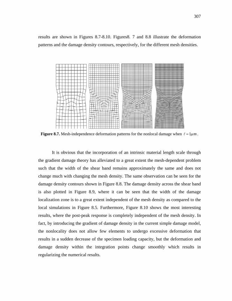
307
results are shown in Figures 8.7-8.10. Figures8. 7 and 8.8 illustrate the deformation
patterns and the damage density contours, respectively, for the different mesh densities.
Figure 8.7. Mesh-independence deformation patterns for the nonlocal damage when 1 m .
It is obvious that the incorporation of an intrinsic material length scale through
the gradient damage theory has alleviated to a great extent the mesh-dependent problem
such that the width of the shear band remains approximately the same and does not
change much with changing the mesh density. The same observation can be seen for the
damage density contours shown in Figure 8.8. The damage density across the shear band
is also plotted in Figure 8.9, where it can be seen that the width of the damage
localization zone is to a great extent independent of the mesh density as compared to the
local simulations in Figure 8.5. Furthermore, Figure 8.10 shows the most interesting
results, where the post-peak response is completely independent of the mesh density. In
fact, by introducing the gradient of damage density in the current simple damage model,
the nonlocality does not allow few elements to undergo excessive deformation that
results in a sudden decrease of the specimen loading capacity, but the deformation and
damage density within the integration points change smoothly which results in
regularizing the numerical results.

308
Figure 8.8. Mesh-independent results of the damage density contour on deformed configuration using the nonlocal damage model when 1 m . Damage accumulation and width of shear band
are mesh insensitive.
1152 elements
5000 elements
200 elements
512 elements

309
Figure 8.9. Mesh-independent results of damage density distribution across the shear band, along the path ‘a-a’, when 1 m .
Figure 8.10. Mesh-independent results of the predicted load-displacement diagrams when 1 m .
0.1
0.2
0.3
0.4
0.5
0.6
0.7
0.8
0.9
1
0.5 0.55 0.6 0.65 0.7 0.75 0.8 0.85 0.9
Dam
age
dens
ity
acro
ss t
he s
hear
ban
d
Normalized distance
200 elements
512 elements
1152 elements
5000 elements
0
500
1000
1500
2000
2500
3000
3500
4000
4500
5000
0 0.1 0.2 0.3 0.4 0.5 0.6 0.7
Loa
d (1
0-4N
)
Displacement (µm)
200 elements
512 elements
1152 elements
5000 elements

310
8.5.2. Strip in Tension
In the previous section, damage localization and evolution of a shear band in a plane
strain plate under tension was studied, and the ability of the nonlocal damage algorithm
in successfully providing mesh-objective results is demonstrated. In this section, the
same material properties are considered; however, the geometry is changed and
enhanced with an imperfection in order to enforce the formation of a shear band in a
specific direction. This is a common benchmark problem that is used to assess the ability
of damage/plasticity theory in achieving mesh-objective results. The problem geometry,
loading, and boundary conditions are shown in Figure 8.11. The strip is constrained at
the bottom and a displacement of 1 m is applied at the upper edge of the strip. Similar
to the previous section, four different meshes of 200, 512, 1152, and 5000 elements are
considered. A four-node plane strain quadrilateral element with four integration points is
used in the following simulations. Due to the specimen’s geometric imperfection, the
shear band initiates at the bottom left corner and evolves with an inclination of 45o. In
this case, the nonlinearity in geometry is investigated in the formation of a shear band
and in the distribution of the damage density across the shear band.
Figure 8.11. The geometry of the strip in tension.
10 m
20 m
10 5. m

311
In Figure 8.12 the obtained deformation patterns for all meshes when setting
0 are plotted. It can be observed easily that the width of the shear band is determined
by the element size when utilizing the classical continuum damage mechanics.
Deformation is localized almost within one element width.
Figure 8.12. Mesh-dependence of deformation patterns for the strip with an imperfection under tension when 0 . Non-physical response; deformation localizes within one element.
Mesh-dependence is also obvious from the damage density contours plotted in Figure
8.13 and the damage density across the shear band presented in Figure 8.14, where the
width of the shear band is strongly dependent on the mesh density.

312
Figure 8.13. Mesh-dependent results of damage density contour on deformed configuration using the classical continuum damage model with .
It should be noted that damage density value could not be more than one; hence,
the localization phenomenon appears in the form of width of the shear band not the
maximum value for damage density.
0
1152 elements
5000 elements
200 elements
512 elements

313
Figure 8.14. Damage density across the shear band when 0 . Width of the localized zone depends on the mesh density.
Nonlocal damage gradient algorithm is employed to remedy the mesh sensitivity
problem. Material properties of the specimen are assumed to be the same in both
examples. Hence, the same length scale of 1 m is also considered here to keep the
field equations well-posed. Figures 8.15 and 8.16 illustrate respectively the deformation
patterns and damage density contours for different mesh densities. As it is obvious from
the figures, the nonlocal damage algorithm solves the mesh-dependency problem to a
great extent. Moreover, a damage density across the shear band is depicted in figure
8.17, which also confirms mesh-independent shear band width. In order to show the
effect of nonlocal damage on the post-peak response, the load-displacement diagrams for
all mesh densities for both local, 0 , and nonlocal, 1 m , cases are plotted in
Figure 8.18. It is very clear from this figure that the current nonlocal damage model with
the proposed computational algorithm predicts mesh-independent post-peak response
whereas the local damage model is mesh-dependent. Also, it is obvious from this figure
that a non-zero length scale delays damage and smooth it out during the deformation
process.
0
0.1
0.2
0.3
0.4
0.5
0.6
0.7
0.8
0.9
1
0 0.2 0.4 0.6 0.8 1
Dam
age
dens
ity
acro
ss t
he s
hear
ban
d
Normalized distance
200 elements
512 elements
1152 elements
5000 elements

314
Figure 8.15. Mesh-independent deformation patterns when 1 m .
Figure 8.16. Mesh-independent results of damage density contour on deformed configurations when 1 m .Width of the shear band is almost the same for all mesh densities.
1152 elements
50000 elements
200 elements
512 elements

315
Figure 8.17. Mesh-independent results of damage density across the shear band when 1 m .
Figure 8.18. Load-Displacement diagrams showing the results for 0 and 1 m .
0
0.1
0.2
0.3
0.4
0.5
0.6
0.7
0.8
0.9
1
0 0.2 0.4 0.6 0.8 1
Dam
age
dens
ity
acro
ss t
he s
hear
ban
d
Normalized distance
200 elements
512 elements
1152 elements
5000 elements
0
500
1000
1500
2000
2500
3000
3500
4000
4500
5000
0 0.1 0.2 0.3 0.4 0.5 0.6 0.7 0.8
Loa
d (1
0-4N
)
Displacement (µm)
200 elements, L=0
512 elements, L=0
1152 elements, L=0
5000 elements, L=0
200 elements, L=1
512 elements, L=1
1152 elements, L=1
5000 elements, L=1
0000
1111

316
8.6. Effect of Different Parameters on Damage Localization
8.6.1. Effect of Parameters and
In this section, the effect of material constants in the damage force equation Eq. (8.3)
and in Eq. (8.8), on the location and width of shear band is investigated. The
parameter defines the material sensitivity to confinement whereas the parameter
represents the rate of damage growth. These parameters are selected as 0 and
0 1. in the previous examples. To study the effect of these parameters on the
development of damage localization, the nonlocal damage case for 1 m is simulated
for the intermediate mesh density for the fixed plate in tension examples.
The parameter in Eq. (8.3) controls the material sensitivity due to confinement
and mean stress. In other words, describes the fact that specimen with higher
compressive mean stress can tolerate more load without going to a damaged state.
However, in this problem the applied stress is tensile, so it is expected that the regions
with higher tensile stresses become damaged faster. The simulation results presented in
Figure 8.19(a) confirms the pressure sensitive results.
One can explain that due to Poisson’s effect, regions that are closer to the bottom
edge boundary undergo higher tensile stresses which can be characterized by the
negative mean stress. Hence, these regions should go to the damage region earlier. As it
is obvious from Figure 8.19(a), increasing the value of causes the shear band to move
slightly toward the bottom edge and for large values of the damaged region is very
close to the bottom. Furthermore, the load displacement diagram for different values of
is also shown in Figure 8.19(b). This figure shows that increasing the parameter
induces a softening effect and causes the specimen to go to the softening region faster.
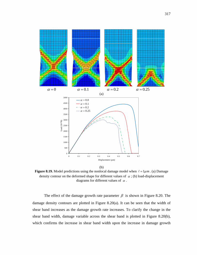
317
0 0 1. 0 2. 0 25.
(a)
(b) Figure 8.19. Model predictions using the nonlocal damage model when . (a) Damage
density contour on the deformed shape for different values of ; (b) load-displacement diagrams for different values of .
The effect of the damage growth rate parameter is shown in Figure 8.20. The
damage density contours are plotted in Figure 8.20(a). It can be seen that the width of
shear band increases as the damage growth rate increases. To clarify the change in the
shear band width, damage variable across the shear band is plotted in Figure 8.20(b),
which confirms the increase in shear band width upon the increase in damage growth
1 m
0
500
1000
1500
2000
2500
3000
3500
4000
4500
5000
0 0.1 0.2 0.3 0.4 0.5 0.6 0.7
Loa
d (1
0-4N
)
Displacement (µm)
Alpha=0.0
Alpha=0.1
Alpha=0.2
Alpha=0.25
0.0 0.1 0.2 0.25

318
rate. As it is expected, damage grows and distributes within the specimen faster for
larger damage growth rates. This effect can be seen clearly in the load-displacement
diagrams shown in Figure 8.20(c). Thus, higher damage growth rates make the specimen
to undergo the softening region faster and exhibits higher degree of softening.
0 1. 0 2. 0 3. 0 5.
(a)
(b) Figure 8.20. The effect of on (a) damage density contour on deformed shape, (b) damage
density across the shear band, (c) load-displacement diagram. Results are for .
1 m
0
0.1
0.2
0.3
0.4
0.5
0.6
0.7
0.8
0.9
1
0.1 0.2 0.3 0.4 0.5 0.6
Dam
age
dens
ity
Normalized distance
Beta=0.1
Beta=0.2
Beta=0.3
Beta=0.5
0.1
0.2
0.3
0.5

319
(c)
Figure 8.20. Continued.
From Figures 8.19 and 8.20, one can conclude that controls the location of shear
band and causes the shear band to form in regions with smaller confinement, whereas
controls the width of the shear band and rate of softening behavior.
8.6.2. Length Scale Effect
In this section, the effect of the length scale value on the width of shear band,
deformation pattern, and damage distribution across the shear band is presented. To this
aim, the fixed plate in tension with 1152 elements is selected. The specimens are loaded
until complete failure. Deformation patterns, damage density across the shear band, and
load-displacement diagrams are shown in Figures 8.21(a), 8.21(b), and 8.21(c),
respectively, for different values of . Figure 8.21(a) clearly shows that the width of the
shear band depends on the length scale value such that the larger the length scale value
the broader the shear band width as also clearly shown in Figure 8.21(b), which is a
known result (Pamin, 1994). This shows that the proposed computational algorithm yield
reasonable and physically known behavior. The damage distribution across the shear
band and the load-displacement diagrams for various length scales are shown in Figures
0
500
1000
1500
2000
2500
3000
3500
4000
4500
5000
0 0.1 0.2 0.3 0.4 0.5 0.6 0.7
Loa
d (1
0-4N
)
Displacement (µm)
Beta=0.1
Beta=0.2
Beta=0.3
Beta=0.5
0.1
0.2
0.3
0.5

320
8.21(b) and 8.21(c), respectively. Figure 8.21(b) shows that increasing the length scale
value causes the damage density to regularize more in the specimen. Figure 8.21(c)
shows that the length scale value is the parameter that delays damage initiation and
growth. Hence, materials with larger length scale values tolerate higher stresses
compared to the materials with smaller length scale values.
1 m 3 m 6 m 10 m
(a)
Figure 8.21. Effect of on (a) deformed pattern, (b) damage density across the shear band, (c)
load-displacement diagram. Nonlocal damage for .
1 3 6 and 10, , , m
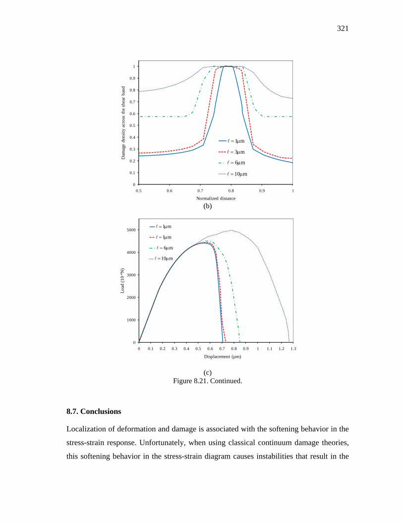
321
(b)
(c) Figure 8.21. Continued.
8.7. Conclusions
Localization of deformation and damage is associated with the softening behavior in the
stress-strain response. Unfortunately, when using classical continuum damage theories,
this softening behavior in the stress-strain diagram causes instabilities that result in the
0
0.1
0.2
0.3
0.4
0.5
0.6
0.7
0.8
0.9
1
0.5 0.6 0.7 0.8 0.9 1
Dam
age
dens
ity
acro
ss t
he s
hear
ban
d
Normalized distance
L=1
L=3
L=6
L=10
1 m
3 m
6 m
10 m
0
1000
2000
3000
4000
5000
0 0.1 0.2 0.3 0.4 0.5 0.6 0.7 0.8 0.9 1 1.1 1.2 1.3
Loa
d (1
0-4N
)
Displacement (µm)
L=1
L=3
L=6
L=10
1 m
1 m
10 m
6 m

322
loss of well-posedness of the governing partial differential equations and in turn lead to
mesh-dependent results and non-physical description of damage evolution and failure.
As shown by many authors, a very effective way to remedy this problem is through the
nonlocal gradient-enhanced damage theory. However, one of the most challenging issues
when dealing with this type of theories is their implementation in the finite element
codes. In this work, a simple and straightforward computational approach is presented
for numerically integrating the nonlocal constitutive equations with little effort required
to modify an existing finite element code. Hence, by using this approach, one can avoid
the common practice in introducing high-order continuous shape functions (e.g. C1 class
or penalty-enhanced C0 class functions) with additional degrees of freedom in a finite
element code to calculate the gradient terms, which is computationally difficult and
expensive. A simple algorithm for satisfying damage consistency condition is proposed
which can be implemented easily in a finite element code. Numerical algorithm
presented in this paper is implemented in the well-known finite element code Abaqus via
the user material subroutine UMAT. The effectiveness and robustness of the proposed
approach in alleviating the mesh-dependency problem when simulating damage
localization and the post-peak response are illustrated through two numerical examples.
The examples show that results of the shear band converge to a unique solution upon
mesh densification and clearly show that the proposed computational algorithm works
well in integrating the nonlocal damage theories. Moreover, a parametric study on the
effect of the material constants associated with the presented elastic-damage model is
conducted with special emphasis placed on their effect on the size of the localized
damage zone and the post-peak response. Finally, the proposed numerical algorithm can
be easily adapted by more complex constitutive models that incorporate the effect of
higher-order gradients.
The proposed general numerical technique along with the developed constitutive
model will be employed in the next chapter to investigate the best way for predicting the
performance simulation of asphalt pavements.

323
CHAPTER IX
FINITE ELEMENT AND CONSTITUTIVE MODELING
TECHNIQUES FOR PREDICTING RUTTING IN ASPHALT
PAVEMENTS
9.1. Introduction
This chapter focuses on a comprehensive evaluation of the effects of different finite
element (FE) modeling techniques and material constitutive models on predicting rutting
in asphalt pavements under repeated loading conditions. Different simplified two-
dimensional (2D) and more realistic three-dimensional (3D) loading techniques are
simulated and compared for predicting asphalt rutting. This study also evaluates and
compares the rutting performance predictions using different material constitutive
behaviors such as viscoelastic-viscoplastic, elasto-viscoplastic, and coupled viscoelastic,
viscoplastic, and viscodamage behaviors.
Rutting is one of the most serious distresses in asphalt pavements affecting the
pavement performance and service life. Therefore, the accurate simulation of rutting in
asphalt pavements is essential for improving their performance and management. The
main mechanism of rutting is the accumulation of permanent deformation that increases
progressively with increasing number of loading cycles. However, the complex nature of
the applied loading conditions, very large number of loading cycles (millions of loading
cycles), and complex constitutive behavior of asphaltic materials make the accurate
prediction of rutting a very difficult and challenging task. Even with the current state-of-
the-art in computational power, conducting 3D finite element (FE) rutting performance
simulations for pavements subjected to millions of wheel loading cycles and considering
realistic wheel tracking and environmental loading conditions is almost impossible.
Therefore, an evaluation of a simplified numerical model with efficient and realistic
loading conditions and material constitutive models that can simulate the pavement
rutting performance for a very large number of loading cycles is desirable. In order to
accurately simulate the pavement response, the computer simulations should have the

324
capability to capture the response by considering structural loading, boundary
conditions, and material constitutive behavior. Therefore, realistic loading and boundary
conditions should be imposed, and an accurate material constitutive model should be
utilized. The material model should be able to describe the inelastic-damage behavior of
asphalt under different stress levels, loading rates, and temperatures.
At the material level, experimental measurements show that the deformation
response of asphaltic materials is time-, rate-, and temperature-dependent such that the
accurate constitutive model should at least consider the couplings between the
temperature, viscoelasticity, viscoplasticity, and viscodamage models. Therefore, the
constitutive model presented in Chapter II is used here to investigate the effect of each
component of the constitutive model on rutting performance simulation of asphalt
pavements.
In terms of the FE modeling of asphaltic pavements under simplified loading
conditions, several FE studies have been conducted in order to predict the rutting
performance. Lu and Wright (1998) constructed a two-dimensional (2D) plane strain FE
model to represent a three layers pavement structure and employed the Perzyna’s
viscoplastic model to predict the permanent deformation under large number of loading
cycles assuming a pulse loading. Pulse loading is commonly used to represent a wheel
moving load. However, the implicit assumption in conducting 2D plane strain FE
simulations is that the loading condition is represented as an infinite load strip in the
traffic direction (see Table 9.1). Similarly, Hunter et al. (2007) have also conducted 2D
plan strain FE simulations of the Wheel Tracking Test in order to predict rutting
performance assuming a pulse loading. However, Hunter et al. (2007) have used a power
law viscoplasticity constitutive model and neglected viscoelasticity and damage
evolution. Their simulations show that the shape of rutting is significantly different than
that obtained experimentally. Kettil et al. (2007) have conducted 2D axisymmetric FE
simulations and compared two different loading assumptions; pulse loading and
equivalent loading (see Table 9.1).

325
Table 9.1. Summary of simulated loading assumptions.
Mode Loading approach Loading Area Schematic representation of loading modes
1 (2D) Pulse loading (plane strain)
One wheel
2 (2D) Equivalent loading
(plane strain) One wheel
3 (2D) Pulse loading
(axisymmetric) One wheel
4 (2D) Equivalent loading
(axisymmetric) One wheel
5 (3D) Pulse loading One wheel
6 (3D) Equivalent loading One wheel
7 (3D) Pulse loading Whole wheel path
8 (3D) Equivalent loading Whole wheel path
9 (3D) Pulse loading Circular loading
area
10 (3D) Equivalent loading Circular loading
area
11 (3D) Moving loading One wheel
The equivalent loading assumption, which is another commonly adapted loading
assumption to represent a wheel moving load, applies the wheel loading over the
Moving Direction

326
respective accumulative loading time neglecting the unloading time periods. Results
from this study showed that the equivalent loading assumption gives comparable rutting
performance predictions from the pulse loading assumption such that by assuming an
equivalent loading one can save significant amount of computational time. However, this
conclusion is based on assuming an elasto-viscoplastic material behavior neglecting the
viscoelastic and damage behavior of asphaltic materials. Cho et al. (1996) compared the
rutting predictions from 2D plane strain, 2D axisymmetric, and 3D FE simulations
assuming a linear elastic behavior of the asphalt material. Huang et al. (2001) conducted
2D and 3D axisymmetric simulations of asphalt pavement sections using an elasto-
viscoplastic model. Results of this research showed that the 3D FE analysis gives more
accurate predictions as compared to field measurements. Huang (1995) proposed a step
loading function to simulate a large number of loading cycles of a moving load in 3D FE
simulations. This loading function accumulates each wheel pass time to produce a total
cumulative loading time and then applies a single load step to a set of elements in the
middle of the whole wheel path. Hua (2000) improved the cumulative loading time
approach by Huang (1995). The improved approach also accumulates each single
loading time, and then applies a single step loading on the whole wheel path to represent
the moving wheel loading in 3D simulations. However, in both of these works [i.e.
Huang (1995) and Hua (2000)] an elasto-viscoplastic model is used for validating the
proposed loading models. Huang (2001), Hua and White (2002), and Park et al. (2005)
used an elasto-viscoplastic model along with the cumulative loading time approach to
represent a large number of loading cycles. Saleeb et al. (2005) used a visco-elasto-
plastic model to conduct a 3D FE simulation with a moving loading model by applying
the loading on one set of elements and then moving forward to the next set of elements.
However, most of the aforementioned FE simulations have focused on the effect of
loading modes. To the authors’ best knowledge, no study yet has used a comprehensive
constitutive model incorporating nonlinear viscoelasticity, viscoplasticity, and
viscodamage for simulating rutting performance of asphalt pavements.

327
The main objective of this work is to study the effect of different simplified
wheel loading assumptions on 2D and 3D FE rutting simulations of asphalt layers using
different constitutive behaviors; namely, elasto-viscoplastic, viscoelastic-viscoplastic,
and coupled viscoelastic-viscoplastic-viscodamage constitutive behaviors. Different
simplified two-dimensional (2D) and more realistic three-dimensional (3D) finite
element (FE) loading techniques that represent the commonly conducted Wheel
Tracking Test are simulated and compared to predict asphalt rutting performance.
The simulations show that the assumption of the equivalency between a pulse
loading and an equivalent loading, which are commonly used as simplified loading
assumptions for predicting rutting, is reasonable for viscoelastic-viscoplastic and elasto-
viscoplastic constitutive behaviors. However, these loading assumptions and material
constitutive models overestimate rutting as damage grows. Results show that the 2D
plane strain FE simulations significantly overestimate rutting as compared to the rutting
performance predictions from more realistic 3D FE simulations (Abu Al-Rub et al.,
2011).
9.2. Material Constitutive Model
The coupled thermo-viscoelastic-viscoplastic-viscodamage constitutive model presented
in Chapter II is used to conduct this study. This constitutive model is not presented in
this chapter in order to avoid the repetition. Please refer to Chapter II for a
comprehensive and detailed description of the constitutive model.
9.3. Description of the Finite Element Simulations
This section presents the description of 2D and 3D FE rutting simulations of a test
asphalt slab in a Wheel Tracking Test, and the description of the employed wheel
loading assumptions for simplifying the FE simulations.

328
9.3.1. Geometry of the Finite Element Model
This study simulates the Wheel Tracking Test as an example to investigate the effect of
various commonly adapted loading assumptions on rutting predictions. Based on this
analysis, one can draw conclusions about the suitability and computational cost of each
loading assumption in predicting the rutting in asphaltic layers. The geometry of the
Wheel Tracking Test is illustrated in Figure 9.1.
Figure 9.1. The geometry of the simulated Wheel Tracking Test. (a) X-Y plane; (b) Y-Z plane.
The wheel tracking test consists of an asphalt slab of dimensions of 305280
100 mm3 in length, width, and depth, respectively. A wheel load is applied at the middle
of the slab along the width and moved bake and forth along the length of the slab. The
Symmetry
Position A
x
y
280 mm
305 mm
50 mm
230 mm
20 mm
280 mm
100 mm
Wheel Path
One loading area (Position B)
(a) (b)
z
y Position C

329
wheel moves with a speed of 40 passes per minute over a wheel path of 230mm length,
which is equivalent to a 0.55 km/hr speed. The wheel loading area is assumed as a
rectangular shape with dimensions of 2050 mm2 in width and length, respectively. The
employed asphalt layer, dimensions of the loading area, and the wheel speed are from
the Wheel Tracking Test conducted by Hunter et al. (2007). The loading is applied as a
step load within each loading cycle. Because of the symmetric nature of the wheel
loading condition and the slab’s geometry, the finite element model can be reduced to a
half of the slab by constraining the horizontal direction on the vertical edge of the model
to represent the middle of the slab.
The 3D and 2D finite element meshes showing the applied wheel loading are
shown in Figures 9.2(a) and 9.2(b), respectively.
(a) (b) Figure 9.2. The FE mesh in (a) the 3D simulations and (b) the 2D simulations.
The boundary conditions in both 2D and 3D FE models are imposed such that the
horizontal direction on the opposite side of the symmetric boundary is fixed; while the
bottom of the slab is fixed in the vertical direction. The used element types in the 2D FE
simulations in Abaqus are plane strain four-node element with reduced integration
(CPE4R) for plane strain analysis, and axisymmetric four-node element with reduced

330
integration (CAX4R) for axisymmetric analysis; whereas, 3D eight-node element with
reduced integration (C3D8R) is used for conducting 3D FE simulations. Moreover, a
maximum element aspect ratio of 2 is used for the 2D and 3D elements, respectively.
According to the performed convergence studies for the 2D simulations, 2.52.5 mm2
elements are used under and close to the loads, whereas, the maximum element size of 5
5 mm2 is used for the area far from the loading path. For the 3D simulations, 2.52.5
2.5 mm3 elements are used under the load and close to loading path, whereas, the
maximum element size of 555 mm3 is used for the regions that are far from the
loading path. From a convergence study that is not reported here, the constructed 2D and
3D meshes were sufficient to get converged results that are independent of the mesh
density. The loading level is 770 kPa and is applied on the top of the asphalt layer with
different loading scenarios as described in the next section. For simplicity, the shape of
the applied load is assumed rectangular. Moreover, frictional and tangential loadings
from the contact of the wheel with the asphalt top surface are neglected in this study.
9.3.2. Applied Wheel Loading Assumptions
The loading modes (or loading assumptions) can be categorized into two main types (see
Table 9.1): (1) loading duration such as pulse loading, equivalent loading, and moving
loading; and (2) loading area such as applying the loading on one wheel area, on the
whole wheel path, and on a circular loading area that represents the axisymmetric
analysis. Considering the combination of those loading categories, four loading modes
can be considered in the 2D simulations; whereas seven loading modes can be
considered in the 3D simulations (see Table 9.1). Those loading modes are applied to the
2D and 3D FE models and then the results are compared in terms of the rutting
performance in order to find an efficient loading mode, but simple enough, for the
prediction of rutting under very large number of repeated loading cycles. Therefore, the
objective from simulating these loading scenarios is to identify a loading assumption that
allows one to predict effectively and with minimum computational cost the rutting
performance of asphaltic layers over a large number of repeated loading cycles without
the need of complicated and computationally expensive rutting performance simulations.

331
9.3.2.1. Wheel loading assumptions in 2D simulations
In the 2D FE simulations, two cases are considered for the area on which the loading is
applied: (1) the loading is applied on an infinite stripe bar along the length of the
pavement; (2) the loading is applied on a circular area at the middle of the pavement.
The first case is simulated using 2D plane strain FE models, whereas the second case is
simulated using 2D axisymmetric FE models. Moreover, two loading durations are
assumed for each of the cases. The first loading duration is a pulse loading in which the
wheel load is applied with a loading time period of 0.109 sec and then the load is
removed for 0.109 sec as shown in Table 9.1 and Figure 9.3.
Figure 9.3. The sketch of equivalent and pulse loading modes. Equivalent loading is obtained by substituting pulse loading by a one step equivalent loading whose duration is equal to the
summation of loading times in pulse loading.
The simulated total loading-unloading cycles in this case are 1000 cycles. The
loading scheme is shown in Figure 9.3(a). The second loading duration is the equivalent
…………… N cycles
Unloading time
Time N* LT
Loading time (LT)
(b) Equivalent loading mode
(a) Pulse loading mode
Stress

332
loading mode (Mode 2) as shown in Table 9.1 and Figure 9.3(b). This loading
assumption represents the equivalent loading time by accumulating the loading time
from all loading cycles and then applying the wheel loading at once in one loading cycle
for the period of accumulated time such that the unloading or resting time is neglected.
The advantage of this loading model is that only one step loading is applied instead of
applying large number of loading steps, and thus reducing greatly the computational
cost. Hence, four loading assumptions are considered in the 2D simulations (see Table
9.1).
9.3.2.2. Wheel loading assumptions in 3D simulations
In the 3D FE simulations as compared to the 2D simulations, one can specify the loading
location and apply more realistic loading conditions. In the 3D simulations, seven wheel
loading scenarios can be simulated. The fifth loading assumption (Mode 5) as shown in
Table 9.1 assumes a pulse loading (as described in Modes 1 and 3) where the load is
applied at the center of the asphalt layer (position B in Figure 9.1) with one wheel
loading area. As shown in Figure 9.3 the loading duration is 0.109 sec and also 0.109 sec
for the unloading within each cycle. A 1000 loading-unloading cycles are applied in this
case. The sixth loading scenario (Mode 6) assumes an equivalent loading time (as
described in Modes 2 and 4) where one wheel loading area is applied at position B in
Figure 9.1 Loading modes 7 and 8 assume a pulse loading (loading time of 0.109 sec and
unloading time of 0.109 sec) and an equivalent time loading, respectively. Both modes 7
and 8 assume the loading over the whole wheel path (shown in Figure 9.1). Moreover, a
circular loading area is assumed for modes 9 and 10. A pulse loading and an equivalent
time loading are assumed for loading modes 9 and 10, respectively. Finally, the last
loading mode is the moving loading (Mode 11) where the wheel movement is simulated
by applying the wheel loading on one set of elements (one loading area) at the beginning
of the wheel path (position A in Figure 9.1). This load remains on the shaded area shown
in Figure 9.4(a) for 0.109 sec ( 2 1t t ) and then moving it forward to the next set of
elements shown in Figure 9.4(b). The load remains on the same set of elements shown in
Figure 9.4(b) for the same loading duration of 0.109 sec ( 3 2t t ) and then moves to

333
another set of elements shown in Figure 9.4(c) until it reaches to the end of the wheel
path (position C in Figure 9.1). This loading mode, which is illustrated in Figure 9.4, is
the most realistic one as compared to the aforementioned loading modes. This approach
of simulating the moving load is followed in the current study due to its simplicity and
the significant reduction in the computational cost as compared to explicitly simulating a
real tire with considering dynamic effects.
(a)
(b)
(c)
Figure 9.4. A schematic representation of the simplified wheel moving loading scenario. The shaded area is the region at which the wheel load is applied over a set of elements and then
moved in the traffic direction to a new set of elements.
It should be noted that one would expect different rutting results using plane
strain simulations (loading modes 1 and 2) or using their 3D counterparts (loading
modes 7 and 8) comparing to the realistic loading conditions. However, the qualitative
comparison of the changes in the results using these simplifications is of great
importance in deciding on when to use these simplifications depending on the problem
under study.
9.4. Material Parameters
The asphalt mix used in the Wheel Tracking test is the same as the asphalt mix used in
Chapter II. Therefore, the viscoelastic, viscoplastic, and viscodamage model parameters
3t t
2t t
1t t
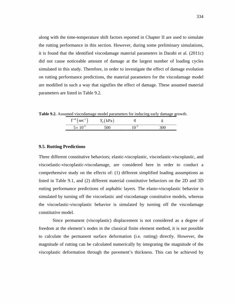
334
along with the time-temperature shift factors reported in Chapter II are used to simulate
the rutting performance in this section. However, during some preliminary simulations,
it is found that the identified viscodamage material parameters in Darabi et al. (2011c)
did not cause noticeable amount of damage at the largest number of loading cycles
simulated in this study. Therefore, in order to investigate the effect of damage evolution
on rutting performance predictions, the material parameters for the viscodamage model
are modified in such a way that signifies the effect of damage. These assumed material
parameters are listed in Table 9.2.
Table 9.2. Assumed viscodamage model parameters for inducing early damage growth.
-1secvd 0 kPaY q k
5 10-5 500 10-5 300
9.5. Rutting Predictions
Three different constitutive behaviors; elastic-viscoplastic, viscoelastic-viscoplastic, and
viscoelastic-viscoplastic-viscodamage, are considered here in order to conduct a
comprehensive study on the effects of: (1) different simplified loading assumptions as
listed in Table 9.1, and (2) different material constitutive behaviors on the 2D and 3D
rutting performance predictions of asphaltic layers. The elasto-viscoplastic behavior is
simulated by turning off the viscoelastic and viscodamage constitutive models, whereas
the viscoelastic-viscoplastic behavior is simulated by turning off the viscodamage
constitutive model.
Since permanent (viscoplastic) displacement is not considered as a degree of
freedom at the element’s nodes in the classical finite element method, it is not possible
to calculate the permanent surface deformation (i.e. rutting) directly. However, the
magnitude of rutting can be calculated numerically by integrating the magnitude of the
viscoplastic deformation through the pavement’s thickness. This can be achieved by

335
dividing the thickness of the asphalt layer into a number of sub-layers, such that the
rutting depth can be calculated as follows:
1
kvp i i
ruttingi
u h
(9.1)
where ruttingu is the permanent displacement (rutting), vp i is the vertical viscoplastic
strain at ith layer through the depth of the asphalt layer, and ih is the ith layer thickness.
In the following, the rutting is only calculated at the center of the slab (position B in
Figure 9.1) for the purpose of conducting the numerical comparisons.
9.5.1. 2D Simulation Results
As it was mentioned, four loading scenarios can be assumed for performing the 2D FE
simulations for predicting rutting as shown in Table 9.1 (i.e. Mode 1: plane strain-pulse
loading; Mode 2: plane strain-equivalent loading; Mode 3: axisymmetric-pulse loading;
and Mode 4: axisymmetric-equivalent loading). In the 2D plane strain simulations, it is
assumed that the loading is applied as an infinite strip along the length of the asphalt
layer. The corresponding 3D loading modes for the 2D loading modes 1 and 2 are
loading modes 7 and 8, respectively. Furthermore, for the 2D axisymmetric simulations,
the loading is assumed to be applied on a circular area. Hence, the corresponding 3D
loading modes for the 2D loading modes 3 and 4 are loading modes 9 and 10. Figures
9.5 and 9.6 show the rutting versus loading cycles assuming a viscoelastic-viscoplastic
constitutive behavior at temperatures 20 oC and 40 oC, respectively. Figures 9.5 and 9.6
show that the rutting values obtained from the pulse and equivalent loading cases are
comparable. However, the difference depends on the employed constitutive model and
decreases as the temperature increases. The 2D simulation results assuming an elasto-
viscoplastic material behavior are shown in Figure 9.7. This figure shows that an elasto-
viscoplastic constitutive behavior leads to prediction of the same rutting values for pulse
and equivalent loading cases when the only difference is the loading duration (i.e. pulse
loading versus equivalent loading).

336
Figure 9.5. The rutting results for 2D plane strain and axisymmetric and their corresponding 3D FE simulations at temperature 20 oC assuming a nonlinear viscoelastic and viscoplastic material
constitutive behavior.
Figure 9.6. The rutting results for 2D plane strain and axisymmetric and their corresponding 3D FE simulations at temperature 40 oC assuming a nonlinear viscoelastic and viscoplastic material
constitutive behavior.
0
0.02
0.04
0.06
0.08
0.1
0.12
0 200 400 600 800 1000
Rut
ting
(mm
)
Cycles (N)
Loading Mode 1 Loading Mode 2
Loading Mode 3 Loading Mode 4
Loading Mode 7 Loading Mode 8
Loading Mode 9 Loading Mode 10
0
0.02
0.04
0.06
0.08
0.1
0.12
0.14
0.16
0 200 400 600 800 1000
Rut
ting
(mm
)
Cycles (N)
Loading Mode 1 Loading Mode 2
Loading Mode 3 Loading Mode 4
Loading Mode 7 Loading Mode 8
Loading Mode 9 Loading Mode 10

337
Figure 9.7. The rutting results for 2D plane strain and axisymmetric and their corresponding 3D
FE simulations at temperature 20 oC assuming an elasto-viscoplastic material constitutive behavior.
The 2D simulation results for loading modes 1-4 when damage is activated are
shown in Figure 9.8. Figure 9.8 shows that when damage is activated the simulation
results for loading modes 1 and 2 could be very different. This is attributed to the
viscous behavior of the damage law. In other words, changing the loading duration has a
significant effect on the value of damage density since the damage law is time-
dependent. These observations clearly show that the differences in rutting values using
different simplified loading assumptions are also model-dependent. For example, these
differences are magnified when the damage component of the model is added to the
viscoelastic-viscoplastic constitutive model. Also, one may expect greater differences if
other material mechanisms such as the viscoplastic softening (i.e. decrease levels of
viscoplastic hardening during each loading cycle due to rearrangements in the material’s
microstructure) which is related to the loading history is considered. In other words, any
material mechanism which is related to the loading history could magnify the differences
in calculated rutting values using the simplified loading assumptions and realistic
loading scenarios since the simplified loading assumptions do not capture the real
loading history. Therefore, it should be emphasized that the rutting predictions from a
0
0.02
0.04
0.06
0.08
0.1
0.12
0 200 400 600 800 1000
Rut
ting
(mm
)
Cycles (N)
Loading Mode 1 Loading Mode 2
Loading Mode 3 Loading Mode 4
Loading Mode 7 Loading Mode 8
Loading Mode 9 Loading Mode 10

338
specific simplified loading assumption completely depends on the employed constitutive
model and one cannot generalize the conclusions from a specific loading assumption
independent of the employed constitutive model.
Figure 9.8. The rutting results for 2D plane strain and axisymmetric and their corresponding 3D
FE simulations at temperature 20 oC using the coupled viscoelastic-viscoplastic-viscodamage material constitutive model.
The same trend is also obtained from the simulation results of loading modes 3
and 4. The results of loading modes 7 and 8, which are the 3D counterparts of loading
modes 1 and 2, respectively, are also presented in Figures 9.5-9.8. These figures show
that the results of loading modes 1 and 7, and the results of loading modes 2 and 8 are
very similar. Details of the 3D simulations are presented in the following section.
As an example, the viscoplastic strain and damage contours at different loading
cycles for loading mode 1 is plotted in Figures 9.9 and 9.10, respectively, for the
viscoelastic-viscoplastic-viscodamage model. Figure 9.9 shows that the maximum
viscoplastic strain occurs at the half top portion of the pavement. Figure 9.10 shows that
the maximum damage occurs at the top of the middle part of the asphalt layer which is
exactly the region where the maximum viscoplastic strain occurs. However, as it is clear
0
0.02
0.04
0.06
0.08
0.1
0.12
0.14
0.16
0 200 400 600 800 1000
Rut
ting
(mm
)
Cycles (N)
Loading Mode 1 Loading Mode 2
Loading Mode 3 Loading Mode 4
Loading Mode 7 Loading Mode 8
Loading Mode 9 Loading Mode 10

339
from Figure 9.10, damage does not distribute toward bottom part of the asphalt layer
instead it localizes at the top of the middle part of the asphalt layer that eventually causes
macro-cracks at that region. These macro-cracks then propagate toward the surface of
the asphalt layer.
It is noteworthy that due to the large computational cost the rutting simulations of
this study are conducted up to 1000 loading cycles which is much lower than the actual
number of loading cycles in the wheel tracking tests. Hence, it is not a surprise that the
predicted values for the surface rutting is lower than the actual rutting values in the
wheel tracking tests which are conducted for huge number of cycles.
Figure 9.9. Viscoplastic strain distribution contours at different loading cycles for the 2D FE analysis when using the coupled viscoelastic-viscoplastic-viscodamage constitutive model at
20oT C when simulating the pulse loading (loading mode 1).
N=600 cycles
N=400 cycles
N=100 cycles
N=200 cycles

340
Figure 9.10. Damage distribution contours at different loading cycles for the 2D FE analysis
when using the coupled viscoelastic-viscoplastic-viscodamage constitutive model at 20oT C when simulating the pulse loading (loading mode 1).
However, the main purpose of this study is qualitative comparisons of rutting
values obtained from different simplified assumptions on the constitutive model and on
the imposed loading scenario with the most realistic constitutive model and loading
scenario, which are viscoelastic, viscoplastic, viscodamage model and the moving load
scenario, respectively, are used as a reference for qualifying the rutting predictions.
Although this study provides a qualitative comparison between different assumptions for
low number of loading cycles, the trend for larger number of loading cycles is expected
N=400 cycles
N=600 cycles
N=100 cycles
N=200 cycles

341
to be similar. The authors are currently working on developing an extrapolation
technique that could be used to extrapolate the 3D simulation results obtained from low
number of loading cycles to the simulation results for a large number of loading cycles.
9.5.2. 3D Simulation Results
Seven simplified loading scenarios are simulated for the 3D case. Figures 9.11 and 9.12
show the rutting predictions versus the number of loading cycles at temperatures 20 oC
and 40 oC, respectively.
Figure 9.11. The rutting simulation results from 3D FE analysis at temperature 20 oC assuming a
nonlinear viscoelastic and viscoplastic material constitutive behavior.
These results are obtained assuming that asphalt material behavior is
viscoelastic-viscoplastic with no damage. Since the rutting predictions from the moving
load (Mode 11) are the closest to the real loading in a Wheel Tracking Test, these figures
show that applying the loading over the whole wheel path (Modes 7 and 8) results in a
significant error in predicting rutting as compared to the moving load (mode 11). Figures
9.11 and 9.12 show that the axisymmetric assumption also overestimates the rutting
value as compared to the most realistic loading mode (mode 11). However, these figures
0
0.02
0.04
0.06
0.08
0.1
0.12
0.14
0 200 400 600 800 1000
Rut
ting
(mm
)
Cycles (N)
Loading Mode 5
Loading Mode 6
Loading Mode 7
Loading Mode 8
Loading Mode 9
Loading Mode 10
Loading Mode 11

342
show that cases when the wheel loading is only applied on one wheel loading area
(Modes 5 and 6) reasonably predict the simulation results of loading mode 11. Due to
the very large computational cost in conducting the moving load simulations, the results
are obtained up to about 400 and 500 cycles at temperatures 20 oC and 40 oC,
respectively. In terms of the effect of the pulse and equivalent loading conditions (Mode
5 versus 6; Mode 7 versus 8; Mode 9 versus 10), one can notice from Figures 9.11 and
9.12 that the rutting predictions are close when applying Mode 5 versus Mode 6, Mode 7
versus Mode 8, and Mode 9 versus Mode 10.
Figure 9.12. The rutting simulation results from 3D FE analysis at temperature 40 oC assuming a
nonlinear viscoelastic and viscoplastic material constitutive behavior.
Figure 9.13 shows the relationship between the rutting predictions and the
number of loading cycles when assuming an elasto-viscoplastic material constitutive
behavior with no viscoelasticity and no damage. Figure 9.13 shows that using pulse and
equivalent loading modes give comparable predictions when assuming that the loading
area is the same. This observation is compatible with the 2D simulation results shown in
Figure 9.7. As inferred from the results in Figures 9.11 and 9.12, the rutting predictions
from the loading Modes 5 and 6 are close to that from the moving loading mode (Mode
0
0.02
0.04
0.06
0.08
0.1
0.12
0.14
0.16
0 200 400 600 800 1000
Rut
ting
(mm
)
Cycles (N)
Loading Mode 5 Loading Mode 6
Loading Mode 7 Loading Mode 8
Loading Mode 9 Loading Mode 10
Loading Mode 11

343
11). However, when assuming loading Modes 7, 8, 9, and 10 the rutting is over predicted
significantly.
Figure 9.13. The rutting simulation results from 3D FE analysis at temperature 20 oC assuming
an elasto-viscoplastic material constitutive behavior.
In order to study the effect of damage on rutting using different loading modes in the 3D
simulations, the viscoelastic-viscoplastic-viscodamage constitutive model is now used.
Figure 9.14 shows the corresponding results at temperature 20 oC.
It is clear from Figure 9.14 that the rutting predictions are different for each
loading mode and the difference increases as damage grows. Figure 9.14 also shows that
when damage is activated, results from loading mode 11 (i.e. moving load) significantly
deviates from the results of loading modes 5 and 6 as compared to that in Figures 9.11-
9.13. This is attributed to the viscous behavior of the damage law. In other words,
changing the loading duration has a significant effect on the value of damage density
since the damage law is time-dependent. Moreover, it is found that the identified
viscodamage material parameters in Darabi et al. (2011c) did not cause noticeable
amount of damage at the largest number of loading cycles simulated in this study.
0
0.02
0.04
0.06
0.08
0.1
0.12
0.14
0 200 400 600 800 1000
Rut
ting
(mm
)
Cycles (N)
Loading Mode 5
Loading Mode 6
Loading Mode 7
Loading Mode 8
Loading Mode 9
Loading Mode 10
Loading Mode 11

344
Figure 9.14. The rutting simulation from 3D FE analysis at temperature 20 oC using the coupled
viscoelastic-viscoplastic-viscodamage material constitutive model.
Therefore, in order to investigate the effect of damage evolution on rutting
performance predictions, the material parameters for the viscodamage model are
modified in such a way that signifies the effect of damage. These assumed material
parameters also contribute in magnifying the differences in the predicted rutting values
using loading modes 5 and 6. The total loading duration for loading mode 11 is larger
than the loading duration for other loading modes and, therefore, the rate of rutting
accumulation and damage density from loading mode 11 are greater than those from
other loading modes (i.e. modes 5-10). Figure 9.15 shows the evolution of the maximum
damage density (occurring at the center of the loading and 30 mm from the top surface)
for different loading modes, where the damage density evolves differently depending on
the loading model and loading duration, but is much more important for loading mode
11 which causes the noticeable deviation from loading modes 5-10. Hence, one can
conclude that it is not accurate to substitute the pulse loading with equivalent loading in
the presence of significant damage. Also, substitution of loading mode 11 (moving load)
with loading modes 5 and 6 may cause significant error when damage is activated.
Figure 9.16 compares the rutting predictions for loading mode 11 when different
0
0.02
0.04
0.06
0.08
0.1
0.12
0.14
0 200 400 600 800 1000
Rut
ting
(mm
)
Cycles (N)
Loading Mode 5 Loading Mode 6
Loading Mode 7 Loading Mode 8
Loading Mode 9 Loading Mode 10
Loading Mode 11

345
constitutive models are used. These results show that the effect of using different loading
assumptions totally depends on the material constitutive model adapted for conducting
the rutting simulations.
Figure 9.15. The evolution of the damage density from 3D FE analysis at temperature 20 oC
using the coupled viscoelastic-viscoplastic-viscodamage material constitutive model.
Figure 9.16. Comparing the rutting predictions from the 3D FE simulations using different
constitutive models at temperature 20 oC for loading mode 11.
0
0.05
0.1
0.15
0.2
0.25
0.3
0.35
0.4
0 200 400 600 800 1000
Dam
age
dens
ity
Cycles (N)
Loading Mode 5
Loading Mode 6
Loading Mode 7
Loading Mode 8
Loading Mode 9
Loading Mode 10
Loading Mode 11
0
0.01
0.02
0.03
0.04
0.05
0.06
0 100 200 300 400 500 600
Rut
ting
(mm
)
Cycles (N)
Elasto-Viscoplastic Model
Viscoelastic-Viscoplastic Model
Viscoelastic-Viscoplastic-Viscodamage Model

346
As an example, the evolution of viscoplastic strain distribution at different
loading cycles for the loading mode 7 is plotted in Figure 9.17. Figure 9.17 shows that
the maximum viscoplastic strain occurs at the top of the middle part of the asphalt layer
which is consistent with the 2D predictions in Figure 9.9 and previous studies.
Moreover, it also shows that as the number of loading cycles increases, the compressive
viscoplastic strain extends toward both top and bottom of the pavement which
contributes to more permanent deformation.
Figure 9.17. Viscoplastic strain distribution contours at different loading cycles for the 3D FE analysis when using the coupled viscoelastic-viscoplastic-viscodamage constitutive model at
20oT C when simulating the pulse loading (loading mode 5).
N=400 cycles
N=600 cycles
N=100 cycles
N=200 cycles

347
Also, damage distribution contours are plotted for the same problem in Figure
9.18 which shows that the maximum damage occurs at the top of the middle part of
asphalt layer which is exactly the region where the maximum viscoplastic strain occurs.
The results in Figure 9.17 and 9.18 are consistent with the 2D viscoplasticity and
damage contours (Figures 9.9 and 9.10).
Figure 9.18. Damage distribution contours at different loading cycles for the 3D FE analysis
when using the coupled viscoelastic-viscoplastic-viscodamage constitutive model at 20oC when simulating the pulse loading (loading mode 5).
N=400 cycles
N=600 cycles
N=100 cycles
N=200 cycles

348
From the 3D FE predictions of rutting (Figures 9.11-9.14), one can conclude that
the simplified loading and constitutive assumptions can significantly affect the rutting
predictions. The difference between the rutting values using the moving load (Mode 11),
which is the most realistic one, and using the equivalent loading mode (Mode 8), which
is the most common loading assumption in the literature, exceeds 100% in some cases.
Moreover, assuming the equivalency between the pulse loading modes (Modes 7 and 9)
and the equivalent loading modes (Modes 8 and 10) totally depend on the assumed
constitutive model. This assumption yields almost similar results for an elasto-
viscoplastic constitutive model. It could also be reasonable for a viscoelastic-viscoplastic
constitutive mode; however, special care should be taken in the presence of damage
since the results of these two loading cases could be totally different; depending on the
damage level.
The conducted simulations show that rutting predictions in asphaltic pavements
using the simplified assumptions such as the 2D analysis instead of the 3D analysis and
using the equivalent loading assumption instead of the pulse loading assumption will
significantly overestimate rutting, but, on the other hand, significantly reduce the
computational cost. However, due to the very large computational cost needed to predict
the rutting using 3D FE simulations with a complex coupled viscoelastic, viscoplastic,
and viscodamage constitutive mode, it is imperative that an extrapolation technique to
very large number of cycles is developed based on 3D FE simulations.
9.6. Extrapolation of the Rutting in 3D
The conducted simulations show that rutting predictions in pavements using the
simplified assumptions such as the 2D analysis instead of the 3D analysis and using the
equivalent loading mode instead of the pulse loading mode will significantly
overestimate rutting, but will significantly reduce the computational cost. However, the
2D simulations as well as the equivalent load assumption give qualitative agreements
with the 3D simulations and the pulse load assumption. Therefore, in this section a
simple yet accurate method for extrapolating the results of 3D FE analysis based on the

349
results of 2D FE analysis is proposed. The extrapolation equation is expressed as
follows:
3 ,
3 , 2 ,2 ,
ref
ref
D ND N D N
D N
RuttingRutting Rutting
Rutting (9.2)
where 3 ,D NRutting is the extrapolated rutting at N cycles for 3D, 3 , refD NRutting and
2 , refD NRutting are the calculated rutting at a reference cycle in 3D and 2D simulations,
respectively. The reference cycles are chosen as 20, 100, 300, 400, and 500 for
comparison. 2 ,D NRutting is the calculated rutting after N cycles in the 2D simulation.
For the purpose of extrapolation, the loading mode in the 2D simulations is
chosen as the equivalent loading (Mode 2) since it is computationally inexpensive. The
loading mode in the 3D simulations is assumed to be the moving loading (Mode 11)
since it is the most realistic one as compared to the actual loading condition of the Wheel
Tracking Test. Figures 9.19 (a) and 9.19(b) show the extrapolated results at temperatures
20 oC and 40 oC, respectively, when assuming a nonlinear viscoelastic and viscoplastic
constitutive behavior. Figure 9.19(c) shows the extrapolation results at temperature 20 oC
when assuming an elasto-viscoplastic constitutive behavior. These figures show that
using the reference rutting at low number of cycles (20th cycle) does not yield accurate
extrapolation comparing to the calculated rutting from 3D. Moreover, for the
viscoelastic-viscoplastic constitutive model at temperature 20 oC, using the reference
rutting at 100th cycle yields an accurate extrapolation such that increasing the reference
cycle does not affect the extrapolated rutting. Generally, the extrapolated rutting using
the reference rutting at 400th cycle yield accurate extrapolations to the calculated rutting
from the 3D simulations at cycle 500th for the viscoelastic-viscoplastic model at
temperature 40 oC and the elasto-viscoplastic model at 20 oC. The errors are around
1.2%. Hence, the proposed extrapolation technique based on the 2D rutting predictions
gives an efficient method to predict and to extrapolate the rutting from the 3D
simulations to large number of loading cycles.

350
(a)
(b)
Figure 9.19. The extrapolation of the 3D rutting predictions based on the 2D predictions for: (a) the viscoelastic and viscoplastic model at temperature 20 oC, (b) the viscoelastic and viscoplastic
model at temperature 40 oC, and (c) the elasto-viscoplastic model at temperature 20 oC.
0
0.005
0.01
0.015
0.02
0.025
0.03
0.035
0.04
0.045
0.05
0 200 400 600 800 1000 1200
Cycles (N)
Rut
ting
(m
m)
moving Loading (calculated)
reference N=20 (extrapolation)
reference N=100 (extrapolation)
reference N=200 (extrapolation)
reference N=300 (extrapolation)
0
0.01
0.02
0.03
0.04
0.05
0.06
0.07
0 200 400 600 800 1000 1200
Cycles (N)
Rut
ting
(m
m)
moving Loading (calculated)
reference N=20 (extrapolation)
reference N=100 (extrapolation)
reference N=200 (extrapolation)
reference N=300 (extrapolation)
reference N=400 (extrapolation)
reference N=500 (extrapolation)

351
(c)
Figure 9.19. Continued.
9.7. Comparison with Experimental Results
In this section, the Wheel Tracking Test is modeled using the viscoelastic-viscoplastic-
viscodamage constitutive model and the results are compared with experimental
measurements. Since the experimental data are available at temperature 35 oC, the
simulation is performed at temperature 35 oC. The asphalt mixture is described as 10 mm
Dense Bitumen Macadam (DBM) which is a continuously graded mixture with asphalt
binder content of 5.5%. Granite aggregates and an asphalt binder with a penetration
grade of 70/100 are used in preparing the asphalt mixtures. The material parameters
associated with the nonlinear viscoelastic, viscoplastic, and viscodamage constitutive
equations are presented in Chapter II. The slabs of DMB materials with the dimensions
of 305280100 mm3 are manufactured using a roller compactor. Materials are
compacted in rigid molds using a roller compactor designed to simulate the action of the
site compaction plant. The mold was moved back and forth under the rolling compactor
to simulate a rolling action. The steel wheel applies 770 kPa moving load to the center of
the slab with the frequency of 40 passes per minute. The total number of 96000 loading
cycles is applied to the slab and the rutting depth is measured every five minutes. Figure
0
0.01
0.02
0.03
0.04
0.05
0.06
0 200 400 600 800 1000 1200
Cycles (N)
Rut
ting
(m
m)
moving Loading (calculated)
reference N=20 (extrapolation)
reference N=100 (extrapolation)
reference N=200 (extrapolation)
reference N=300 (extrapolation)
reference N=400 (extrapolation)
reference N=500 (extrapolation)

352
9.20 shows the comparison between the experimental measurements and the 2D
simulation results and the 3D extrapolation results. The 2D finite element simulates the
rutting up to 96000 cycles; while the 3D finite element only simulates the rutting up to
1000 cycles (i.e. 1000refN ). Then, the extrapolation technique [Eq.(9.2)] is employed
to predict the rutting in 3D up to 96000 cycles. The results show that the rutting from the
2D simulation significantly overestimates the experimental measurements. However,
the extrapolated results are with reasonable agreement with the experimental
measurements where the error at loading cycle 96000 is about 10%. Moreover, the rate
of rutting from the 3D extrapolation is comparable to the experiment measurements.
Figure 9.20 Comparing 2D FE rutting predictions and extrapolated results with experimental
data from a Wheel Tracking Test (from Nottingham database) at temperature of 35 oC.
Moreover, ALF database also includes the rutting performance simulation at
64oC. The model parameters for the ALF mixtures with the unmodified binder identified
and presented in Chapter VII. These model parameters are also used to predict the ALF
rutting performance. However, as mentioned in Chapter VII, at high temperatures such
as 64oC, one does not expect nucleation of cracks and voids under compressive loading
0
2
4
6
8
10
12
14
0 20000 40000 60000 80000 100000 120000
Cycles (N)
Rut
ting
(m
m)
Experimental Measurements
2D simulation results
3D extrapolation results

353
modes. Instead, the material undergoes viscoplastic softening. Figure 9.21 schematically
represents the asphalt layer section for the ALF rutting performance tests.
Figure 9.21. Schematic representation of the half of the asphalt layer model for the ALF rutting performance data.
The simulation results with and without the viscoplastic softening model is
compared with the experimental measurements on ALF data in Figure 9.22.
Figure 9.22. Experimental measurements and model predictions of the rutting performance for
the ALF data.
0
1
2
3
4
5
6
7
8
0 200 400 600 800 1000 1200
Rut
ting
dep
th (m
m)
Cycle (N)
Experimental measurements
Model predictions using VE-VP model without softening
Model prediction using VE-VP model with softening
100 mm
0.65MPa
160 mm 1000 mm

354
Figure 9.22 clearly shows that the model without the viscoplastic softening significantly
underestimates the experimental data. However, when the viscoplastic softening is
included, the model predicts reasonable results for the rutting depth which agrees well
with the experimental results. It should be noted that the same model parameters listed in
Chapter VII are used to conduct the model predictions.
9.8. Conclusions
This chapter thoroughly investigates the FE prediction of the rutting in asphalt
pavements which is one of the most challenging and important distresses in asphalt
pavements.
The effect of different loading and constitutive behavior assumptions that greatly
simplify the rutting performance predictions in asphalt pavements are systematically
investigated. Three material constitutive behaviors are considered for studying the
effects of viscoelasticity, viscoplasticity, and viscodamage models on the rutting depth in
the Wheel Tracking Test. 2D and 3D FE simulations with different loading assumptions
are simulated to study the difference between 2D and 3D simulations and to study the
effect of different performance loading assumptions (e.g. pulse loading and equivalent
loading) on the predicted rutting depth.
Simulation results show that certain simplified loading scenarios significantly
overestimate the rutting performance. It is shown that the 2D simulations significantly
overestimate the rutting depth as compared to the 3D moving loading case which is the
most realistic case considered in this study. It is also shown that the accuracy of the
assumption of equivalency between the pulse loading and the equivalent time loading,
which have been extensively assumed by many researchers in predicting rutting, totally
depends on the assumed material constitutive behavior (i.e. elasto-viscoplastic,
viscoelastic-viscoplastic, or viscoelastic-viscoplastic- viscodamage). Therefore, one
cannot generalize the conclusions from a specific loading assumption independent of the
employed constitutive model. The pulse loading and equivalent time loading
simplifications give comparable rutting predictions when the wheel loading is applied on

355
the same area of the wheel’s path and the damage evolution is neglected. Therefore,
depending on the level of damage, the results can deviate progressively as damage
grows.
Moreover, an extrapolation technique is proposed to extrapolate the rutting
performance simulation results to large number of loading cycles. The model predictions
are finally compared to the experimental measurements for Nottingham and ALF mixes.

356
CHAPTER X
CONCLUSIONS AND RECOMMENDATIONS
As mentioned and shown in different chapters of this work, bituminous materials and
asphalt mixes clearly show time-, rate-, and temperature-dependent responses. This
makes the constitutive modeling of these materials very challenging and difficult.
However, the main objectives of such constitutive modeling are: (1) to obtain a robust
model that considers the main mechanisms contributing to the response of asphalt mixes
subjected to mechanical, thermal, and mechanical loading conditions; and (2) to
effectively use the derived constitutive model to predict the performance of asphalt
pavements during their service lives.
10.1. Summary of the Findings
It is shown that thermo-viscoelastic, thermo-viscoplastic, thermo-viscodamage,
micro-damage healing, and viscoplastic softening are the necessary mechanisms for
predicting the thermo-mechanical response of asphalt mixes.
10.1.1. Thermo-Viscoelasticity
It is shown that the Schapery’s nonlinear model can effectively be used to capture the
thermo-viscoelastic response of asphalt mixes over a range of temperatures. It is shown
that the viscoelastic model parameters can be effectively identified using either dynamic
modulus tests or creep-recovery tests at different temperatures. It is also argued,
however, that the dynamic modulus test yields more promising model parameters for the
asphalt mixes since it these tests are usually conducted at several loading frequencies,
and therefore, can capture the response at different loading rates.
10.1.2. Thermo-Viscoplasticity
This work used the Perzyna’s viscoplasticity model to capture the irrecoverable strain
response of asphalt mixes. It is shown that the Perzyna’s viscoplastic model can be used
to predict the viscoplastic response of asphalt mixes over a range of temperatures,

357
excluding high temperatures, using the same time-temperature shift factors identified
from the dynamic modulus tests. However, the time-temperature shift factor should be
introduced in both flow rule and viscoplastic dynamic yield surface. Moreover, this work
uses a modified Drucker-Prager type yield surface and plastic potential that distinguishes
between the loading conditions in compression and extension. This modified yield
function introduces one more model parameter and enables the model to capture the
viscoplastic response in both extension and compressive loading modes using the same
model parameters. Furthermore, a straightforward procedure for identifying the
viscoplastic model parameters based on the creep part of the creep-recovery test is
introduced.
10.1.3. Thermo-Viscodamage
It is shown that the inclusion of the damage component in the constitutive models is
crutial in accurate prediction of the mechanical response of bituminous materials.
Distinct responses such as secondary and tertiary creep; post peak response in the stress-
strain diagram; and fatigue life of bituminous materials and asphalt mixes cannot be
predicted without the damage component of the constitutive model.
Moreover, it is shown that the damage response of asphalt mixes is time-,
temperature-, and rate-dependent such that a delay-damage (viscodamage) model is
required to accurately model the damage response of asphalt mixes.
Therefore, the continuum damage mechanics framework is used to propose a
viscodamage model for asphalt mixes in Chapter II. The proposed viscodamage model is
implemented using the concept of the effective stress space along with a transformation
hypothesis to relate stress and strain tensors in the nominal and effective configurations.
The use of the effective stress concept in continuum damage mechanics greatly
simplifies the numerical implementation of the highly nonlinear constitutive models
presented in this study. However, a physically-based transformation hypothesis is also
required to relate the stress and strain tensors in the effective configuration to the
associated quantities in the nominal (damaged configuration). It is argued that the best
transformation hypothesis for the asphalt mixes is the power equivalence hypothesis.

358
Postulating the power equivalence hypothesis along with using the continuum damage
mechanics based on the effective stress space are both numerically and physically
interesting. In other words, the effective stress space significantly simplifies the
numerical implementation and at the same time the power equivalence hypothesis makes
these simplifications physically sound since it allows the accurate estimation of the
dissipated energy in the effective configuration.
Analysis of extensive experimental data shows that the viscodamage response of
asphalt mixes should be sensitive to the stress level, strain level, temperature, loading
path, confinement level, and loading modes. The stress dependency of the damage model
is captured using a damage force with a modified Drucker-Prager-type function. The
advantage of using this form of damage force is that it makes the damage model
sensitive to the confinement level and also distinguishes between the damage response in
compression and extension loading modes. Moreover, it is shown that the damage
evolution function is not independent of the loading history. In other words, different
loading paths damage the material differently. This history effect is captured by
incorporating a simple history term in the viscodamage evolution function.
Extensive experimental data are analyzed to decide on the form of the damage
evolution function. The analysis show linear relationship between the rate of the damage
density variable versus the damage force when plotted in log-log scale. It is shown that
the slope of the rate of the damage density versus damage force in log-log scale is almost
constant regardless of the strain level. Therefore, a power law form is selected for the
dependency of the damage evolution function on the damage force. The same procedure
is used to develop proper function for the dependency of the damage evolution function
on the effective total strain level. It is shown that for different damage forces in the
effective configuration the damage evolution function changes linearly with the effective
total strain in the log-log scale. The slope of this depency was also constant which
suggests a power law relation between the damage evolution function and the effective
total strain level. It should be noted that including the total effective strain enhances the
couplings between the damage model and the rest of the constitutive model. Moreover,

359
the viscodamage model is coupled to temperature using an exponential multiplicative
term in the viscodamage evolution law. Also, it is shown that the incorporation of the
damage history in the viscodamage evolution function adds interesting features to the
viscodamage model.
Systematci and simple procedures are developed to identify the viscodamage
model parameters based on either two creep tests at different stress levels which show
secondary and tertiary creep responses or several constant strain rate tests, whichever are
available in the experimental data.
The proposed viscodamage model along with the identified model parameters are
used to predict the response of asphalt mixes against other sets of experimental data
which have not been used in calibration processes. Experimental data from the
Nottingham and NCSU database are used to validate the viscodamage model. Results
show that the viscodamage model is capable of capturing damage response of asphalt
mixes subjected to different loading conditions in tension and compression loading
modes, different temperatures, stress levels, strain rate levels, and loading/unloading
times. It is shown that both secondary and tertiary creep can be captured at different
stress levels and temperatures. Also, the model predicts the uniaxial constant strain rate
tests at different temperatures and strain rates reasonably well. Reasonable predictions
are also resulted for the repeated creep-recovery data. The experimental data on cyclic
stress-controlled and strain-controlled loading conditions verify the capability of the
proposed viscodamage model in capturing the fatigue life of asphalt mixes under
realistic loading conditions.
10.1.4. Micro-Damage Healing
A novel continuum damage mechanics-based framework is proposed in this work to
enhance the continuum damage mechanics theories in modeling the micro-damage
healing phenomenon in materials that tend to self-heal. This framework is proposed by
extending the concept of the effective configuration and effective stress to the healing
configuration. Three well-known transformation hypotheses of the continuum damage
mechanics theories (i.e. strain, elastic strain energy, and power equivalence hypotheses)

360
are also extended for the materials with healing ability. Analytical relations are derived
for each transformation hypothesis to relate the strain tensors, secant stiffness moduli,
and tangent stiffness moduli in the damaged (nominal) and healing configurations.
The developed general micro-damage healing framework is then applied to
asphalt mixes to model the healing phenomenon in asphalt mixes which occurs under
different loading conditions. The proposed micro-damage healing model is coupled with
temperature-dependent nonlinear viscoelastic, viscoplastic, and viscodamage
constitutive models that can predict the highly nonlinear mechanical responses of asphalt
mixtures subjected to repeated loading conditions.
Moreover, motivated by previously developed micromechanical- and fracture-
based healing models, a phenomenological healing equation is proposed for the
evolution of the micro-damage healing internal state variable. The healing evolution
equation is time, temperature, and loading/unloading history dependent model that
explicitly affect the stress state and the viscoelastic, viscoplastic, and viscodamage
response of the material while undergoing micro-damage healing. Moreover, an attempt
is made to relate the material parameter that controls the rate of healing to the surface
energy and bond strength of the material. Finally, a straightforward procedure to identify
the healing model parameters using the repeated creep-recovery tests with different rest
periods is proposed.
10.1.5. Viscoplastic Softening
It is shown that the classical plasticity/viscoplasticity models are not sufficient to explain
the viscoplastic response of asphalt mixes subjected to repeated loadings at high
temperatures.
It is argued that the microstructure of the asphalt mixes rearranges during the
unloading and rest period especially at high temperatures. This rearrangement of the
microstructure (i.e. relocation of the aggregates) changes the mechanical properties of
the asphalt mixes such that they can undergo more viscoplastic deformation during the
next loading cycle. However, the classical viscoplastic models show that the material
only undergoes more viscoplastic deformation when the applied stress exceeds its
361
applied maximum level. This distinct behavior of the asphalt mixes is referred to as the
viscoplastic softening.
Alternative methods to model the viscoplastic softening response of asphalt
mixes at high temperatures are discussed. A novel method to simulate the viscoplastic
softening model is then proposed. This method is based on the introduction of a
viscoplasticity memory surface in the viscoplastic strain space. This surface is
formulated very similar to the viscoplastic dynamic yield surface in the stress space
which allows the application of the well-known procedures for identifying the yield
surface in the stress space for the identification of the viscoplasticity memory surface in
the strain space. An internal state variable, viscoplastic softening internal state variable,
that memorizes the maximum experienced viscoplastic strain during the last unloading is
introduced. This internal state variable is then used to construct a robust viscoplastic
softening model for asphalt mixes.
10.1.6. Thermodynamic Consistency of the Proposed Model
This work presents a general and comprehensive thermodynamic based framework with
especial attention to the decomposition of the thermodynamic conjugate forces into
energetic and dissipative components to derive a temperature-dependent viscoelastic,
viscoplastic, viscodamage, and healing constitutive model for time- and rate-dependent
materials.
The healing configuration as the extension of the well-known Kachanov’s
effective (undamaged) configuration is defined to enhance the continuum damage
mechanics in modeling the healing phenomenon. Hence, the constitutive models are
presented in the healing configuration which substantially simplifies the numerical
implementation by avoiding the complexities associated with the direct couplings of
viscoelastic and viscoplastic models to the viscodamage and healing models. The power-
correlating hypothesis is used to relate stress and strain tensors in the healing and
damaged configurations. This hypothesis allowed one to present the constitutive model
in the healing configuration (for simplicity) and yet to estimate the dissipated energy in
the healing stress space accurately.

362
Moreover, it is shown that the thermodynamic formulation naturally enforces the
decomposition of the thermodynamic conjugate forces into energetic and dissipative
components. Energetic components are derived using the Helmholtz free energy. A
systematic procedure based on the principle of maximum dissipation (or maximum
entropy production) is presented for deriving dissipative components directly from rate
of the energy dissipation. The thermodynamic framework is then used for deriving a
more comprehensive version of Schapery-type viscoelastic model, Perzyna-type
viscoplastic model, and a viscodamage model analogous to the Perzyna-type viscoplastic
model, and a healing model for bituminous materials and asphalt mixes. Moreover, all
the derived constitutive models are coupled to temperature. It is shown that the presented
thermodynamic framework yields a simpler and more comprehensive form for
temperature-dependent viscoelastic models where there is no need for using the
temperature shift factor in the definition of the reduced time. Instead, a temperature
coupling term can be used for making the viscoelasticity model temperature-dependent.
Furthermore, it is shown that the principle of virtual power can be used for
deriving generalized non-associative viscoplasticity theories without further needs to
assume a viscoplastic potential function independent from the yield loading condition. It
is also shown that the rate-dependent terms in viscoplasticity dynamic yield surface are
identical to the dissipative components of the hardening function and can be derived
directly from the rate of energy dissipation.
For the first time, the viscoelastic model is derived using the viscoelastic
microforce balance, obtained directly from the principle of virtual power. Similarly, the
viscodamage and healing loading conditions and evolution laws are derived using the
viscodamage microforce balance and healing microforce balance, respectively.
Finally, equations for the thermo-mechanical coupling terms are derived which
can be used to investigate the temperature evolution during the deformation.
10.1.7. Model Validation
The presented thermo-viscoelastic-viscoplastic-viscodamage-healing constitutive
model is validated against extensive experimental measurements. This model is first

363
validated against the Nottingham data base over creep, creep-recovery, repeated creep-
recovery, and constant strain rate tests at different stress levels, strain rates, loading
times, unloading times in both tension and compression at 10, 20, and 35oC. It is shown
that the model is capable of predicting time-, rate-, and temperature-dependent response
of asphalt mixes.
The model is also validated against the ALF data. These data include
compression tests at 55oC. It is shown that the classical plasticity/viscoplasticity models
cannot predict the viscoplastic response of asphalt mixes at high temperatures.
Therefore, a viscoplastic softening model is proposed to capture the viscoplastic
response of asphalt mixes at high temperatures. The model is then validated against
different kinds of repeated creep-recovery tests with different stress levels, loading
times, and rest periods. Experimental measurements and model predictions clearly show
that the model is capable of predicting the viscoplastic response of asphalt mixes at high
temperatures.
The model is also validated against constant strain rate tests, dynamic modulus
tests, cyclic stress controlled tests, and cyclic strain controlled tests at different
temperatures in tension. It is shown that the viscoelastic-viscoplastic-viscodamage-
healing model yield reasonable predictions of the experimental data.
10.1.8. Performance Simulations
This work presents a thorough investigation of the FE prediction of rutting, one of the
most challenging and important distresses in asphalt pavements. The effect of different
loading and constitutive behavior assumptions that greatly simplify the rutting
performance predictions in asphalt pavements are systematically investigated. Three
material constitutive behaviors are considered for studying the effects of viscoelasticity,
viscoplasticity, and viscodamage models on the rutting depth in the Wheel Tracking
Test. 2D and 3D FE simulations with different loading assumptions are simulated to
study the difference between 2D and 3D simulations and to study the effect of different
performance loading assumptions (e.g. pulse loading and equivalent loading) on the
predicted rutting depth.

364
Simulation results show that certain simplified loading scenarios significantly
overestimate the rutting performance. It is shown that the 2D simulations significantly
overestimate the rutting depth as compared to the 3D moving loading case which is the
most realistic case considered in this study. It is also shown that the accuracy of the
assumption of equivalency between the pulse loading and the equivalent time loading,
which have been extensively assumed by many researchers in predicting rutting, totally
depends on the assumed material constitutive behavior (i.e. elasto-viscoplastic,
viscoelastic-viscoplastic, or viscoelastic-viscoplastic- viscodamage). Therefore, one
cannot generalize the conclusions from a specific loading assumption independent of the
employed constitutive model. The pulse loading and equivalent time loading
simplifications give comparable rutting predictions when the wheel loading is applied on
the same area of the wheel’s path and the damage evolution is neglected. Therefore,
depending on the level of damage, the results can deviate progressively as damage
grows.
Finally, the presented techniques and extrapolation techniques are used to predict
the rutting performance of Wheel Tracking tests for the Nottingham and ALF mixes.
Model predictions and experimental measurements show that the model is capable of
predicting the rutting performance in asphalt pavements within a reasonable accuracy.
10.2. Recommended Areas of Future Research
Development of multiphysics constitutive models that include aging and moisture
induced damage as well: The ultimate goal of such constitutive models is to predict
the response of asphalt pavements subjected to realistic loading and environmental
conditions. Therefore, it is extremely important to include the effect of
environmental conditions such as moisture induced damage and aging in the
constitutive models.
Including statistical analysis and probabilistic and stochastic approaches into the
constitutive models: Experimental measurements show high variability even for the
same test and same mix in some cases. The constitutive models as discussed in this

365
work predict one determined response under the loading conditions. However, the
experimental measurements show a range for the response of the materials.
Therefore, the constitutive model will be more robust and realistic if it can also
predict a range instead a determinant response under a specific loading condition.
This important issue can be incorporated into the constitutive models by considering
statistical analysis and probabilistic approaches.
Extending the constitutive model for the anisotropic cases: This study presents the
isotropic damage and healing response of asphalt mixes. However, the asphalt mixes
are highly heterogeneous and anisotropic. Therefore, extension of the proposed
healing configuration to the anisotropic cases and subsequently proposing
anisotropic damage and healing models will be helpful in ensuring the robustness of
the constitutive model for different loading paths and conditions.
Extending the constitutive model to the large deformation theories: This study
postulates the small deformation theories for asphalt mixes. This assumption is
reasonable for asphalt mixes under a range of temperatures. However, at high
temperatures, the asphalt mixes may undergo finite deformations such that the small
deformation theories may fail in predicting reasonable predictions of the mechanical
response of asphalt mixes. Moreover, even at low and intermediate temperatures, the
asphalt mixes may experience finite strains as high damage densities. Furthermore,
even though the experienced strain level at mixture level is small, the strain at the
binder phase could be large due to the strain localization. Therefore, extending the
current formulation to large deformation theories will be helpful in analyzing the
asphalt mixes at high temperatures and high damage densities as well as conducting
the micro-mechanical simulations considering binder, aggregate, and FAM phases.
More investigation of the viscoplastic softening response of asphalt mixes: This
study presents a robust and theoretically sound framework for the modeling of the
viscoplastic softening in asphalt mixes using the viscoplastic memory surface. The
viscoplastic memory surface provides a sound framework for modeling such
phenomena. However, more experimental data should be analyzed to obtain the

366
proper evolution equation for the viscoplastic softening model based on the
viscoplastic memory surface.
Investigation of the healing mechanism of asphalt mixes and binders during the
cyclic strain controlled tests: Investigations on the cyclic response of asphalt mixes (
see Chapter VII) reveals that the asphalt mixes have the capability to heal partially
during the cyclic strain controlled tests. The careful investigation of the healing
mechanism of asphalt mixes subjected to such loading conditions will be, therefore,
of significant importance.
Investigation of the couplings between the Environmental conditions and mechanical
loadings: As mentioned in the introduction chapter, the environmental conditions
might have significant effect on the mechanical response of asphalt pavements
during its service life. For example, aging makes the pavements more prone to
cracking and damage. Subsequently, more micro-cracks increases the porosity of the
pavement which allows more oxygen and moisture diffusion. Obviously, this
coupling accelerates the aging and moisture damage in pavements progressively.
Therefore, considering the couplings between these mechanisms through robust
constitutive models will significantly enhance the more accurate prediction of the
asphalt pavement performance.
Considering more realistic loading conditions such as shear loading for the rutting
and fatigue damage performance of asphalt mixes: This study only considers the
normal stress for the prediction of the rutting in asphalt mixes. However, the
measurements of the force interaction between the wheel and the pavement surface
shows that the shear stresses could be dominant in some cases which can
significantly affect the prediction of the rutting and fatigue damage performance
simulations in asphalt mixes.
Development of the robust and simple extrapolation techniques: Another important
issue in the performance simulation of the rutting and fatigue damage in pavements
is the number of loading cycles. Pavements are subjected to millions of loading
cycles during their service lives. Even with the state of the art computational

367
capacities, it is not possible to simulate the 3D performance simulations using
realistic constitutive models. Therefore, development of robust and simple
extrapolation techniques will be of crucial importance in enabling the realistic
simulation of the pavements performances.
368
REFERENCES
Abaqus, 2008. Version 6.8. Habbit, Karlsson and Sorensen, Inc, Providence, RI.
Abdulshafi, A., Majidzadeh, K., 1985. Combo viscoelastic-plastic modeling and rutting of aphaltic mixtures. Transportation Research Board, Washington, D.C. 968, 19-31.
Abu Al-Rub, R.K., 2008a. Interfacial gradient plasticity governs scale-dependent yield strength and strain hardening rates in micro/nano structured metals. International Journal of Plasticity 24, 1277-1306.
Abu Al-Rub, R.K., 2008b. Modeling the interfacial effect on the yield strength and flow stress of thin metal films on substrates. Mechanics Research Communications 35, 65-72.
Abu Al-Rub, R.K., Darabi, M.K., Huang, C.w., Masad, E., Little, D., 2011. Comparing finite element and constitutive modelling techniques for predicting rutting of asphalt pavements. International Journal of Pavement Engineering, In press.
Abu Al-Rub, R.K., Darabi, M.K., Little, D.N., Masad, E.A., 2010a. A micro-damage healing model that improves prediction of fatigue life in asphalt mixes. International Journal of Engineering Science 48, 966-990.
Abu Al-Rub, R.K., Darabi, M.K., Masad, E.A., 2010b. A straightforward numerical technique for finite element implementation of nonlocal gradient-dependent continuum damage mechanics theories. International Journal of Theoretical and Applied Multiscale Mechanics 1, 352-385.
Abu Al-Rub, R.K., Kim, S.M., 2009. Predicting mesh-independent ballistic limits for heterogeneous targets by a nonlocal damage computational framework. Composites Part B-Engineering 40, 495-510.
Abu Al-Rub, R.K., Masad, E.A., Huang, C.W., 2009. Improving the sustainability of asphalt pavements through developing a predictive model with fundamental material properties. Southwest University Transportation Center, Texas Transportation Institute, College Station, TX, 1-45.
Abu Al-Rub, R.K., Voyiadjis, G.Z., 2003. On the coupling of anisotropic damage and plasticity models for ductile materials. International Journal of Solids and Structures 40, 2611-2643.
Abu Al-Rub, R.K., Voyiadjis, G.Z., 2005a. A direct finite element implementation of the gradient-dependent theory. International Journal for Numerical Methods in Engineering 63, 603-629.

369
Abu Al-Rub, R.K., Voyiadjis, G.Z., 2005b. A finite strain plastic-damage model for high velocity impacts using combined viscosity and gradient localization limiters: Part i - theoretical formulation. International Journal of Damage Mechanics 15, 293-334.
Abu Al-Rub, R.K., Voyiadjis, G.Z., 2006. A physically based gradient plasticity theory. International Journal of Plasticity 22, 654-684.
Abu Al-Rub, R.K., Voyiadjis, G.Z., 2009. Gradient-enhanced coupled plasticity-anisotropic damage model for concrete fracture: Computational aspects and applications. International Journal of Damage Mechanics 18, 115-154.
Abu Al-Rub, R.K., Voyiadjis, G.Z., Bammann, D.J., 2007. A thermodynamic based higher-order gradient theory for size dependent plasticity. International Journal of Solids and Structures 44, 2888-2923.
Aifantis, E.C., 1984. On the microstructural origin of certain inelastic models. Journal of Engineering Materials and Technology, ASME 106, 326-330.
Aifantis, E.C., Oka, F., Yashima, A., Adachi, T., 1999. Instability of gradient dependent elasto-viscoplasticity for clay. International Journal for Numerical and Analytical Methods in Geomechanics 23, 973-994.
Alehossein, H., Korinets, A., 2000. Mesh-independent finite difference analysis using gradient-dependent plasticity. Communications in Numerical Methods in Engineering 16, 363-375.
Anand, L., Gurtin, M.E., Lele, S.P., Gething, C., 2005. A one-dimensional theory of strain-gradient plasticity: Formulation, analysis, numerical results. Journal of the Mechanics and Physics of Solids 53, 1789-1826.
Ando, K., Chu, M.C., Tsuji, K., Hirasawa, T., Kobayashi, Y., Sato, S., 2002. Crack healing behaviour and high-temperature strength of mullite/sic composite ceramics. Journal of the European Ceramic Society 22, 1313-1319.
Armstrong, P.J., Frederick, C.O., 1966. A mathematical representation of the multiaxial bauschinger effect. CEGB Report RD/B/N/73. Berkeley Nuclear Laboratories, Berkeley, CA.
Arrington, E.D., Smith, W.J., Chambers, H.G., Bucknell, A.L., Davino, N.A., 1996. Complications of iliac crest bone graft harvesting. Clinical Orthopaedics and Related Research 329, 300-309.
Barbero, E.J., Greco, F., Lonetti, P., 2005. Continuum damage-healing mechanics with application to self-healing composites. International Journal of Damage Mechanics 14, 51-81.

370
Bari, S., Hassan, T., 2000. Anatomy of coupled constitutive models for ratcheting simulation. International Journal of Plasticity 16, 381-409.
Bazant, Z.P., Pijaudiercabot, G., 1988. Nonlocal continuum damage, localization instability and convergence. Journal of Applied Mechanics, ASME 55, 287-293.
Beijer, J.G.J., Spoormaker, J.L., 2002. Solution strategies for fem analysis with nonlinear viscoelastic polymers. Computers & Structures 80, 1213-1229.
Belloni, G., Bernasconi, G., Piatti, G., 1979. Creep damage models. In: Creep of Engineering Materials and Structures. Applied Science Publishers, London.
Bhasin, A., Bommavaram, R., Greenfield, M.L., Little, D.N., 2011. Use of molecular dynamics to investigate self-healing mechanisms in asphalt binders. Journal of Materials in Civil Engineering (ASCE) 23, 485-492.
Bhasin, A., Little, D.N., Bommavaram, R., Vasconcelos, K., 2008. A framework to quantify the effect of healing in bituminous materials using material properties. Road Materials and Pavement Design 9, 219-242.
Biot, M.A., 1954. Theory of stress-strain relations in anisotropic viscoelasticity and relaxation phenomena. Journal of Applied Physics 25, 1385-1391.
Bond, I., Trask, R., Williams, G., Williams, H., 2007. Autonomic self-healing and damage visualisation in fibre reinforced polymer composites. Structural Health Monitoring: Quantification, Validation, and Implementation 1, 1364-1372.
Boubakar, M.L., Vang, L., Trivaudey, F., Perreux, D., 2003. A meso-macro finite element modelling of laminate structures part ii: Time-dependent behaviour. Composite Structures 60, 275-305.
Bousshine, L., Chaaba, A., De Saxce, G., 2001. Softening in stress-strain curve for drucker-prager non-associated plasticity. International Journal of Plasticity 17, 21-46.
Brown, E.N., Sottos, N.R., White, S.R., 2002. Fracture testing of a self-healing polymer composite. Experimental Mechanics 42, 372-379.
Brown, E.N., White, S.R., Sottos, N.R., 2005. Retardation and repair of fatigue cracks in a microcapsule toughened epoxy composite - part ii: In situ self-healing. Composites Science and Technology 65, 2474-2480.
Burgers, J.M., 1939. Mechanical considerations, model systems phenomenological theories of relaxation and of viscosity. . In: First Report on Viscosity and Plasticity, second ed. Nordemann Publishing Company, Inc., New York, Prepared by the committee for the study of viscosity of the academy of sciences at Amsterdam.

371
Carpenter, S.H., Shen, S., 2006. A dissipated energy approach to study HMA healing in fatigue. 85th Annual Meeting of the Transportation Research Board Washington D.C.
Cela, J.J.L., 2002. Material identification procedure for elastoplastic drucker-prager model. Journal of Engineering Mechanics (ASCE) 128, 586-591.
Chaboche, J.L., 1989. Constitutive equations for cyclic plasticity and cyclic viscoplasticity. International Journal of Plasticity 5, 247-302.
Chaboche, J.L., 2003. Damage mechanics. Comprehensive Structural Integrity 2, 213-284.
Challamel, N., Casandjian, C., Lanos, C., 2009. Some closed-form solutions to simple beam problems using nonlocal (gradient) damage theory. International Journal of Damage Mechanics 18, 569-598.
Chehab, G., Kim, Y.R., Schapery, R.A., Witczack, M., Bonaquist, R., 2002. Time-temperature superposition principle for asphalt concrete mixtures with growing damage in tension state. Asphalt Paving Technology 71, 559–593.
Chehab, G.R., Kim, Y.R., Schapery, R.A., Witczak, M.W., Bonaquist, R., 2003. Characterization of asphalt concrete in uniaxial tension using a viscoelastoplastic continuum damage model. Journal of the Association of Asphalt Paving Technologists (AAPT) 72, 315-355.
Chen, W.F., Mizuno, E., 1990. Nonlinear analysis in soil mechanics: Theory and implementation. Elsevier Science Publishing Company Inc., New York.
Cho, Y., McCullough, B.F., Weissmann, J., 1996. Considerations on finite-element method application in pavement structural analysis. Transportation Research Board, Washington, D.C. 1539, 96–101.
Christen, R.M., 1968. On obtaining solutions in nonlinear viscoelasticity. Journal of Applied Mechanics 35, 129-134.
Cicekli, U., Voyiadjis, G.Z., Abu Al-Rub, R.K., 2007. A plasticity and anisotropic damage model for plain concrete. International Journal of Plasticity 23, 1874-1900.
Coleman, B.D., Gurtin, M.E., 1967. Thermodynamics with internal state variables. Journal of Chemical Physics 47, 597-613.
Coleman, B.D., Noll, W., 1963. The thermodynamics of elastic materials with heat conduction and viscosity. Archive for Rational Mechanics and Analysis 13, 167-178.

372
Collins, I.F., Houlsby, G.T., 1997. Application of thermomechanical principles to the modelling of geotechnical materials. Proceedings of the Royal Society of London A 453, 1975-2001.
Collins, I.F., Kelly, P.A., 2002. A thermomechanical analysis of a family of soil models. Geotechnique 52, 507-518.
Collop, A.C., Scarpas, A.T., Kasbergen, C., de Bondt, A., 2003. Development and finite element implementation of stress-dependent elastoviscoplastic constitutive model with damage for asphalt. Transportation Research Board, Washington, D.C. 1832, 96-104.
Comi, C., 2001. A non-local model with tension and compression damage mechanisms. European Journal of Mechanics a-Solids 20, 1-22.
Cordebois, J., Sidoroff, F., 1982. Anisotropic damage in elasticity and plasticity. Journal De Mecanique Theorique Et Appliquee, 45-60.
Cozzarelli, F.A., Bernasconi, G., 1981. Non-linear creep damage under one-dimensional variable tensile-stress. International Journal of Non-Linear Mechanics 16, 27-38.
Cristescu, N., 1994. A procedure to determine nonassociated constitutive-equations for geomaterials. International Journal of Plasticity 10, 103-131.
Darabi, M.K., Abu Al-Rub, R.K., 2011. A thermodynamic framework for constitutive modeling of time- and rate- dependent materials, part 1: Theory. Unpublished paper, Texas A&M University, College Station, TX.
Darabi, M.K., Abu Al-Rub, R.K., Huang, C.w., Masad, E., Little, D., 2011a. On viscoplastic softening and damage response of asphalt mixes. Unpublished paper, Texas A&M University, College Station, TX.
Darabi, M.K., Abu Al-Rub, R.K., Little, D.N., 2011b. A continuum damage mechanics-based framework for modeling micro-damage healing. International Journal of Solids and Structures, In press.
Darabi, M.K., Abu Al-Rub, R.K., Masad, E.A., Huang, C.-W., Little, D.N., 2011c. A thermo-viscoelastic-viscoplastic-viscodamage constitutive model for asphaltic materials. International Journal of Solids and Structures 48, 191-207.
Darabi, M.K., Abu Al-Rub, R.K., Masad, E.A., Little, D.N., 2011d. Thermodynamic based model for coupling temperature-dependent viscoelastic, viscoplastic, and viscodamage constitutive behavior of bituminous materials. International Journal for Numerical and Analytical Methods in Geomechanics DOI: 10.1002/nag.1030.

373
Davison, L., Stevens, A.L., 1973. Thermomechanical constitution of spalling elastic bodies. Journal of Applied Physics 44, 668-674.
Davison, L., Stevens, A.L., Kipp, M.E., 1977. Theory of spall damage accumulation in ductile metals. Journal of the Mechanics and Physics of Solids 25, 11-28.
de Borst, R., Sluys, L.J., Mühlhaus, H.-B., Pamin, J., 1993. Fundamental issues in finite element analysis of localization of deformation. Engineering Computations 10, 99-121.
deBorst, R., Muhlhaus, H.B., 1992. Gradient-dependent plasticity - formulation and algorithmic aspects. International Journal for Numerical Methods in Engineering 35, 521-539.
deBorst, R., Pamin, J., 1996. Some novel developments in finite element procedures for gradient-dependent plasticity. International Journal for Numerical Methods in Engineering 39, 2477-2505.
Dessouky, S.H., 2005. Multiscale approach for modeling hot mix asphalt. Ph.D. Dissertation, Texas A&M University.
Di Benedetto, H., Mondher, N., Sauzeat, C., Olard, F., 2007. Three-dimensional thermo-viscoplastic behavior of bituminous materials. Road Material Pavement 8, 285-316.
Dormieux, L., Barthelemy, J.F., Maghous, S., 2006. Strength of a composite reinforced by rigid inclusions: The case of a drucker-prager matrix with non associated plastic flow rule. Comptes Rendus Mecanique 334, 111-116.
Dornowski, W., Perzyna, P., 2002. Localized fracture phenomena in thermo-viscoplastic flow processes under cyclic dynamic loadings. Acta Mechanica 155, 233-255.
Drucker, D.C., Gibson, R.E., Henkel, D.J., 1957. Soil mechanics and work-hardening theories of plasticity. Transactions American Society of Civil Engineers 122, 338-346.
Duvaut, G., Lions, J.L., 1976. Inequalities in mechanics and physics. Springer-Verlag, New York.
Eggeler, G., Hornbogen, E., Yawny, A., Heckmann, A., Wagner, M., 2004. Structural and functional fatigue of niti shape memory alloys. Materials Science and Engineering a-Structural Materials Properties Microstructure and Processing 378, 24-33.
Erkens, S.M.J.G., 2002. Asphalt concrete response : Determination, modeling and prediction. Delft University Press, The Netherlands.

374
Fanella, D., Krajcinovic, D., 1985. Continuum damage mechanics of fiber reinforced-concrete. Journal of Engineering Mechanics (ASCE) 111, 995-1009.
Ferrara, L., di Prisco, M., 2001. Mode i fracture behavior in concrete: Nonlocal damage modeling. Journal of Engineering Mechanics (ASCE) 127, 678-692.
Fleck, N.A., Hutchinson, J.W., 2001. A reformulation of strain gradient plasticity. Journal of the Mechanics and Physics of Solids 49, 2245-2271.
Florea, D., 1994. Nonassociated elastic viscoplastic model for bituminous concrete. International Journal of Engineering Science 32, 87-93.
Fremond, M., Nedjar, B., 1996. Damage, gradient of damage and principle of virtual power. International Journal of Solids and Structures 33, 1083-1103.
Gazonas, G.A., 1993. A uniaxial nonlinear viscoelastic constitutive model with damage for m30 gun propellant. Mechanics of Materials 15, 323-335.
Ghorbel, E., 2008. A viscoplastic constitutive model for polymeric materials. International Journal of Plasticity 24, 2032-2058.
Gibson, N.H., Kutay, M.E., Keramat, D., Youtchef, J., 2009. Multiaxial strain response of asphalt concrete measured during flow number performance test. Journal of the Association of Asphalt Paving Technologists (AAPT) 78, 25-66.
Gibson, N.H., Schwartz, C.W., Schapery, R.A., Witczak, M.W., 2003. Viscoelastic, viscoplastic, and damage modeling of asphalt concrete in unconfined compression. Transportation Research Record 1860, Transportation Research Board, Washington, D. C., 3-15.
Graham, M.A., 2009. Damaged viscoelastic-viscoplastic model for asphalt mixes, Civil Engineering. Texas A&M University, College Station, Texas.
Gudmundson, P., 2004. A unified treatment of strain gradient plasticity. Journal of the Mechanics and Physics of Solids 52, 1379-1406.
Guo, Y.F., Guo, W.L., 2006. Self-healing properties of flaws in nanoscale materials: Effects of soft and hard molecular dynamics simulations and boundaries studied using a continuum mechanical model. Physical Review B 73, 1-7.
Gurtin, M.E., 2000. On the plasticity of single crystals: Free energy, microforces, plastic-strain gradients. Journal of the Mechanics and Physics of Solids 48, 989-1036.
Gurtin, M.E., 2002. A gradient theory of single-crystal viscoplasticity that accounts for geometrically necessary dislocations. Journal of the Mechanics and Physics of Solids 50, 5-32.

375
Gurtin, M.E., 2003. On a framework for small-deformation viscoplasticity: Free energy, microforces, strain gradients. International Journal of Plasticity 19, 47-90.
Gurtin, M.E., 2008. A finite-deformation, gradient theory of single-crystal plasticity with free energy dependent on densities of geometrically necessary dislocations. International Journal of Plasticity 24, 702-725.
Gurtin, M.E., Anand, L., 2005. A theory of strain-gradient plasticity for isotropic, plastically irrotational materials. Part i: Small deformations. Journal of the Mechanics and Physics of Solids 53, 1624-1649.
Gurtin, M.E., Anand, L., 2009. Thermodynamics applied to gradient theories involving the accumulated plastic strain: The theories of aifantis and fleck and hutchinson and their generalization. Journal of the Mechanics and Physics of Solids 57, 405-421.
Gurtin, M.E., Anand, L., Lele, S.P., 2007. Gradient single-crystal plasticity with free energy dependent on dislocation densities. Journal of the Mechanics and Physics of Solids 55, 1853-1878.
Haj-Ali, R.M., Muliana, A.H., 2004. Numerical finite element formulation of the schapery non-linear viscoelastic material model. International Journal for Numerical Methods in Engineering 59, 25-45.
Hallberg, H., Ryttberg, K., Ristinmaa, M., 2009. Model describing material-dependent deformation behavior in high-velocity metal forming processes. Journal of Engineering Mechanics (ASCE) 135, 345-357.
Han, L.H., Elliott, J.A., Bentham, A.C., Mills, A., Amidon, G.E., Hancock, B.C., 2008. A modified drucker-prager cap model for die compaction simulation of pharmaceutical powders. International Journal of Solids and Structures 45, 3088-3106.
Hassan, T., Corona, E., Kyriakides, S., 1992. Ratcheting in cyclic plasticity, part ii: Multiaxial behavior. International Journal of Plasticity 8, 117-146.
Hayakawa, K., Murakami, S., 1997. Thermodynamical modeling of elastic-plastic damage and experimental validation of damage potential. International Journal of Damage Mechanics 6, 333-363.
Henriksen, M., 1984. Nonlinear viscoelastic stress analysis. A finite element approach. Computers & Structures 18, 133-139.
Houlsby, G.T., 1981. A study of plasticity theories and their application to soils. Ph.D. Thesis, University of Cambridge.

376
Houlsby, G.T., 1982. A derivation of the small-strain incremental theory of plasticity from thermodynamics. Proceedings of International Union of Theoretical and Applied Mechanics Conference on Deformation and Failure of Granular Materials, Delft, 109-118.
Hua, J., 2000. Finite element modeling and analysis of accelerated pavement testing devices and rutting phenomenon. Dissertation. Purdue University, West Lafayette, IN.
Hua, J., White, T., 2002. Study of nonlinear tire contact pressure effects on HMA rutting. International Journal of Geomechanics, ASCE 2, 353–376.
Huang, B., Mohammad, L., Wathugala, W., 2002. Development of a thermoviscoplastic model for HMA mixtures. Journal of the Association of Asphalt Paving Technologists 71, 594-618.
Huang, B., Mohammad, L.N., Rasoulian, M., 2001. Threedimensional numerical simulation of asphalt pavement at Louisiana accelerated loading facility Transportation Research Board, Washington, D.C. 1764, 44-58.
Huang, C.W., 2008. Development and numerical implementation of nonlinear viscoelastic-viscoplastic model for asphalt materials. Ph.D. Dissertation, Texas A&M University.
Huang, C.W., Abu Al-Rub, R.K., Masad, E., Little, D., 2011a. Three dimensional simulations of asphalt pavement performance using a nonlinear viscoelastic-viscoplastic model. ASCE Journal of Materials in Civil Engineering 23, 56-68.
Huang, C.W., Darabi, M.K., Masad, E., Abu Al-Rub, R.K., Little, D., 2011b. Development, characterization and validation of the nonlinear viscoelastic and viscoplastic model of asphalt mixtures. Unpublished paper, Texas A&M University, College Station, TX.
Huang, C.W., Masad, E., Muliana, A.H., Bahia, H., 2007. Nonlinearly viscoelastic analysis of asphalt mixes subjected to shear loading. Mechanics of Time-Dependent Materials 11, 91-110.
Huang, H., 1995. Analysis of accelerated pavement tests and finite element modeling of rutting phenomenon. Ph.D. Dissertation, Purdue University, West Lafayette, IN.
Hunter, A.E., Airey, G.D., Harireche, O., 2007. Numerical modeling of asphalt mixture wheel tracking experiments. International Journal of Pavement Engineering and Asphalt Technology 8, 52-71.

377
Ingram, J.D., Cemal Eringen, A., 1967. A continuum theory of chemically reacting media--ii constitutive equations of reacting fluid mixtures. International Journal of Engineering Science 5, 289-322.
Jacobsen, S., Marchand, J., Boisvert, L., 1996. Effect of cracking and healing on chloride transport in opc concrete. Cement and Concrete Research 26, 869-881.
Kachanov, L.M., 1958. On time to rupture in creep conditions (in russian). Izviestia Akademii Nauk SSSR, Otdelenie Tekhnicheskikh Nauk 8, 26-31.
Kachanov, L.M., 1986. Introduction to continuum damage mechanics. M. Nijhoff, Dordrecht , Boston, MA.
Karsan, I.D., Jirsa, J.O., 1969. Behavior of concrete under compressive loadings. ASCE Journal of the Structural Division 95, 2543-2563.
Kattan, P.I., Voyiadjis, G.Z., 1993. A plasticity-damage theory for large deformation of solids -ii. Applications to finite simple shear. International Journal of Engineering Science 31, 183-199.
Kessler, M.R., 2007. Self-healing: A new paradigm in materials design. Proceedings of the Institution of Mechanical Engineers Part G-Journal of Aerospace Engineering 221, 479-495.
Kessler, M.R., White, S.R., 2001. Self-activated healing of delamination damage in woven composites. Composites Part a-Applied Science and Manufacturing 32, 683-699.
Kettil, P., Lenhof, B., Runesson, K., Wiberg, N.E., 2007. Simulation of inelastic deformation in road structures due to cyclic mechanical and thermal loads. Computers & Structures 85, 59-70.
Kim, B., Roque, R., 2006. Evaluation of healing property of asphalt mixture. Transportation Research Board, Washington, D.C. 1970, 84-91.
Kim, Y.R., Allen, D.H., Little, D.N., 2007. Computational constitutive model for predicting nonlinear viscoelastic damage and fracture failure of asphalt concrete mixtures. International Journal of Geomechanics 7, 102-110.
Kim, Y.R., Guddati, M.N., Underwood, B.S., Yun, T.Y., Subramanian, V., Heidari, A.H., 2005. Characterization of ALF mixtures using the viscoelastoplastic continuum damage model. Final report, Feheral Highway Administration. Washington, DC.

378
Kim, Y.R., Guddati, M.N., Underwood, B.S., Yun, T.Y., Subramanian, V., Savadatti, S., Thirunavukkarasu, S., 2008. Development of a multiaxia viscoelastoplastic continuum damage model. Final report, DTFH61-05-RA-00108 Project.
Kim, Y.R., Little, D.N., 1989. Evaluation of healing in asphalt concrete by means of the theory of nonlinear viscoelasticity. Transportation Research Board, Washington, D.C. 1228, 198-210.
Kim, Y.R., Little, D.N., 1990. One-dimensional constitutive modeling of asphalt concrete. Journal of Engineering Mechanics (ASCE) 116, 751-772.
Kim, Y.R., Whitmoyer, S.L., Little, D.N., 1994. Healing in asphalt concrete pavements: Is it real? Transportation Research Board, Washington, D.C. 1454, 89-96.
Koneru, S., Masad, E., Rajagopal, K.R., 2008. A thermomechanical framework for modeling the compaction of asphalt mixes. Mechanics of Materials 40, 846-864.
Kose, S., Guler, M., Bahia, H.U., Masad, E., 2000. Distribution of strains within hot-mix asphalt binders : Applying imaging and finite-element techniques. Asphalt Binders 1728, 21-27.
Krajcinovic, D., 1996. Damage mechanics. Elsevier, Amsterdam.
Kringos, N., Drescher, A., Scarpas, T., 2010. On the behavior of a parallel elasto-visco-plastic model for asphaltic materials. Mechanics of Materials 42, 109-117.
Kringos, N., Scarpas, A., Kasbergen, C., 2007. Three- dimensional elastovisco-plastic finite element model for combined physical–mechanical moisture induced damage in asphaltic mixtures. Journal Association Asphalt Paving Technologists 76, 495-524.
Krishnan, J.M., Rajagopal, K.R., 2003. Review of the uses and modeling of bitumen from ancient to modern times. Applied Mechanics Reviews 56, 149-214.
Krishnan, J.M., Rajagopal, K.R., 2004. Thermodynamic framework for the constitutive modeling of asphalt concrete: Theory and applications. Journal of Materials in Civil Engineering (ASCE) 16, 155-166.
Krishnan, J.M., Rajagopal, K.R., 2005. On the mechanical behavior of asphalt. Mechanics of Materials 37, 1085-1100.
Krishnan, J.M., Rao, C.L., 2000. Mechanics of air voids reduction of asphalt concrete using mixture theory. International Journal of Engineering Science 38, 1331-1354.
Lai, J.J., Bakker, A., 1996. 3-d schapery representation for non-linear viscoelasticity and finite element implementation. Computational Mechanics 18, 182-191.
379
Lasry, D., Belytschko, T., 1988. Localization limiters in transient problems. International Journal of Solids and Structures 24, 581-597.
Lee, C., Cozzarelli, F.A., Burke, K., 1986. One-dimensional strain-dependent creep damage in inhomogeneous materials. International Journal of Non-Linear Mechanics 21, 303-314.
Lee, H., Peng, K., Wang, J., 1985. An anisotropic damage criterion for deformation instability and its application to forming limit analysis of metal plates. Engineering Fracture Mechanics 21, 1031-1054.
Lee, H.J., Daniel, J.S., Kim, Y.R., 2000. Continuum damage mechanics-based fatigue model of asphalt concrete. Journal of Materials in Civil Engineering (ASCE) 12, 105-112.
Lee, H.J., Kim, Y.R., 1998. Viscoelastic continuum damage model of asphalt concrete with healing. Journal of Engineering Mechanics (ASCE) 124, 1224-1232.
Lee, J.H., Fenves, G.L., 1998. Plastic-damage model for cyclic loading of concrete structures. Journal of Engineering Mechanics (ASCE) 124, 892-900.
Lele, S.P., Anand, L., 2009. A large-deformation strain-gradient theory for isotropic viscoplastic materials. International Journal of Plasticity 25, 420-453.
Lemaître, J., 1992. A course on damage mechanics. Springer-Verlag, New York.
Lemaître, J., 1996. A course on damage mechanics, 2nd ed. Springer, New York.
Lemaître, J., 2002. Continuum damage mechanics of materials and structures - introduction to continuum damage mechanics. Continuum Damage Mechanics of Materials and Structures, 235-258.
Lemaître, J., Chaboche, J.-L., 1990. Mechanics of solid materials. Cambridge University Press, , Cambridge, UK.
Lemaître, J., Desmorat, R., 2005. Engineering damage mechanics: Ductile, creep, fatigue and brittle failures. Springer, New York.
Lemaître, J., Desmorat, R., Sauzay, M., 2000. Anisotropic damage law of evolution. European Journal of Mechanics a-Solids 19, 187-208.
Levesque, M., Derrien, K., Baptiste, D., Gilchrist, M.D., 2008. On the development and parameter identification of schapery-type constitutive theories. Mechanics of Time-Dependent Materials 12, 95-127.
380
Levesque, M., Derrien, K., Mishnaevsky, L., Baptiste, D., Gilchrist, M.D., 2004. A micromechanical model for nonlinear viscoelastic particle reinforced polymeric composite materials - undamaged state. Composites Part a-Applied Science and Manufacturing 35, 905-913.
Little, D.N., Bhasin, A., 2007. Exploring mechanisms of healing in asphalt mixtures and quantifying its impact. In: van der Zwaag, S. (Ed.). Self healing materials. Springer, Dordrecht, The Netherlands, 205-218.
Lu, Y., Wright, P.J., 1998. Numerical approach of visco-elastoplastic analysis for asphalt mixtures. Computers & Structures 69, 139-147.
Lubarda, V.A., Krajcinovic, D., 1995. Some fundamental issues in rate theory of damage-elastoplasticity. International Journal of Plasticity 11, 763-797.
Lubliner, J., 1990. Plasticity theory. Collier Macmillan, New York.
Lubliner, J., 2008. Plasticity theory. Dover Publications, Mineola, New York.
Lytton, R.L., Uzan, J., Fernando, E.G., Roque, R., Hiltunen, D.R., Stoffels, S.M., 1993. Development and validation of performance prediction models and specifications for asphalt binders and paving mixes. SHRP-A-357, Strategic Highway Research Program, National Research Council, Washington D.C.
Malvern, L.E., 1951. The propagation of longitudinal waves of plastic deformation in a bar of material exhibiting a strain-rate effect. Journal of Applied Mechanics, ASME 18, 203-208.
Masad, E., Dessouky, S., Little, D., 2007. Development of an elastoviscoplastic microstructural-based continuum model to predict permanent deformation in hot mix asphalt. International Journal of Geomechanics 7, 119-130.
Masad, E., Huang, C.W., Airey, G., Muliana, A., 2008. Nonlinear viscoelastic analysis of unaged and aged asphalt binders. Construction and Building Materials 22, 2170-2179.
Masad, E., Huang, C.W., DAngelo, J., Little, D., 2009. Characterization of asphalt binder resistance to permanent deformation based on nonlinear viscoelastic analysis of multiple stress creep recovery (mscr) test. Journal of the Association of Asphalt Paving Technologists (AAPT) 78, 471–501.
Masad, E., Somadevan, N., 2002. Microstructural finite-element analysis of influence of localized strain distribution on asphalt mix properties. Journal of Engineering Mechanics (ASCE) 128, 1105-1114.
381
Masad, E., Tashman, L., Little, D., Zbib, H., 2005. Viscoplastic modeling of asphalt mixes with the effects of anisotropy, damage and aggregate characteristics. Mechanics of Materials 37, 1242-1256.
Miao, S., Wang, M.L., Schreyer, H.L., 1995. Constitutive models for healing of materials with application to compaction of crushed rock-salt. Journal of Engineering Mechanics (ASCE) 121, 1122-1129.
Mirmiran, A., Zagers, K., Yuan, W., 2000. Nonlinear finite element modeling of concrete confined by fiber composites. Finite Elements in Analysis and Design 35, 79-96.
Modaressi, H., Laloui, L., Aubry, D., 1994. Thermodynamical approach for camclay-family models with roscoe-type dilatancy rules. International Journal of Numerical and Analytical Methods in Geomechanics 18, 133-138.
Mühlhaus, H.B., 1995. Continuum models for materials with microstructure. Wiley, New York.
Mühlhaus, H.B., Aifantis, E.C., 1991. A variational principle for gradient plasticity. International Journal of Solids and Structures 28, 845-857.
Muliana, A.H., Haj-Ali, R., 2008. A multi-scale framework for layered composites with thermo-rheologically complex behaviors. International Journal of Solids and Structures 45, 2937-2963.
Murakami, S., Hayakawa, K., Liu, Y., 1998. Damage evolution and damage surface of elastic-plastic-damage materials under multiaxial loading. International Journal of Damage Mechanics 7, 103-128.
Murakami, S., Ohno, N., 1982. A constitutive equation of creep based on the concept of a creep-hardening surface. International Journal of Solids and Structures 18, 597-609.
Nedjar, B., 2001. Elastoplastic-damage modeling including the gradient of damage: Formulation and computational aspects. International Journal of Solids and Structures 38, 5421–5451.
Oda, M., Nakayama, H., 1989. Yield function for soil with anisotropic fabric. Journal of Engineering Mechanics (ASCE) 115, 89-104.
Odqvist, F.K.G., Hult, J., 1961. Some aspects of creep rupture. Arkiv For Det Fysiske 19, 379-382.
Ohno, N., 1982. A constitutive model of cyclic plasticity with a nonhardening strain region. Journal of Applied Mechanics, ASME 49, 721-726.

382
Ortiz, M., 1985. A constitutive theory for the inelastic behavior of concrete. Mechanics of Materials 4, 67-93.
Palermo, D., Vecchio, F.J., 2004. Compression field modeling of reinforced concrete subjected to reversed loading: Verification. ACI Structural Journal 101, 155-164.
Pamin, J., 1994. Gradient-dependent plasticity in numerical simulation of localization phenomena. Dissertation, Delft University of Technology, The Netherlands.
Park, D.W., Epps Martin, A., Masad, E.A., 2005. Effects of nonuniform tire contact stresses on pavement response. Journal of Transportation Engineering, ASCE, 873–879.
Park, S.W., Kim, Y.R., Schapery, R.A., 1996. A viscoelastic continuum damage model and its application to uniaxial behavior of asphalt concrete. Mechanics of Materials 24, 241-255.
Peerlings, R.H.J., deBorst, R., Brekelmans, W.A.M., deVree, J.H.P., 1996. Gradient enhanced damage for quasi-brittle materials. International Journal for Numerical Methods in Engineering 39, 3391-3403.
Perl, M., Uzan, J., Sides, A., 1983. Visco-elasto-plastic constitutive law for a bituminous mixture under repeated loading. Transportation Research Board, Washington, D.C., 20-27.
Perzyna, P., 1963. The constitutive equations for rate-sensitive materials. Quarterly of Applied Mathematics 20, 321-332.
Perzyna, P., 1971. Thermodynamic theory of viscoplastcity. Advances in Applied Mechanics 11, 313-354.
Perzyna, P., 1986. Internal state variable description of dynamic fracture of ductile solids. International Journal of Solids and Structures 22, 797-818.
Perzyna, P., Korbel, K., 1998. Analysis of the influence of various effects on criteria for adiabatic shear band localization in single crystals. Acta Mechanica 129, 31-62.
Pestana, J.M., Whittle, A.J., 1999. Formulation of a unified constitutive model for clays and sands. International Journal for Numerical and Analytical Methods in Geomechanics 23, 1215-1243.
Pijaudiercabot, G., Bazant, Z.P., 1987. Nonlocal damage theory. Journal of Engineering Mechanics (ASCE) 113, 1512-1533.
Prager, S., Tirrell, M., 1981. The healing-process at polymer-polymer interfaces. Journal of Chemical Physics 75, 5194-5198.

383
Prager, W., 1956. A new method of analyzing stresses and strains in work-hardening plastic solids. Journal of Applied Mechanics, ASME 23, 493-496.
Rabotnov, I.U.N., 1969. Creep problems in structural members. North-Holland Pub. Co., Amsterdam, London,.
Rajagopal, K.R., 1995. Multiple configurations in continuum mechanics. Report, Institute for Computational and Applied Mechanics, University of Pittsburgh.
Rajagopal, K.R., Tao, L., 1996. Mechanisc of mixtures. World Scientific, Singapore.
Rajagopal, K.R., Wineman, A.S., 1992. A constitutive equation for nonlinear solids which undergo deformation induced microstructural changes. International Journal of Plasticity 8, 385-395.
Ramaswamy, S., Aravas, N., 1998a. Finite element implementation of gradient plasticity models - part i: Gradient-dependent yield functions. Computer Methods in Applied Mechanics and Engineering 163, 11-32.
Ramaswamy, S., Aravas, N., 1998b. Finite element implementation of gradient plasticity models - part ii: Gradient-dependent evolution equations. Computer Methods in Applied Mechanics and Engineering 163, 33-53.
Ramm, W., Biscoping, M., 1998. Autogenous healing and reinforcement corrosion of water-penetrated separation cracks in reinforced concrete. Nuclear Engineering and Design 179, 191-200.
Ravindran, P., Krishnan, J.M., Masad, E., Rajagopal, K.R., 2009. Modelling sand–asphalt mixtures within a thermodynamic framework: Theory and application to torsion experiments. International Journal of Pavement Engineering 10, 115-131.
Reinhardt, H.W., Jooss, M., 2003. Permeability and self-healing of cracked concrete as a function of temperature and crack width. Cement and Concrete Research 33, 981-985.
Rice, J.R., 1971. Inelastic constitutive relations for solids: An internal-variable theory and its application to metal plasticity. Journal of the Mechanics and Physics of Solids 19, 433-455.
Rodeo, S.A., Arnoczky, S.P., Torzilli, P.A., Hidaka, C., Warren, R.F., 1993. Tendon-healing in a bone tunnel: A biomechanical and histological study in the dog. Journal of Bone and Joint Surgery-American 75A, 1795-1803.
Rong, M.Z., Zhang, M.Q., Zhang, W., 2007. A novel self-healing epoxy system with microencapsulated epoxy and imidazole curing agent. Advanced Composites Letters 16, 167-172.

384
Saadeh, S., Masad, E., 2010. On the relationship of microstructure properties of asphalt mixtures to their constitutive behavior. International Journal of Materials and Structural Integrity 4, 186-214.
Saadeh, S., Masad, E., Little, D., 2007. Characterization of hot mix asphalt using anisotropic damage viscoelastic-viscoplastic model and repeated loading. ASCE Journal of Materials in Civil Engineering 19, 912-924.
Saal, R.N.J., Labout, J.W.A., 1940. Rheological properties of asphaltic bitumens. The Journal of Physical Chemistry 44, 149-165.
Sadd, M.H., Dai, Q.L., Parameswaran, V., Shukla, A., 2003. Simulation of asphalt materials using finite element micromechanical model with damage mechanics. Bituminous Paving Mixtures 1832, 86-95.
Sadkin, Y., Aboudi, J., 1989. Viscoelastic behavior of thermo-rheologically complex resin matrix composites. Composites Science and Technology 36, 351-365.
Saleeb, A., Liang, R.Y., A., Q.H., Powers, D., 2005. Numerical simulation techniques for HMA rutting under loaded wheel tester. International Journal of Pavement Engineering 6, 57-66.
Scarpas, 2004. A mechanics based computational platform for pavement engineering. Master of Science, University of Canterbury, New Zealand.
Schapery, R.A., 1964. Application of thermodynamics to thermomechanical fracture birefringent phenomena in viscoelastic media. Journal of Applied Physics 35, 1451-1465.
Schapery, R.A., 1966. A theory of non-linear thermo-viscoelasticity based on irreversible thermodynamics. Proceedings of the Fifth U.S. National Congress of Applied Mechanics 5, 511-530.
Schapery, R.A., 1969a. Further development of a thermodynamic constitutive theory: Stress formulation. Purdue University, Purdue Resarch Foundation, Lafayette, IN.
Schapery, R.A., 1969b. On the characterization of nonlinear viscoelastic materials. Polymer Engineering & Science 9, 295-310.
Schapery, R.A., 1975a. Theory of crack initiation and growth in viscoelastic media .1. Theoretical development. International Journal of Fracture 11, 141-159.
Schapery, R.A., 1975b. Theory of crack initiation and growth in viscoelastic media .2. Approximate methods of analysis. International Journal of Fracture 11, 369-388.

385
Schapery, R.A., 1975c. Theory of crack initiation and growth in viscoelastic media .3. Analysis of continuous growth. International Journal of Fracture 11, 549-562.
Schapery, R.A., 1984. Correspondence principles and a generalized j integral for large deformation and fracture-analysis of viscoelastic media. International Journal of Fracture 25, 195-223.
Schapery, R.A., 1987. Deformation and fracture characterization of inelastic composite-materials using potentials. Polymer Engineering and Science 27, 63-76.
Schapery, R.A., 1989. On the mechanics of crack closing and bonding in linear viscoelastic media. International Journal of Fracture 39, 163-189.
Schapery, R.A., 1990. A theory of mechanical-behavior of elastic media with growing damage and other changes in structure. Journal of the Mechanics and Physics of Solids 38, 215-253.
Schapery, R.A., 1999. Nonlinear viscoelastic and viscoplastic constitutive equations with growing damage. International Journal of Fracture 97, 33-66.
Schwartz, C.W., Gibson, N., Schapery, R.A., 2002. Time-temperature superposition for asphalt concrete at large compressive strains. Transportation Research Board, Washington, D.C. 1789, 101-112.
Seibi, A.C., Sharma, M.G., Ali, G.A., Kenis, W.J., 2001. Constitutive relations for asphalt concrete under high rates of loading. Asphalt Mixtures, 111-119.
Shen, S., Airey, G.D., Carpenter, S.H., Huang, H., 2006. A dissipated energy approach to fatigue evaluation. International Journal of Materials and Pavement Design 7, 47-69.
Shen, S., Carpenter, S.H., 2005. Application of dissipated energy concept in fatigue endurance limit testing. Transportation Research Board, Washington, D.C. 1929, 165-173.
Shizawa, K., Zbib, H.M., 1999. A thermodynamical theory of gradient elastoplasticity with dislocation density tensor. I: Fundamentals. International Journal of Plasticity 15, 899-938.
Si, Z., Little, D.N., Lytton, R.L., 2002. Characterization of microdamage and healing of asphalt concrete mixtures. Journal of Materials in Civil Engineering (ASCE) 14, 461-470.

386
Sides, A., Uzan, J., Perl, M., 1985. A comprehensive viscoelasto-plastic characterization of sand-asphalt compressive and tensile cyclic loading. Journal of Testing and Evaluation 13, 49-59.
Sima, J.F., Roca, P., Molins, C., 2008. Cyclic constitutive model for concrete. Engineering Structures 30, 695-706.
Simo, J.C., 1987. On a fully three-dimensional finite-strain viscoelastic damage model: Formulation and computational aspects. Computer Methods in Applied Mechanics and Engineering 60, 153-173.
Simo, J.C., 1998. Numerical analysis and simulation of plasticity. In: Ciarlet, P.G., Lions, J.L. (Eds.), Handbook of numerical analysis, Vol. 6. Elsevier, Amsterdam, pp. 183-499.
Simo, J.C., Hughes, T.J.R., 1998. Computational inelasticity. Springer, New York.
Sinha, B.P., Gerstle, K.H., Tulin, L.G., 1964. Stress–strain relations for concrete under cyclic loading. ACI Journal Proceedings 61, 195–212.
Sousa, J.B., Weissman, S., 1994. Modeling permanent deformation of asphalt concrete mixtures. Journal of the Association of Asphalt Paving Technologists (AAPT) 63, 224-257.
Sousa, J.B., Weissman, S., Sackman, J., Monismith, C.L., 1993. Nonlinear elastic viscous with damage model to predict permanent deformation of asphalt concrete mixtures. Transportation Research Board, Washington, D.C. 1384, 80-93.
Srinivasa, A.R., 2010. Application of the maximum rate of dissipation criterion to dilatant, pressure dependent plasticity models. International Journal of Engineering Science 48, 1590-1603.
Strauer, B.E., Brehm, M., Zeus, T., Kostering, M., Hernandez, A., Sorg, R.V., Kogler, G., Wernet, P., 2002. Repair of infarcted myocardium by autologous intracoronary mononuclear bone marrow cell transplantation in humans. Circulation 106, 1913-1918.
Sullivan, R.W., 2008. Development of a viscoelastic continuum damage model for cyclic loading. Mechanics of Time-Dependent Materials 12, 329-342.
Tan, S.A., Low, B.H., Fwa, T.F., 1994. Behavior of asphalt concrete mixtures in triaxial compression. Journal of Testing and Evaluation 22, 195-203.

387
Tao, L., Humphrey, J.D., Rajagopal, K.R., 2001. A mixture theory for heat-induced alterations in hydration and mechanical properties in soft tissues. International Journal of Engineering Science 39, 1535-1556.
Tashman, L., 2003. Microstructure viscoplastic continuum model for permanent deformation in asphalt pavements. Ph.D. Dissertation, Texas A&M University.
Tashman, L., Masad, E., Little, D., Zbib, H., 2005. A microstructure-based viscoplastic model for asphalt concrete. International Journal of Plasticity 21, 1659-1685.
Touati, D., Cederbaum, G., 1998. Postbuckling of non-linear viscoelastic imperfect laminated plates part i: Material considerations. Composite Structures 42, 33-41.
Truesdell, C., 1969. Rational thermodynamics. McGraw-Hill, New York.
Underwood, B.S., Kim, Y.R., Guddati, M., 2006. Characterization and performance prediction of ALF mixtures using a viscoelastoplastic continuum damage model. Journal of the Association of Asphalt Paving Technologists (AAPT) 75, 577-636.
Uzan, J., 2005. Viscoelastic-viscoplastic model with damage for asphalt concrete. Journal of Materials in Civil Engineering (ASCE) 17, 528-534.
Voyadjis, G.Z., Abu Al-Rub, R.K., 2006. A finite strain plastic-damage model for high velocity impacts using combined viscosity and gradient localization limiters: Part ii - numerical aspects and simulations. International Journal of Damage Mechanics 15, 335-373.
Voyiadjis, G.Z., Abed, F.H., 2006. A coupled temperature and strain rate dependent yield function for dynamic deformations of bcc metals. International Journal of Plasticity 22, 1398-1431.
Voyiadjis, G.Z., Abu Al-Rub, R.K., 2003. Thermodynamic based model for the evolution equation of the backstress in cyclic plasticity. International Journal of Plasticity 19, 2121-2147.
Voyiadjis, G.Z., Abu Al-Rub, R.K., 2005. Gradient plasticity theory with a variable length scale parameter. International Journal of Solids and Structures 42, 3998-4029.
Voyiadjis, G.Z., Abu Al-Rub, R.K., 2007. Nonlocal gradient-dependent thermodynamics for modeling scale-dependent plasticity. International Journal for Multiscale Computational Engineering 5, 295-323.
Voyiadjis, G.Z., Abu Al-Rub, R.K., Palazotto, A.N., 2004. Thermodynamic framework for coupling of non-local viscoplasticity and non-local anisotropic viscodamage for

388
dynamic localization problems using gradient theory. International Journal of Plasticity 20, 981-1038.
Voyiadjis, G.Z., Deliktas, B., 2000. A coupled anisotropic damage model for the inelastic response of composite materials. Computer Methods in Applied Mechanics and Engineering 183, 159-199.
Voyiadjis, G.Z., Deliktas, B., 2009. Mechanics of strain gradient plasticity with particular reference to decomposition of the state variables into energetic and dissipative components. International Journal of Engineering Science 47, 1405-1423.
Voyiadjis, G.Z., Deliktas, B., Aifantis, E.C., 2001. Multiscale analysis of multiple damage mechanics coupled with inelastic behavior of composite materials. ASCE Journal of Engineering Mechanics 127, 636-645.
Voyiadjis, G.Z., Kattan, P.I., 1990. A coupled theory of damage mechanics and finite strain elasto-plasticity--ii. Damage and finite strain plasticity. International Journal of Engineering Science 28, 505-524.
Voyiadjis, G.Z., Kattan, P.I., 1992. A plasticity-damage theory for large deformation of solids .1. Theoretical formulation. International Journal of Engineering Science 30, 1089-1108.
Voyiadjis, G.Z., Kattan, P.I., 1993. Damage of fiber-reinforced composite-materials with micromechanical characterization. International Journal of Solids and Structures 30, 2757-2778.
Voyiadjis, G.Z., Kattan, P.I., 1999. Advances in damage mechanics: Metals and metals matrix composites. Elsevier, Oxford.
Voyiadjis, G.Z., Park, T., 1999. The kinematics of damage for finite-strain elasto-plastic solids. International Journal of Engineering Science 37, 803-830.
Voyiadjis, G.Z., Shojaei, A., Li, G., 2011. A thermodynamic consistent damage and healing model for self healing materials. International Journal of Plasticity 27, 1025-1044.
Voyiadjis, G.Z., Thiagarajan, G., 1997. Micro and macro anisotropic cyclic damage-plasticity models for mmcs. International Journal of Engineering Science 35, 467-484.
Wang, L., Wang, X., Mohammad, L., Wang, Y., 2004. Application of mixture theory in the evaluation of mechanical properties of asphalt concrete. Journal of Engineering Mechanics (ASCE) 16, 167-174.

389
Wang, W.M., Sluys, L.J., deBorst, R., 1997. Viscoplasticity for instabilities due to strain softening and strain-rate softening. International Journal for Numerical Methods in Engineering 40, 3839-3864.
Weitsman, Y., 1988. A continuum damage model for viscoelastic materials. Journal of Applied Mechanics, ASME 55, 773-780.
Werner, S., Grose, R., 2003. Regulation of wound healing by growth factors and cytokines. Physiological Reviews 83, 835-870.
White, S.R., Caruso, M.M., Moore, J.S., 2008. Autonomic healing of polymers. Mrs Bulletin 33, 766-769.
White, S.R., Sottos, N.R., Geubelle, P.H., Moore, J.S., Kessler, M.R., Sriram, S.R., Brown, E.N., Viswanathan, S., 2001. Autonomic healing of polymer composites. Nature 409, 794-797.
Wool, R.P., Oconnor, K.M., 1981. A theory of crack healing in polymers. Journal of Applied Physics 52, 5953-5963.
Wu, J.Y., Li, J., Faria, R., 2006. An energy release rate-based plastic-damage model for concrete. International Journal of Solids and Structures 43, 583-612.
Yasko, A.W., Lane, J.M., Fellinger, E.J., Rosen, V., Wozney, J.M., Wang, E.A., 1992. The healing of segmental bone defects, induced by recombinant human bone morphogenetic protein (rhbmp-2): A radiographic, histological, and biomechanical study in rats. Journal of Bone and Joint Surgery-American 74A, 659-670.
Yin, T., Rong, M.Z., Zhang, M.Q., 2008. Self-healing of cracks in epoxy composites. Multi-Functional Materials and Structures 47-50, 282-285.
Yuan, Y.C., Yin, T., Rong, M.Z., Zhang, M.Q., 2008. Self healing in polymers and polymer composites. Concepts, realization and outlook: A review. Express Polymer Letters 2, 238-250.
Yum, T., Kim, Y.R., 2011. Modeling of viscoplastic rate-dependent hardening-softening behavior of hot mix asphalt in compression. Mechanics of Time-Dependent Materials 15, 89-103.
Zbib, H.M., Aifantis, E.C., 1992. On the gradient-dependent theory of plasticity and shear banding. Acta Mechanica 92, 209-225.
Zener, C., Hollomon, J.H., 1944. Effect of strain rate upon plastic flow of steel. Journal of Applied Physics 15, 22-32.

390
Zhang, Z., Roque, R., Birgisson, B., 2001a. Evaluation of laboratory-measured crack growth rate for asphalt mixtures. Transportation Research Board, Washington, D.C. 1767, 67-75.
Zhang, Z., Roque, R., Birgisson, B., Sangpetgnam, B., 2001b. Identification and verification of a suitable crack growth law for asphalt mixtures. Journal of the Association of Asphalt Paving Technologists (AAPT) 70, 206-241.
Ziegler, H., 1969. Zum plastischen potential in der bodenmechanik. Zeitschrift Fur Angewandte Mathematik Und Physik 20, 659-675.
Ziegler, H., 1977. An introduction to thermodynamics. North-Holland Pub. Co., Amesterdam.
Ziegler, H., 1983. An introduction to thermomechanics, 2nd edn. North-Holland Pub. Co., Amesterdam.
Ziegler, H., Wehrli, C., 1987. The derivation of constitutive relations from the free energy and the dissipation function. In: Theodore, Y.W., John, W.H. (Eds.), Advances in Applied Mechanics, Elsevier, Amsterdam, pp. 183-238.
Zienkiewicz, O.C., Humpheson, C., Lewis, R.W., 1975. Associated and non-associated visco-plasticity and plasticity in soil mechanics. Geotechnique 25, 671-689.
Zolochevsky, A., Voyiadjis, G.Z., 2005. Theory of creep deformation with kinematic hardening for materials with different properties in tension and compression. International Journal of Plasticity 21, 435-462.

391
VITA
Masoud Darabi Konartakhteh was born in Shiraz, Iran. He received his Bachelor of
Science in Civil Engineering from Sharif University of Technology in August 2002. He
entered the graduate school at Sharif University of Technology and received his Master
of Science in the area of Mechanics of Structures and Materials Engineering under the
guidance of Professor Hossein M. Shodja in May 2005. Afterwards, he worked with the
Alisaz Company, a construction company, from 2005-2008 as a field engineer, and later
as an engineering manager, where he was involved in construction of heavy concrete
structures such as cement plants and water intakes. He left the Alisaz Company in 2008
to begin his doctoral studies at Texas A&M University under the supervision of Dr.
Rashid K. Abu Al-Rub and Dr. Eyad Masad. Two years and nine months later he
completed the research presented in this dissertation in the area of Materials and he
received his Ph.D. in August 2011 from the Department of Civil and Environmental
Engineering at Texas A&M University. Masoud has been involved in research projects
in several areas, such as computational mechanics, advanced constitutive modeling,
mechanics of materials, damage-healing mechanics, and effect of environmental
conditions on mechanical response of materials. He has nearly 15 publications published
in several prestigious journals and conference proceedings in the field of computational
mechanics and materials. He has also participated in over 6 world and national
conferences. His future plans involve continued research on computational mechanics
and mechanics of materials, which he finds fascinating.
Department of Civil Engineering
Texas A&M University
3136 TAMU
College Station, TX, 77843-3136