simulation of ultrasonic monitoring data to improve
TRANSCRIPT

IMPERIAL COLLEGE LONDON
SIMULATION OF ULTRASONICMONITORING DATA TO IMPROVE
CORROSION CHARACTERISATION WITHINHIGH TEMPERATURE ENVIRONMENTS
by
Andrew John Christopher Jarvis
A thesis submitted to the Imperial College London for the degree of
Doctor of Philosophy
Department of Mechanical Engineering
Imperial College London
London SW7 2AZ
March 2013

Declaration of Originality
The content of this thesis is the result of independent work carried out by myself
under the supervision of Dr. Frederic Cegla. Appropriate references have been
provided wherever use has been made of the work of others.
Andrew Jarvis
06/03/2013

Abstract
Practical applications which involve analyzing how waves scatter from objects with
complex shapes span countless scientific and engineering disciplines. Having been
the focal point of much research over the past century, many different techniques
for simulating such interactions are in common use throughout literature; however
there is still an opportunity to improve upon the balance between accuracy and effi-
ciency offered by the most commonly implemented methods. A simulation based on
the scalar wave distributed point source method is proposed, exhibiting a large im-
provement in computational efficiency when compared to the finite element method,
and providing greater accuracy than the Kirchhoff approximation by including phe-
nomena such as multiple scattering, surface self-shadowing and edge diffraction.
The technique is applied to the problem of simulating how ultrasonic pulses re-
flect from rough surfaces; the practical application being wall thickness monitoring
in high temperature and corrosive environments. Results show that the reflected
pulse can take any number of forms, depending on the specific shape of the scat-
tering surface, which can have a dramatic impact on the accuracy of the thickness
measurement. Conclusions are drawn about the stability of various time of flight
algorithms under conditions of increasing surface roughness. Potential thickness er-
ror metrics are also proposed with the aim of estimating measurement uncertainty
based on signal shape change. The great efficiency of the simulation technique is
further demonstrated by applying it to three dimensional scattering scenarios which
would be impossible to carry out using any other method, leading to the proposal
of a correction procedure capable of converting results gained in two dimensional
geometries to more closely resemble three dimensional results based on the specific
transducer and rough surface characteristics. Simulation validation is carried out by
comparison to experimental results in both two dimensional and three dimensional
scattering scenarios, showing agreement within the experimental error bounds of the
shear horizontal ultrasonic waveguide transducers used by the wall thickness sen-
sor. Alternative high temperature structural degradation monitoring applications
are also proposed and experimentally verified using an array of waveguide transduc-
ers, providing inspection solutions for thermal fatigue crack growth and hydrogen
attack.
3

Acknowledgements
Firstly, I would like to thank my supervisor Dr. Frederic Cegla. Without his email 4
years ago I would never have started this journey and his infectious optimism really
helped me during times when felt all was not going to plan! His constant guidance
and ingenuity have taught me a lot more than I could ever hope to summarize within
this thesis, and it certainly wouldn’t have been as enjoyable without his friendship.
On that same note I am thankful to all the members of the NDE lab who I have
had the pleasure of working with throughout my time here. I will always remember
our adventures at QNDE conferences in San Diego, Burlington and Denver which
would not have been half as fun or useful without you all! Much credit for this must
go to Professor Peter Cawley and Professor Mike Lowe for creating such a fantastic
working environment, with the facilities to back up the research being undertaken.
My special thanks go to Attila Gajdacsi, not only for providing much of the data
presented in Chapter 7, but also for his constant endeavor for the utmost precision
and the countless valuable and challenging discussions I had with him throughout
my PhD. Early guidance provided by Dr. Tim Hutt and Dr. Jake Davies was
also instrumental in much of my subsequent research. The machining talents of
Mr. Philip Wilson and Mr. Guljar Singh must also be praised, without which
I doubt any of my experiments would have produced results of any merit. The
administrative skills of Miss. Nina Hancock have also made my journey through
PhD much smoother than it may well have been!
Of the industrial partners I have had the pleasure of working with my special thanks
go to Dr. Jon Allin and Dr. Peter Collins of Permasense Ltd. for providing me with
the transducers on which my PhD is based, as well as the frequent opportunities to
share my research and receive feedback on the most important avenues of research.

From E.ON I would like to thank Dr. Colin Brett, Mr. Gareth Hey and Mr.
Jonathan Spence for entrusting me with their power plant during early prototype
trials. From BP I would like to thank Mr. Mark Lozev and Mr. Hamed Bazaz
for their frequent input from an industrial perspective, as well as providing various
corroded samples.
I would also like thank my family. My Mum for her guidance and unwavering
assurance that an educational studies PhD is exactly the same as a mechanical
engineering PhD! My Dad who inspired me to get into engineering from a very early
age, answering my constant barrage of questions with great patience. My older
sister Claire and Chris for introducing me to my nephew Lennon. My twin Sian and
Adam who have their first child on the way! And also Tammy for sticking with me
throughout my PhD, even though we live 5000 miles apart and I’m not necessarily
as interesting to talk to about my work as I think I am! To all of you I dedicate this
thesis.
5

Contents
1 Introduction 27
1.1 Motivation . . . . . . . . . . . . . . . . . . . . . . . . . . . . . . . . . . . . 27
1.2 Outline of thesis . . . . . . . . . . . . . . . . . . . . . . . . . . . . . . . . 34
2 Basic Principles of Bulk Waves and Scattering 38
2.1 Introduction . . . . . . . . . . . . . . . . . . . . . . . . . . . . . . . . . . . 38
2.2 Wave Propagation in Bulk Media . . . . . . . . . . . . . . . . . . . . . . 39
2.3 Existing Techniques for Modeling Scattering at Rough Interfaces . . . 42
2.4 Numerical Creation of Rough Surfaces . . . . . . . . . . . . . . . . . . . 45
2.5 Scattered Wave Field Contributions . . . . . . . . . . . . . . . . . . . . 48
2.6 Summary . . . . . . . . . . . . . . . . . . . . . . . . . . . . . . . . . . . . 50
3 Two Dimensional Wave Scattering using the DPSM 51
3.1 Introduction . . . . . . . . . . . . . . . . . . . . . . . . . . . . . . . . . . . 51
3.2 Scalar Wave DPSM Simulation . . . . . . . . . . . . . . . . . . . . . . . 52
3.2.1 Cylindrical Line Source . . . . . . . . . . . . . . . . . . . . . . . . 53
3.2.2 Monochromatic Waves . . . . . . . . . . . . . . . . . . . . . . . . 55
6

CONTENTS
3.2.3 Extension to the Time Domain . . . . . . . . . . . . . . . . . . . 58
3.3 Comparison with the Kirchhoff Approximation . . . . . . . . . . . . . . 59
3.3.1 Monochromatic Plane Wave Scattering . . . . . . . . . . . . . . 60
3.3.2 Time Domain Plane Wave Pulse Scattering . . . . . . . . . . . . 64
3.3.3 Sensor Considerations . . . . . . . . . . . . . . . . . . . . . . . . 68
3.4 Simulation Validation . . . . . . . . . . . . . . . . . . . . . . . . . . . . . 69
3.5 Rough Surface Spatial Frequency Content . . . . . . . . . . . . . . . . . 76
3.6 Summary . . . . . . . . . . . . . . . . . . . . . . . . . . . . . . . . . . . . 79
4 Thickness Monitoring and Surface Roughness Detection 81
4.1 Introduction . . . . . . . . . . . . . . . . . . . . . . . . . . . . . . . . . . . 81
4.2 Scattered Pulse Shape Change Caused by Surface Roughness . . . . . 83
4.2.1 DPSM Simulation . . . . . . . . . . . . . . . . . . . . . . . . . . . 83
4.2.2 Individual Signal Analysis . . . . . . . . . . . . . . . . . . . . . . 84
4.2.3 Ensemble Averaged Results . . . . . . . . . . . . . . . . . . . . . 86
4.3 Wall Thickness Gauging . . . . . . . . . . . . . . . . . . . . . . . . . . . . 90
4.3.1 Time-of-Flight Algorithms . . . . . . . . . . . . . . . . . . . . . . 90
4.3.2 Wall Thickness Results . . . . . . . . . . . . . . . . . . . . . . . . 91
4.4 Surface Roughness Detection . . . . . . . . . . . . . . . . . . . . . . . . . 94
4.4.1 Signal Quality Metrics . . . . . . . . . . . . . . . . . . . . . . . . 94
4.4.2 Uncertainty Plots and Thickness Error Estimation . . . . . . . 96
4.5 Summary . . . . . . . . . . . . . . . . . . . . . . . . . . . . . . . . . . . . 99
7

CONTENTS
5 Three Dimensional Simulation and Size Considerations 101
5.1 Introduction . . . . . . . . . . . . . . . . . . . . . . . . . . . . . . . . . . . 101
5.2 Three Dimensional Scalar Wave DPSM Model . . . . . . . . . . . . . . 103
5.2.1 Spherical Point Source . . . . . . . . . . . . . . . . . . . . . . . . 103
5.2.2 Simulation Efficiency . . . . . . . . . . . . . . . . . . . . . . . . . 106
5.3 Simulation Validation . . . . . . . . . . . . . . . . . . . . . . . . . . . . . 108
5.3.1 Rough Surface Selection and Setup . . . . . . . . . . . . . . . . . 109
5.3.2 Experimental Results . . . . . . . . . . . . . . . . . . . . . . . . . 110
5.3.3 Positional Sensitivity . . . . . . . . . . . . . . . . . . . . . . . . . 113
5.4 Comparison with Two Dimensional Results . . . . . . . . . . . . . . . . 115
5.4.1 Correction Factor . . . . . . . . . . . . . . . . . . . . . . . . . . . 115
5.4.2 Wall Thickness and Roughness Detection . . . . . . . . . . . . . 121
5.5 Summary . . . . . . . . . . . . . . . . . . . . . . . . . . . . . . . . . . . . 124
6 Corrosion Propagation and Characterisation 126
6.1 Introduction . . . . . . . . . . . . . . . . . . . . . . . . . . . . . . . . . . . 126
6.2 Localised Defect . . . . . . . . . . . . . . . . . . . . . . . . . . . . . . . . 128
6.2.1 Small Defect: Laser Micromachined Pit . . . . . . . . . . . . . . 130
6.2.2 Large Defect: Flat Bottomed Hole . . . . . . . . . . . . . . . . . 133
6.3 Multiple Defects . . . . . . . . . . . . . . . . . . . . . . . . . . . . . . . . 135
6.4 Corrosion Propagation . . . . . . . . . . . . . . . . . . . . . . . . . . . . . 138
6.4.1 Simulated Corrosion . . . . . . . . . . . . . . . . . . . . . . . . . 138
6.4.2 Corrosion Rate Estimation . . . . . . . . . . . . . . . . . . . . . . 140
8

CONTENTS
6.5 Inverse Scattering with Limited Data . . . . . . . . . . . . . . . . . . . . 144
6.6 Summary . . . . . . . . . . . . . . . . . . . . . . . . . . . . . . . . . . . . 148
7 Alternative Remote Monitoring Methods using Waveguide Arrays150
7.1 Introduction . . . . . . . . . . . . . . . . . . . . . . . . . . . . . . . . . . . 150
7.2 Thermal Fatigue Crack Growth Monitoring . . . . . . . . . . . . . . . . 151
7.2.1 Fatigue Crack Monitoring Strategy . . . . . . . . . . . . . . . . . 152
7.2.2 Simulated Investigation of Array Working Envelope . . . . . . 154
7.2.3 Waveguide Array Experimental Setup and Results . . . . . . . 157
7.2.4 Prototype Array Industrial Implementation . . . . . . . . . . . 162
7.3 Velocity Mapping for Detecting Bulk Material Degradation . . . . . . 164
7.3.1 Material Degradation Monitoring Strategy . . . . . . . . . . . . 166
7.3.2 Temperature Distribution Model . . . . . . . . . . . . . . . . . . 167
7.3.3 Experimental Setup and Temperature Reconstructions . . . . . 170
7.4 Summary . . . . . . . . . . . . . . . . . . . . . . . . . . . . . . . . . . . . 173
8 Conclusions 176
8.1 Thesis review . . . . . . . . . . . . . . . . . . . . . . . . . . . . . . . . . . 176
8.2 Main findings . . . . . . . . . . . . . . . . . . . . . . . . . . . . . . . . . . 178
8.3 Areas for future work . . . . . . . . . . . . . . . . . . . . . . . . . . . . . 181
Appendix 184
Wall Thickness Box Plots . . . . . . . . . . . . . . . . . . . . . . . . . . . . . . 184
References 191
9

List of Figures
1.1 Ultrasonic signals recorded at a location showing an unexpected thick-
ness trend in (a) September and (b) November. The first pulse seen
within the recorded waveforms is the surface skimming wave and the
second pulse is the reflection from the inner surface. (c) Thickness
trend as calculated using the recorded waveforms using an envelope
peak detection TOF algorithm. Reproduced under permission from
Permasense Ltd. . . . . . . . . . . . . . . . . . . . . . . . . . . . . . . . . 33
2.1 Polarization direction of displacements giving rise to longitudinal (L),
shear vertical (SV) and shear horizontal (SH) waves. . . . . . . . . . . 42
2.2 Problem geometry of wave scattering by a rough surface. . . . . . . . 43
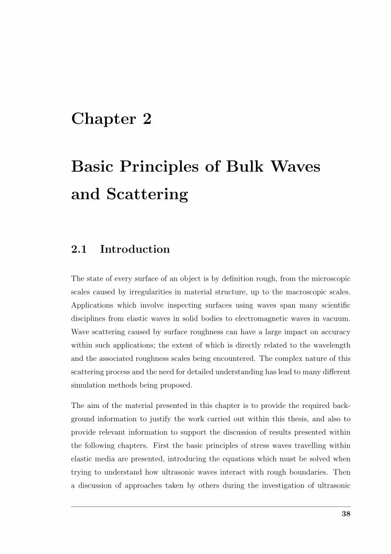
2.3 Rough surfaces with Gaussian height and length characteristics when
(a) σ=0.1mm (λ/16) and λ0=2.4mm (3λ/2), (b) σ=0.3mm (∼ λ/5)
and λ0=0.4mm (λ/4). . . . . . . . . . . . . . . . . . . . . . . . . . . . . 47
2.4 Scattered (i) coherent (ii) and diffuse (iii) components of the far field
amplitude from a rough defect measuring 6λ in length for a planar
incident scalar wave at 30○ when (a) σ = 0 and λ0 = ∞, (b) σ = λ/8
and λ0 = λ/2 (c) σ = λ/4 and λ0 = λ/2. . . . . . . . . . . . . . . . . . . . 49
3.1 Two dimensional scattering geometry . . . . . . . . . . . . . . . . . . . 54
10

LIST OF FIGURES
3.2 Diagram showing how the problem geometry of the DPSM simulation
is constructed, illustrating the naming convention of each of the Q
matrices and boundaries. . . . . . . . . . . . . . . . . . . . . . . . . . . . 56
3.3 Fresnel length of a planar rectangular transducer . . . . . . . . . . . . 61
3.4 Simplified crack geometries (a) 90○ angular crack used to demonstrate
multiple scattering and surface self shadowing (b) 90○ incidence on
planar crack used to compare diffracted signal amplitudes. . . . . . . 62
3.5 Scattered amplitude under normal plane wave incidence (a) 90○ con-
cave angled crack (b) 90○ incidence on planar crack . . . . . . . . . . . 62
3.6 Scattered signal at a distance of 5λ normal to the planar crack face
under normal incidence with a crack length of (a) 17λ (within near
field) (b) 2λ (within far field). Thinner lines show the Hilbert en-
velopes of each signal. . . . . . . . . . . . . . . . . . . . . . . . . . . . . 65
3.7 Time domain signals for all scattered angles around a planar crack
with a length of 10λ. (a) Results from DPSM simulation with r = 7λ.
(b) Results using Kirchhoff approximation with r = 7λ. (c) Percentage
difference in amplitude of the Hilbert envelope results from (a) and
(b). (d) Results from DPSM simulation with r = 45λ (e) Results
using Kirchhoff approximation with r = 45λ (f) Percentage difference
in amplitude of the Hilbert envelope results from (d) and (e). . . . . 66
3.8 Time domain signals for all scattered angles around a rough crack
with a length of 10λ, an RMS height of λ/10 and a correlation length
of λ/2. (a) Results from DPSM simulation with r = 7λ (b) Results
using Kirchhoff approximation with r = 7λ (c) Percentage difference
in amplitude of the Hilbert envelope results from (a) and (b). (d) Re-
sults from DPSM simulation with r = 45λ (e) Results using Kirchhoff
approximation with r = 45λ (f) Percentage difference in amplitude of
the Hilbert envelope results from (d) and (e). . . . . . . . . . . . . . . 67
11

LIST OF FIGURES
3.9 (a) Schematic of experimental setup. (b) Plan view of the final stage
of the machined sinusoidal surface. Areas within the dashed lines
indicate the approximate locations of the contact patches of each
waveguide. . . . . . . . . . . . . . . . . . . . . . . . . . . . . . . . . . . . 70
3.10 Simulated signals s12 obtained using the DPSM and FEM simulations
with an input pressure amplitude of 1, showing the unscaled reflected
scalar wave pulse from a sinusoidal surface with RMS heights of (a)
0.1mm, (b) 0.2mm and (c) 0.3mm. Similar results for signals s32 and
RMS heights of (d) 0.1mm, (e) 0.2mm and (f) 0.3mm. Dotted lines
show the Hilbert envelopes of each signal. . . . . . . . . . . . . . . . . 72
3.11 Experimental signals showing the reflected SH wave pulse from a one
dimensional sinusoidal surface with a surface wavelength of 4mm and
RMS heights of (a) 0.12mm, (b) 0.20mm and (c) 0.28mm. Simulated
signals obtained using the two dimensional scalar wave DPSM model
from the same surface with RMS heights of (d) 0.12mm, (e) 0.20mm
and (f) 0.28mm. Dotted lines show the Hilbert envelopes of each
signal. . . . . . . . . . . . . . . . . . . . . . . . . . . . . . . . . . . . . . . 73
3.12 (a) Diagram of paths taken by the surface skimming wave and back-
wall reflection from the transmitter to the receiver. (b) Experimental
signal taken when backwall was flat, illustrating the unwanted modes
travelling along the waveguides adding coherent noise which is on
average 22dB lower than the amplitude of the backwall reflection. . . 75
3.13 Comparison of the maximum envelope amplitude measured experi-
mentally and calculated using the two dimensional scalar wave DPSM
simulation for both waveguide pairs within the 3 waveguide array. Er-
ror bars represent the -22dB amplitude error that could be introduced
by unwanted modes travelling within the waveguides. . . . . . . . . . 75
3.14 Scattered field when a 2MHz plane wave with a velocity of 3260ms−1
is normally incident upon a sinusoidal backwall with an RMS height
of 0.1mm and a surface wavelength (λs) of (a) 0.5mm, (b) 2mm, (c)
8mm and (d) 50mm. . . . . . . . . . . . . . . . . . . . . . . . . . . . . . 77
12

LIST OF FIGURES
3.15 Average Fourier transforms of 5000 rough surfaces with the same
correlation lengths for various correlation length values, indicating
the length scales of features present within the surfaces. Amplitudes
are relative to the length scale with the largest contribution to the
average spatial frequency content. . . . . . . . . . . . . . . . . . . . . . 78
4.1 (a) Schematic of wall thickness sensor showing paths taken by surface
skimming wave and backwall reflection. (b) Simulated signals from a
flat backwall and a rough backwall when σ = 0.2mm and λ0 = 0.8mm
showing the surface skimming wave and backwall reflection which
would be received and used to calculate wall thickness. . . . . . . . . 82
4.2 Simulated scattered pulse shapes and surface profiles for three sur-
faces where σ = λ/8 and λ0 = λ illustrating examples of (a) high
ampltiude (b) low amplitude, and (c) similarity to flat backwall re-
sponse. Simulated Signals with the same σ value but λ0 = λ/2 showing
examples of (d) energy in signal tail, (e) stretched/offset pulse, and
(e) multiple pulses. Each signal is shown alongside the specific surface
from which it reflected. . . . . . . . . . . . . . . . . . . . . . . . . . . . . 85
4.3 Comparison of the median maximum amplitude of Hilbert envelope
of reflected pulses from surfaces with RMS heights up to 0.3mm (σ <
λ/5) and correlation lengths between 0.4mm and 2.4mm (λ/4 < λ0 <
2λ/3). . . . . . . . . . . . . . . . . . . . . . . . . . . . . . . . . . . . . . . 86
4.4 Example rough backwall simulated signal, showing the coherent com-
ponent calculated using 500 simulated signals and the diffuse compo-
nent. . . . . . . . . . . . . . . . . . . . . . . . . . . . . . . . . . . . . . . . 87
4.5 (a) Frequency spectra of coherent pulses reflected from rough surfaces
with correlation lengths of 0.8mm (λ0 = λ/2) and RMS heights of 0.06,
0.14, 0.22 and 0.3mm (σ = 0.04λ,0.09λ,0.14λand0.19λ). (b) Average
frequency spectra of diffuse components from the same surfaces. . . . 88
13

LIST OF FIGURES
4.6 (a) Peak frequencies in frequency spectra of coherent pulse and aver-
age frequency spectra of diffuse components for all RMS height values
(0.02 to 0.3mm in 0.02mm increments) and correlation length values
(0.4, 0.8, 1.6 and 2.4mm) investigated. (b) Amplitudes at peak fre-
quencies. . . . . . . . . . . . . . . . . . . . . . . . . . . . . . . . . . . . . 89
4.7 Box plots showing the statistical distribution of estimated wall thick-
ness values obtained for a 10mm thick wall with RMS heights ap-
proaching 0.3mm (σ < λ/5) and a correlation length of 0.8mm (λ0 =
λ/2 using (a) envelope peak detection (b) cross-correlation (c) thresh-
old first arrival with a -15dB threshold, and (d) threshold first arrival
with a -6dB threshold. . . . . . . . . . . . . . . . . . . . . . . . . . . . . 92
4.8 (a) Error in thickness estimation relative to incident wavelength when
using envelope peak TOF algorithm plotted against corresponding
correlation coefficient values for all 30000 simulated results. (b) Black
lines show percentile values for each section containing 10% of the
signals, percentiles are indicated by the value in the circle. Red line
shows the mean values of the correlation coefficient in each 10% sec-
tion. . . . . . . . . . . . . . . . . . . . . . . . . . . . . . . . . . . . . . . . 97
4.9 Uncertainty plot when using envelope peak detection TOF algorithm
for thickness evaluation and correlation coefficient as error metric.
Black lines represent the percentile values indicated in the circles.
Dotted lines represent an example of how the error bounds are esti-
mated for a correlation coefficient value of 0.95. . . . . . . . . . . . . . 97
4.10 Uncertainty plots for (a) envelope peak detection, (b) cross-correlation
and (c) threshold first arrival TOF algorithms when using (i) reflec-
tion amplitude, (ii) pulse width and (iii) correlation coefficient quality
metrics. The black lines from top to bottom in each plot represent
the 95th, 75th, 50th, 25th and 5th percentiles respectively. . . . . . . . . 98
14

LIST OF FIGURES
5.1 Geometry of reflecting inner surface and waveguide contact patches
for (a) two dimensional scattering and (b) three dimensional scatter-
ing. . . . . . . . . . . . . . . . . . . . . . . . . . . . . . . . . . . . . . . . 102
5.2 Diagram showing how the problem geometry of the DPSM simulation
is constructed in three dimensions, illustrating the naming convention
of each of the Q matrices and boundaries. . . . . . . . . . . . . . . . . . 104
5.3 a) Illustration of the displacement amplitude distribution as the pulse
travels along the waveguide. (b) Amplitude distribution of an SH0*
plane wave propagating within a 15mm thick semi-infinite plate as
calculated using Disperse. . . . . . . . . . . . . . . . . . . . . . . . . . . 105
5.4 (a) Change in reflected pulse shape from a flat surface as subdivided
section areas decrease. (b) Average absolute difference of amplitudes
within a 20dB bandwidth of the centre frequency as section area
decreases compared with original surface, also showing a comparison
of simulation time with that of original surface. . . . . . . . . . . . . . 107
5.5 (a) Plan view of the final stage of the rough surface machined with
RMS height of 0.3mm (σ ≈ λ/5) and a correlation length of 1.6mm
(λ0 = λ). Areas within the dotted lines indicate the approximate
positions of the contact patches of each waveguide within the array.
(b) Photograph of holding jig, array of three waveguides and the test
sample after machining, also showing detail view of machined rough
surface (inset). . . . . . . . . . . . . . . . . . . . . . . . . . . . . . . . . . 110
5.6 Experimental signals showing the reflected SH wave pulse from a
rough surface with a correlation length of 1.6mm (λ0 = λ) and RMS
heights of (a) 0.1mm, (b) 0.2mm and (c) 0.3mm. Simulated signals
obtained using the scalar wave DPSM model in three dimensions from
the same surface with RMS heights of (d) 0.1mm, (e) 0.2mm and (f)
0.3mm. Dotted lines show the Hilbert envelopes of each signal. . . . . 111
15

LIST OF FIGURES
5.7 Comparison of the maximum envelope amplitude measured experi-
mentally and calculated using the DPSM simulation for both waveg-
uide pairs within the 3 waveguide array. Error bars represent the
-22dB amplitude error that could be introduced by unwanted modes
travelling within the waveguides. . . . . . . . . . . . . . . . . . . . . . . 112
5.8 Simulated results showing the backwall reflection envelope maximum
amplitude when the array is incident upon different positions above
the rough surface with an RMS height of 0.1mm for (a) s12 and (b)
s32. (c) The difference in amplitude between neighboring positions
within the array. . . . . . . . . . . . . . . . . . . . . . . . . . . . . . . . . 114
5.9 Example backwall reflected signals from a rough surface with an
RMS height of 0.2mm (σ = λ/8) and a correlation length of o.8mm
(λ0 = λ/2) calculated using a (a) two dimensional simulation (b) three
dimensional simulation. . . . . . . . . . . . . . . . . . . . . . . . . . . . 116
5.10 (a) Schematic illustrating how correction factor is derived by aver-
aging a Gaussian distributed rough surface along one direction. (b)
Correction factor versus source length to correlation length ratio; can
be used for any RMS height, correlation length and source length
combination. . . . . . . . . . . . . . . . . . . . . . . . . . . . . . . . . . . 117
5.11 Comparison of scattered to coherent amplitude ratio of two dimen-
sional, three dimensional and two dimensional with correction sim-
ulated results when (a) ls = 2.5λ and λ0 = 0.25λ (b) ls = 5λ and
λ0 = 0.25λ (c) ls = 7.5λ and λ0 = 0.25λ (d) ls = 2.5λ and λ0 = 0.5λ
(e) ls = 5λ and λ0 = 0.5λ (f) ls = 7.5λ and λ0 = 0.5λ (h) ls = 2.5λ and
λ0 = λ (i) ls = 5λ and λ0 = λ (j) ls = 7.5λ and λ0 = λ (k) ls = 2.5λ and
λ0 = 1.5λ (l) ls = 5λ and λ0 = 1.5λ (m) ls = 7.5λ and λ0 = 1.5λ. . . . . . 119
16

LIST OF FIGURES
5.12 Box plots showing the statistical distribution of estimated wall thick-
ness values obtained for a 10mm thick wall with RMS heights ap-
proaching 0.3mm (σ < λ/5) and a correlation length of 0.8mm (λ0 =
λ/2 using (a) envelope peak detection (b) cross-correlation (c) thresh-
old first arrival with a -15dB threshold, and (d) threshold first arrival
with a -6dB threshold. Simulated signals were obtained using the
two dimensional DPSM simulation and corrected using ’2D to 3D’
correction factor for an assumed source length of 12mm. . . . . . . . 121
5.13 The values of the interquartile range for three dimensional, two di-
mensional and two dimensional with correction as RMS height in-
creases for (a) envelope peak detection, (b) cross-correlation and (c)
threshold first arrival with a threshold of -15dB. . . . . . . . . . . . . . 122
5.14 Uncertainty plot when using envelope peak detection TOF algorithm
for thickness evaluation and correlation coefficient as error metric.
Black lines represent the percentile values indicated in the circles
when ’2D to 3D’ correction is applied to results from the two dimen-
sional DPSM simulation. Red lines show the equivalent percentile
values for the same results without correction. . . . . . . . . . . . . . . 123
6.1 (a) Amplitude change of backwall reflection compared with flat back-
wall conditions. (b) Change in pulse width 15dB below peak ampli-
tude relative to pulse width under flat backwall conditions. Compar-
ison of simulated backwall reflection signals when the inner surface is
flat and has a FBH located directly beneath the wall thickness sensor
with a diameter of 3.2mm (2λ) and a depth of (c) 0.4mm (λ/4) and
(d) 3.2mm (2λ). Dashed lines represent the Hilbert envelopes of the
associated signals. . . . . . . . . . . . . . . . . . . . . . . . . . . . . . . . 130
6.2 Plan view showing the depth of conical pit during machining during
stage (a) 1 (max depth of 100µm) (b) 2 (max depth of 200µm) (c) 3
(max depth of 300µm) (d) 4 (max depth of 400µm) (e) 5 (max depth
of 500µm). (f) Isometric view of conical pit after the final stage of
machining. . . . . . . . . . . . . . . . . . . . . . . . . . . . . . . . . . . . 131
17

LIST OF FIGURES
6.3 Signal comparison when the backwall is flat and with the largest coni-
cal pit (stage 5) for (a) experimental results (b) simulated results. (c)
Comparison of amplitude change calculated using the DPSM simula-
tion and recorded using the thickness sensor for all defect geometries
machined during the experiment. . . . . . . . . . . . . . . . . . . . . . . 132
6.4 Signal comparison when the backwall is flat and with a 3mm diame-
ter FBH with a depth of 3mm directly below the thickness sensor for
(a) experimental results (b) simulated results. (c) Comparison of am-
plitude change calculated using the DPSM simulation and recorded
using the thickness sensor for all FBH depths. Error bars represent
the amplitude error that could be introduced by unwanted modes
travelling within the waveguides which are on average 22dB weaker
than the backwall reflection when the inner surface is flat. . . . . . . 134
6.5 Plan view of the depth of the machined surface directly below the
sensor at stage (a) 7 (b) 14 and (c) 20. . . . . . . . . . . . . . . . . . . 136
6.6 Signal comparison when the backwall is flat and the final stage of
corrosion machining (stage 20) for (a) experimental results (b) sim-
ulated results. (c) Comparison of amplitude change calculated using
the DPSM simulation and recorded using the thickness sensor for all
machined corrosion stages. Error bars represent the amplitude er-
ror that could be introduced by unwanted modes travelling within
the waveguides which are on average 22dB weaker than the backwall
reflection when the inner surface is flat. . . . . . . . . . . . . . . . . . . 137
6.7 Examples of single pits resulting from conditions of (a) uniform growth
(b) non-uniform growth. . . . . . . . . . . . . . . . . . . . . . . . . . . . 140
6.8 Example of a corroding backwall shown alongside the simulated pulse
reflected from the surface calculated using the DPSM for a mean wall
loss of (a) 0.07mm (b) 0.55mm (c) 0.79mm (d) 0.9mm (e) 0.97mm
and (f) 1mm. . . . . . . . . . . . . . . . . . . . . . . . . . . . . . . . . . 141
18

LIST OF FIGURES
6.9 (a) Comparison of estimated wall thickness trends for envelope peak
detection (EP), cross-correlation (XC) and threshold first arrival (FA)
TOF algorithm. A 15dB threshold was used for FA. Lines have
been included showing the actual minimum, maximum and mean
wall thickness of the surface calculated using the surface profiles. (b)
Comparison of linear regression lines and their associated COD val-
ues for each TOF algorithm. The data points show the wall thickness
estimates from which the linear regression lines have been calculated. 142
6.10 (a) COD values for all simulated results. (b) Corrosion gradient val-
ues for all simulated results, (c) for linear regression lines with COD
values greater than 0.9. (d) COD values for simulated results up to a
mean wall loss of 0.75mm. (e) Corrosion gradient values for simulated
results up to a mean wall loss of 0.75mm, (f) for linear regression lines
with COD values greater than 0.9. . . . . . . . . . . . . . . . . . . . . . 143
6.11 (a) Correlation coefficient of simulated signals as pitting corrosion
proceeds for example surface. (b) Average correlation coefficient and
RMS height as corrosion proceeds over 950 surfaces. . . . . . . . . . . 146
6.12 Correlation coefficient values for experimental signals reflecting from
a three dimensional Gaussian distributed rough surface with a corre-
lation length of 1.6mm (λ0 = λ) as RMS height increases. . . . . . . . 147
7.1 (a) Geometry considered for diffraction of a plane wave from a crack
tip when the incident angle θ is equal to the receiving angle. (b)
Diffracted SH wave amplitude when the observation distance (r) is
30mm and λ=1.6mm. The dashed line represents the typical signal
to noise ratio for standard equipment (-40dB). . . . . . . . . . . . . . . 153
7.2 (a) Array geometry considered showing the path analyzed during
TFM imaging. (b) Example TFM image calculated using simulated
signals. . . . . . . . . . . . . . . . . . . . . . . . . . . . . . . . . . . . . . . 154
7.3 Sketch showing the DPSM model geometry after the simplifying as-
sumption that the backwall acts as a perfect reflector . . . . . . . . . . 155
19

LIST OF FIGURES
7.4 (a) Estimated crack lengths for various sizes of array in a 30mm thick
plate containing a defect placed 10mm away from the array. (b) Error
in defect length estimation for a 5mm defect in a 30mm thick steel
plate due to the number of transducers within the array for various
defect positions. Results are based on simulated data from the DPSM
simulation . . . . . . . . . . . . . . . . . . . . . . . . . . . . . . . . . . . . 156
7.5 (a) Schematic of the SH waveguide array and transmit-receive equip-
ment (b) photo of the prototype waveguide array coupled to a 30mm
thick steel plate with a 5mm notch . . . . . . . . . . . . . . . . . . . . . 158
7.6 Comparison of experimental and simulated results for a 5mm notch
in a 30mm thick steel plate, (a.i) experimental pitch-catch signals for
transmitting transducer number 8. (a.ii) Image using experimental
data. (b.i) Simulated pitch-catch signals for transmitting transducer
number 8. (b.ii) Image using simulated data. . . . . . . . . . . . . . . . 158
7.7 Images processed from data acquired when the SH array was clamped
to a 30mm thick steel plate containing (a.i) a 5mm deep notch, (b.i)
a 10mm deep notch, (c.i) a 15mm deep notch. (a.ii), (b.ii) and (c.ii)
show the corresponding -6dB contour plots. (dB values are relative
to the maximum values in the image, all notches were 0.3mm wide). . 159
7.8 (a) Photograph of the experimental setup showing the array and fur-
nace. (b) Histogram of estimated notch lengths showing distribution
throughout experiment. (c) Calculated wavespeed throughout exper-
iment. (d) Average amplitude change of first backwall reflection of
all pitch-catch signals throughout experiment relative to initial ampli-
tude. (e) Estimated notch length derived from -6dB contour around
defect image. . . . . . . . . . . . . . . . . . . . . . . . . . . . . . . . . . . 161
7.9 (a) Photograph of the final array installation (b) Latest crack image,
calculated using data taken in January 2012 . . . . . . . . . . . . . . . 163
7.10 Schematic of array geometry incident upon an area of hydrogen attack
showing two possible ray paths through the area of degradation. . . . 167
20

LIST OF FIGURES
7.11 Relationship between ultrasonic shear wave velocity and temperature
of mild steel test specimen. . . . . . . . . . . . . . . . . . . . . . . . . . . 169
7.12 (a) Steady state heat conduction simulated temperature distribution.
Reconstruction of temperature distribution using (b) Kaczmarz algo-
rithm (c) assumed distribution method. . . . . . . . . . . . . . . . . . . 170
7.13 (a) Schematic of heating arrangement to produce a two dimensional
temperature distribution below the array. (b) Photograph of experi-
mental setup. . . . . . . . . . . . . . . . . . . . . . . . . . . . . . . . . . . 172
7.14 Reconstructions of temperature distribution at the end of the exper-
iment using (a) Kaczmarz algorithm and (b) the assumed distribu-
tion method for (i) centralised heat source and (ii) 10mm offset heat
source. The array is located along the top of the images. . . . . . . . 173
8.1 (a) Schematic of simple simulated case. Simulated signals showing
horizontal displacement (u1) and vertical displacement (u2) produced
by the elastic DPSM simulation and the two dimensional plane strain
FEM simulation using a 2MHz input Hanning windowed toneburst
point load at an observation point where (b) x1 = x2 =0.75mm, (b)
x1 = x2 =1.65mm and (c) x1 = x2 =2.60mm. . . . . . . . . . . . . . . . . 182
8.2 Box plots showing the statistical distribution of estimated wall thick-
ness values obtained using the two dimensional DPSM simulation for
a 10mm thick wall with RMS heights approaching 0.3mm (σ < λ/5)
and a correlation length of 0.4mm (λ0 = λ/4 using (a) envelope peak
detection (b) cross-correlation (c) threshold first arrival with a -15dB
threshold, and (d) threshold first arrival with a -6dB threshold. . . . 184
21

LIST OF FIGURES
8.3 Box plots showing the statistical distribution of estimated wall thick-
ness values obtained using the two dimensional DPSM simulation for
a 10mm thick wall with RMS heights approaching 0.3mm (σ < λ/5)
and a correlation length of 0.8mm (λ0 = λ/2 using (a) envelope peak
detection (b) cross-correlation (c) threshold first arrival with a -15dB
threshold, and (d) threshold first arrival with a -6dB threshold. . . . 185
8.4 Box plots showing the statistical distribution of estimated wall thick-
ness values obtained using the two dimensional DPSM simulation for
a 10mm thick wall with RMS heights approaching 0.3mm (σ < λ/5)
and a correlation length of 1.6mm (λ0 = λ using (a) envelope peak
detection (b) cross-correlation (c) threshold first arrival with a -15dB
threshold, and (d) threshold first arrival with a -6dB threshold. . . . 186
8.5 Box plots showing the statistical distribution of estimated wall thick-
ness values obtained using the two dimensional DPSM simulation for
a 10mm thick wall with RMS heights approaching 0.3mm (σ < λ/5)
and a correlation length of 2.4mm (λ0 = 3λ/2 using (a) envelope peak
detection (b) cross-correlation (c) threshold first arrival with a -15dB
threshold, and (d) threshold first arrival with a -6dB threshold. . . . 187
8.6 Box plots showing the statistical distribution of estimated wall thick-
ness values obtained using the two dimensional DPSM simulation
with ’2D to 3D’ correction and an assumed source length of 12mm
for a 10mm thick wall with RMS heights approaching 0.3mm (σ < λ/5)
and a correlation length of 0.4mm (λ0 = λ/4 using (a) envelope peak
detection (b) cross-correlation (c) threshold first arrival with a -15dB
threshold, and (d) threshold first arrival with a -6dB threshold. . . . 188
22

LIST OF FIGURES
8.7 Box plots showing the statistical distribution of estimated wall thick-
ness values obtained using the two dimensional DPSM simulation
with ’2D to 3D’ correction and an assumed source length of 12mm
for a 10mm thick wall with RMS heights approaching 0.3mm (σ < λ/5)
and a correlation length of 0.8mm (λ0 = λ/2 using (a) envelope peak
detection (b) cross-correlation (c) threshold first arrival with a -15dB
threshold, and (d) threshold first arrival with a -6dB threshold. . . . 189
8.8 Box plots showing the statistical distribution of estimated wall thick-
ness values obtained using the two dimensional DPSM simulation
with ’2D to 3D’ correction and an assumed source length of 12mm
for a 10mm thick wall with RMS heights approaching 0.3mm (σ < λ/5)
and a correlation length of 1.6mm (λ0 = λ using (a) envelope peak
detection (b) cross-correlation (c) threshold first arrival with a -15dB
threshold, and (d) threshold first arrival with a -6dB threshold. . . . 190
23

Nomenclature
α ’2D to 3D’ correction factor
γ Lame’s first parameter
δij Kronecker delta function
εij Strain tensor
θ Incident / reflected angle
λ Wavelength
λ0 Correlation length
λs Wavelength of sinusoidal surface
µ Shear modulus (Lame’s second parameter)
ρ Density
ρij Correlation coefficient between signals i and j
σ RMS height
σ RMS height of average surface
σij Stress tensor
σd Standard deviation
φ Scalar potential
ψ Acoustic pressure
ω Angular frequency
a Point source separation
aw Waveguide separation
A Amplitude
c Wave speed
C Autocorrelation function
Cijkl Elasticity tensor
di, d(x) Random number deviation from population mean
e Unit vector
Fi Body force per unit volume
G Green’s function
hi, h(x) Surface deviation from mean plane
h Vector potential
i Imaginary variable (√−1)
Continued on next page. . .
24

– Continued from previous page
I(i, j) Image amplitude at pixel (i, j)
k Wavenumber
LF Fresnel length
Lc Crack length
n Unit normal vector
p probability density function
r Radial vector
r Radial distance
rs Point source boundary offset
R Reflection coefficient
sij signal received on element i when transmitted from element j
S Closed surface
t Time
T Wall thickness
u Displacement vector
wi,w(x) Weights of correlation function
Subscripts
inc Incident field
L Longitudinal waves
ref Reference field
sct Scattered field
T Shear (transverse) waves
25

Abbreviations
BIE Boundary integral equation
COD Coefficient of determination
DPSM Distributed point source method
DSP Digital signal processing
EDM Electric discharge machining
EP Envelope peak detection
FA First arrival
FEM Finite element method
FFT Fast Fourier transform
FMC Full matrix capture
GMRes Generalised minimum residual method
IFFT Inverse fast Fourier transform
IQR Interquartile range
NAC Naphthenic acid corrosion
RMS Root mean squared
SC Sulphidic corrosion
SH Shear horizontal
TFM Total focussing method
TOF Time of flight
TOFD Time of flight diffraction
XC Cross-correlation
26

Chapter 1
Introduction
1.1 Motivation
Ultrasound refers to acoustic and elastic waves with frequencies higher than the
audible range of human hearing, typically ranging from 20kHz to several GHz. It is
used in a wide range of medical and engineering applications from real-time three
dimensional imaging of structures within the human body [1] to metal and poly-
mer welding [2]. It is this versatility which make it such an important research topic
within many scientific disciplines. The focus of the work presented within this thesis
will be specifically on its use in the nondestructive evaluation (NDE) of engineering
structures, a critical research area which has grown rapidly over the last half cen-
tury, providing engineers with increasingly rapid, accurate, sensitive and economical
means of inspecting structures.
Some of the earliest work utilizing ultrasonic waves for nondestructive testing of
engineering structures was carried out during World War II by Firestone for detect-
ing cracks in tank armour plating [3]. Called the ’Supersonic Reflectoscope’ [4], the
device applied a high frequency voltage to a quartz crystal to enact a small volume
change. When coupled to a test specimen using a thin oil film, mechanical waves
were transmitted into the specimen which would subsequently reflect from flaws and
boundaries. By transmitting bursts of ultrasonic energy into the metallic structure
and then displaying the returning echoes on an oscilloscope, an assessment could
27

1. Introduction
be made about whether internal flaws were present or not. This was the earliest
implementation of ultrasonic pulse-echo inspection and the fundamental principles
of NDE devices using piezoelectric crystals remain largely unchanged to this day.
What has changed dramatically however, is the sensitivity of the equipment and the
analysis of the data.
The improvement of ultrasonic NDE equipment and its ability to detect smaller
flaws, coupled with the development of fracture mechanics as an engineering disci-
pline in the early 1970s lead to the emergence of quantitative nondestructive eval-
uation (QNDE) as an increasingly important area of research [5]. No longer were
inspections aimed solely at detecting whether a defect was present or not, damage
tolerant design meant that if a defect could be detected and quantitatively char-
acterised in terms of length, size or severity, stress analysts could make informed
decisions whether a structure was within safe operational limits. This is particularly
important for in-service inspection of structures whose failure could cause consider-
able financial burden or loss of human life; for example aircraft, nuclear reactors and
ageing civil infrastructure such as bridges, steam power plants and petrochemical
processing plants.
Many of the challenges faced within the power generation industry are shared by
refineries and chemical processing plants around the world; most notably high oper-
ating temperatures, aging equipment, high replacement costs and the requirement
for greater efficiency in the face of increasing safety and reliability concerns [6]. As
an example, within the UK, deregulation of the electricity market around 25 years
ago has lead to power plants, which were originally designed for base load conditions,
to be cycled much more rapidly to meet the demands of an increasingly competi-
tive and fluctuating energy market. Known as two-shifting, this mode of operation
subjects plants which have already surpassed their deign lives to operate extensively
within the regimes where material fatigue and creep damage are of major concern
[7, 8]. Failure mechanisms associated with the high temperature operating condi-
tions experienced within power plant and refinery environments arise in a number
of ways including creep, hydrogen attack, oxidation, thermal fatigue, low cycle fa-
tigue and thermal shock [9]. Additional to these, there are also damage inducing
mechanisms which work over a wider range of temperatures including atmospheric,
28

1. Introduction
galvanic, acidic, biological and erosion corrosion [6, 10]. Oftentimes a number of
these mechanisms occur in parallel, causing a multitude of defect morphologies in-
cluding crevices, cracks, intergranular porosity, pitting and general corrosion causing
pipe or pressure vessel wall thickness loss [10].
In an ideal world each inspection method would be tailored precisely to the defect
morphology it is designed to detect and monitor in order to extract the maximum
sensitivity from the equipment. However, because of the wide range of corrosion
mechanisms at work within such environments, it is not always clear what morphol-
ogy should be expected. As such, ultrasonic wall thickness measurement has become
the most widely used NDE technique within the power generation and petrochemical
industries as it is robust enough to provide quantitative and reliable measurements
over a wide range of corrosion conditions. An example where such data is of great
value is in estimating the remaining life of refinery furnace tubing which is coming to
the end of its life and suspected of imminent creep rupture. Moss et al [11] describe
a method of estimating the remaining life using material properties, temperature
and wall thinning rate as inputs; the sensitivity of which is directly related to the
accuracy of each of these measures. However, the difficulty in measuring the wall
thickness of the in-service furnace reported in this study reflects the primary chal-
lenge faced when applying any NDE technique within such hostile environments:
standard equipment cannot withstand high operating temperatures. For ultrasonic
equipment, the limiting factor is often the Curie temperature (Tc) of the piezoelec-
tric material, beyond which crystal depolarization occurs rendering the transducer
useless. This generally limits the use of standard lead zirconate titanate (PZT) ce-
ramics to a maximum temperature of approximately 200○C [12], well below that of
the operational temperatures of power plants and refinery furnaces which tend to
operate between 300 and 500○C.
There are two main solutions to this problem: non-contact solutions where all hard-
ware is physically separated from the undesirable effects of temperature, or contact
solutions which either strive to use piezoelectric materials with higher Tc values or
introduce a mechanical connection between the PZT crystal and the workpiece in
order to transmit ultrasound. Non-contact solutions cover a range of techniques
[13]. Since the late 1970s electromagnetic acoustic transducers (EMATs) have been
29

1. Introduction
developed and used in various applications including high accuracy thickness gaug-
ing [14]. However, the requirement for a low separation distance to the workpiece
would still make them vulnerable to high temperatures, particularly those utilising
permanent magnets which themselves have a maximum Tc in the region of 300○C.
Lasers can also be used to generate ultrasonic waves by transient surface heating,
as well as detect them through interferometry. Kruger et al demonstrate this by
measuring wall thicknesses up to 100mm and 1250○C [15]; however, such systems
are generally considered as less sensitive than equivalent piezoelectric devices, and
are certainly much more expensive making them unsuitable for mass deployment
within plant environments. Theoretically air coupled ultrasonic transducers could
also be used to inspect high temperature components; however, the very large dif-
ference in specific acoustic impedances of solids and gases makes transmission and
detection through metallic components difficult [16]. Achieving sufficient tempera-
ture isolation from very high temperature structures over short distances also make
the approach unsuited to plant environments.
Solutions where a mechanical connection exists between the piezoelectric crystal
come in two forms; those which alter the piezoelectric material to operate at high
temperature or those which use a thermally isolating buffer rod. Kirk et al [17]
focus on the former and describe the development of transducers constructed using
lithium niobate (LiNbO3) which has a Tc =1210○C. Early development focused on
replicating ambient temperature designs; however, this approach led to unreliable
and expensive transducers since the structure of the piezoelectric, backing block and
front face layer became overcomplicated in order for the probes to be able to scan.
To overcome this, monolithic arrays with far simpler structures were developed and
tested with some success up to approximately 450○C [18, 19]; however, they suffer
from complicated and lengthy bonding processes which failed under thermal cycling.
The use of many different materials with varying thermal expansion coefficients
within one transducer also leads to complications during construction and use at high
temperature. Other major limitations to the commercial viability of transducers
using LiNbO3 are its low electromechanical coupling coefficient and its tendency
to crack during cooling. Schmarje et al [20, 21] describes the development of 1-3
connectivity LiNbO3 composites as a way of improving this by introducing a flexible
matrix material. It was found that the electromechanical coupling coefficient of the
30

1. Introduction
composite was roughly double that of crystalline LiNbO3 and that the material
was more stable during thermal cycling; however, a reliable coupling method under
fluctuating temperature conditions was still lacking. Kelly et al [22] report on a
permanently installable TOFD system designed to monitor thermal fatigue crack
growth which is constructed using modified sodium bismuth titanate (MNBT) for
operation up to 600○C. Diffracted signal amplitudes measured using the probe on
an EDM notch were found to be barely visible above the noise floor making crack
length estimation unreliable, if not impossible.
Thermal isolation of conventional PZTs using buffer rods, also known as delay lines
or waveguides, is an established method of producing ultrasonic transducers ca-
pable of measuring physical quantities within high temperature environments in-
cluding fluid flow [23], component wall thickness for corrosion and crack detection
[24–27] and simultaneous measurement of temperature and viscosity [28]. This sim-
ple method removes the need for matching thermal expansion coefficients of the
transducer and specimen materials; however, it does create the need for a strong
and often permanent coupling between the two since acoustic impedance matching
coupling mediums such as gel can only be used at temperatures up to approxi-
mately 400○C. Cegla [29] describes the development of a waveguide transducer that
transmits and receives shear horizontal (SH) waves and investigates the effect that
different coupling methods have on the signal quality for thickness gauging purposes
in pulse-echo and pitch-catch configurations. Results showed that a welded contact
caused spurious signal reflections at the junction between the waveguide and the
component introducing large amounts of coherent noise into the signals. Silver sol-
dered contacts were found to perform better but had little signal consistency, even
though the same process was carried out for each contact. Dry coupled contacts
were found to perform the best, showing good consistency and little signal degra-
dation at high temperatures and during thermal cycling, provided enough pressure
was applied at the contact.
This waveguide transducer, whose working principles are described in detail in [26],
was subsequently developed into a commercially available wall thickness monitoring
sensor [30]. It operates by transmitting a 2MHz 5 cycle Hanning windowed toneburst
into the high temperature environment via one waveguide, and then receiving the
31

1. Introduction
pulse which has reflected from the inner surface of the wall along the other waveg-
uide. An estimate of the wall thickness can subsequently be made by calculating
the time of flight (TOF) of the pulse within the component wall and using it in con-
junction with the ultrasonic wavespeed within the component material (see section
4.3.1). Thickness measurements and full waveforms are then relayed to operators
using wireless data connectivity, very well suited to the complicated infrastructure
encountered within industrial plant environments where access for inspection is dif-
ficult, dangerous and costly. The ability to survive operating temperatures in excess
of 550○C and transmit data autonomously represent the major advantages of the
sensor; continual wall thickness monitoring at a single location can be carried out,
improving dramatically on the repeatability and data content previously offered by
periodic inspections which could only be carried out during plant shut down.
The sensor is now established as an industry leader for providing wall thickness
monitoring data within high temperature environments, and as such has been de-
ployed in refineries around the world, providing data from many locations subject
to a wide variety of corrosive conditions. By inspection of the waveforms recorded
by many of the sensors it has become clear that a better understanding of the data
is required. If corrosion proceeds in a general manner with approximately uniform
wall loss in the vicinity of the sensor, little change in reflected signal shape would
occur, it would simply be recorded earlier in time signifying a distance change to the
inner surface. However, as described previously, corrosion can proceed through a
multitude of different defect morphologies such as localised pitting causing isolated
defects and areas or surface roughness. The changes these cause to the shape of the
inner surface have a direct impact on the shape of the pulse which is received, and
depending on how the TOF is extracted from the waveform, corrosion at the inner
surface can have a potentially large impact on the error associated with the final
wall thickness estimate. A particularly extreme example of an unexpected thickness
trend is shown in figure 1.1 (c), alongside example signals used to calculate the wall
thickness. The first pulse seen in Figs. 1.1 (a) and (b) is the surface skimming wave
travelling directly from the transmitter to the receiver and the second pulse is the
reflection from the inner surface (see Fig. ??). The thickness was calculated using
recorded waveforms using an envelope peak detection TOF algorithm (see section
4.3.1). It is clear that the shape of the reflection from the inner surface (or backwall
32

1. Introduction
185 190 195 200 205 210 215 220 225 230 235-0.8
-0.6
-0.4
-0.2
0
0.2
0.4
0.6
0.8
1
3252 10-10-30 thickness = 0.43 in
time, usec
norm
alis
ed a
mp.
185 190 195 200 205 210 215 220 225 230 235-0.8
-0.6
-0.4
-0.2
0
0.2
0.4
0.6
0.8
1
3252 10-11-13 thickness = 0.404 in
time, usec
norm
alis
ed a
mp.
(a) (b)
(c)
Time
Thic
knes
s (i
n)
Figure 1.1: Ultrasonic signals recorded at a location showing an unexpected thicknesstrend in (a) September and (b) November. The first pulse seen within the recordedwaveforms is the surface skimming wave and the second pulse is the reflection from theinner surface. (c) Thickness trend as calculated using the recorded waveforms using anenvelope peak detection TOF algorithm. Reproduced under permission from PermasenseLtd.
reflection) changes between the dates shown which causes the calculated thickness
to increase rapidly by 0.13mm at the end of October, then decrease by 0.7mm only
to recover back to a steady wall thickness value of 10.7mm in December, 0.13mm
below the value indicated in October. It is expected that corrosion induced surface
roughness is the primary factor in determining these apparent errors in thickness
measurement.
Although this is not an ideal situation in terms of thickness measurement accuracy
based on the TOF algorithm used, it also presents an opportunity; if a relationship
between roughness severity / defect size and pulse shape change exists, extra infor-
mation about the nature of corrosion occurring within the pipe or pressure vessel
could be extracted. To derive such a relationship, a simulated study would provide
the ideal platform on which to mount an investigation. However, great challenges
still exist when trying to accurately and efficiently simulate how ultrasound reflects
33

1. Introduction
from rough surfaces, particularly for three dimensional geometries. Therefore one
major objective of this thesis is to overcome these challenges and implement a sim-
ulation technique which can offer the required accuracy and efficiency to carry out
such an investigation in both two dimensional and three dimensional geometries. In
doing so, not only will the explanation of odd trends which are sometimes observed
in field data be a priority; mitigating such trends through alternative signal process-
ing techniques will be of primary importance, as well as distinguishing whether there
is a way of quantitatively extracting an estimate of the shape of the inner surface
based on the shape change of the reflected pulse. Such processing techniques are
not possible during probe scanning inspection because much larger signal variability
reduces sensitivity to small pulse shape changes, offering additional opportunities
for detailed data analysis when using permanently installed sensors as opposed to
data acquired during probe scanning.
As discussed previously, it is not only wall thickness loss which is of concern within
the high temperature environments experienced within the power generation and
petrochemical industries. Thermal fatigue cracks and bulk material degradation
through the action of corrosion mechanisms such as hydrogen attack can also cause
catastrophic failure. Therefore, another objective is to explore alternative ways of
utilising the waveguide transducers to offer means of monitoring structural degra-
dation processes other than wall thickness loss.
1.2 Outline of thesis
This thesis investigates how ultrasonic waves scatter from rough boundaries between
materials with very different acoustic impedances. A semi-analytical mesh-free sim-
ulation method called the distributed point source method (DPSM) is applied to
the problem and used in conjunction with the scalar wave approximation for SH
wave scattering in order to produce a simulation technique which provides a better
compromise between accuracy and efficiency than any other technique currently of-
fers. The simulation is described in detail and verification of results is carried out
using the finite element method (FEM) and experimental investigations for two di-
mensional and three dimensional geometries. Although focus is paid predominantly
34

1. Introduction
to the application of wall thickness monitoring and the effect corrosion can have on
the recorded signals, alternative usage of the high temperature waveguide transduc-
ers for monitoring other defect morphologies is also discussed and experimentally
verified.
Chapter 2 introduces the governing equations of mechanical wave propagation within
solid media, providing a general background to ultrasonic wave interaction along
a boundary between two media. The specific problem of scattering along rough
boundaries is then explored by reviewing the most commonly implemented tech-
niques appearing within literature today, describing the different approaches and
the challenges faced during selection and implementation. The numerical genera-
tion of rough surfaces with Gaussian distributed height and length characteristics is
described in detail since they are used throughout the thesis to approximate surfaces
which could be expected under the corrosive conditions considered. The different
contributions within the scattered field from coherent and diffuse sources is then
introduced to make the terminology used in the rest of the thesis clear.
The scalar wave DPSM is described in detail in Chapter 3, using the simplified
two dimensional geometry of a sinusoidal surface for simulation validation using the
FEM, and experimental verification using the waveguide transducers. A detailed
comparison to classical Kirchhoff theory is also carried out in order to illustrate the
strength of the DPSM over the most commonly implemented technique found in
literature. Both monochromatic and time domain simulated cases are considered,
showing that although the Kirchhoff approximation ignores phenomena such as mul-
tiple scattering, surface self shadowing and tip diffraction, it is the far-field assump-
tion which makes it particularly unsuited to simulating scattering from compara-
tively large rough surfaces. The spatial frequency content of Gaussian distributed
rough surfaces is also shown in order to assess the limits of roughness which are to
be considered within this thesis.
The simulation is then applied to the practical problem of wall thickness monitor-
ing in Chapter 4, with the primary goal of assessing how different TOF algorithms
perform when confronted by signals reflecting from two dimensional rough surfaces.
Three commonly used digital signal processing techniques for calculating TOF are
tested: envelope peak detection, cross-correlation and threshold first arrival, indicat-
35

1. Introduction
ing that under low roughness conditions cross-correlation shows the lowest variability
and that threshold first arrival is the most stable under increasingly rough condi-
tions. A number of signal quality metrics are also introduced as a way of estimating
the most likely error in wall thickness measurement associated with a change in
signal shape.
In order to gain a sufficient number of simulated signals to carry out the investi-
gations in Chapter 4, the two dimensional geometry assumption had to be made,
approximating a real rough surface as a corrugated (or furrowed) boundary, echo-
ing the approach of a vast majority of literature. The shortcoming this assumption
introduces to simulated data is tackled in Chapter 5 by applying the DPSM to a
three dimensional rough surface geometry. Particular attention is paid to improv-
ing efficiency to ensure a simulation which can be completed within a reasonable
timescale. Because of the comparatively large length scales of the scattering geom-
etry being considered, simulation validation can only be carried out by comparison
to experimental results, showing good agreement at two different locations above a
surface with increasing roughness. Comparison between two dimensional and three
dimensional simulated results is subsequently carried out, leading to the proposal of
a correction factor capable of converting two dimensional results to more closely re-
semble those from a three dimensional rough surface given the transducer geometry
and statistical properties of the surface being considered.
Chapter 6 focusses on pitted surfaces which cannot be characterized using Gaussian
height and length scales, in particular use is made of the flat bottomed hole geome-
try as a simple approximation of a pitted defect. First, the limits of detection of the
sensor are explored using singular localised defects of very small and large length
scales; the small being manufactured at a micron scale using a micromachining laser
and the large using a milling machine. Comparison is made to the DPSM simula-
tion, again showing agreement within expected experimental error bounds. Then a
simulated corrosion model is implemented to more closely approximate how rough
and pitted surfaces might evolve over time, and the associated error in corrosion
rate is assessed for each TOF algorithm. Similar conclusions are drawn as those
for Gaussian distributed rough surfaces in terms of algorithm stability and the diffi-
culty of performing inverse scattering with the limited data available within a single
36

1. Introduction
ultrasonic signal.
The focus of Chapter 7 is therefore exploring applications where the extra infor-
mation provided by multiple waveguide transducers could be exploited. Two ap-
plications are described in detail which use array geometries to monitor structural
degradation mechanisms other than wall thickness loss. The first uses the multi
total focussing method (TFM) to create an image of thermal fatigue cracks. Ex-
perimental validation on EDM notches shows that it performs well on defects of
varying lengths and is able to survive temperature fluctuations greater than 500○C
for a period of 6 months. This culminated in an opportunity to install a prototype
on an operational steam power plant. The second application is the detection and
monitoring of hydrogen attack through ultrasonic velocity reconstruction in the area
below an array. A proof of concept experimental study was carried out using a tran-
sient two dimensional temperature distribution to assess whether the small changes
in velocity expected during such bulk material degradation could be detected. Two
imaging algorithms are applied, the Kaczmarz algorithm and the assumed distribu-
tion technique, both of which were found capable of detecting small velocity changes,
providing estimates of distribution position and extent.
Chapter 8 summarizes the conclusions of the thesis. Suggestions of areas for future
work are also provided.
37
Chapter 2
Basic Principles of Bulk Waves
and Scattering
2.1 Introduction
The state of every surface of an object is by definition rough, from the microscopic
scales caused by irregularities in material structure, up to the macroscopic scales.
Applications which involve inspecting surfaces using waves span many scientific
disciplines from elastic waves in solid bodies to electromagnetic waves in vacuum.
Wave scattering caused by surface roughness can have a large impact on accuracy
within such applications; the extent of which is directly related to the wavelength
and the associated roughness scales being encountered. The complex nature of this
scattering process and the need for detailed understanding has lead to many different
simulation methods being proposed.
The aim of the material presented in this chapter is to provide the required back-
ground information to justify the work carried out within this thesis, and also to
provide relevant information to support the discussion of results presented within
the following chapters. First the basic principles of stress waves travelling within
elastic media are presented, introducing the equations which must be solved when
trying to understand how ultrasonic waves interact with rough boundaries. Then
a discussion of approaches taken by others during the investigation of ultrasonic
38

2. Basic Principles of Bulk Waves and Scattering
wave scattering from rough boundaries is carried out, paying particular attention to
the issues still faced in solving this very complex problem. Finally, the form of the
rough surfaces predominantly being investigated within this thesis will be derived
in detail. Much of the relevant literature has been described in my papers [31] and
[32], therefore relevant excerpts have been included in the following sections.
2.2 Wave Propagation in Bulk Media
The motion of stress waves within solid media has been extensively studied and
covered by many authors. For this reason, only a brief introduction will be provided
at this point (see [33–35] for more information). In a Cartesian coordinate system
and using tensor notation, the equation of linear momentum is given by
σij,j + Fi = ρui (2.1)
Where σij is the stress tensor, Fi is the body force per unit volume, ρ is the density
of the medium and u represents particle displacement. The constitutive law can be
used to relate stress and particle displacement which for any linear material can be
written as
σij = Cijklεkl (2.2)
Where Cijkl is the elasticity tensor which contains material constants and εkl is the
strain tensor in the solid. If the material can be assumed isotropic Hooke’s law is
given by
σij = γεkkδij + 2µεij (2.3)
Where γ and µ are the Lame constant of the material and δij is the Kronecker delta
function. For small deformation gradients, strain can be defined using the Cauchy
strain tensor
εij =1
2(ui,j + uj,i) (2.4)
Naviers equation of motion is then obtained by substituting equations 2.3 and 2.4
into equation 2.1, assuming a homogeneous medium with uniform temperature in
39

2. Basic Principles of Bulk Waves and Scattering
the absence of body forces.
(γ + µ)uj,ij + µui,jj = ρui (2.5)
If we take the divergence of equation 2.5, we find that dilatational (longitudinal)
motion must satisfy the equation
φ = c2Lφ,ii (2.6)
Where φ is a scalar potential and cL is the longitudinal wave speed defined by
cL =
√γ + 2µ
ρ(2.7)
Similarly if we take the curl of equation 2.5, we find rotational (shear) motion must
satisfy the equation
h = c2Thi,jj (2.8)
Where h is a vector potential and cT is the shear wave speed defined by
cT =
õ
ρ(2.9)
Therefore, wave motion as described by equation 2.5 can be broken into two con-
stituents that propagate at different velocities independent from one another within
unbounded media. The displacement vector at any point within a field can thus be
described as a summation of dilatational and rotational components.
u = ∇φ +∇ × h (2.10)
Equation 2.10, written in vector notation, is known as the Helmholtz decompo-
sition of the displacement vector. Coupling between wave modes only occurs at
the boundaries between two different materials which can lead to mode conversion
during reflection and refraction. In the simplest case of normal beam incidence,
some of the energy will be reflected back into the medium from which it originated
and some will be transmitted into the second medium. This leads to the definition
of the normal beam incidence reflection coefficient which can be used to calculate
40

2. Basic Principles of Bulk Waves and Scattering
the amplitude change for an incident wave traveling from medium 1 to 2 which is
subsequently reflected at the boundary.
R =ρ2c2 − ρ1c1ρ1c1 + ρ2c2
(2.11)
This simple analysis only holds when the incident wave is perpendicular to the
boundary, approaching from an angle can give rise to reflection, refraction and mode
conversion. Snells law, most commonly associated with optical light waves, can be
used to describe reflection and refraction angles of the incident waveform. However,
unlike electromagnetic waves or waves traveling in fluids, solid materials can sustain
waves with both longitudinal and shear components (see equation 2.10). This leads
to mode conversion where longitudinal waves incident at a boundary can give rise
to reflected and refracted shear waves and vice versa. This phenomenon can be
visualized as a wave vector reaching a boundary at an angle. Considered on its own,
this vector will give rise to a complicated wave field; however, it can be split into a
normal component responsible for longitudinal wave propagation and a tangential
component responsible for shear wave propagation. Snells law can still be used to
calculate refracted angles for each wave type, ensuring the correct wave velocities
are used (see pgs 44-49 of [34]). Figure 2.1 illustrates the polarization directions of
the displacements which give rise to each type of reflected or refracted wave.
An important point to note is that in this context, shear waves refer to shear verti-
cal waves which are polarized in the plane of wave propagation and displacements
associated with shear horizontal (SH) waves occur perpendicular to this plane. Kino
(pg 100 of [35]) highlights the case of SH wave reflection or refraction at a boundary
which has a constant cross-sectional shape perpendicular to the plane of propa-
gation as the only case where waves traveling within solids do not undergo mode
conversion. No energy is lost as other modes meaning that the elastodynamic waves
can be modelled as acoustic waves with a velocity equal to that of the SH wave.
This is a powerful simplification which is strictly only valid when dealing with two
dimensional reflection and refraction of SH waves which are polarized out of the
plane; however, it will be the starting assumption for the modelling of the three
dimensional situations considered in this thesis and its validity will be investigated
by comparison to experimental results.
41

2. Basic Principles of Bulk Waves and Scattering
SH SVL
Boundary
Medium 1
Medium 2
x
y
z
Figure 2.1: Polarization direction of displacements giving rise to longitudinal (L), shearvertical (SV) and shear horizontal (SH) waves.
2.3 Existing Techniques for Modeling Scattering
at Rough Interfaces
In 1963 Uretsky described the reflection of plane waves from a sinusoidal boundary
as a ’marvelously complex problem’ [36]. This complexity has lead to many different
models being proposed; what follows is a brief review of the literature (see for exam-
ple [37–41] for more information). All scattering models are essentially attempting
to solve the Helmholtz scattering integral over a closed surface S, which gives the
total field ψ at a point r′ away from the surface [42].
ψ (r) = ψinc (r′) + ∫S(G (∣r′ − r∣)
∂ψ (r)
∂n− ψ (r)
∂G (∣r′ − r∣)
∂n)dS (2.12)
where n is the unit inner normal at the surface, r is a point on the surface, G (∣r′ − r∣)
is the free space Green’s function and the second term in the equation represents
the scattered field ψsct. Figure 2.2 illustrates the problem geometry. The method
of solving equation 2.12 and the choice of Green’s function depends on the shape
of the surface and the application of the theory. Much of the early literature dis-
42

2. Basic Principles of Bulk Waves and Scattering
n
r
r′ψinc
S
x
y
ψsct
Figure 2.2: Problem geometry of wave scattering by a rough surface.
cussing the scattering of waves by periodic boundaries was concerned with reflection
of acoustic waves from the surface of the sea which was assumed instantaneously
sinusoidal. In 1878 Rayleigh proposed that the scattered wave from such a surface
could be expressed as a sum of infinite plane waves travelling away from each point
on the surface [43]. His assumption that this would hold at any point above the
surface was heavily criticized making it valid only for small amplitude undulations;
his initial method was subsequently altered by many. Marsh for instance gener-
alised the theory and extended application to rough surfaces [44]. Uretsky sought
to abolish both assumptions completely and in doing so created a mathematically
more rigorous yet complex analytical solution for sinusoidal pressure release surfaces
showing satisfactory agreement with experimental results performed by Barnard et
al [36, 45].
Today, solutions to the problem of rough surface scattering can be broadly split
into two main categories; those which use approximations to simplify analytical
scattering models and those requiring no approximation which include numerical
and boundary integral equation (BIE) methods. In the absence of sufficient com-
putational capabilities, the majority of early literature focussed on approximate
analytical solutions which aimed to reduce complexity, all be it at the cost of accu-
racy. Elfouhaily and Guerin [39] estimate that over twenty different models exist in
literature with little information pertaining to the conditions under which each can
be applied and assumed valid. Kirchhoff theory, which is one of the most commonly
implemented, approximates the derivative of the wavefield along the boundary by
assuming that at each point the reflecting surface acts as an infinite plane reflector
with an orientation equal to that of the boundary. Splitting scattered field con-
43

2. Basic Principles of Bulk Waves and Scattering
tributions up in this manner represent the main drawback of this and many other
approximate analytical solutions to the scattering integral: any components which
have interacted with the boundary multiple times are not calculated. Without al-
teration phenomena such as surface self-shadowing and diffraction are also generally
not well modeled using such approaches, limiting the levels of surface roughness
which can be investigated. Information regarding the validity of the Kirchhoff ap-
proximation can be found in [46, 47].
Numerical techniques such as the finite element method (FEM) require no assump-
tions to be made about the field along the reflecting boundary, making the solution
exact within stability limits representing their main advantage over approximate
analytical techniques. Field variables are calculated at many nodal points making
up a mesh which discretises the entire region of interest, often including absorbing
boundaries to damp out any unwanted reflections. Zhang et al [48] apply the efficient
frequency domain FEM model described by Velitchko et al [49] to the calculation
of the far field scattering matrix of longitudinal waves from rough defects and com-
paring results when using the Kirchhoff approximation. Constructing the mesh only
within the near field of the defect and using absorbing boundaries in the method de-
scribed improves efficiency over the standard FEM; in general however, any method
requiring mesh generation around defects still requires greater computational effort
than those which calculate field variables only along the boundaries. For three di-
mensional scattering these computational requirements are particularly apparent,
making numerical methods unsuitable for some of the investigations carried out in
this thesis.
The final approach to solving equation 2.12 involves formulating a BIE based on
the boundary conditions on a rough surface between two homogeneous media which
can either be solved directly or by optimizing the solution from a set of fictitious
point sources [41]. Direct solution of the analytical expression at a rough boundary
is incredibly complex and as such no widely implemented solutions exist. DeSanto
[50] presents a BIE for scalar wave scattering from infinite rough surfaces using the
analytical expressions in their exact form, finding that the solution reduces down
to that expected from a planar reflector at the flat surface limit. However, for
Dirichelet boundary conditions it was found that a hypersingular integral equation
44

2. Basic Principles of Bulk Waves and Scattering
results, making the algebra far more complex. Specifying an incident plane wave also
makes the approach unsuitable for the investigations carried out in this thesis. A
method was thus developed using the distributed point source method (DPSM) [51]
which solves the BIE through semi-analytical means by specifying fictitious point
sources which are in close proximity to the boundaries.
Initially proposed by Placko and Kundu in 2000, the DPSM is a semi-analytical
simulation technique which has been developed to model magnetic, electrostatic,
electromagnetic and ultrasonic problems [51]. It operates by placing point sources
within close proximity to boundaries; by using the known boundary conditions the
complex amplitudes of these point sources can be calculated which are subsequently
used to propagate the wavefield to any set of target points within the problem do-
main. Using the analytical solution of a point source directly in this manner avoids
meshing, improving computational efficiency when compared with fully meshed nu-
merical techniques, particularly when considering large three dimensional problem
geometries or long time scales. To the authors knowledge the technique has never
previously been applied to the problem of rough surface scattering, an application
which has been identified through work presented in this thesis as benefitting greatly
from the accuracy and efficiency offered by the technique. More information regard-
ing its development by others can be found in section 3.2
2.4 Numerical Creation of Rough Surfaces
A considerable amount of literature exists describing different types of rough surface
and methods of numerically generating their shape and a full review is outside the
scope of this thesis. The interested reader is referred to [41, 52, 53] for further
information. The corrosive processes forming the surfaces investigated in this thesis
are assumed to progress as a collection of random events which, over a long enough
time scale, combine to obey Gaussian statistics. This is the case even if the localised
events do not follow such statistics [54]. In its simplest form the probability density
function of the surface height h along the surface is given by equation 2.13
p (hi) =1
σ√
2πexp(
−h2i2σ2
) (2.13)
45

2. Basic Principles of Bulk Waves and Scattering
where hi = h(xi) = h(i∆x), ∆x is a small interval along the surface and σ is the
RMS height controlling the vertical deviation of the surface from the mean plane
[42]. In order to numerically generate such a surface, first a set of 2N+1 uncorrelated
random numbers with a Gaussian distribution are be generated whose heights are
described by equation 2.14
σ2d =
1
2N + 1
N
∑i=−N
d2i (2.14)
where σd is the standard deviation of the random numbers with deviations from the
mean plane described by di. Matlab [55] was used to generate these numbers using
a multiplicative congruential generator in conjunction with specified seed values in
order to create repeatable surface shapes. These numbers are subsequently subjected
to a moving average process to form features along the length of the surface using
a Gaussian weighted function C (x), defined using the correlation length λ0.
C (x) =⟨h (x0)h (x0 + x)⟩
⟨h2⟩= exp(
−x2
λ20) (2.15)
The correlation length is specified as the distance at which the correlation function
has reduced to a value of e−1. For a given set of 2M + 1 elements within vector d,
the value in the final rough surface at xi is given by equation 2.16
hi =M
∑j=−M
wjdj+i (2.16)
Where M is linked to the correlation length through M = 4λ0/(∆x√
2), and wj de-
scribe the weights of the Gaussian weighted function which are normalized according
to equation 2.17M
∑j=−M
wj = 1 (2.17)
which have the form described in equation 2.18
wj = exp(−2(j∆x)2
λ20) (2.18)
46
2. Basic Principles of Bulk Waves and Scattering
-20 -15 -10 -5 0 5 10 15 20-2
0
2
x-axis (mm)y-a
xis
(m
m)
-20 -15 -10 -5 0 5 10 15 20-2
0
2
x-axis (mm)
y-a
xis
(m
m)
(a)
(b)
Figure 2.3: Rough surfaces with Gaussian height and length characteristics when (a)σ=0.1mm (λ/16) and λ0=2.4mm (3λ/2), (b) σ=0.3mm (∼ λ/5) and λ0=0.4mm (λ/4).
The RMS height of the final surface is then related to the standard deviation of the
uncorrelated random numbers (σd) through equation 2.19
σ2 = σ2d
M
∑j=−M
w2j (2.19)
As such, the values of σ and λ0 can be used to provide control over the statistics
of the generated rough surface; different surfaces with similar statistics can thus
be generated simply by changing the value of the seed driving the random number
generator. Some examples of rough surfaces generated through this procedure using
different σ and λ0 values are shown in figure 2.3, illustrating the limits of roughness
being considered within this thesis (see section 3.5). It is assumed that the centre
frequency is 2MHz and the SH wavespeed is 3260ms−1, resulting in an ultrasonic
wavelength (λ) of 1.6mm.
Alternative types of rough surface exist, for example those which use an exponential
correlation function, or more involved generation procedures [41, 52]. However,
without access to experimental data pertaining to the specific forms of surfaces
expected over a range of corrosive conditions, it is difficult to know for certain
the most likely surface shapes which could be formed under the process conditions
being considered. Therefore, this process of numerical generation was selected as
the most widespread in rough surface scattering literature; subsequently whenever
a roughness is mentioned within this thesis it is assumed to have Gaussian height
47

2. Basic Principles of Bulk Waves and Scattering
and length characteristics unless otherwise stated.
It is important to note that although equations 2.13 through 2.19 only make ref-
erence to one axial direction, they are analogous when generating a rough surface
which varies in two dimensions (i.e. three dimensional scattering) where instead of
a one dimensional bell curve, a two dimensional bell contoured surface is used to
correlate the random numbers with each other. Care must be taken however when
defining the standard deviation of the original set of uncorrelated random numbers.
Equations 2.17 and 2.19 should be used to select the correct value for σd. For further
information on the numerical generation procedure of rough surfaces detailed in this
section please see [42].
2.5 Scattered Wave Field Contributions
Before proceeding, it is important to describe a number of definitions which are
used in future sections to describe the scattered wave field from a rough surface.
The simulated far-field amplitude of a scattered planar wave from three defects with
varying roughness levels are shown in figure 2.4 in order to illustrate this point. A
defect length of 6λ was used and absolute amplitudes were calculated in the far field
using the scalar wave DPSM (see section 3.2). When the surface is flat (σ=0), all
the energy which would be expected to be reflected in the specular direction, in this
case at θ=-30○ when the wave is incident along θ=30○, is measured predominantly
along the specular direction as shown in Fig. 2.4 (a.i). In this case all scattered
energy is known as being coherent. However as surface roughness is increased, energy
begins to scatter along alternate directions, reducing along the specular direction.
Some energy does however still preferentially scatter in the specular direction for
intermediate roughness levels. If an average of the scattered wave field is calculated
over many rough surfaces with the same σ and λ0 values (100 surfaces in this case)
the most likely reflection results, which is referred to as the coherent contribution
to the total scattered field as shown in Fig. 2.4 (b.ii). If this coherent component
is subsequently subtracted from the scattered field from an individual rough surface
realisation, the component which remains is known as the diffuse field as shown in
Fig. 2.4 (b.iii). In the limit of very high roughness, all the scattered energy will
48

2. Basic Principles of Bulk Waves and Scattering
0.2
0.6
1
30
210
60
240
90
270
120
300
150
330
180 0
0.2
0.6
1
30
210
60
240
90
270
120
300
150
330
180 0
0.2
0.6
1
30
210
60
240
90
270
120
300
150
330
180 0
0.2
0.6
1
30
210
60
240
90
270
120
300
150
330
180 0
0.2
1
30
210
60
240
90
270
120
300
150
330
180 0
0.6
0.2
0.6
1
30
210
60
240
90
270
120
300
150
330
180 0
0.2
0.6
1
30
210
60
240
90
270
120
300
150
330
180 0
0.2
0.6
1
30
210
60
240
90
270
120
300
150
330
180 0
0.2
0.6
1
30
210
60
240
90
270
120
300
150
330
180 0
(a.i) (a.ii) (a.iii)
(b.i) (b.ii) (b.iii)
(c.i) (c.ii) (c.iii)
σ = 0
λ0 =
σ = λ/8
λ0 = λ/2
σ = λ/4
λ0 = λ/2
Scattered Coherent Diffuse
Figure 2.4: Scattered (i) coherent (ii) and diffuse (iii) components of the far field ampli-tude from a rough defect measuring 6λ in length for a planar incident scalar wave at 30○
when (a) σ = 0 and λ0 =∞, (b) σ = λ/8 and λ0 = λ/2 (c) σ = λ/4 and λ0 = λ/2.
exist as part of the diffuse field as shown in Fig. 2.4 (c.iii) and averaging over many
surfaces will result in zero coherent contributions to the scattered field.
It is this balance between coherent and diffuse energy which leads to the uncertainty
of ultrasonic measurements in monitoring applications; coherent energy accounting
for thickness change and diffuse energy adding to measurement uncertainty. Without
the ability to take spatial averages over a rough surface through probe scanning, it
is unclear whether coherent or diffuse energy dominates within the recorded signal
and how this may affect subsequent signal processing. More discussion on this topic
is provided in section 4.2.3.
49
2. Basic Principles of Bulk Waves and Scattering
2.6 Summary
The basic principles of wave propagation within elastic solids have been presented,
providing sufficient background for the discussion of ultrasonic wave behaviour when
scattered by a rough surface. The scalar wave approximation, used when modelling
SH wave reflection and refraction at a boundary between two media, is of particular
importance, allowing a powerful simplification to be made which permeates through
all subsequent simulated investigations carried out within this thesis.
A review of rough surface scattering literature revealed that solution methods can
be broadly split into two main categories: approximate analytical solutions which
simplify the wave equation to produce a solvable system, and exact solutions which
include numerical and BIE techniques. The approximate analytical approach limits
accuracy and the applicability of each model depending on the approximations which
must be made, leading to a large number of models with poorly defined limits of
validity. Numerical techniques such as the FEM suffer from large computational
requirements because large areas of the problem domain must be meshed. Exact
analytical solutions are very complex and can be applied in only a limited number
of applications. Therefore it was decided that a BIE method would be pursued
using the analytical solution of a fictitious point source in the hope of maximising
simulation accuracy while ensuring minimal computational resources were required.
The process of numerically generating rough surfaces having Gaussian height and
length characteristics was described in detail. The form of such surfaces is con-
trolled using just two parameters; the RMS height (σ) and the correlation length
(λ0), where different surfaces with similar statistics are generated by changing the
values of a set of uncorrelated normally distributed random numbers. This simple
approach of approximating the shape of the inner surface of a pipe or pressure vessel
during corrosion forms the basis for all the rough surface investigations carried out
in Chapters 3, 4 and 5. The next chapter however, focusses on sinusoidal surfaces
in order to assess simulation capabilities when dealing with simpler geometries.
50

Chapter 3
Two Dimensional Wave Scattering
using the DPSM
3.1 Introduction
A review of existing techniques used to study wave scattering by rough surfaces
is provided in Chapter 2. The two major factors which must be balanced when
selecting a technique are the required simulation time for a single surface realisation
and the desired simulation result accuracy. The purpose of decreasing required
simulation time as much as possible is a direct result of the random nature of rough
surfaces where the objective becomes to simulate the signals from many surfaces
with similar height and gradient statistics, subsequently averaging their responses.
This ensemble average then provides an approximation of the most likely response
from a surface with given statistics, referred to as the coherent part of the response.
As a general rule however, as simulation time decreases invariably accuracy must
also decrease as is evident when implementing approximate analytical techniques.
A boundary integral equation (BIE) method will be presented which strikes a better
balance between accuracy and simulation time than conventional rough surface scat-
tering techniques found within literature. Based on the semi-analytical mesh-free
method first proposed by Placko and Kundu in 2000 [51], it calculates field variables
using the analytical solution of a point source. Superposing the contributions trans-
51
3. Two Dimensional Wave Scattering using the DPSM
mitted by many point sources placed in close proximity to boundaries having known
boundary conditions provides the total field at any location in the problem domain.
Termed the distributed point source method (DPSM) it has been applied to mag-
netic, electromagnetic, electrostatic and ultrasonic engineering problems. Avoiding
the need for simplifying assumptions about the form of the reflecting surface and in-
cident field represent the main advantage over analytical solutions, providing greater
accuracy by inherently including phenomena such as multiple scattering, surface self-
shadowing and tip diffraction. Furthermore, calculating field variables only along
the boundaries ensures greater computational efficiency than can be achieved with
numerical methods which require mesh generation and often absorbing boundaries,
particularly within large and three dimensional problem geometries.
The aim of this chapter is to introduce some background behind the DPSM and de-
scribe in detail how the simulation method which was developed during the course
of this thesis is constructed and applied to the specific monitoring situation being
considered. Comparison will then be made to classical scalar wave Kirchhoff the-
ory to highlight the differences in approach and the advantages inherent in using
the accurate yet efficient technique. Subsequently it will be compared to simulated
results calculated using the finite element method (FEM) and experimental results
obtained using the waveguide transducers in order to verify the accuracy of the sig-
nals produced by the DPSM simulation. Results will only be carried out for two
dimensional scattering to mirror the approach of the vast majority of literature in-
vestigating rough surface scattering due to the computational complexity associated
with three dimensional scattering. A full description of the relevant literature and
the two dimensional DPSM simulation was given in my publication [31]. Relevant
excerpts from the paper are included within section ??.
3.2 Scalar Wave DPSM Simulation
Unlike numerical techniques such as the FEM and the Boundary Element Method
(BEM), the DPSM uses the analytical solution for a point source placed in close
proximity to boundaries. The form of the wave equation used in numerical meth-
ods can lead to prohibitively small element sizes and time steps, particularly in
52
3. Two Dimensional Wave Scattering using the DPSM
explicit analyses; however, the direct matrix inversion process used in the DPSM
to calculate point source amplitudes given specified boundary conditions makes it
very efficient. A comparison between analytical, semi-analytical and numerical tech-
niques for modeling ultrasonic fields was carried out by Kundu et al [56] showing
that the DPSM can be far more efficient than the FEM, exhibiting simulation times
of minutes rather than hours. Simulation of wave propagation within infinite and
semi-infinite media over large distances and times is also far more straight forward
since absorbing boundaries are not required.
Over recent years the DPSM has been applied to many ultrasonic applications.
Beam profile modelling in a single homogeneous fluid is the simplest case; an ex-
ample of which can be found in [57] where Ahmad et al study the interaction effect
between two phased arrays. Banerjee et al. [58] model ultrasonic beam profiles at a
fluid-sold interface, finding that the method correctly calculates the fields produced
in the solid and fluid by leaky Rayleigh waves. They then extend this theory to
model ultrasonic fields within immersed plates in the presence of internal defects
and elastic wave propagation in multilayered nonplanar solid structures, giving a
general mathematical formulation in each case [59–61]. Shelke et al. [62] investigate
the scattering of ultrasound from a single elliptical cavity within a solid, showing
that high stress concentrations at the tips of high aspect ratio ellipses are correctly
modelled. Banerjee et al. [63] take this a step further and model scattering within
complex geometries using separate scatterer matrices and controlled space radia-
tion point sources to correctly shadow contributions between multiple scatterers.
The purpose of the DPSM model presented in this Chapter is to calculate the scat-
tered scalar wave pulse reflected from a traction free boundary in two dimensions
while accounting for multiple scattering, surface self-shadowing and edge diffraction.
Figure 3.1 shows a schematic of the scattering geometry being considered and the
orientation of the axes.
3.2.1 Cylindrical Line Source
A point source in two dimensions can be modelled as an infinitely long line source
generating cylindrical waves. In this case the linear scalar wave equation can be
53

3. Two Dimensional Wave Scattering using the DPSM
y
x
θ
ψinc ψsct
Crack Face
Shadow Region
esct
n
einc
xS
r
Not To Scale
S
Figure 3.1: Two dimensional scattering geometry
expressed in cylindrical coordinates by equation 3.1 [64].
1
r
∂
∂r(r∂ψ
∂r) =
1
c2∂2ψ
∂t2(3.1)
where ψ is the pressure at a distance r from the cylindrical axis as a function of
time t and c is the wavespeed within the material. The general solution of equation
3.1 takes the form of Hankel functions of either the first or second kind. For purely
diverging waves the zero order Hankel function of the second kind can be used.
ψ (r, t) = AH(2)0 (kr) exp [iωt] (3.2)
where A is a constant, k is the wavenumber, ω is the angular frequency and i =√−1.
In the far field (kr →∞) the Hankel function can be approximated leading to a
simplification of equation 3.2.
ψ (r, t) = Aη√r
exp [i (ωt − kr)] (3.3)
where
η =
¿ÁÁÀ2 exp (iπ2 )
πk(3.4)
Equation 3.3 can thus be used when calculating field variables in the far field in
order to decrease computation time when compared to equation 3.2.
54

3. Two Dimensional Wave Scattering using the DPSM
3.2.2 Monochromatic Waves
The DPSM is a semi-analytical mesh-free simulation method which calculates field
variables at point sources located in close proximity to boundaries. These point
sources can be active or passive. Active sources are used at locations which have
a predefined input pressure, for example at the transmitting transducer locations.
Passive sources are used at boundaries between two media where interactions be-
tween the field and boundaries occur, for example the inner surface of the component
wall. Target points can then monitor the total field at any point within the problem
geometry as the summation of the incident and scattered fields. To my knowledge,
other than within my paper [31], all previous literature published using the DPSM
relies on simulating in three dimensions, even when results are required in two. The
main difference arises in the beam spread of the free space Greens functions which in
two dimensions is a function of wavenumber (see equation 3.4) but in three dimen-
sions it is not (see equation 5.1). What follows is a description of how the DPSM has
been applied to purely two dimensional situations in order to decrease simulation
time as much as possible.
Equation 3.2 or 3.3 can be used to calculate the pressure at a single point at a
distance r away from a single transmitting point source with amplitude A. In
reality the total pressure at a point within a field is the summation of contributions
from multiple waves emanating from various different boundaries. The DPSM casts
these single point contributions into a large set of simultaneous equations which can
be solved allowing N source points to contribute at M target points. The complex
pressure can thus be calculated using equation 3.5.
ΨT = QTSAS (3.5)
where
QTS =
⎡⎢⎢⎢⎢⎢⎢⎢⎢⎢⎢⎢⎢⎢⎣
η exp(−ikr11)√r11
η exp(−ikr12)√r12
⋯η exp(−ikr1N)√
r1Nη exp(−ikr21)√
r21
η exp(−ikr22)√r22
⋯η exp(−ikr2N)√
r2N
⋮ ⋮ ⋱ ⋮
η exp(−ikrM1 )√rM1
η exp(−ikrM2 )√rM2
⋯η exp(−ikrMN )√
rMN
⎤⎥⎥⎥⎥⎥⎥⎥⎥⎥⎥⎥⎥⎥⎦
(3.6)
Bold variables refer to matrix quantities, subscript S refers to source points, sub-
55
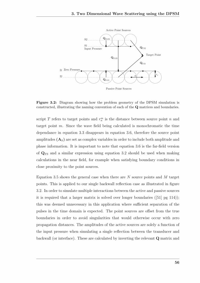
3. Two Dimensional Wave Scattering using the DPSM
QI1S2
QS1S2
QI1I2
S1
S2
I1
I2
Active Point Sources
Input Pressure
Passive Point Sources
Target Point
Zero Pressure
QTS2
QTI2
a rs
Figure 3.2: Diagram showing how the problem geometry of the DPSM simulation isconstructed, illustrating the naming convention of each of the Q matrices and boundaries.
script T refers to target points and rmn is the distance between source point n and
target point m. Since the wave field being calculated is monochromatic the time
dependance in equation 3.3 disappears in equation 3.6, therefore the source point
amplitudes (AS) are set as complex variables in order to include both amplitude and
phase information. It is important to note that equation 3.6 is the far-field version
of QTS and a similar expression using equation 3.2 should be used when making
calculations in the near field, for example when satisfying boundary conditions in
close proximity to the point sources.
Equation 3.5 shows the general case when there are N source points and M target
points. This is applied to our single backwall reflection case as illustrated in figure
3.2. In order to simulate multiple interactions between the active and passive sources
it is required that a larger matrix is solved over longer boundaries ([51] pg 114));
this was deemed unnecessary in this application where sufficient separation of the
pulses in the time domain is expected. The point sources are offset from the true
boundaries in order to avoid singularities that would otherwise occur with zero
propagation distances. The amplitudes of the active sources are solely a function of
the input pressure when simulating a single reflection between the transducer and
backwall (or interface). These are calculated by inverting the relevant Q matrix and
56

3. Two Dimensional Wave Scattering using the DPSM
multiplying by the input pressure boundary condition.
AS2 = [QS1S2]−1
ΨS1 (3.7)
At the interface, the pressure field created by the passive sources should be equal
to the field created by the active sources multiplied by the appropriate reflection
coefficients, as given by equation 3.8.
R =ρ2c2 cos θ1 − ρ1c1 cos θ2ρ2c2 cos θ1 + ρ1c1 cos θ2
(3.8)
where θ1 is the incident angle and θ2 is the transmitted angle measured from the
normal to the surface and c refers to the wavespeed in the respective media. If the
acoustic impedances of the two media are very different (as is the case with SH waves
within steel bounded by air) it can be assumed constant over the entire interface at
any angle of incidence and can be set equal to -1. During multiple scattering some
components of the transmitted field will interact with the surface at incident angles
differing from those predicted by the incident wave field alone. A constant reflection
coefficient makes the calculation of these extra components trivial; however, when
acoustic impedances are more similar this assumption cannot be made. Therefore
wherever multiple interactions occur, the reflection coefficient should be recalculated
for the solution to remain valid. This would substantially increase the complexity of
the simulation. Under such conditions the current simulation would therefore only
be valid when low levels of multiple scattering are expected. At the interface
QI1I2AI2 = QRI1S2AS2 (3.9)
therefore
AI2 = −1 ([QI1I2]−1
QI1S2AS2) (3.10)
where superscript R denotes multiplication by the reflection coefficient and Q matrix
subscripts should be inferred from Fig 3.2. Equation 3.10 represents the main advan-
tage over other rough surface scattering methods; multiple scattering and shadowing
effects are included in a single matrix inversion and multiplication process making
it very efficient and simple to implement. The incident field from the transducer
face and reflected field from the interface can now be calculated at any set of target
57
3. Two Dimensional Wave Scattering using the DPSM
points, hence the total field can be calculated.
ΨT = QTS2AS2 +QTI2AI2 (3.11)
Although Fig 3.2 illustrates the point sources separation (a) as double the offset from
the boundary (rs), the two distances can be set independently. Earlier publications
on DPSM have concluded that the upper limit of a should be set at one third of
the wavelength and that rs = a/√
2π in order to equate the effective hemispherical
area of the point sources to the area they occupy on the surface ([56], [51] pg 30).
It was found that in two dimensions the value of rs had little effect on the outcome
within certain bounds, determined by the accuracy of the Hankel function over short
distances and the minimum radius of curvature of the surface. To ensure each surface
was sampled sufficiently to reconstruct their true shape a point source separation of
50µm (a = λ/32) was selected. An offset to the boundary of 1.6µm (rs = λ/1000) was
chosen to prevent point source overlap across boundaries which have a low radius
of curvature. More rigorous studies into the effects of point source location at the
boundaries can be found in [65] and in Chapter 1 of [51].
3.2.3 Extension to the Time Domain
Pulses are used when calculating wall thickness so that the TOF can be determined.
To extend the monochromatic DPSM formulation to simulate time domain pulse
propagation, first the Fourier transform of the incident pulse f (t) at boundary S1
is determined.
F (ω) =1
√2π∫
∞
−∞f (t) exp (iωt)dt (3.12)
where F (ω) represents the frequency domain of the incident pulse. The calculations
detailed in the previous section are then carried out at each frequency component
within the Fourier transform, ensuring the pressure amplitude and phase from F (ω)
are defined in the vector ΨS1 in equation 3.7. Once the frequency domain signal
is constructed at target point m an inverse Fourier transform is used to transform
back to the time domain.
ψm (t) =1
√2π∫
∞
−∞Fm (ω) exp (−iωt)dω (3.13)
58

3. Two Dimensional Wave Scattering using the DPSM
In practice equations 3.12 and 3.13 are replaced with discrete sums and the fast
Fourier transform (FFT) and inverse fast Fourier transform (IFFT) are used. Mat-
lab [55] was chosen for writing the simulation since it is well suited to matrix ma-
nipulation and it allows the use of complex number matrices which are not always
supported in other programming environments. Separating the real imaginary com-
ponents would allow it to run on such platforms (see for example [66]); however, this
would increase the size and complexity of the matrices. The existing FFT, IFFT
and Hankel functions in Matlab were also found to perform rapidly and accurately
enough for our purposes. An alternative approach to using the DPSM to create
time dependent signals has been suggested by Rahani and Kundu [67] where the
Green’s function is used in the time domain, avoiding the need for Fourier analysis.
This approach, termed transient DPSM (t-DPSM), was discounted for the current
analysis as it is suited to situations where only a short section of the time domain
signal is required.
3.3 Comparison with the Kirchhoff Approxima-
tion
Once the DPSM simulation had been completed it was decided that it should be
compared with the most common simulation method found in rough surface scatter-
ing literature in order to highlight the benefits of the new technique. Approximate
analytical solutions making use of the Kirchhoff approximation were found to be the
most frequent, however many different forms of Kirchhoff theory exist, differing by
incident wave field type, defect boundary conditions, defect types and some which
attempt to include shadowing and higher order scattering. For the purpose of this
thesis, comparison will be made to classical scalar wave Kirchhoff theory which is
the most commonly implemented method used to investigate scalar wave reflection
from rough surfaces within literature. Equation 3.14 shows the final result given
by Schmerr [68] which calculates the scattered field at an observation point at a
distance r away from the crack face given the angle of incidence of the plane wave.
ψsct(r, k) = ψ0A(einc;esct)exp(ikr)
r(3.14)
59

3. Two Dimensional Wave Scattering using the DPSM
where k is the wavenumber of the incident wave, ψ0 is the incident amplitude,
einc is the unit normal along the incidence direction, esct is the unit normal along
the observation direction from the origin and A(einc;esct) is the far-field scattered
amplitude given by
A(einc;esct) = −ik
2π ∫S(einc ⋅ n) exp[ik(einc − esct) ⋅ xS)]dS (3.15)
In deriving equations 3.14 and 3.15 the following assumptions were made:
� Reflection is from a cracklike flaw with zero pressure on the lower surface and
a reflection coefficient of -1 on the upper surface.
� The crack is assumed to vary in height in one dimension only, resembling
ridges perpendicular to the scattering plane rather than hills which would be
expected in reality.
� The incident wave field is made up of monochromatic plane waves approaching
along unit vector ei.
� Amplitude A(einc;esct) is calculated in the far-field (r≫ λ)
� Scattering of waves between multiple parts of the crack is neglected.
� No shadowing of any part of the crack by any other part occurs when viewed
along einc or esct.
� Signals diffracted from crack tips are neglected.
Details on the mathematical derivation of equations 3.14 and 3.15 can be found in
[68].
3.3.1 Monochromatic Plane Wave Scattering
The simplifying assumption that the scattered amplitude is required only to be
calculated within the far-field (often referred to as the Fraunhofer approximation)
is commonly used during the derivation of approximate analytical scattering models
such as Kirchhoff theory. When considering the case of an ultrasonic transducer,
60
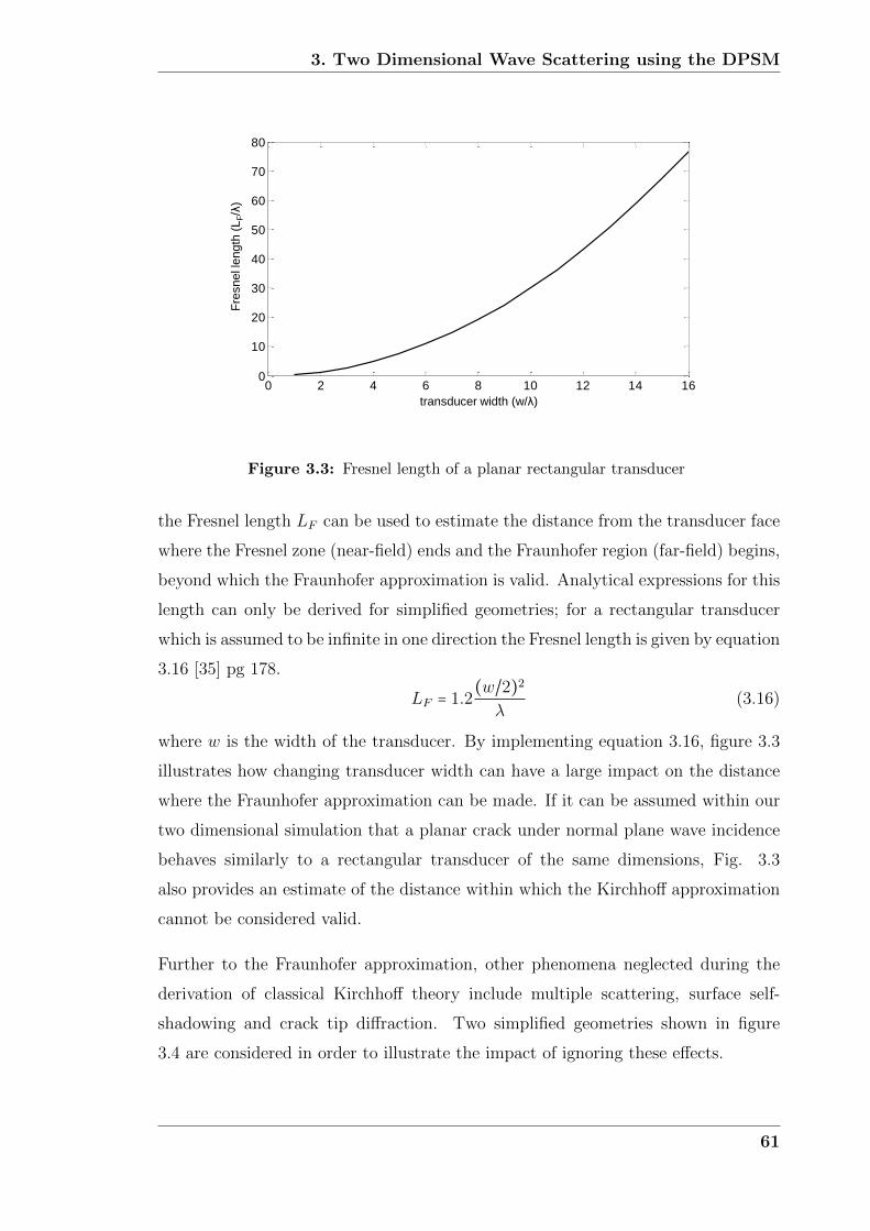
3. Two Dimensional Wave Scattering using the DPSM
0 2 4 6 8 10 12 14 160
10
20
30
40
50
60
70
80
crack length (Lc/)
fre
sn
el le
ng
th (
LF/
)
transducer width (w/λ)
Fre
sn
el le
ng
th (
LF/λ
)
Figure 3.3: Fresnel length of a planar rectangular transducer
the Fresnel length LF can be used to estimate the distance from the transducer face
where the Fresnel zone (near-field) ends and the Fraunhofer region (far-field) begins,
beyond which the Fraunhofer approximation is valid. Analytical expressions for this
length can only be derived for simplified geometries; for a rectangular transducer
which is assumed to be infinite in one direction the Fresnel length is given by equation
3.16 [35] pg 178.
LF = 1.2(w/2)2
λ(3.16)
where w is the width of the transducer. By implementing equation 3.16, figure 3.3
illustrates how changing transducer width can have a large impact on the distance
where the Fraunhofer approximation can be made. If it can be assumed within our
two dimensional simulation that a planar crack under normal plane wave incidence
behaves similarly to a rectangular transducer of the same dimensions, Fig. 3.3
also provides an estimate of the distance within which the Kirchhoff approximation
cannot be considered valid.
Further to the Fraunhofer approximation, other phenomena neglected during the
derivation of classical Kirchhoff theory include multiple scattering, surface self-
shadowing and crack tip diffraction. Two simplified geometries shown in figure
3.4 are considered in order to illustrate the impact of ignoring these effects.
61

3. Two Dimensional Wave Scattering using the DPSM
DPSM
Kirchhoff
DPSM
(a) (b)
Figure 3.4: Simplified crack geometries (a) 90○ angular crack used to demonstrate multi-ple scattering and surface self shadowing (b) 90○ incidence on planar crack used to comparediffracted signal amplitudes.
(a) (b)
0.2
0.4
0.6
0.8
1
30
210
60
240
90
270
120
300
150
330
180 0
DPSM
Kirchhoff
0.05
0.1
0.15
0.2
0.25
30
210
60
240
90
270
120
300
150
330
180 0
DPSM
Kirchhoff
Figure 3.5: Scattered amplitude under normal plane wave incidence (a) 90○ concaveangled crack (b) 90○ incidence on planar crack .
In all cases the simulated response is normalized to the maximum amplitude of the
centre frequency of the pulse when incident upon a flat defect of the same length and
at the same observation distance. Figure 3.5 shows the far-field scattered absolute
amplitude from the defects shown in Fig. 3.4. In the case of the concave angled crack
62

3. Two Dimensional Wave Scattering using the DPSM
with an internal angle of 90○, it would be expected that when a plane wave is incident
such that it approaches the faces of the crack at 45○ that almost all energy would
be directed back in the incident direction due to double scattering. The remaining
energy would contribute to diffracted waves at the crack tips. This response is clearly
demonstrated when using the DPSM simulation shown in Fig. 3.5(a). The Kirchhoff
approximation simulation instead shows two lobes perpendicular to the incidence
angle, each being half the amplitude of the incident wave. This response illustrates
not only that single scattering alone is calculated, it shows that components which
are scattered are free to subsequently travel through the crack face. This disregard
of self-shadowing is also shown in Fig. 3.5(b) where a lobe within the scattered field
downstream of the crack would be expected as indicated by the DPSM in order for
a shadow region to exist within the total field. Differences at all angles of incidence
in this case also indicate the lack of tip diffracted signals within the scattered field
predicted when using the Kirchhoff approximation.
Many authors have published investigations into the validity of the Kirchhoff ap-
proximation when modelling wave scattering from rough cracks with Gaussian dis-
tributed height and length characteristics; however most only consider the scattered
amplitude of monochromatic waves. Our specific application requires knowledge of
how the shape of an ultrasonic pulse which has reflected from a rough crack will
change, requiring both amplitude and phase to be accurately known. This approach
differs from the vast majority of literature on the subject, some examples of which
are provided as reference. While investigating acoustic wave scattering, Thorsos
[47] provides a thorough investigation into the surface variables which impact on
the validity of the Kirchhoff approximation, finding that surface correlation length
has a larger effect than the previously assumed RMS radius of curvature. Wombell
[69] reports how the Kirchhoff approximation is increasingly violated as RMS height
increases, showing rapid deterioration when σ/λ ≥ 0.2 while using it to reconstruct
rough surface profiles from scattered electromagnetic field data. When consider-
ing longitudinal ultrasonic wave scattering from rough cracks, Zhang et al [48] also
provide estimates of RMS height, correlation length and scattered angle values be-
yond which the Kirchhoff approximation can no longer be assumed valid. However,
providing definitive limits on the validity criteria of the Kirchhoff approximation
and other approximate scattering techniques through rigorous simulation of many
63

3. Two Dimensional Wave Scattering using the DPSM
rough surfaces historically has proven very difficult [39]. Therefore a detailed in-
vestigation was deemed outside the scope of this thesis and the interested reader
is referred to [37] [46] and [53] pg 100 for further information. For the Kirchhoff
approximation validity investigations carried out in this thesis a different approach
must be taken since it is incident pulse scattering which is of interest. Therefore
all subsequent analysis will be carried out by comparing signals in the time domain
using the theory in section 3.2.3 to convert monochromatic results.
3.3.2 Time Domain Plane Wave Pulse Scattering
In order to demonstrate how the tip diffracted waves can affect the simulated re-
sponse of a pulse reflecting from a crack of finite length, the diffracted components
must be separated from the main pulse. This can be achieved temporally using
equation 3.17 which calculates the crack length Lc required to completely separate
the diffracted pulses originating from the crack tips from the pulse reflecting from
the crack face.
Lc = 2√
2Lpr +L2p (3.17)
Where Lp is the required geometrical distance between the diffracted wave and main
pulse along the normal to the crack and r is the observation distance. A planar crack
under normal incidence is considered in order to simplify pulse shape and to ensure
diffraction is uniform at both tips. Clearly the difference in propagation distance
between the center of the crack and the tip tends to zero as observation distance
tends to infinity; therefore the simulation must be carried out within the Fresnel
zone in order to separate signals in this manner.
Using an observation distance of 5λ and a 2MHz 5 cycle pulse, a crack length of
17λ results in order to completely separate the main pulse from the tip diffracted
signals. Figure 3.6(a) shows the scattered response from such a defect, illustrating
how using the far field form of the equations inherent within the Kirchhoff approxi-
mation can affect the scattered response in the normal direction. In the same way
as monochromatic scattering, the simulated response is normalized to the maximum
amplitude of the centre frequency of the pulse when incident upon a flat defect of
the same length and at the same observation distance. Fig. 3.6(a) shows that the
64

3. Two Dimensional Wave Scattering using the DPSM
(a) (b)
2 4 6 8-1
-0.5
0
0.5
1
am
plit
ud
e (
arb
)
time (s)
DPSM
Kirchhoff
2 4 6 8-1
-0.5
0
0.5
1
am
plit
ud
e (
arb
)
time (s)
DPSM
Kirchhoff
Figure 3.6: Scattered signal at a distance of 5λ normal to the planar crack face undernormal incidence with a crack length of (a) 17λ (within near field) (b) 2λ (within far field).Thinner lines show the Hilbert envelopes of each signal.
phase is correctly predicted once diffracted components are removed; however, the
amplitude does not reduce by the amount consistent with a loss in energy due to
diffraction as is evident within the scattered signal produced by the DPSM simula-
tion. Figure 3.6(b) shows the same result when the observation is made in the far
field, obtained by changing the crack to be 2λ in length. It is clear that the diffracted
constituents are now incorporated within the main pulse, causing the energy con-
tent to be consistent between the two methods; however, the phase predicted by
the Kirchhoff approximation alters with respect to the DPSM simulation. Between
the near field and far field regions errors in the scattered response when using the
Kirchhoff approximation in the normal direction are a combination of amplitude
and phase, depending on diffracted signal location with respect to the main pulse.
Considering scattered angles other than the specular direction there are additional
errors associated when using the Kirchhoff approximation. Referring to equation
3.14, the position in time of the reflected pulse is calculated by changing the phase
of each constituent frequency by multiplying by exp(ikr)/r. This simply moves the
far field scattered response to the desired location in time without consideration of
near field effects. This has the greatest impact on error in directions other than
specular where near field contributions dominate as illustrated in figure 3.7 which
65

3. Two Dimensional Wave Scattering using the DPSM
time (s)
sca
tte
red
an
gle
()
2 4 6 8
-150
-100
-50
0
50
100
150
-1
-0.5
0
0.5
1
time (s)
sca
tte
red
an
gle
()
2 4 6 8
-150
-100
-50
0
50
100
150
0
10
20
30
40
50
time (s)
sca
tte
red
an
gle
()
22 24 26 28
-150
-100
-50
0
50
100
150
-1
-0.5
0
0.5
1
time (s)
sca
tte
red
an
gle
()
22 24 26 28
-150
-100
-50
0
50
100
150
0
10
20
30
40
50
time (s)
sca
tte
red
an
gle
()
22 24 26 28
-150
-100
-50
0
50
100
150
-1
-0.5
0
0.5
1
time (s)
sca
tte
red
an
gle
()
2 4 6 8
-150
-100
-50
0
50
100
150
-1
-0.5
0
0.5
1
am
plit
ud
e (
arb
)
am
plit
ud
e (
arb
)
en
ve
lop
e a
bso
lute
err
or
(%)
(a) (b) (c)
am
plit
ud
e (
arb
)
am
plit
ud
e (
arb
)
en
ve
lop
e a
bso
lute
err
or
(%)
(d) (e) (f)
Near
Fie
ld
Far
Fie
ld
DPSM Kirchhoff Difference
Figure 3.7: Time domain signals for all scattered angles around a planar crack with alength of 10λ. (a) Results from DPSM simulation with r = 7λ. (b) Results using Kirchhoffapproximation with r = 7λ. (c) Percentage difference in amplitude of the Hilbert enveloperesults from (a) and (b). (d) Results from DPSM simulation with r = 45λ (e) Resultsusing Kirchhoff approximation with r = 45λ (f) Percentage difference in amplitude of theHilbert envelope results from (d) and (e).
shows the scattered pulse recorded at all angles around the crack using the DPSM
and Kirchhoff approximation methods. Fig. 3.7(c) compares the amplitude pre-
dictions of the two methods by taking the difference of the Hilbert envelopes of
their scattered pulses when the planar crack is 10λ in length and the observation
distance is 7λ (LF /4). The envelopes were calculated to remove any errors caused
by slight variations in phase. Errors larger than 50% occur within 45○ either side of
the specular reflection, indicating the large impact the far field assumption has on
accuracy. Fig. 3.7(f) shows the same results but taken at an observation distance
of 45λ (3LF /2), illustrating the improvement in agreement within the Fraunhofer
region.
Using the far field assumption when considering a rough crack can have an even
66

3. Two Dimensional Wave Scattering using the DPSM
Near
Fie
ld
Far
Fie
ld
DPSM Kirchhoff Difference
time (s)
sca
tte
red
an
gle
()
2 4 6 8
-150
-100
-50
0
50
100
150
-0.5
0
0.5
am
plit
ud
e (
arb
)
en
ve
lop
e a
bso
lute
err
or
(%)
(a) (b) (c)
am
plit
ud
e (
arb
)
am
plit
ud
e (
arb
)
en
ve
lop
e a
bso
lute
err
or
(%)
(d) (e) (f)
am
plit
ud
e (
arb
)
time (s)
sca
tte
red
an
gle
()
22 24 26 28
-150
-100
-50
0
50
100
150
-0.5
0
0.5
time (s)
sca
tte
red
an
gle
()
22 24 26 28
-150
-100
-50
0
50
100
150
0
10
20
30
40
50
time (s)
sca
tte
red
an
gle
()
22 24 26 28
-150
-100
-50
0
50
100
150
-0.5
0
0.5
time (s)
sca
tte
red
an
gle
()
2 4 6 8
-150
-100
-50
0
50
100
150
-0.5
0
0.5
time (s)
sca
tte
red
an
gle
()
2 4 6 8
-150
-100
-50
0
50
100
150
0
10
20
30
40
50
Figure 3.8: Time domain signals for all scattered angles around a rough crack with alength of 10λ, an RMS height of λ/10 and a correlation length of λ/2. (a) Results fromDPSM simulation with r = 7λ (b) Results using Kirchhoff approximation with r = 7λ (c)Percentage difference in amplitude of the Hilbert envelope results from (a) and (b). (d)Results from DPSM simulation with r = 45λ (e) Results using Kirchhoff approximationwith r = 45λ (f) Percentage difference in amplitude of the Hilbert envelope results from(d) and (e).
larger impact on pulse shape prediction capability depending on scattered angle and
the shape of the particular rough crack. Figure 3.8 shows the scattered pulse shapes
at all observation angles around a rough crack with a length of 10λ, an RMS height
of λ/10 and a correlation length of λ/2. It is clear that when the observation distance
is just 7λ, the Kirchhoff approximation is unable to accurately predict pulse shape
with amplitude errors generally above 50% at all scattered angles between -90○ and
90○, including in the specular direction. However, when calculations are carried out
at an observation distance of 45λ, the Kirchhoff approximation is generally within
10% of the amplitude predicted by the DPSM as shown in Fig. 3.8(f). Errors
in this case will be caused by other factors such as neglecting multiple scattering,
self shadowing at high angles of incidence and tip diffraction which are dependent
67

3. Two Dimensional Wave Scattering using the DPSM
on roughness level and are outside the scope of this investigation. By inspecting
Fig. 3.3 which gives an estimate of where the Fraunhofer region begins, it is clear
that the relationship between crack length and the Fresnel length will be the main
limitation on the defect geometries where classical Kirchhoff theory can be applied.
The specific case of backwall reflection being investigated in this thesis will now be
considered.
3.3.3 Sensor Considerations
The reflection from an infinite backwall can be calculated up to a specified point in
time by modelling it as a long crack where the tip diffracted waves occur directly
after the total time to be simulated in the time domain signal. The length of this
crack can be calculated for a pulse echo inspection when considering only a single
backwall reflection from a cylindrical point source in 2D as shown by equation 3.18.
Lc = 2
√
(cttot
2)2
− T 2 (3.18)
Where T is the wall thickness and ttot is the total time to be simulated. Although
the sensor is not strictly pulse echo, equation 3.18 can be used as long as the pitch
between the transducers is much smaller than the wall thickness. Therefore, if the
wall thickness is 15mm and a simulated time of 15µs is required, a crack length
over 39mm results in order to make the simulated result equivalent to that from
an infinite backwall. Estimating the Fresnel length using equation 3.16, for a crack
length of 39mm a distance greater than approximately 280mm from the crack face
would be required to be within the Fraunhofer region of the scattered response and
for classical Kirchhoff theory to remain valid. In reality inspection is carried out
by the sensor at the upper surface of the wall, well within the Fresnel zone of the
backwall making the classical Kirchhoff theory approach unsuitable.
Many corrections have been proposed to improve the accuracy of Kirchhoff theory
in specific situations. Melton and Horton [70] investigate the use of the Fresnel cor-
rection, further highlighting the importance of accounting for different propagation
distances between points on a rough surface and the receiving transducer when cal-
culating phase and amplitude variations within the Fresnel zone. Bruce and Dainty
68

3. Two Dimensional Wave Scattering using the DPSM
[71] add an extra term which calculates any rays which have double scattered around
features on a rough interface, showing the increase in backscattered amplitude which
would be expected on surfaces with large RMS slope. They also include shadowing
in the same way as many other authors following the approach taken by Beckmann
[72] during early work using shadowing functions which have a value of 1 if the point
xS is illuminated by the incident wave and zero otherwise based on geometrical line
of sight. Bistatic shadowing is also included which accounts for shadowing from xS
to the receiver [38, 73]. However, all of these correction factors add to the complexity
of the Kirchhoff simulation that would have to be implemented in order to match
the accuracy provided by the DPSM.
One further important consideration is that the sensor does not transmit plane
waves. For analytical Kirchhoff theory to remain tractable the only alternatives read-
ily available within literature are plane wave beams with finite width and spherical
wave fields from point sources. One such example proposed by Berry [74] calculates
the pulse scattered from a rough surface by adding contributions from points on the
surface at specified geometrical distances away from the transceiver point source
to the corresponding location in the time domain signal. Being the closest exam-
ple found within literature to the situation of interest, it was subsequently applied
to the scattering of pulses from sinusoidal surfaces in my paper [31] showing good
agreement at low surface RMS heights. Multiple scattering effects do however cause
it to breakdown as RMS height increases, exhibiting little discernable improvement
in required simulation time when compared with the DPSM. Therefore, based on
the rapid simulation time achieved without any need for correction and its ease when
handling arbitrary incident fields, the DPSM was deemed superior to the Kirchhoff
approximation for the situations under investigation within this thesis and Kirchhoff
theory was not pursued any further.
3.4 Simulation Validation
In order to validate the DPSM simulation for use on more complex geometry, the
comparatively simple scenario of pulse scattering from a periodic sinusoidal surface
whose height varied in the x direction only was investigated. The equation for such
69

3. Two Dimensional Wave Scattering using the DPSM
z-axis (mm)
x-a
xis
(m
m)
-10 0 10
-15
-10
-5
0
5
10
15
0
0.2
0.4
0.6
(a) (b)
ma
ch
ine
d s
urf
ace
de
pth
(m
m)
Figure 3.9: (a) Schematic of experimental setup. (b) Plan view of the final stage ofthe machined sinusoidal surface. Areas within the dashed lines indicate the approximatelocations of the contact patches of each waveguide.
a surface is given by equation 3.19
h (x) =√
2σ cos(2πx
λs) (3.19)
where σ is the RMS height of the sinusoid and λs is the wavelength of the surface.
The RMS height was increased in stages to investigate how pulse shape changes when
compared with a flat surface. The FEM was chosen as the benchmark to compare
results to as it is an established numerical method capable of including all scattering
interactions along a boundary. Comparison was also made to experimental signals
obtained using the waveguide transducers in order to investigate whether the scalar
wave assumption can in fact be made when simulating SH wave scattering in two
dimensions.
The experimental setup, as illustrated in figure 3.9(a), was designed to investigate
the positional sensitivity a sensor made up of two waveguide transducers would
have when incident upon a given surface. This was achieved by adding a third
waveguide, therefore producing an array which replicated the situation where a single
sensor is moved between two positions separated by the pitch of the waveguides.
Physically moving the sensor during the experiment was not an option since slight
70
3. Two Dimensional Wave Scattering using the DPSM
changes in waveguide coupling would have a large impact on the received waveforms
which subsequently could not be compared with any accuracy. The waveguides were
assigned numbers from 1 to 3 as illustrated in Fig. 3.9(a), with signal sjl referring
to the waveform recorded by waveguide j when a pulse is transmitted by waveguide
l. The paths taken by signals s12 and s32 are shown in Fig. 3.9(a). The 2mm
pitch between the waveguides dictated the surface wavelength to be 4mm so that
one pair of waveguides would be incident directly above a trough in the surface
and the other pair incident above a peak. To mimic a two dimensional scattering
situation experimentally the profile shown in Fig. 3.9(b) was machined in 20µm
depth increments into the backwall of the 9.88mm thick mild steel test plate up to
a maximum RMS height of 0.28mm, beyond which the radius of curvature of the
ball nose cutter would cause errors in the machined surface. A full matrix capture
(FMC) data set was acquired after each machining stage using a TiePieSCOPE
HS805 which performed the roles of function generator and digital data acquisition
unit controlled using Matlab. The two dimensional plane modelled during simulation
was taken as the xy plane (z = 0) in Fig. 3.9(b), around which the beam profile in
the waveguide width direction is assumed symmetrical.
The FEM simulation, written using Abaqus explicit [75], was constructed using
the same backwall geometry and zero pressure boundary condition as the DPSM
simulation. Four node linear 2D acoustic quadrilateral elements were used with a
nominal node separation of 50µm and a simulation time step of 5ns which was stable
up to an RMS height of 0.26mm, beyond which increased mesh deformation required
smaller time steps. It was found that the built in non-reflecting acoustic boundary
conditions within Abaqus did not sufficiently damp out edge reflections; therefore
the problem domain was expanded to the minimum size required for no reflections to
encroach up to a total signal time of 10µs, resulting in a problem geometry containing
approximately 360000 elements. When run on a machine which had 256GB random
access memory and 4 quad-core 2.7GHz processors (AMD Opteron, Sunnyvale, CA)
a simulation time of 130 seconds was achieved. On the same machine the equivalent
DPSM simulation using the same point source separation as the node separation
(see section 3.2.2) took just 3 seconds, two orders of magnitude more rapid than the
FEM highlighting the efficiency of the technique.
71

3. Two Dimensional Wave Scattering using the DPSM
Sim
ula
ted
sig
nals
(s
12)
Sim
ula
ted
sig
nals
(s
32)
6 8 10-0.2
-0.1
0
0.1
0.2
time (s)
am
plit
ud
e (
arb
)
RMS height = 0.1mm
DPSM
FEM
6 8 10-0.2
-0.1
0
0.1
0.2
time (s)
am
plit
ud
e (
arb
)
RMS height = 0.2mm
DPSM
FEM
6 8 10-0.2
-0.1
0
0.1
0.2
time (s)
am
plit
ud
e (
arb
)
RMS height = 0.3mm
DPSM
FEM
6 8 10-0.2
-0.1
0
0.1
0.2
time (s)
am
plit
ud
e (
arb
)
RMS height = 0.1mm
DPSM
FEM
(a) (b)
(d)
(c)
(e) (f)
6 8 10-0.2
-0.1
0
0.1
0.2
time (s)
am
plit
ud
e (
arb
)
RMS height = 0.2mm
DPSM
FEM
6 8 10-0.2
-0.1
0
0.1
0.2
time (s)
am
plit
ud
e (
arb
)
RMS height = 0.3mm
DPSM
FEM
(Pa
) (P
a)
Figure 3.10: Simulated signals s12 obtained using the DPSM and FEM simulations withan input pressure amplitude of 1, showing the unscaled reflected scalar wave pulse froma sinusoidal surface with RMS heights of (a) 0.1mm, (b) 0.2mm and (c) 0.3mm. Similarresults for signals s32 and RMS heights of (d) 0.1mm, (e) 0.2mm and (f) 0.3mm. Dottedlines show the Hilbert envelopes of each signal.
Simulated signals from both pairs of waveguides within the array are shown in figure
3.10 which have not been scaled from the raw outputs produced by the FEM or the
DPSM simulations based on an input pressure amplitude of 1Pa at the transmitting
waveguide. To calculate the final signal an average of all the signals calculated at
the nodes / target points within the 0.5mm long receiver contact patch was taken.
The results from the DPSM are almost indistinguishable from the FEM, illustrating
no need for amplitude scaling as is reported for the DPSM in three dimensional
scattering problems [76]. This is most likely because ignoring contributions between
point sources at the surface has a much reduced effect in two dimensions because
of the large reduction in effective area being ignored. Using denser point sources
distributions along a boundary produces the same simulated result. Based on such
strong agreement and much improved efficiency, the DPSM was used to carry out
all future two dimensional scalar wave simulated results presented within this thesis.
72

3. Two Dimensional Wave Scattering using the DPSM
Exp
eri
men
tal
Sim
ula
ted
6 8 10
-1.5
-1
-0.5
0
0.5
1
1.5
RMS height = 0.12mm
time (s)
am
plit
ud
e (
arb
)
sref
s12
s32
6 8 10
-1.5
-1
-0.5
0
0.5
1
1.5
RMS height = 0.28mm
time (s)
am
plit
ud
e (
arb
)
sref
s12
s32
6 8 10
-1.5
-1
-0.5
0
0.5
1
1.5
RMS height = 0.2mm
time (s)
am
plit
ud
e (
arb
)
sref
s12
s32
202 204 206
-1.5
-1
-0.5
0
0.5
1
1.5
time (s)
am
plit
ud
e (
arb
)
RMS height = 0.28mm
sref
s12
s32
202 204 206
-1.5
-1
-0.5
0
0.5
1
1.5
time (s)
am
plit
ud
e (
arb
)
RMS height = 0.2mm
sref
s12
s32
202 204 206
-1.5
-1
-0.5
0
0.5
1
1.5
time (s)
am
plit
ud
e (
arb
)
RMS height = 0.12mm
sref
s12
s32
(a) (b)
(d)
(c)
(e) (f)
Figure 3.11: Experimental signals showing the reflected SH wave pulse from a onedimensional sinusoidal surface with a surface wavelength of 4mm and RMS heights of(a) 0.12mm, (b) 0.20mm and (c) 0.28mm. Simulated signals obtained using the twodimensional scalar wave DPSM model from the same surface with RMS heights of (d)0.12mm, (e) 0.20mm and (f) 0.28mm. Dotted lines show the Hilbert envelopes of eachsignal.
Experimental signals from both waveguide pairs at RMS heights of 0.12, 0.2 and
0.28mm are shown in figure 3.11 alongside equivalent signals calculated using the
DPSM simulation. In each case the signals were normalized to a reference signal sref ,
taken as the reflected pulse when the backwall was flat which is also shown in Fig.
3.11 for amplitude and phase comparison. Additionally, it was found that because of
the comparatively long length of the waveguides that ambient temperature changes
occurring during the course of the experiment caused the arrival times of the surface
skimming wave which travels directly from transmitter to receiver to change by up
to 0.1µs. In order to isolate changes in pulse shape caused by backwall shape change
from those caused by external environmental factors, the temperature compensation
strategy presented by Croxford et al [77] was implemented using the surface skim-
ming waves as reference signals since in theory they should not be affected during
machining.
73

3. Two Dimensional Wave Scattering using the DPSM
It is clear by comparing the shape of the Hilbert envelopes of the signals in Fig. 3.11
that the majority of physical interactions occurring during reflection at the backwall
are captured using the scalar wave approach. Taking s12 for example, the initial
increase in amplitude and subsequent split into two smaller amplitude peaks with
the later arriving peak constructively interfering to be higher in amplitude as RMS
height approaches 0.28mm is predicted well using the simulation. Similarly for s32
the simulation closely matches the experimental results showing the initial decrease
in amplitude and subsequent large increase in both pulse maximum amplitude and
tail length caused by energy being backscattered from areas on the surface further
from the receiver. By inspection the relative phase changes from sref to s12 and s32
also appear to match closely.
However differences are clearly evident which are thought to be primarily caused by
insufficient mode purity within the waveguide transducers. While experimentally
assessing SH0* mode purity within similar transducers by looking at the pulse echo
signals reflected from the end of the waveguide, Cegla reports that higher order
modes which are around 30dB weaker than the primary mode are observed [26].
These modes which are evident immediately following the surface skimming wave,
as illustrated in figure 3.12, have a larger impact when performing pitch catch in-
spection of a backwall, being on average only 22dB weaker than sref . Through
constructive and destructive interference it is expected that these modes will cause
amplitude errors, represented as error bars in figure 3.13 which illustrate the bounds
within which the envelope maximum amplitude is expected to lie as RMS height
increases. Experimental results for RMS heights lower than 0.12mm have been omit-
ted because it was clear by visual inspection of the machined surfaces that the CAM
software used by the milling machine failed to generate the required tool paths.
74

3. Two Dimensional Wave Scattering using the DPSM
1
2
194 196 198 200 202 204 206 208
-1
-0.5
0
0.5
1
time (s)
am
plit
ud
e (
arb
)
Unwanted wavemodes
1
2
(a) (b)
Figure 3.12: (a) Diagram of paths taken by the surface skimming wave and backwall re-flection from the transmitter to the receiver. (b) Experimental signal taken when backwallwas flat, illustrating the unwanted modes travelling along the waveguides adding coherentnoise which is on average 22dB lower than the amplitude of the backwall reflection.
0 0.05 0.1 0.15 0.2 0.25 0.3-12
-10
-8
-6
-4
-2
0
2
4
6
RMS height (mm)
ma
xim
um
en
ve
lop
e a
mp
litu
de
(d
B)
DPSM s32
DPSM s12
Experimental s32
Experimental s12
Figure 3.13: Comparison of the maximum envelope amplitude measured experimentallyand calculated using the two dimensional scalar wave DPSM simulation for both waveguidepairs within the 3 waveguide array. Error bars represent the -22dB amplitude error thatcould be introduced by unwanted modes travelling within the waveguides.
75

3. Two Dimensional Wave Scattering using the DPSM
The simulated amplitude trend for s32 shown in Fig. 3.13 is within 0.9dB of ex-
perimental results at all RMS heights; however, agreement is not so close for s12.
A 20% reduction in amplitude of the reference signal between waveguides 1 and 2
indicates that coupling quality, and therefore signal quality, is the most likely cause.
However, in both cases the amplitude trends and signal shape changes produced
using the DPSM simulation match experimental results closely, indicating that the
scalar wave approach is valid for predicting SH wave scattering in two dimensional
geometries. The large decrease in simulation complexity associated with making
the scalar wave assumption is particularly beneficial when studying the effects of
surface roughness where ensemble averaging must carried out, therefore making it
an important approximation within all subsequent work presented in this thesis.
3.5 Rough Surface Spatial Frequency Content
Before proceeding onto pulse scattering from rough surfaces, it is important to assess
the limits of roughness which will have an impact on the shape of the scattered pulse.
Many non-dimensional numbers have been suggested as a way of defining the level
of roughness, in particular for the purpose of advising when diffuse components
will dominate over coherent reflections. The most commonly used is the Rayleigh
criterion in conjunction with the Rayleigh parameter, derived by considering plane
waves scattering from sinusoidal surfaces. By summing contributions at a target
location within the scattered field from all points along a surface, it was proposed
that a rough surface could be considered smooth if:
kσcosθ <π
4(3.20)
where k is the wavenumber, θ is the incident and reflected angle and the value of the
left hand side of the equation is known as the Rayleigh parameter [53]. Otherwise
the surface should be considered rough and the diffuse field will dominate. For a
2MHz SH wave in steel under normal incidence this suggests that RMS heights above
0.2mm (λ/10) can be considered rough. As such RMS heights up to 0.3mm (∼ λ/5)
will be considered within this thesis to ensure that the majority of signal coherency
is lost. However, the Rayleigh parameter does not consider horizontal length scales
76

3. Two Dimensional Wave Scattering using the DPSM
x-axis (mm)
y-a
xis
(m
m)
-10 -5 0 5 10
10
8
6
4
2
0-2
-1
0
1
2
x-axis (mm)
y-a
xis
(m
m)
-10 -5 0 5 10
10
8
6
4
2
0-2
-1
0
1
2
x-axis (mm)
y-a
xis
(m
m)
-10 -5 0 5 10
10
8
6
4
2
0-2
-1
0
1
2
x-axis (mm)
y-a
xis
(m
m)
-10 -5 0 5 10
10
8
6
4
2
0-2
-1
0
1
2
(a) (b)
(c) (d)
am
plit
ud
e (
arb
) a
mp
litu
de
(a
rb)
Figure 3.14: Scattered field when a 2MHz plane wave with a velocity of 3260ms−1 isnormally incident upon a sinusoidal backwall with an RMS height of 0.1mm and a surfacewavelength (λs) of (a) 0.5mm, (b) 2mm, (c) 8mm and (d) 50mm.
which are more difficult to define in terms of a transition to surface roughness.
Factors such as the RMS slope and RMS curvature which incorporate horizontal
length measures have been used to define limits on the validity of the Kirchhoff
approximation [47, 54], mainly for reasons of multiple scattering; however, they give
no indication of the horizontal feature length limits outside which a surface should
be considered rough. The challenge faced in defining such a limit is illustrated in
figure 3.14, which shows the near field amplitude of the scattered wave field when a
normally incident plane wave reflects from sinusoidal surfaces with RMS heights of
0.1mm but with different surface wavelengths (λs).
When horizontal feature lengths are much smaller than the incident wavelength, as
can be seen in Fig. 3.14 (a), the ultrasound cannot interact with the small features
and reflection is identical to that which would be experienced if the surface was flat
along the peaks of the sinusoid. Conversely if the features are much larger than the
incident wavelength, as can be seen in Fig. 3.14 (d), the surface is essentially flat
from the point of view of the incident wave and reflection behaviour is very similar
to that of a flat backwall. In between these two limits however, the interference field
77

3. Two Dimensional Wave Scattering using the DPSM
0 5 10 15-40
-30
-20
-10
0
ave
rag
e a
mp
litu
de
(d
B)
horizontal length scale within rough surface (l/)
0=/4
0=/2
0=
0=3/2
Figure 3.15: Average Fourier transforms of 5000 rough surfaces with the same correla-tion lengths for various correlation length values, indicating the length scales of featurespresent within the surfaces. Amplitudes are relative to the length scale with the largestcontribution to the average spatial frequency content.
can have a very complex structure which is difficult to predict and dependent on
the surface wavelength.
When considering rough surfaces, the interference patterns become much more diffi-
cult to predict since the surface structure contains features of varying length scales.
This is illustrated in figure 3.15 where the spatial frequency content of rough sur-
faces described using Gaussian height and length characteristics has been analysed
by calculating the Fourier transform of 5000 rough surfaces generated using the same
correlation lengths and RMS heights and averaging their result. The relationship
illustrates that the correlation length parameter performs as expected, effectively
acting like a length-scale high pass filter, allowing features with longer lengths to
remain in the final rough surface during the moving average procedure described in
section 2.4. However, it also indicates that various length scales act concurrently
during ultrasonic wave reflection from rough surfaces to produce very complex scat-
tered fields. Therefore it can be concluded that RMS height is the dominant factor
in establishing whether a surface should be considered rough using equation 3.20,
and whether diffuse energy will dominate. Correlation length simply has to be of a
similar order of magnitude to the incident wavelength in order for diffuse energy to
exist within the scattered field. Within this thesis correlation length will be varied
from 0.4mm (λ/4) up to 2.4mm (3λ/2) to produce a wide range of surface shapes
78

3. Two Dimensional Wave Scattering using the DPSM
for analysis (see Fig. 2.3).
3.6 Summary
The DPSM has been presented as an alternative simulation method for use when
investigating how scalar waves interact with rough surfaces in two dimensions. Scat-
tering simulations using classical Kirchhoff theory were identified as the most com-
monly implemented within literature; therefore a comparison was carried out to
highlight the benefits of the new technique. It was found that although multiple
scattering, surface self-shadowing and tip diffraction all affect the accuracy of the
Kirchhoff approximation, it was the far-field assumption and the need for an ar-
bitrary incident field which most limited its applicability for the rough backwall
situation being investigated within this thesis. In all cases the DPSM showed im-
proved accuracy with little increase in required simulation time.
Comparison was also made to simulated results produced using the FEM in order
to validate the true accuracy of the technique. A sinusoidal backwall was chosen
rather than a rough backwall in order to produce repeatable results with potentially
high reflected pulse shape variability based on sensor position. Without any need
for scaling, the results produced by the DPSM were indistinguishable from those
produced using the FEM at RMS heights up to 0.3mm (∼ λ/5), providing confidence
in the accuracy of the technique. When carried out on the same machine the DPSM
calculated each simulated waveform within 3 seconds whereas the FEM took around
130 seconds, approximately two orders of magnitude slower. Based on its accuracy
and efficiency the DPSM simulation was the clear choice for carrying out future
roughness investigations in two dimensions.
Comparison with experimental results on the same sinusoidal surface was carried
out in order to verify that the scalar wave approximation was a valid approach
when simulating SH wave scattering in two dimensions. Good agreement in both
pulse shape and envelope maximum amplitude trends as RMS height increased was
achieved. Unwanted modes travelling within the waveguide transducers were found
to be the main source of error; however, the close agreement indicates that the scalar
79

3. Two Dimensional Wave Scattering using the DPSM
wave approximation is valid when simulating SH wave scattering in two dimensions
by periodic corrugated surfaces. Now that the technique has been experimentally
validated, the focus of the next chapter will its application to the practical problem
of wall thickness monitoring and what impact corrosion at the reflecting surface can
have on thickness estimate based on the ultrasonic data.
80
Chapter 4
Thickness Monitoring and Surface
Roughness Detection
4.1 Introduction
The previous chapter discussed how the DPSM simulation was developed for mod-
elling ultrasonic pulse reflection from rough surfaces. In this chapter it will be used
to investigate the uncertainty in measured wall thickness caused by diffuse energy
being introduced into the pulse by the rough surface. The altered shape of the
reflected pulse affects how accurately the time of flight (TOF) algorithm can dis-
tinguish when the pulse is received by the sensor, and therefore the wall thickness
estimate produced. This is demonstrated by the simulated results shown in figure
4.1 which shows the working principles of the ultrasonic waveguide sensor, as well as
the simulated signal when the inner surface is flat and an example when the inner
surface has an RMS height of 0.2mm (σ = λ/8) and a correlation length of 0.8mm
(λ0 = λ/2).
The sensor [30] operates by sending a pulse down one waveguide and receiving along
the other (pitch-catch mode) to overcome high coupling losses on transmission into
the component wall. If the distance to the inner surface is larger than the sep-
aration between the transmitter and receiver, the received signal will record two
distinct pulses; the first is the surface skimming wave directly between the trans-
81

4. Thickness Monitoring and Surface Roughness Detection
0 2 4 6 8 10-0.25
-0.2
-0.15
-0.1
-0.05
0
0.05
0.1
0.15
0.2
time (s)
am
plit
ud
e (
Pa
)
Flat
Roughsurface
skimming
wave
backwall
reflection
(a)
(b)
inner surface
transducer
HO
T
CO
LD
T
component wall
aw
tran
smit
tin
g w
aveg
uid
e
rece
ivin
g w
aveg
uid
e
outer surface
y
x
Figure 4.1: (a) Schematic of wall thickness sensor showing paths taken by surface skim-ming wave and backwall reflection. (b) Simulated signals from a flat backwall and arough backwall when σ = 0.2mm and λ0 = 0.8mm showing the surface skimming wave andbackwall reflection which would be received and used to calculate wall thickness.
mitter and receiver and the second is the reflection from the inner surface (ignoring
any material backscatter and multiple reflections between inner and outer surfaces
that arrive at later points in time). Once the TOF of the surface skimming wave
t1 and the backwall reflection t2 are determined, the estimated wall thickness T can
be calculated using equation 4.1
T =1
2
√[(t2 − t1)c + aw]2 − a2w (4.1)
Where aw is the separation between the transmitter and receiver and c is the
wavespeed which is linearly dependent on temperature and can be corrected for
using known material properties and temperature values [30, 78]. Simply through
observation of the rough surface signal in Fig. 4.1 (b) it is clear that any operator
or TOF algorithm would struggle to accurately determine the arrival time of the
reflected pulse; the value produced depending on what aspect of the signal is being
used to make the estimate. Three commonly implemented TOF algorithms will be
introduced and applied to simulated signals produced by the DPSM simulation and
in doing so will provide stability limits for each algorithm.
82

4. Thickness Monitoring and Surface Roughness Detection
Additional to determining the stability of each TOF algorithm under corrosive condi-
tions, it will also be investigated whether the shape change caused by diffuse energy
introduced by surface roughness can be used directly to evaluate the uncertainty
limits on the thickness estimate. This would increase both information content and
confidence in the final value provided. All results presented are for two dimensional
scattering from Gaussian distributed rough surfaces and as such should be treated
as a worst case scenario for the RMS height and correlation length values quoted.
It is expected that for a surface with similar surface statistics in three dimensions
that spatial averaging should reduce the extreme effects of roughness (see Chapter
5).
4.2 Scattered Pulse Shape Change Caused by Sur-
face Roughness
The majority of investigations into the effects of surface roughness found in literature
consider only monochromatic plane wave scattering, primarily focussing on signal
amplitude and reflection coefficient change with incident and reflection angle. In
isolation these results give no indication of the shape changes that can occur to
pulses in the time domain when reflecting from such surfaces. This severely limits
the applicability of such research when signal shape is of primary concern, such
as the situation being investigated within this thesis. Therefore, unlike the vast
majority of literature our approach focusses on reflected pulse shape change in the
time domain, making the results more relevant in practical TOF applications.
4.2.1 DPSM Simulation
A simulation that replicates the sensor setup was created: the separation between
the transmitter and receiver was 2mm with estimated 0.5mm contact lengths at the
locations where each waveguide couples to the test specimen. To create a single
signal at the receiver the reflected pulse is calculated at each target point along
the contact and an average signal is calculated. A point source separation of 50µm
was used (a = λ/32), similarly to section 3.2.2, resulting in 533 passive point sources
83
4. Thickness Monitoring and Surface Roughness Detection
making up the inner surface which were separated from the true boundary by 1.6µm
(rs = λ/1000). At each combination of RMS height (0.02 to 0.3mm in 0.02mm incre-
ments) and correlation length (0.4, 0.8, 1.6 and 2.4mm) 500 surfaces were generated
having the same mean wall thicknesses and the corresponding signals were simu-
lated. Similar results are shown in my paper [31] which used a mean wall thickness
of 15mm. To remain consistent with other results given in this thesis, simulations
were rerun using a mean wall thickness of 10mm showing little difference in terms
of scattered signal shapes and TOF algorithm stability. Therefore relevant excerpts
from [31] have been reproduced in sections 4.2.2 and 4.3.2, changing only some
numerical values quoted in the results.
4.2.2 Individual Signal Analysis
Figure 4.2 (a), (b) and (c) show the scattered pulses and surface profiles of three
realizations of surfaces with an RMS height of 0.2mm (σ = λ/8) and a correlation
length equal to the incident centre frequency wavelength (λ0 = λ). The flat backwall
response is shown as a blue line in each plot to serve as reference for the change in
pulse shape. It is clear that surfaces with similar statistics can produce scattered
pulses with very large fluctuations in amplitude. Figures 4.2(a) and (b) show the
signals with the highest and lowest amplitudes in the data set when σ = λ/8 and λ0 =
λ, caused by constructive and destructive interference at the receiver respectively.
The shapes of these signals are also quite distorted from the incident pulse; however,
Fig. 4.2(c) illustrates that a response can equally show little evidence of scattering
by a rough surface. This result indicates that the inverse scattering problem of
reconstructing a surface profile from its reflected response would be impossible from
a fixed position using a single thickness sensor.
If the correlation length is decreased, other effects can be observed in the signals as
illustrated in Fig. 4.2 (d), (e) and (f) which show three signals and corresponding
surfaces having the same RMS height (σ = λ/8) but a correlation length of half
the incident centre frequency wavelength (λ0 = λ/2). In this case more features
exist on the surface which are further away from the transmitter that act to reflect
energy back to the receiver, culminating in more pronounced tails on the signals as
illustrated in Fig 4.2(d). This leads to other effects such as pulse stretching and
84

4. Thickness Monitoring and Surface Roughness Detection
6 8 10-0.2
-0.1
0
0.1
0.2
time (s)
am
plit
ude (
Pa)
RMS height = 0.2mm
Flat
Rough
6 8 10-0.2
-0.1
0
0.1
0.2
time (s)
am
plit
ude (
Pa)
RMS height = 0.2mm
Flat
Rough
-10 0 10
-101
x (mm)
y (
mm
)
-10 0 10
-101
x (mm)
y (
mm
)
6 8 10-0.2
-0.1
0
0.1
0.2
time (s)
am
plit
ude (
Pa)
RMS height = 0.2mm
Flat
Rough
-10 0 10
-101
x (mm)
y (
mm
)
λ0 =
λ
(a.i) (b.i)
(d.i)
(c.i)
(e.i) (f.i)
λ0 =
λ/2
(a.ii) (b.ii)
(d.ii)
(c.ii)
(e.ii) (f.ii)
-10 0 10
-101
x (mm)
y (
mm
)
6 8 10-0.2
-0.1
0
0.1
0.2
time (s)
am
plit
ude (
Pa)
RMS height = 0.2mm
Flat
Rough
6 8 10-0.2
-0.1
0
0.1
0.2
time (s)
am
plit
ude (
Pa)
RMS height = 0.2mm
Flat
Rough
-10 0 10
-101
x (mm)
y (
mm
)
6 8 10-0.2
-0.1
0
0.1
0.2
time (s)am
plit
ude (
Pa)
RMS height = 0.2mm
Flat
Rough
-10 0 10
-101
x (mm)
y (
mm
)
Figure 4.2: Simulated scattered pulse shapes and surface profiles for three surfaces whereσ = λ/8 and λ0 = λ illustrating examples of (a) high ampltiude (b) low amplitude, and (c)similarity to flat backwall response. Simulated Signals with the same σ value but λ0 = λ/2showing examples of (d) energy in signal tail, (e) stretched/offset pulse, and (e) multiplepulses. Each signal is shown alongside the specific surface from which it reflected.
apparent increases in arrival time and overestimation of wall thickness (see Fig.
4.2(e)), the extent of which is dependent on the choice of TOF algorithm. Multiple
pulses can also be observed in many signals such as those in Fig 4.2(f), casting doubt
over final thickness values and phantom defect responses.
This short summary of potential signal shapes illustrated in Fig 4.2 is by no means
exhaustive or representative; the majority of signals contain varying levels of diffuse
energy creating an almost infinite number of possible scattered pulse shapes. The
general conclusions that can be drawn however are that RMS height has a much
greater impact on signal shape and amplitude than correlation length, imparting
greater levels of diffuse energy as it is increased. This is further illustrated in Fig
85

4. Thickness Monitoring and Surface Roughness Detection
0 0.02 0.04 0.06 0.08 0.1 0.12 0.14 0.16 0.180.08
0.085
0.09
0.095
0.1
0.105
RMS height (/)
me
dia
n m
axim
um
en
ve
lop
e a
mp
litu
de
(P
a)
0=/4
0=/2
0=
0=2/3
Figure 4.3: Comparison of the median maximum amplitude of Hilbert envelope of re-flected pulses from surfaces with RMS heights up to 0.3mm (σ < λ/5) and correlationlengths between 0.4mm and 2.4mm (λ/4 < λ0 < 2λ/3).
4.3 where the maximum amplitude from each reflected pulse is used as a measure
of pulse change due to surface roughness. Taking the median value of the distri-
bution at each RMS height decreases the impact of outliers and indicates the most
likely change in amplitude which could be expected. It can be observed that pulse
amplitude decreases as RMS height increases; this is caused by energy being prefer-
entially scattered away from the receiver as roughness normal to the incident wave
increases. However, changing correlation length is seen to have little effect on the
most probable amplitude change. The results given in Figs 4.2 and 4.3 clearly il-
lustrate the variability in scattered pulse shape a TOF algorithm might encounter
when monitoring the wall thickness of corroded components.
4.2.3 Ensemble Averaged Results
Ensemble averaging is carried out by calculating many signals from surfaces pos-
sessing the same σ and λ0 values and averaging their result. This produces the
coherent constituent of the reflected signal, signifying on average what the most
likely reflected response would be from such a surface. Subsequently subtracting
this coherent constituent from an individual scattered response provides the diffuse
86

4. Thickness Monitoring and Surface Roughness Detection
0 1 2 3 4 5 6 7 8 9 10-0.2
-0.15
-0.1
-0.05
0
0.05
0.1
0.15
0.2
time (s)
am
plit
ud
e (
Pa
)
flat backwall
rough backwall
coherent
diffuse
Figure 4.4: Example rough backwall simulated signal, showing the coherent componentcalculated using 500 simulated signals and the diffuse component.
component of the reflected signal. In general as roughness increases it is expected
that coherency should reduce, while diffuse components which scatter from many
points on the surface should increase depending on the position of the observer. A
comparison of these signal constituents for a time domain pulse is shown in figure
4.4 for a surface with an RMS height of 0.2mm (σ = λ/8) and a correlation length
of 0.8mm (λ0 = λ/2).
Many (if not all) authors who have published work investigating the effects of sur-
face roughness use ensemble averaging to damp out the large variations in amplitude
and phase that can occur, thereby producing clear conclusions on the most prob-
able trends that might be observed under given conditions. In a practical sense
these results cannot be utilised without the possibility of averaging over a given
surface, usually spatially by scanning a probe. In permanently installed monitoring
situations this is clearly impractical where signals are only available from a single
location. In this case a temporal average could be taken; however, the surfaces are
not independent through time, therefore features developing on the surface (assum-
ing gradual change) will affect the signals in a similar way, not allowing ensemble
averaging to take place. Accounting for this lack of applicability, ensemble aver-
aged results can give insight into expected changes to signals and therefore will be
examined briefly.
87
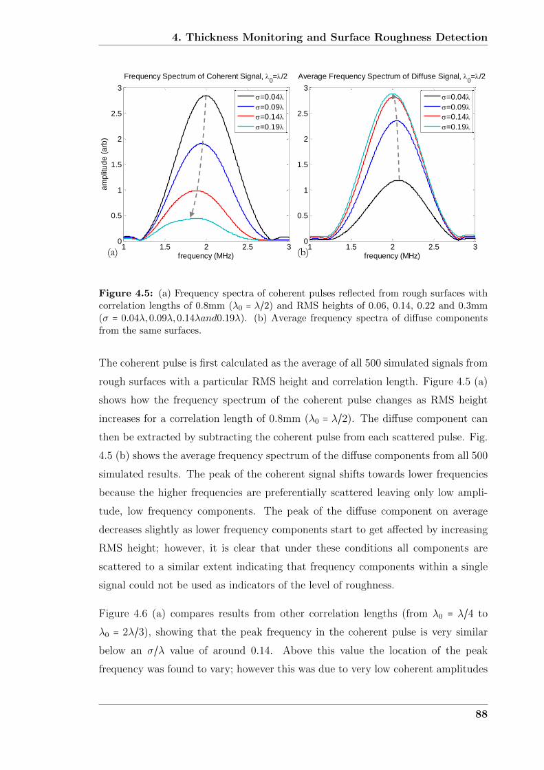
4. Thickness Monitoring and Surface Roughness Detection
1 1.5 2 2.5 30
0.5
1
1.5
2
2.5
3
frequency (MHz)
am
plit
ud
e (
arb
)
Average Frequency Spectrum of Diffuse Signal, 0=/2
=0.04
=0.09
=0.14
=0.19
1 1.5 2 2.5 30
0.5
1
1.5
2
2.5
3
frequency (MHz)
am
plit
ud
e (
arb
)
Frequency Spectrum of Coherent Signal, 0=/2
=0.04
=0.09
=0.14
=0.19
(a) (b)
Figure 4.5: (a) Frequency spectra of coherent pulses reflected from rough surfaces withcorrelation lengths of 0.8mm (λ0 = λ/2) and RMS heights of 0.06, 0.14, 0.22 and 0.3mm(σ = 0.04λ,0.09λ,0.14λand0.19λ). (b) Average frequency spectra of diffuse componentsfrom the same surfaces.
The coherent pulse is first calculated as the average of all 500 simulated signals from
rough surfaces with a particular RMS height and correlation length. Figure 4.5 (a)
shows how the frequency spectrum of the coherent pulse changes as RMS height
increases for a correlation length of 0.8mm (λ0 = λ/2). The diffuse component can
then be extracted by subtracting the coherent pulse from each scattered pulse. Fig.
4.5 (b) shows the average frequency spectrum of the diffuse components from all 500
simulated results. The peak of the coherent signal shifts towards lower frequencies
because the higher frequencies are preferentially scattered leaving only low ampli-
tude, low frequency components. The peak of the diffuse component on average
decreases slightly as lower frequency components start to get affected by increasing
RMS height; however, it is clear that under these conditions all components are
scattered to a similar extent indicating that frequency components within a single
signal could not be used as indicators of the level of roughness.
Figure 4.6 (a) compares results from other correlation lengths (from λ0 = λ/4 to
λ0 = 2λ/3), showing that the peak frequency in the coherent pulse is very similar
below an σ/λ value of around 0.14. Above this value the location of the peak
frequency was found to vary; however this was due to very low coherent amplitudes
88

4. Thickness Monitoring and Surface Roughness Detection
0 0.05 0.1 0.15 0.21.7
1.8
1.9
2
2.1
RMS height (/)
pe
ak fre
qu
en
cy (
MH
z)
Coherent, 0=/4
Diffuse, 0/4
Coherent, 0=/2
Diffuse, 0=/2
Coherent, 0=
Diffuse, 0=
Coherent, 0=2/3
Diffuse, 0=2/3
0 0.05 0.1 0.15 0.20
0.5
1
1.5
2
2.5
3
3.5
RMS height (/)
pe
ak a
mp
litu
de
(a
rb)
Coherent, 0=/4
Diffuse, 0/4
Coherent, 0=/2
Diffuse, 0=/2
Coherent, 0=
Diffuse, 0=
Coherent, 0=2/3
Diffuse, 0=2/3
(a)
(b)
Figure 4.6: (a) Peak frequencies in frequency spectra of coherent pulse and averagefrequency spectra of diffuse components for all RMS height values (0.02 to 0.3mm in0.02mm increments) and correlation length values (0.4, 0.8, 1.6 and 2.4mm) investigated.(b) Amplitudes at peak frequencies.
affecting peak location markedly. The peak frequency in the diffuse components
are also very similar when λ0 ≥ λ/2 regardless of σ; however below this value the
peak doesn’t migrate as rapidly towards the lower frequencies which can be seen
when λ0 = λ/4. This is most likely caused by longer wavelength (low frequency)
components not interacting as strongly with the shorter features along the rough
surface with low λ0 values.
Figure 4.6 (b) compares the amplitude at the peak within the frequency spectrums
for the same simulated results. It can be seen that the coherent amplitude is signif-
icantly higher when λ0 = λ/4. This is likely to be caused by more of the surface on
average being orientated such that energy is directed towards the receiver with a low
correlation length. With a long correlation length it’s more likely that a majority
of the signal is directed away from the receiver be it diffuse or coherent, therefore
89
4. Thickness Monitoring and Surface Roughness Detection
over many surfaces less coherent energy is received. There could also be an affect of
increased multiple scattering at low correlation lengths simply increasing the energy
content of the received pulse. Looking at the diffuse component it can be observed
that for short correlation lengths and high RMS heights where multiple scattering
effects cannot be ignored (λ0 < λ/2) the diffuse component of the scattered pulse
is on average larger in amplitude than the scattered pulse under flat backwall con-
ditions. In general the results in Fig .4.6 show that the frequency content of the
coherent and diffuse components within the scattered pulse are much more sensitive
to RMS height than correlation length. This is also illustrated by the transition
from coherent energy to diffuse energy domination within the scattered pulses oc-
curring consistently at RMS heights around 0.08λ for each of the correlation lengths
considered.
4.3 Wall Thickness Gauging
4.3.1 Time-of-Flight Algorithms
The wall thickness measurement estimate produced by an ultrasonic sensor is only
as good as the method used to calculate the time of arrival of the reflected pulse, be
it an automated algorithm or operator controlled. Many techniques exist for such a
purpose; however, only the three most commonly employed digital signal processing
(DSP) TOF algorithms will be investigated in this thesis: envelope peak detection,
cross-correlation and threshold first arrival:
Envelope Peak Detection (EP) To avoid any errors due to phase uncertainties
and frequency shifts the envelope of the pulse is calculated. The time at
which the maximum amplitude of the envelope occurs is taken as the TOF.
The Hilbert transform was used to calculate the envelope as it is a simple and
robust method when dealing with noisy signals.
Cross-correlation (XC) The transmitted signal f (t) is cross-correlated with the
received pulse g (t), ensuring that the phase reversal due to backwall reflection
is accounted for by multiplying by -1 prior to cross-correlation. For a digitally
90

4. Thickness Monitoring and Surface Roughness Detection
sampled signal where f (t) is J samples in length the cross-correlation Cfg (t)
at sample k is given by equation 4.2.
Cfg (k) =J
∑j=0g (k + j) f (j) (4.2)
The maximum point of the cross-correlation thus gives the point in time where
the two signals are most similar in shape, this is then taken as the TOF.
Cross-correlation is the optimal DSP technique when trying to isolate a signal
hidden by incoherent noise [79]; however it is unclear how well it will deal with
coherent noise introduced by corrosion.
Threshold First Arrival (FA) First an envelope is calculated for the pulse to
avoid errors which could be caused by phase differences due to noise. Then a
threshold amplitude value is selected and the point in time where the envelope
first crosses this amplitude value is taken as the TOF. The threshold value is
determined by taking the maximum amplitude of the envelope and decreasing
in amplitude by a predefined amount, usually between 6 and 20dB depending
on signal quality.
To increase precision above the sampling rate the TOF values for each algorithm
were calculated using linear interpolation.
4.3.2 Wall Thickness Results
Each of the algorithms described in section 4.3.1 were applied to the scattered pulse
data sets. Figure 4.7 shows the box plots for each of the data sets with correla-
tion lengths of 0.8mm (λ0 = λ/2), indicating the probability distributions of each
algorithm at RMS height values approaching 0.3mm (σ < λ/5). Similar box plots
for each of the other correlation lengths investigated are included in the Appendix.
The interquartile range (IQR) provides a measure of the spread of the wall thickness
estimates at each RMS height giving the bounds within which 50% of the results
lie; this can be interpreted as the length of the box in the plot. The line within
the box gives the median of the distribution and the whiskers represent the range
which is identified as not containing any outliers which in this case corresponds to
91

4. Thickness Monitoring and Surface Roughness Detection
9
10
11
12
13
0.0
12
0.0
25
0.0
38
0.0
50
0.0
63
0.0
75
0.0
88
0.1
00
0.1
12
0.1
25
0.1
37
0.1
50
0.1
62
0.1
75
0.1
87
RMS height (/)
estim
ate
d th
ickn
ess (
mm
)
Envelope Peak Detection, 0 = /2
9
10
11
12
13
0.0
12
0.0
25
0.0
38
0.0
50
0.0
63
0.0
75
0.0
88
0.1
00
0.1
12
0.1
25
0.1
37
0.1
50
0.1
62
0.1
75
0.1
87
RMS height (/)
estim
ate
d th
ickn
ess (
mm
)
Threshold First Arrival -15dB, 0 = /2
9
10
11
12
13
0.0
12
0.0
25
0.0
38
0.0
50
0.0
63
0.0
75
0.0
88
0.1
00
0.1
12
0.1
25
0.1
37
0.1
50
0.1
62
0.1
75
0.1
87
RMS height (/)
estim
ate
d th
ickn
ess (
mm
)
Cross-correlation, 0 = /2
9
10
11
12
13
0.0
12
0.0
25
0.0
38
0.0
50
0.0
63
0.0
75
0.0
88
0.1
00
0.1
12
0.1
25
0.1
37
0.1
50
0.1
62
0.1
75
0.1
87
RMS height (/)
estim
ate
d th
ickn
ess (
mm
)
Threshold First Arrival -6dB, 0 = /2
(a)
(c)
(b)
(d)
Figure 4.7: Box plots showing the statistical distribution of estimated wall thicknessvalues obtained for a 10mm thick wall with RMS heights approaching 0.3mm (σ < λ/5)and a correlation length of 0.8mm (λ0 = λ/2 using (a) envelope peak detection (b) cross-correlation (c) threshold first arrival with a -15dB threshold, and (d) threshold first arrivalwith a -6dB threshold.
99.3% data coverage if it was normally distributed (see for example [55]). Any other
results are taken as outliers and plotted individually.
Fig. 4.7 (a) shows that the stability of the envelope peaks method decreases steadily
from an IQR of 0.04mm at 0.02mm RMS height to 0.89mm at 0.3mm RMS height.
The median value also increases from 10.04mm to 10.60mm, indicating a trend to
overestimate the wall thickness. Multiple scattering effects and single scattering
from features further from the transmitter increases energy content in the scattered
pulses later in time than would be expected for a flat backwall response causing this
apparent thickening effect. Fig. 4.7 (b) shows the estimated wall thickness values
when using the cross-correlation TOF algorithm on the same data. Contrary to the
steady increase of IQR exhibited by the envelope peaks method, cross-correlation
performs well up to an RMS height of 0.16mm with an increase in IQR of only
92

4. Thickness Monitoring and Surface Roughness Detection
0.25mm and a more stable median value. However, past this point it too fails and the
IQR rapidly increases to a value of 1.03mm at 0.3mm RMS height, similar to that of
the envelope peak detection algorithm. The reason both of these algorithms become
progressively worse at estimating the wall thickness at increasing RMS height values
is because they rely on pulse shape in order to calculate the TOF, a feature which can
be completely altered by the introduction of diffuse energy due to roughness. Cross-
correlation performs better at low values of roughness because it is a superior method
at distinguishing pulse shapes within signals; however, when almost all coherence is
lost (at σ ≈ λ/10) both algorithms exhibit similar probability distributions as they
are simply finding the location in time where the most amount of energy is detected
within the received pulse.
Referring to the signals shown in Fig 4.2, one feature that remains roughly con-
stant is the time of first arrival. This is because the points on the surface which
contribute earliest to the reflected pulse have the shortest cumulative distance from
the transmitter and back to the receiver. Irrespective of scattering elsewhere, these
points of closest approach are generally going to occur in the same area; directly
below the two pitch-catch transducers. Fig. 4.7 (c) and (d) show how this first
arrival methodology performs on the same data as the envelope peak detection and
cross-correlation algorithms, displayed on the same axes scales to allow for direct
comparison. Fig. 4.7 (c) shows the distribution when a -15dB threshold level is
taken as the point of first arrival, exhibiting a much improved IQR of 0.43mm at
0.3mm RMS height and a median value that remains within 0.11mm of the nominal
value at all levels of roughness. This improvement in both accuracy and precision is
closely linked to how low the threshold level can be set to find the earliest arrival in
the signal. If the noise floor is high and the level must be raised, it starts to intersect
the signal at amplitudes where the shape of the pulse is changing due to diffuse en-
ergy emanating from various points on the surface. The algorithm reverts to being
a shape detecting method similar to envelope peak detection and cross-correlation
and stability suffers as a result. This is illustrated in Fig. 4.7 (d) where a -6dB
level is taken giving an IQR of 0.55mm at 0.3mm RMS height and a median that
increases with roughness, a distribution shape more similar to that of the envelope
peak detection method shown in Fig. 4.7 (a). It is therefore important to reduce
other forms of noise as much as possible when implementing TOF algorithms based
93

4. Thickness Monitoring and Surface Roughness Detection
on detecting the earliest arrival of a pulse.
4.4 Surface Roughness Detection
Many methods of extracting information about the nature of the reflecting surface
were investigated during the course of this thesis. For example, methods of directly
extracting RMS height and correlation length values using pulse similarity factor
[80] and pulse width were found to work only marginally using worst case signals
from the two dimensional DPSM simulation free from any other forms of noise.
Frequency scanning of the incident pulse from 1MHz to 3MHz was also investigated,
showing limited surface characterisation potential. As such only the most promising
technique developed for determining the error bounds of a thickness estimate based
on the shape of the reflected pulse will be discussed in any detail here.
4.4.1 Signal Quality Metrics
Unlike array imaging or probe scanning applications, permanently installed ultra-
sonic thickness monitoring suffers from a lack of data because only a single A-scan
is available from which information can be extracted about the reflecting surface.
Ignoring how the reflected signal may change over time from a corroding surface (a
situation dealt with in section 6.4), only a single signal is available from which an
estimate of the thickness measurement uncertainty could be extracted. Therefore
only the change in shape of the signal from that which was transmitted to what is
subsequently received can be used in such a situation. Three signal quality metrics
were found to show some level of correlation with error distribution in the estimated
thickness, potentially providing a means of quantifying uncertainty when nothing is
known about the state of roughness of the reflecting surface.
Pulse Amplitude The Hilbert envelope of the backwall reflection is calculated to
avoid any influence of phase change during reflection. The peak amplitude of
the envelope is then divided by a reference amplitude, in this case the enve-
lope peak amplitude when the backwall is flat. A change in pulse amplitude
94

4. Thickness Monitoring and Surface Roughness Detection
from what is expected for a particular wall thickness is indicative of corrosion
occurring at the inner surface.
Pulse Width Similarly, the Hilbert envelope of the backwall reflection is calcu-
lated. The two points in time where the amplitude of the envelope crosses
a predetermined threshold (15dB below the envelope peak amplitude in this
case) are calculated and the time difference is taken as the pulse width. The
pulse width is then divided by the pulse width of the transmitted waveform
at the same amplitude level. Increased scattering caused by surface roughness
will in general increase the energy within the pulse causing it to increase in
length, hence providing a measure of roughness.
Correlation Coefficient First the cross-correlation between the transmitted sig-
nal f (t) and the received pulse g (t) is calculated (see equation 4.2). The
product of the mean values of each signal is subtracted. The resulting sig-
nal is subsequently divided by the standard deviations of f (t) and g (t) and
squared to eliminate any negative values.
ρfg(t) = [Cfg(t) − µfµg
σfσg]
2
(4.3)
Equivalent to the Pearson correlation coefficient [81], ρfg(t) provides a quan-
tity between 0 and 1 which signifies how similar the received signal g (t) is to
the transmitted signal f (t) at time t; 1 representing a perfect match and 0
representing zero shape similarity. This value is calculated at all time samples
along the received signal and the maximum value is taken as the quality met-
ric. Lower values indicate increased shape distortion from what is expected
based on the transmitted pulse, hence providing a measure of roughness.
Alternative quality metrics were also investigated such as the change in phase angle
of the centre frequency and the bandwidth of the reflected pulse; however they
were found to show very low correlation to estimated thickness error. The same
simulated results as detailed in section 4.2.1 were used, totalling 30000 individual
signals scattered from surfaces with all combinations of RMS height (0.02 to 0.3mm
in 0.02mm increments) and correlation length (0.4, 0.8, 1.6 and 2.4mm).
95

4. Thickness Monitoring and Surface Roughness Detection
4.4.2 Uncertainty Plots and Thickness Error Estimation
To create a plot from which the error in the estimated thickness can be extracted,
first the results of thickness error and quality metric for all 30000 simulated signals
are placed in order of increasing quality metric; in the case of correlation coeffi-
cient this means ordering them from 0 to 1. Figure 4.8 (a) shows the correlation
coefficient and the error in estimated wall thickness which occurs when using the
envelope peaks TOF algorithm plotted alongside each other after sorting. It is clear
that as correlation coefficient decreases, the tendency of the TOF algorithm is to
overestimate the thickness, increasing thickness variance as it does so, regardless of
the RMS height or correlation length of the surface. To provide quantitative val-
ues of the spread of the thickness error data, the full data set is split into sections
containing 10% of all the simulated signals (along the x axis in Fig. 4.8 (a)). The
5th, 25th, 50th, 75th and 95th percentiles of each section containing 3000 results is
subsequently calculated, along with the mean value of the quality metric within each
section of data. Fig. 4.8 (b) shows these values as calculated using results in Fig.
4.8 (a). Figure 4.9 then shows these quantities plotted against one another.
It is proposed that uncertainty plots such as that shown in Fig. 4.9 could be used to
estimate the error in calculated thickness when nothing is known about the state of
the inner surface of a corroding component. To use the plot an operator or an au-
tomated algorithm would first calculate the thickness value and quality metric from
the received signal; then, referring to the plot, a line is drawn vertically from the
calculated quality metric value, providing an estimate of the error of the calculated
thickness based on where the line intersects the percentile values. As an example
shown in Fig. 4.9, if the thickness was calculated to be 10mm and the signal corre-
lation coefficient calculated to be 0.95, the most likely thickness would actually be
9.89mm with 50% confidence that the thickness will be between 9.72 and 10.07mm
and 90% confidence that the thickness will be between 9.48 and 10.43mm assuming
an incident wavelength of 1.6mm (SH wave in mild steel).
96

4. Thickness Monitoring and Surface Roughness Detection
0 20 40 60 80 100-1
0
1
2
3
0 20 40 60 80 1000.2
0.4
0.6
0.8
1
0 20 40 60 80 100
3 2 1 0 -1
1 0.8 0.6 0.4 0.2
thic
kn
ess e
rro
r (λ
)
co
rre
latio
n c
oe
ffic
ien
t
Percentage of signals (%)
0 20 40 60 80 100-1
0
1
2
0 20 40 60 80 1000.4
0.6
0.8
1
0 20 40 60 80 100
3 2 1 0 -1
1 0.8 0.6 0.4 0.2
thic
kn
ess e
rro
r (λ
)
co
rre
latio
n c
oe
ffic
ien
t
Percentage of signals (%)
(a) (b)
95
75
50
25
5
Figure 4.8: (a) Error in thickness estimation relative to incident wavelength when usingenvelope peak TOF algorithm plotted against corresponding correlation coefficient valuesfor all 30000 simulated results. (b) Black lines show percentile values for each sectioncontaining 10% of the signals, percentiles are indicated by the value in the circle. Red lineshows the mean values of the correlation coefficient in each 10% section.
0.6 0.65 0.7 0.75 0.8 0.85 0.9 0.95 1-0.5
0
0.5
1
1.5
correlation coefficient
thic
kn
ess e
rro
r (
) 95
75
50
25
5
0.6 0.65 0.7 0.75 0.8 0.85 0.9 0.95 1-0.5
0
0.5
1
1.5
correlation coefficient
thic
kn
ess e
rro
r (
)
Figure 4.9: Uncertainty plot when using envelope peak detection TOF algorithm forthickness evaluation and correlation coefficient as error metric. Black lines represent thepercentile values indicated in the circles. Dotted lines represent an example of how theerror bounds are estimated for a correlation coefficient value of 0.95.
97

4. Thickness Monitoring and Surface Roughness Detection
1 1.2 1.4-0.5
0
0.5
1
1.5
Pulse Width
thic
kn
ess e
rro
r (
)
Cross-correlation
1 1.2 1.4-0.5
0
0.5
1
1.5
Pulse Width
thic
kn
ess e
rro
r (
)
Envelope Peak Detection
1 1.2 1.4-0.5
0
0.5
1
1.5
Pulse Width
thic
kn
ess e
rro
r (
)
Threshold First Arrival (-15dB)
0.5 1 1.5-0.5
0
0.5
1
1.5
amplitude (arb)
thic
kn
es e
rro
r (
)
Cross-correlation
0.5 1 1.5-0.5
0
0.5
1
1.5
amplitude (arb)
thic
kn
es e
rro
r (
)
Threshold First Arrival (-15dB)
0.5 1 1.5-0.5
0
0.5
1
1.5
amplitude (arb)
thic
kn
es e
rro
r (
)
Envelope Peak Detection
0.6 0.7 0.8 0.9 1-0.5
0
0.5
1
1.5
correlation coefficient
thic
kn
ess e
rro
r (
)
Cross-correlation
0.6 0.7 0.8 0.9 1-0.5
0
0.5
1
1.5
correlation coefficientth
ickn
ess e
rro
r (
)
Threshold First Arrival (-15dB)
0.6 0.7 0.8 0.9 1-0.5
0
0.5
1
1.5
correlation coefficient
thic
kn
ess e
rro
r (
)
Envelope Peak Detection
(a.i) (b.i) (c.i)
(a.ii) (b.ii) (c.ii)
(a.iii) (b.iii) (c.iii)
95
75
50 25
5
95
75
50 25
5
95
50 25 5
75
95
75
50 25
5
95
75
50 25 5
95
75
25 5
50
95 75
25 5
50
95
75
50
25
5
95
75
50
25
5
Figure 4.10: Uncertainty plots for (a) envelope peak detection, (b) cross-correlation and(c) threshold first arrival TOF algorithms when using (i) reflection amplitude, (ii) pulsewidth and (iii) correlation coefficient quality metrics. The black lines from top to bottomin each plot represent the 95th, 75th, 50th, 25th and 5th percentiles respectively.
Each uncertainty plot will differ depending on the TOF algorithm and quality metric
being utilised; figure 4.10 shows all combinations of TOF algorithm and quality
metric being investigated in this thesis. A number of conclusions can be drawn
about the effects of surface roughness on wall thickness estimation by inspecting
the plots in Fig. 4.10; the most clear being that the expected variance of thickness
estimation reduces when using TOF algorithms based on pulse first arrival, similar
to the result shown in Fig. 4.7. Referring to Figs. 4.10 (a.i) and (b.i), if the
amplitude of the reflected pulse is higher than expected, the thickness error remains
relatively steady; however thickness error increases rapidly as amplitude decreases
below the expected level using the envelope peak detection and cross-correlation
TOF algorithms. Figs. 4.10 (a.ii) and (b.ii) indicate that in general roughness causes
pulse width to increase and as it does so thickness error also increases. It is clear
that comparing 4.10 (a.iii) and (b.iii) to the other uncertainty plots that correlation
98

4. Thickness Monitoring and Surface Roughness Detection
coefficient is the best technique at distinguishing thickness error based on the clear
percentile trends and wider error bounds. However, in practice the choice of quality
metric and TOF algorithm depends greatly on the situation being considered and
a combination of techniques may be the best option when determining the true
thickness and associated error based on signal shape.
4.5 Summary
Results from the DPSM simulation have been analysed in order to provide insight
into the reflected signal shape changes that could be expected when ultrasonic thick-
ness measurements are subject to corrosion. Roughness normal to the incident wave
(controlled using the RMS height) was found to influence the amplitude and shape
of the pulse greatly, whereas features in the orthogonal direction (controlled using
the correlation length) determined energy content within the tail of the reflected
signal. Analysis of the frequency spectra of ensemble averaged results indicated
that the frequency content of a single scattered pulse can not be used to assess the
level of roughness of the reflecting surface. An evaluation of three different TOF
algorithms concluded that those based on signal first arrival would be the most
stable under increasing roughness conditions. Envelope peak detection and cross-
correlation both became progressively unstable because they are reliant on signal
shape to provide the time of arrival estimate, an aspect of the reflected signal which
can be altered significantly by the introduction of diffuse energy by surface rough-
ness. A method for determining error bounds on a thickness estimate when subject
to surface roughness was also proposed which uses reflected pulse shape change to
asses the most likely error regardless of surface statistics. Calculation of a reflected
signals similarity to the transmitted pulse using the correlation coefficient was found
to be the most promising measure of error, while signal amplitude and pulse width
could also be used with the advantage of being more easily implemented in practical
implementations.
It is important to note that simulated signals have been used in this chapter to eval-
uate TOF algorithm stability and roughness detection methods which are free from
other sources of noise, as well as external environmental factors such temperature
99

4. Thickness Monitoring and Surface Roughness Detection
and coupling condition. It is expected that these sources of error will alter the sta-
bility limits of each algorithm in practice. Of these, unwanted modes propagating
along the waveguides, as experimentally observed (see Fig. 3.12), are expected to
have the greatest impact, altering the lower amplitude constituents of the reflected
pulse making low amplitude threshold first arrival analysis impractical. However,
the conclusions drawn from the comparison between each of the TOF algorithms
can be used in practice since it is expected other forms of noise should impact all
algorithms to a similar extent. The conclusions drawn can also be applied in a
more general sense to alternative transducer geometries since it is the shape of the
recorded waveform which affects TOF stability, not the architecture of the sensor
creating the signal. One further limitation of the results presented in this Chapter
is that they have been derived using the assumption of two dimensional scatter-
ing. The next chapter will address this by investigating signal scattering in three
dimensions.
100

Chapter 5
Three Dimensional Simulation and
Size Considerations
5.1 Introduction
Previous chapters have considered scattering only from rough surfaces in two dimen-
sions; an approach which the vast majority of associated literature also follows due
to the complexity of modelling wave scattering in three dimensions. The difference
in simulated geometry of each approach is illustrated in figure 5.1. Assuming scat-
tering occurs in two dimensions limits the reflecting surface to vary only over one
dimension, causing the equivalent surface in three dimensions to appear corrugated
in shape as illustrated in Fig. 5.1 (a). Although this a very powerful approximation
for reducing simulation complexity, it has limited relevance when modelling scat-
tering from rough surfaces which are formed by real corrosive processes which have
features that vary in shape over two dimensions as illustrated in Fig. 5.1 (b).
The aim of the work presented in this Chapter is to change the DPSM simulation to
produce scattered signals from more realistic three dimensional surfaces. In doing
so it is expected that the results will more closely match what would be expected
when corrosion occurs in reality. However, the complexity of simulating ultrasonic
wave propagation in three dimensions make this very challenging and simulation
efficiency becomes of primary importance. To illustrate the scale of this problem,
101

5. Three Dimensional Simulation and Size Considerations
y
x
y
x
z
(a) (b)
contact patches
reflecting inner surface
ls
ws
Figure 5.1: Geometry of reflecting inner surface and waveguide contact patches for (a)two dimensional scattering and (b) three dimensional scattering.
if equivalent simulations to those presented within this Chapter were carried out
using a standard FEM model, in excess of 40 million degrees of freedom would be
required, severely limiting the number of simulated results that could be extracted
within a given time frame based on the computational resources available. Kundu et
al [56] further demonstrate the implications of requiring so many degrees of freedom
by comparing the time taken to calculate the pressure field transmitted by a square
transducer in three dimensions, showing that the DPSM is around three orders of
magnitude faster and more stable than the FEM. The DPSM simulation for use in
three dimensional situations will be presented alongside several efficiency enhancing
measures in order for statistical analysis of the scattered data to be carried out
within realistic timescales.
The size and complexity of the situation under investigation also limits the current
simulation to use only scalar waves. Although this is equivalent to SH wave scat-
tering in two dimensions as described in section 2.2, severe mode conversion due to
features in the z direction can make the scalar wave assumption inappropriate in
three dimensions, the extent of which is linked to the level of mode conversion being
experienced. Simulated results calculated using the scalar wave approximation and
experimental results gained using the SH wave transducers are compared to asses
the levels of roughness below which the scalar wave assumption can be assumed to
be close to valid.
102

5. Three Dimensional Simulation and Size Considerations
Investigations into the effects of roughness similar to those in the previous chapter
are subsequently presented, allowing direct comparison between two dimensional
and three dimensional approaches. Upon observation it was found that the shape
of the scattered pulses from each approach can be related to one another through
an approximate correction procedure, allowing scattered pulse shapes gained by
considering scattering in only two dimensions to more closely match those when
scattering occurs in three dimensions. TOF algorithm stability analysis and error
estimation is then carried out on the simulated results from the previous Chapter
after being corrected, therefore improving applicability when considering scattering
from real corroded surfaces while reducing the time it would otherwise take for three
dimensional simulations by over three orders of magnitude.
5.2 Three Dimensional Scalar Wave DPSM Model
Extending the DPSM simulation that was presented in Chapter 3 from two dimen-
sional geometries to three dimensional is straight forward. Only two major aspects
of the way in which the simulation is constructed must be changed:
1. The Greens function for a spherically radiating point source must be used for
scattering in three dimensions.
2. The location of the point sources with respect to boundaries becomes increas-
ingly important.
Other than these changes which are detailed in section 5.2.1, the mathematical
framework presented in Chapter 3 can be used directly and will not be repeated
here.
5.2.1 Spherical Point Source
The DPSM simulation domain is constructed in the same way as in Chapter 3
with the only real difference geometrically being that the third co-ordinate in the z-
direction must also be included, as shown in figure 5.2. From a mathematical point of
103

5. Three Dimensional Simulation and Size Considerations
QI1I2
QS1S2
QI1S2QTS2
QTI2
Target Point
a
rs
Boundary I2
Boundary I1Zero Pressure
Passive Point Source Locations
Boundary S1Input Pressure
Boundary S2Active Point Source Locations
Figure 5.2: Diagram showing how the problem geometry of the DPSM simulation isconstructed in three dimensions, illustrating the naming convention of each of the Qmatrices and boundaries.
view the free space Greens function must also change since propagation is no longer
from infinitely long cylindrical sources; instead it is from point sources transmitting
waves spherically. The complex amplitude ψ at a target point r distance away from
point source m transmitting scalar waves is given by
ψm (rm) = Amexp (ikrm)
rm(5.1)
Where A is the amplitude of the point source and k is the wavenumber of the trans-
mitted wave [51]. This equation is simply substituted into equation 3.6 to create the
three dimensional scattering version of the DPSM simulation. However, unlike two
dimensional scattering where it was found that point source location along a bound-
ary had little impact on signal amplitude, point source location is found to have an
inherent inaccuracy in the DPSM simulations capability when predicting reflection
amplitude. As shown by Rahani and Kundu [76], this is caused by contributions
between source points being ignored making the apparent acoustic pressure trans-
mitted by the transducer have peaks and troughs, averaging to a lower amplitude
than intended (around 35% lower than predicted using the analytical solution for
104

5. Three Dimensional Simulation and Size Considerations
rece
ivin
g w
aveg
uid
e
transducer
displacement
amplitude profile
receiver target
points
-5 0 50
0.2
0.4
0.6
0.8
1
z position (mm)
dis
pla
ce
me
nt a
mp
litu
de
(a
rb)
(a) (b)
Figure 5.3: a) Illustration of the displacement amplitude distribution as the pulse travelsalong the waveguide. (b) Amplitude distribution of an SH0* plane wave propagatingwithin a 15mm thick semi-infinite plate as calculated using Disperse.
acoustic pressure along the centreline of a piston source). They propose a method
of correcting this without requiring large numbers of point sources by introducing
child sources around each parent source to create a Gaussian distributed amplitude
profile around each source. Placed in close proximity to ensure these contributions
overlap, a uniform amplitude profile over the whole surface of the transducer can
be achieved, producing results which closely match analytical theory. However, this
process adds another level of complexity to the simulation which takes extra time to
solve. It was also determined that relative amplitude would be of primary interest
for results presented in this thesis; therefore, although this method could provide
more accurate absolute amplitude predictions, it was deemed unnecessary. The ap-
proach of the majority of other publications on the DPSM was adopted which was
to equate the area of the hemispherical point sources to the equivalent area they oc-
cupy on the surface which for sources in a grid arrangement equates to rs = a/√
2π.
Further information on point source location along boundaries can be found in [65]
and Chap. 1 of [51].
Following the same steps as outlined in Chapter 3, the signal can then be simulated
using the three dimensional version of the DPSM at all the target points making up
the contact patch of the receiving waveguide. To produce a single simulated signal an
105

5. Three Dimensional Simulation and Size Considerations
average of each of these constituents must be calculated based on the transduction
properties of the waveguide. Cegla [26] has shown that wave propagation along
wide and thin waveguides can be accurately modelled by assuming plane strain
conditions within wide plates remote from any edge effects. Figure 5.3 shows the
normalized displacement profile of a 2MHz SH0* (the * representing a strip mode)
plane wave propagating within a steel plate measuring 15mm in width as calculated
using Disperse [82], giving a good estimate of the amplitude distribution as the pulse
travels down the waveguide. Once each of the constituent signals are weighted based
on their location within the contact patch, they are averaged to give an estimate of
the final signal detected by the piezoelectric element.
5.2.2 Simulation Efficiency
The separation between the transmitting and receiving waveguides of the sensor is
2mm and the transmitted pulse is an SH wave 5 cycle Hanning windowed toneburst
with a centre frequency of 2MHz and a wave speed of 3260ms−1. To ensure sufficient
temporal separation between the surface skimming wave travelling directly from the
transmitter to the receiver and the backwall reflection, a wall thickness greater than
5mm is required. A thickness of 10mm was specified as it was within the operational
range of the sensor and provided good quality experimental signals. In order to
include the majority of the reflected signal up to the start of the second backwall
reflection a simulated signal length of 10µs was defined. Using trigonometry this
value resulted in an x-axis length of the reflecting surface of 28mm (17λ). The z-axis
surface length was specified by inspection of the beam profile in the yz plane; a value
of 16mm (10λ) ensured the simulated result would be almost identical to that of an
infinite surface.
The generalized minimum residual (GMRes [83]) method was used to solve equation
3.10 to decrease simulation time as much as possible. Running different frequency
components in parallel on 12 processors also improved speed; however when using a
point source separation of 100µm it was found that memory requirements exceeded
what was available on the machine which had 256GB random access memory and 4
quad-core 2.7GHz processors (AMD Opteron, Sunnyvale, CA). Therefore a method
was sought which could improve computational efficiency with minimum impact on
106

5. Three Dimensional Simulation and Size Considerations
6 7 8 9
-0.1
-0.05
0
0.05
0.1
0.15
time (s)
am
plit
ud
e (
arb
)
100% area
20% section area
5% section area
0 10 20 30 40 500
2
4
6
section areas (%)
sim
ula
tio
n tim
e c
om
pa
red
to
3D
(%
)
0 10 20 30 40 500
1
2
3
ave
rag
e d
iffe
ren
ce
(d
B)
simulation time
average difference
(a) (b)
Figure 5.4: (a) Change in reflected pulse shape from a flat surface as subdivided sectionareas decrease. (b) Average absolute difference of amplitudes within a 20dB bandwidth ofthe centre frequency as section area decreases compared with original surface, also showinga comparison of simulation time with that of original surface.
simulated result accuracy.
The majority of the time taken is during the solution of equation 3.10 when large
matrices are being considered. Similar in theory to the beam superposition tech-
nique [84] a method of subdividing the singular large surface into many sections was
developed which could decrease memory allocation requirements. During solution
the incident field remained constant and the reflected field from each section of the
surface was calculated and summed in the frequency domain at all of the receiv-
ing target points. Subsequent conversion to the time domain results in a signal
which in theory would have reflected from the original surface, minus any interac-
tions between sections such as multiple scattering. In reality the major source of
error originates from large calculated amplitudes along edges caused by disregard-
ing reflected contributions from other sections of the surface. The edge sources for
each section were made to coincide with the same locations along the joins between
sections to mitigate these effects as much as possible.
Figure 5.4 (a) shows how the shape of the reflected pulse from a flat reflector with
a passive point source separation of 200µm changes as the number of sections is
increased, and Fig. 5.4 (b) compares the time taken and the average absolute
107

5. Three Dimensional Simulation and Size Considerations
difference in amplitude. The impact on simulation time is considerable; decreasing
to 5% of the time that would be required for the original surface simply by splitting
it into two sections. The associated difference in pulse shape is also very slight for
section areas below 20% being on average below 0.15dB for all frequency components
within a 20dB bandwidth of the centre frequency. Above this point differences start
to increase rapidly; therefore during all subsequent work presented in this thesis
this method was used to split original surfaces into 5 sections, incurring minimal
error while decreasing simulation times by approximately 95%. It is understood
that rewriting the simulation in alternative programming languages such as c++ or
fortran could improve efficiency still further; however the simulation was developed
as a proof of concept and built to be as flexible as possible. Using the efficiency
enhancing methods described a simulation time of around 1500 seconds per signal
from a three dimensional rough surface was achieved, making statistical analysis of
rough surface signals a viable option for future investigations into three dimensional
scattering.
5.3 Simulation Validation
Numerical methods such as the FEM are unsuitable for large three dimensional
simulations at the roughness levels and surface sizes being considered since the mesh
would require so many nodes that the simulation would become unfeasible, if not
impossible to solve. Considering the inaccuracy of approximate analytical methods
in the near field as described in Chapter 3, it was decided that DSPM simulation
validation could only be carried out by comparison to experimental results. The
added advantage of this approach is that not only would it provide an example of
how well the simulation could predict signal shape, it would also give an indication of
how well the scalar wave approximation works when predicting SH wave scattering
in three dimensions. The same experimental equipment and signal post-processing
was used as detailed in section 3.4 and for the sake of brevity will not be repeated
here. Further details of this experiment have been submitted for publication in [P6];
as such the relevant excerpts are reproduced in sections 5.3.1 and 5.3.2.
108
5. Three Dimensional Simulation and Size Considerations
5.3.1 Rough Surface Selection and Setup
A surface with a Gaussian roughness profile was selected for the three dimensional
scattering experiment to closely approximate the impact real corrosion can have on
reflected pulse shape. For two dimensional scattering from rough surfaces, the coher-
ent component of the signal drops significantly (approximately 7 to 13dB dependent
on scattered wavemodes) when σ ≈ λ/10, while the incoherent component increases
and acts to distort the shape of the reflected pulse [31, 54]. Therefore a maximum
RMS height of 0.3mm (σ ≈ λ/5) was defined to ensure almost all signal coherence
was lost by the end of the experiment. A correlation length of 1.6mm (λ0 = λ)
resulted from calculations of the minimum radius of curvature of the surface, the
milling cutter dimensions and the objective of minimising correlation length.
One aim of this experiment was to test the capability of the simulation when pre-
dicting reflected pulse shapes in a worst case scenario; this was defined as the surface
which exhibited the greatest pulse amplitude difference between neighboring waveg-
uide pairs. The final surface was selected using a sample of 50 simulated results with
RMS heights of 0.2mm (selected as the intermediate value where much coherency
should be lost) and correlation lengths of 1.6mm. The RMS height of the selected
surface was subsequently increased from 0.02mm to 0.3mm in 0.02mm increments
while CAD files were created using the same point cloud data as used by the DPSM
simulation. These were used to program the CNC milling machine to create each
surface sequentially while signals were acquired throughout. The mean plane was
adjusted to ensure the entire surface was machined based on the lowest point when
viewed by the array.
Figure 5.5 (a) shows a plan view of the depth of the selected surface after the final
stage of machining as specified using Matlab. The rectangles shown on Fig. 5.5
(a) are the approximate positions of the three waveguide contact patches before
the experiments were carried out. The contact patch location and dimensions can
only be approximated beforehand because of difficulties in accurately positioning
the array and evenly applying contact pressure to all three waveguides using the
welded studs. However, shear couplant which was primarily applied to improve
the signal-to-noise ratio of the acquired signals also aided in determining the true
location of the array. The areas of highest contact pressure were clearly visible
109

5. Three Dimensional Simulation and Size Considerations
z-axis (mm)
x-a
xis
(m
m)
-10 0 10
-15
-10
-5
0
5
10
15
0.2
0.4
0.6
0.8
1
1.2
1.4
ma
ch
ine
d s
urf
ace
de
pth
(m
m)
(a) (b)
Figure 5.5: (a) Plan view of the final stage of the rough surface machined with RMSheight of 0.3mm (σ ≈ λ/5) and a correlation length of 1.6mm (λ0 = λ). Areas within thedotted lines indicate the approximate positions of the contact patches of each waveguidewithin the array. (b) Photograph of holding jig, array of three waveguides and the testsample after machining, also showing detail view of machined rough surface (inset).
in the couplant once the array was removed, giving an indication of contact patch
dimensions and positions. This couplant is not required within high temperature
environments where more contact force can be applied. A photograph of the work
holding jig used during the experiment is shown in Fig. 5.5 (b) just after the final
stage of machining.
5.3.2 Experimental Results
The position of the array and size of the waveguide contact patches were determined
by inspection of the shear couplant which remained on the surface of the test sample
once the array was removed. An average contact patch measuring 0.5x7mm was
defined for each of the waveguides which were offset from their intended position
above the centre of the rough surface by 2mm in the z direction (see Fig. 5.5 (a)).
These measurements were subsequently used to produce the simulated signals using
the DPSM simulation for scattering in three dimensions.
A comparison of experimental and simulated signals at RMS heights of 0.1, 0.2 and
110

5. Three Dimensional Simulation and Size Considerations
Exp
eri
men
tal
Sim
ula
ted
202 203 204 205-1.5
-1
-0.5
0
0.5
1
1.5
time (s)
am
plit
ud
e (
arb
)
RMS height = 0.1mm
sref
s12
s32
6 7 8 9-1.5
-1
-0.5
0
0.5
1
1.5
time (s)
am
plit
ud
e (
arb
)
RMS height = 0.1mm
sref
s12
s32
202 203 204 205-1.5
-1
-0.5
0
0.5
1
1.5
time (s)
am
plit
ud
e (
arb
)
RMS height = 0.2mm
sref
s12
s32
6 7 8 9-1.5
-1
-0.5
0
0.5
1
1.5
time (s)
am
plit
ud
e (
arb
)
RMS height = 0.2mm
sref
s12
s32
202 203 204 205-1.5
-1
-0.5
0
0.5
1
1.5
time (s)
am
plit
ud
e (
arb
)
RMS height = 0.3mm
sref
s12
s32
6 7 8 9-1.5
-1
-0.5
0
0.5
1
1.5
time (s)
am
p (
arb
)
RMS height = 0.3mm
sref
s12
s32
(a) (b)
(d)
(c)
(e) (f)
Figure 5.6: Experimental signals showing the reflected SH wave pulse from a roughsurface with a correlation length of 1.6mm (λ0 = λ) and RMS heights of (a) 0.1mm, (b)0.2mm and (c) 0.3mm. Simulated signals obtained using the scalar wave DPSM model inthree dimensions from the same surface with RMS heights of (d) 0.1mm, (e) 0.2mm and(f) 0.3mm. Dotted lines show the Hilbert envelopes of each signal.
0.3mm is shown in figure 5.6 for both of the waveguide pairs within the array. The
large difference in amplitude between s12 and s32 which was predicted and used to
select this specific rough surface is evident in both the simulated and experimen-
tal signals. At an RMS height of 0.2mm s12 has almost disappeared, dropping in
amplitude by 15dB due to destructive interference while s32 looks relatively sim-
ilar to the reference signal reflected under flat backwall conditions (sref ) with an
amplitude increase of 1dB. Over the range of RMS heights the predicted envelope
shapes are very similar to experimental results; for example s12 reduces in ampli-
tude dramatically and stretches along the time axis caused by multiple scattering
and backscattering of the pulse from areas further from the receiver. In contrast s32
retains a pulse-like shape, initially increasing in amplitude but eventually reducing
in amplitude, also exhibiting signs of pulse elongation. Similar to results in section
3.4, unwanted modes travelling within the waveguides around 22dB weaker than
111

5. Three Dimensional Simulation and Size Considerations
0 0.05 0.1 0.15 0.2 0.25 0.3-30
-25
-20
-15
-10
-5
0
5
RMS height (mm)
ma
xim
um
en
ve
lop
e a
mp
litu
de
(d
B)
DPSM s32
DPSM s12
Experimental s32
Experimental s12
Figure 5.7: Comparison of the maximum envelope amplitude measured experimentallyand calculated using the DPSM simulation for both waveguide pairs within the 3 waveg-uide array. Error bars represent the -22dB amplitude error that could be introduced byunwanted modes travelling within the waveguides.
the reference signal can be observed preceding the backwall reflection changing the
shape of the recorded pulse.
The maximum amplitude of the envelopes of each of the waveguide pairs recorded
during the experiment as the RMS height of the rough surface is increased by incre-
ments of 0.02mm is shown in figure 5.7 alongside simulated results. The error bars
represent the amplitude of the weaker unwanted mode signals evident between the
surface wave and backwall reflection which corrupt the true shape of the reflected
SH wave pulse. The predicted amplitude change of s12 is within these error bounds,
dropping rapidly by a maximum of 18dB over the range of RMS heights investi-
gated. The amplitude change for s32 is also well predicted to within 1.4dB at all
RMS heights; however, some results are outside the error bounds indicating other
sources of error for which there are multiple possibilities. Most likely is incorrectly
specifying the contact shape and dimensions of each of the waveguides during sim-
ulation; unlike the rectangular contacts of equal size which were defined, inspection
of the shear couplant suggest elliptical ends to the contacts with varying dimensions
between waveguides. Not simulating mode conversion is also an obvious source of
discrepancy between simulated and experimental results. However, the similarity of
112

5. Three Dimensional Simulation and Size Considerations
results for this simplified case proved sufficient for our purposes.
The similarity of experimental and simulated results show that the scalar wave
assumption is valid in this case for SH wave scattering from a rough surface with a
correlation length of 1.6mm (λ0 = λ) and RMS heights less than 0.3mm (σ <≈ λ/5),
suggesting it too is valid for similar surfaces and those with reduced roughness and
mode conversion effects along the reflecting surface. Additional experimental results
would be required to accurately define validity under increased roughness conditions
and other SH wave transducer types. The results shown in Figs. 5.6 and 5.7 should
be taken as being close to a worst case scenario for the amplitude and pulse shape
variation that could be observed between neighboring waveguide positions. Based
on simulated results the pulses received at each position are in general more similar
and amplitudes tend to lie between the bounds indicated on Fig. 5.7.
5.3.3 Positional Sensitivity
Simply by comparing signals received from the neighboring pairs of transducers in
the three waveguide array it is clear that moving an actual sensor by only 2mm
(1.25λ) along a surface with a correlation length of 1.6mm (λ) can have large reper-
cussions on the received waveform. A simulated study was therefore carried out to
assess how dependent amplitude values are for this particular rough surface when
the array was moved within a 1.8x4mm area around the nominal position. The
contact patch size for each waveguide was taken as 0.5x10mm and the RMS height
was fixed at 0.1mm, all other variables remained the same as those in section 5.2.2.
The maximum amplitude of the envelope of s12 and s32 are shown in figure 5.8(a) and
(b) respectively. It is clear that sensitivity of pulse amplitude to sensor position is
higher in the x axis which can be attributed to the contact dimension being narrower
in this direction. Averaging of the received signal in the orthogonal direction over
a longer contact reduces the impact of roughness; even so a change in position of
4mm in the z axis from the position occupied during the experiment would have
yielded reflected pulses of equal amplitude for both pairs of waveguides. This is
clearly illustrated in Fig. 5.8(c) which shows the difference in amplitude between
s12 and s32, varying by over 8dB within the comparatively small scan area above
113

5. Three Dimensional Simulation and Size Considerations
s12
ba
ckw
all
refle
ctio
n a
mp
litu
de
(d
B)
s32 s12 –s32
array x location (mm)
arr
ay z
lo
ca
tio
n (
mm
)
-3-2
-1
0
1
-0.5 0 0.5-2
-1.5
-1
-0.5
0
0.5
1
1.5
2
-7
-6
-5
-4
-3
-2
-1
0
1
array x location (mm)
arr
ay z
lo
ca
tio
n (
mm
)
-5
-4
-3
-2
-1
0
-0.5 0 0.5-2
-1.5
-1
-0.5
0
0.5
1
1.5
2
-7
-6
-5
-4
-3
-2
-1
0
1
array x location (mm)
arr
ay z
lo
ca
tio
n (
mm
)
-6
-5
-4
-3
-2
-1
01
-0.5 0 0.5-2
-1.5
-1
-0.5
0
0.5
1
1.5
2
-7
-6
-5
-4
-3
-2
-1
0
1
(a) (b) (c)
Figure 5.8: Simulated results showing the backwall reflection envelope maximum ampli-tude when the array is incident upon different positions above the rough surface with anRMS height of 0.1mm for (a) s12 and (b) s32. (c) The difference in amplitude betweenneighboring positions within the array.
the rough surface.
The contour plots shown in Fig. 5.8 only correspond to this particular rough surface
which was selected as a worst case scenario based on its reflected pulses having the
largest amplitude difference within a sample of 50 results at a single RMS height
and sensor position. The sensitivity of reflected pulse amplitude to sensor position is
clearly dependent on the specific surface being considered and its associated correla-
tion length, as well as the transducer contact patch dimensions. The results in Fig.
5.8 should therefore only be taken as an example of what could happen when moving
a sensor over different positions on a rough surface, not necessarily as the most likely
occurrence. The results simply illustrate the dependence reflection amplitude can
have on surface roughness, changing by as much as 7dB with a positional change
of only 1.25λ in the x axis in this particular case (σ = λ/16, λ0 = λ). Referring to
the experimental results shown in Fig. 5.7 a maximum difference in amplitude of
17dB was observed at an RMS value of 0.24mm, further illustrating the dependence
received pulse amplitude can have on sensor position.
114

5. Three Dimensional Simulation and Size Considerations
5.4 Comparison with Two Dimensional Results
Although a simulation time of under 30 minutes was achieved for each three dimen-
sional scattering simulation, it was still deemed too long for enough simulations to
be carried out to ensure ensemble average accuracy over the range of rough surface
statistics being investigated. As an example, if simulations were to be carried out
in three dimensions over the same number of surfaces, σ values and λ0 values as
in section 4.3, it would take nearly 2 years to complete them all rather than 1 day
which it would otherwise take in two dimensions. Therefore an investigation was
carried out into whether it would be possible to make simulated results produced
in two dimensions more closely match three dimensional results for scattering from
rough surfaces with Gaussian height and length characteristics. The availability of
a ’2D to 3D’ correction factor would allow two dimensional results which could be
acquired very rapidly to be applied to three dimensional situations more confidently
without the need for restrictively long simulation times at all RMS height and cor-
relation length combinations. In a wider sense it could also be used in situations
were reflector roughness is an issue but simulations can only be carried out in two
dimensions; for example, when using numerical simulations such as the FEM where
simulation times would be far too high in three dimensions. For this reason and to
be as general as possible, the amplitude averaging process described in section 5.2.1
has not been carried out and it is assumed that the signals received at all points on
the transducer face contribute equally to the final result.
5.4.1 Correction Factor
Fifty simulated results were acquired for scattering in three dimensions in order
to form ensemble average results at RMS heights of 0.1, 0.2, and 0.3mm (σ =
λ/16, λ/8, λ/5) and correlation lengths of 0.4, 0.8, 1.6 and 2.4mm (λ0 = λ/4, λ/2, λ
and 3/2λ) with source lengths of 4, 8 and 12mm (ls = 2.5λ,5λ and 7.5λ) totalling
1800 simulations. A visual inspection of the signals clearly shows that the predom-
inant difference is that the reflected pulse amplitude and shape variation is much
higher in two dimensions. This is illustrated in some example signals shown in figure
5.9. Calculation of the coherent pulse as the ensemble average over all signals at
115

5. Three Dimensional Simulation and Size Considerations
6 7 8 9 10
-1
-0.5
0
0.5
1
1.5
time (s)
am
plit
ud
e (
arb
)
Two Dimensional Simulation
flat backwall
rough backwall
coherent
scattered
6 7 8 9 10
-1
-0.5
0
0.5
1
1.5
time (s)
am
plit
ud
e (
arb
)
Three Dimensional Simulation
flat backwall
rough backwall
coherent
scattered
(a) (b)
Figure 5.9: Example backwall reflected signals from a rough surface with an RMS heightof 0.2mm (σ = λ/8) and a correlation length of o.8mm (λ0 = λ/2) calculated using a (a)two dimensional simulation (b) three dimensional simulation.
a particular RMS height and correlation length (50 in three dimensions and 500 in
two dimensions) reveals that these differences are carried predominantly within the
diffuse component of each signal since the coherent signals are almost equal between
two dimensional and three dimensional results. The measure of signal shape varia-
tion was subsequently defined as the ratio of the maximum amplitude of the diffuse
component Adif over the maximum amplitude of the coherent component Acoh. It
is this ratio which defines how much diffuse component should be present within
the final reflected pulse at a given RMS height and correlation length value and
by altering two dimensional results so that this amplitude ratio more closely ap-
proximates the ratio of three dimensional results, so too the shapes of the resulting
signals should better approximate what is expected in reality.
The corrugated surface formed by the simplifying assumption is the reason diffuse
energy is higher in two dimensional results. A lack of out of plane signal averaging
means that the effects of roughness are amplified in the resulting signal with large
variations not being damped out as they should be in reality. The reflecting wave
interacts with many more points on a rough surface in three dimensions; therefore
interactions occurring at the extremities of the surface contribute less to the total
signal. It was therefore investigated whether an average of a rough surface in the z
116

5. Three Dimensional Simulation and Size Considerations
10
5
0
λ0
ls/λ0=0
ls/λ0=5
ls/λ0=10
Averag
e in z-d
irection
Co
rre
ctio
n fa
cto
r (α
)
(a) (b)
0 20 400
0.2
0.4
0.6
0.8
1
ls/
0
Figure 5.10: (a) Schematic illustrating how correction factor is derived by averaginga Gaussian distributed rough surface along one direction. (b) Correction factor versussource length to correlation length ratio; can be used for any RMS height, correlationlength and source length combination.
direction would indicate a reduction in effective RMS height that the sensor would
observe because of signal averaging over the length of the waveguides’ contact patch.
This was carried out by simulating a very large rough surface in three dimensions
and calculating the statistics of the resultant two dimensional surface as it was
averaged over increasing source lengths in the z direction. The method in which
this process was carried out is illustrated in figure 5.10 (a). It can be observed
that as source length increases the RMS height of the average surface σ decreases,
the rate of which is directly linked to how many correlation lengths occur within a
certain source length. Furthermore, the correlation length remains constant. When
plotted against the ratio of source length over correlation length as shown in Fig.
5.10 (b), it is found that the value of σ when compared with the original three
dimensional surface is independent of the initial RMS height σ. The relationship
shown in Fig 5.10 (b) is therefore applicable to any RMS height, correlation length
and source length combination. This relationship was subsequently used to correct
the amplitude of the scattered component in the two dimensional results by defining
the correction factor α in equation 5.2
α =σ
σ(5.2)
117

5. Three Dimensional Simulation and Size Considerations
The correction factor α represents the reduction in the effective RMS height the
sensor observes in three dimension when converted to an equivalent two dimensional
surface. Therefore, since diffuse energy is highly dependent on RMS height, this
correction factor can also be used to approximate how much the diffuse energy within
a two dimensional result should be reduced in order to more closely approximate
three dimensional results. For a single two dimensional simulated signal this is
carried out in the following steps:
1. The coherent component is calculated as the ensemble average from many
simulations on surfaces with similar statistics. This is very straight forward in
two dimensions since simulation time is very rapid.
2. The individual signal to be corrected is selected and the coherent component
is subtracted leaving only the diffuse component.
3. The diffuse component is multiplied by the correction factor α to reduce its
amplitude to what would be expected for three dimensional scattering.
4. The corrected diffuse component is then summed with the coherent component
to produce the new corrected scattered signal.
This correction procedure was applied to two dimensional simulated results carried
out at the same RMS height and correlation length as the three dimensional simula-
tion, the only difference being that 500 signals were simulated instead of 50 and RMS
heights of 0.05, 0.15 and 0.25 were also included to produce smoother distributions
to compare three dimensional results to. At each RMS height the diffuse ampli-
tude to coherent amplitude ratio was calculated and the median value taken as the
representative value and the interquartile range used to assess data spread. These
quantities were chosen in order to minimise the impact of outliers which for distri-
bution populations as small as 50 can have a large impact on alternative measures
such as distribution mean. The results for all simulated combinations are shown
in figure 5.11 with error bars representing half of the interquartile range about the
median value of the distributions.
118

5. Three Dimensional Simulation and Size Considerations
0 0.05 0.1 0.15 0.20
5
10
15
/
Asct/A
coh
=0.8002
3D
2D
Corrected 2D
dif
0 0.05 0.1 0.15 0.20
5
10
15
/
Asct/A
coh
=0.71488
3D
2D
Corrected 2D
dif
0 0.05 0.1 0.15 0.20
1
2
3
4
5
/
Asct/A
coh
=0.40382
3D
2D
Corrected 2Ddif
0 0.05 0.1 0.15 0.20
2
4
6
8
/
Asct/A
coh
=0.54669
3D
2D
Corrected 2D
dif
0 0.05 0.1 0.15 0.20
1
2
3
4
5
/
Asct/A
coh
=0.2917
3D
2D
Corrected 2D
0 0.05 0.1 0.15 0.20
1
2
3
4
5
/
Asct/A
coh
=0.24024
3D
2D
Corrected 2D
0 0.05 0.1 0.15 0.20
2
4
6
8
/
Asct/A
coh
=0.40382
3D
2D
Corrected 2D
0 0.05 0.1 0.15 0.20
2
4
6
8
/
Asct/A
coh
=0.3372
3D
2D
Corrected 2D
0 0.05 0.1 0.15 0.20
5
10
15
/
Asct/A
coh
=0.54669
3D
2D
Corrected 2D
0 0.05 0.1 0.15 0.20
5
10
15
/
Asct/A
coh
=0.45692
3D
2D
Corrected 2D
0 0.05 0.1 0.15 0.20
5
10
15
/
Asct/A
coh
=0.64629
3D
2D
Corrected 2D
0 0.05 0.1 0.15 0.20
5
10
15
/
Asct/A
coh
=0.54669
3D
2D
Corrected 2D
ls = 2.5λ ls = 5λ ls = 7.5λ
λ 0 =
0.2
5λ
λ 0 =
0.5
λ λ 0
= λ
λ 0
= 1
.5λ
(a) (b) (c)
(d) (e) (f)
(h) (i) (j)
(k) (l) (m)
Figure 5.11: Comparison of scattered to coherent amplitude ratio of two dimensional,three dimensional and two dimensional with correction simulated results when (a) ls = 2.5λand λ0 = 0.25λ (b) ls = 5λ and λ0 = 0.25λ (c) ls = 7.5λ and λ0 = 0.25λ (d) ls = 2.5λ andλ0 = 0.5λ (e) ls = 5λ and λ0 = 0.5λ (f) ls = 7.5λ and λ0 = 0.5λ (h) ls = 2.5λ and λ0 = λ(i) ls = 5λ and λ0 = λ (j) ls = 7.5λ and λ0 = λ (k) ls = 2.5λ and λ0 = 1.5λ (l) ls = 5λ andλ0 = 1.5λ (m) ls = 7.5λ and λ0 = 1.5λ.
119

5. Three Dimensional Simulation and Size Considerations
Clearly without correction the amplitude ratio is consistently higher for two dimen-
sional results as expected; however, once correction has been applied the amplitude
ratio of the two dimensional results matches those of the three dimensional results
very well for correlation lengths less than 2.4mm (λ0 < 2/3λ). When the correla-
tion length becomes significantly larger than the incident wavelength, rather than
the roughness causing general scattering over the entire sensor footprint leading to
signal averaging, few scattering features act more as large isolated defects. As a re-
sult the ensemble averaging process becomes increasingly unreliable with insufficient
numbers of simulated results, especially for short source lengths where very limited
signal averaging occurs along the width of the contact patch. Two dimensional sig-
nal correction through the use of an average RMS height is therefore only viable
when λ0 ≤ λ. Furthermore, at very short correlation lengths and large RMS heights
(λ0 = λ/4 and σ = λ/5) it can be seen that the corrected results do not match three
dimensional results as closely. It is suspected that increased multiple scattering may
be the cause since the simple signal averaging methodology does not account for ad-
ditional scattered components other than those that have made a single interaction
at the reflecting surface. All other results show very good agreement indicating that
signal correction using this method can be used to approximate how results gath-
ered using two dimensional geometries should look when scattering actually occurs
in three dimensions.
It should be noted that this is an approximate technique based on observation and
thus direct use of the results shown such as the correction factor relationship should
be treated with caution. This process has only been carried out on rough surfaces
with Gaussian distributed height and length characteristics; there is no guarantee it
would work on surfaces with alternate statistics and full analysis should be carried
out in each case. However, the methodology is straight forward and could be applied
to a range of other circumstances where three dimensional simulations would be
difficult or time consuming; for example alternative transducer geometries, elastic
wave scattering etc.
120

5. Three Dimensional Simulation and Size Considerations
9
10
11
12
13
0.0
12
0.0
25
0.0
38
0.0
50
0.0
63
0.0
75
0.0
88
0.1
00
0.1
12
0.1
25
0.1
37
0.1
50
0.1
62
0.1
75
0.1
87
RMS height (/)
estim
ate
d th
ickn
ess (
mm
)
Envelope Peak Detection, 0 = /2(a)
(c)
(b)
(d)
9
10
11
12
13
0.0
12
0.0
25
0.0
38
0.0
50
0.0
63
0.0
75
0.0
88
0.1
00
0.1
12
0.1
25
0.1
37
0.1
50
0.1
62
0.1
75
0.1
87
RMS height (/)
estim
ate
d th
ickn
ess (
mm
)
Cross-correlation, 0 = /2
9
10
11
12
13
0.0
12
0.0
25
0.0
38
0.0
50
0.0
63
0.0
75
0.0
88
0.1
00
0.1
12
0.1
25
0.1
37
0.1
50
0.1
62
0.1
75
0.1
87
RMS height (/)
estim
ate
d th
ickn
ess (
mm
)
Threshold First Arrival -15dB, 0 = /2
9
10
11
12
13
0.0
12
0.0
25
0.0
38
0.0
50
0.0
63
0.0
75
0.0
88
0.1
00
0.1
12
0.1
25
0.1
37
0.1
50
0.1
62
0.1
75
0.1
87
RMS height (/)
estim
ate
d th
ickn
ess (
mm
)
Threshold First Arrival -6dB, 0 = /2
Figure 5.12: Box plots showing the statistical distribution of estimated wall thicknessvalues obtained for a 10mm thick wall with RMS heights approaching 0.3mm (σ < λ/5)and a correlation length of 0.8mm (λ0 = λ/2 using (a) envelope peak detection (b) cross-correlation (c) threshold first arrival with a -15dB threshold, and (d) threshold first arrivalwith a -6dB threshold. Simulated signals were obtained using the two dimensional DPSMsimulation and corrected using ’2D to 3D’ correction factor for an assumed source lengthof 12mm.
5.4.2 Wall Thickness and Roughness Detection
Decreased diffuse energy within scattered signals in three dimensions changes the
stability limits of the wall thickness estimation techniques presented in Chapter
4. As such the analysis carried out on the TOF algorithms in section 4.3 has
been repeated on the two dimensional simulated results with ’2D to 3D’ correction
applied. The boxplots of each TOF algorithm for surfaces with a correlation length
of 0.8mm (λ0 = λ/2) and an assumed source length of 12mm (ls = 7.5λ) are shown
in figure 5.12 which is the equivalent of Fig. 4.7 for the simulated results without
correction. Similar box plots for correlation lengths up to 1.6mm (λ0 = λ) have been
included in the Appendix.
121

5. Three Dimensional Simulation and Size Considerations
0 0.05 0.1 0.15 0.20
0.2
0.4
0.6
0.8
1
RMS height (/c)
inte
rqu
art
ile r
an
ge
(m
m)
Envelope Peak Detection, 0 =
c/2
3D
2D
Corrected 2D
0 0.05 0.1 0.15 0.20
0.2
0.4
0.6
0.8
1
RMS height (/c)
inte
rqu
art
ile r
an
ge
(m
m)
Cross-correlation, 0 =
c/2
3D
2D
Corrected 2D
0 0.05 0.1 0.15 0.20
0.2
0.4
0.6
0.8
1
RMS height (/c)
inte
rqu
art
ile r
an
ge
(m
m)
Threshold First Arrival -15dB, 0 =
c/2
3D
2D
Corrected 2D
(a) (b) (c)
Figure 5.13: The values of the interquartile range for three dimensional, two dimen-sional and two dimensional with correction as RMS height increases for (a) envelope peakdetection, (b) cross-correlation and (c) threshold first arrival with a threshold of -15dB.
Comparing Fig. 5.12 and Fig. 4.7 it is clear that the stability of the TOF algorithms
improves for three dimensional scattering, showing more stable median values and
reduced spread in the thickness estimate data. This is most evident when comparing
the variability of estimated thickness values by using the IQR (length of the box in
the plots) which provides the spread of the data within which 50% of the results
lie. To illustrate this point more clearly, figure 5.13 compares this quantity for
three dimensional results, two dimensional results and two dimensional results with
correction.
For each TOF algorithm the value of the IQR as RMS height increases is much more
similar when correction is applied. Referring to Fig. 5.13 (a), the almost linear
increase in IQR observed for envelope peak detection in two dimensions transforms
to a more curved and lower amplitude trend for both three dimensional and two
dimensional results with correction. The cross-correlation results in Fig 5.13 (b)
show that the transition between low IQR to high IQR and algorithm instability is
delayed until an RMS height of around 0.21mm, rather than 0.16mm observed in
two dimensional results. The lower IQR values observed in three dimensional results
at RMS heights below the instability limit are also accurately predicted using the
correction procedure on two dimensional results. Similar to envelope peak detection,
122

5. Three Dimensional Simulation and Size Considerations
0.65 0.7 0.75 0.8 0.85 0.9 0.95 1-0.5
0
0.5
1
1.5
correlation coefficient
thic
kn
ess e
rro
r (
)
95
75
50
25
5
0.65 0.7 0.75 0.8 0.85 0.9 0.95 1-0.5
0
0.5
1
1.5
correlation coefficient
thic
kn
ess e
rro
r (
)
2D Corrected
2D
Figure 5.14: Uncertainty plot when using envelope peak detection TOF algorithm forthickness evaluation and correlation coefficient as error metric. Black lines represent thepercentile values indicated in the circles when ’2D to 3D’ correction is applied to resultsfrom the two dimensional DPSM simulation. Red lines show the equivalent percentilevalues for the same results without correction.
threshold first arrival also exhibits a curved trend in IQR as RMS height increases
for three dimensional results as illustrated in Fig. 5.13 (c), a trend that is recreated
by application of the correction procedure from the otherwise linear trend seen in
two dimensional results. Not only do the results in Fig. 5.13 provide confidence that
the correction procedure is altering the shape of the scattered pulses in the manner
expected if scattering truly was occurring in three dimensions, they also indicate
more accurately what stability limits would be expected when the TOF algorithms
are applied to field data.
The proposed error estimation technique presented in section 4.4 is also affected
by the initial assumption of two dimensional scattering. Carrying out the same
procedure as outlined in section 4.4, the equivalent uncertainty plot to that shown in
Fig. 4.9 is given in figure 5.14 for two dimensional results with ’2D to 3D’ correction
applied. The black lines show the percentile values as calculated after correction and
the red lines are the same as those shown in Fig. 4.9 for two dimensional results to
allow direct comparison. The spread of the percentile values is very similar for the
two dimensional results with and without correction which is expected since signal
shape (correlation coefficient) is what determines error, not the process by which that
123
5. Three Dimensional Simulation and Size Considerations
particular signal shape occurs. However there is a negative offset for all percentile
values after correction. This is caused by the higher amplitude diffuse components
in two dimensional results tending to move the energy content of the pulse later
in time, therefore causing the thickness error to increase. Similar conclusions can
be drawn about the equivalent uncertainty plots as those shown in Fig. 4.10 for
corrected results.
5.5 Summary
The DPSM has been applied to scalar wave scattering from a rough surface mea-
suring 17x10λ, equivalent to an infinite surface for a wall thickness of 6.25λ, a wave
velocity of 3260ms−1 and a simulated signal length of 10µs. Techniques such as
beam superposition, frequency component parallelization and GMRes all combine
to produce a very efficient simulation resulting in a required simulation time of less
than 30 minutes. Comparison to experimental results indicate that for surfaces with
roughness satisfying σ < λ/5 and λ0 = λ, SH wave scattering is accurately modelled
using the scalar wave approximation. General trends in reflected pulse shape change
as RMS height increases are predicted well with envelope maximum amplitudes be-
ing within 2.2dB under all conditions and in general much closer. Unwanted wave
modes travelling within the waveguides were found to be the predominant source of
experimental error. Comparison of results between neighboring transducer pairs in
a three waveguide array illustrates the positional dependence a wall thickness sen-
sor can exhibit when incident upon a rough surface, differing by as much as 17dB
in amplitude with a change in position of 2mm (= 1.25λ0). Simulated results also
illustrate the sensitivity pulse amplitude has to sensor location, varying between 1
and -6dB when σ = λ/16.
The shape of scattered pulses obtained from two and three dimensional scenarios
were compared. It was found that the coherent components from surfaces with the
same σ and λ0 values had the same shapes and amplitudes, whereas the diffuse
components were higher in amplitude but similar in shape when scattering occurs
only in two dimensions. Neglecting diffuse components out of the plane amplifies the
effect surface roughness has in two dimensions, the level of which is directly linked to
124

5. Three Dimensional Simulation and Size Considerations
the source length over which the final signal is averaged in three dimensions and the
correlation length of the surface. A correction procedure was proposed which is based
on the effective RMS height a sensor would observe which reduces as source length
increases relative to correlation length. Reducing the diffuse component of the signal
by the same amount resulted in the diffuse to coherent amplitude ratio of the signals
which were calculated using the two dimensional simulation to much more closely
match those from the three dimensional simulation when λ0 ≤ λ. Application of
each TOF algorithm showed that wall thickness estimation stability improved when
compared with the results of the previous chapter after correction is applied. The
trend of the IQR in each case was also well predicted after correction is applied,
indicating that the procedure is altering the shape of the scattered pulse in a way
which is consistent with actual three dimensional scattered results.
It should be noted that all the results presented so far in this thesis including
all TOF algorithm stability boxplots, error estimation uncertainty plots and ’2D
to 3D’ correction have assumed rough surfaces with Gaussian distributed height
and length characteristics. This is because they are straight forward to generate
numerically using only two control parameters (σ and λ0) and it has been assumed
that the corrosive process creating the rough surfaces proceeds as a collection of
random events which over a large area and time span combine to obey Gaussian
statistics, even if the individual processes do not follow such statistics [54]. In reality
it would be rare to find a corroded surface which truly adheres to both Gaussian
distributed height and length characteristics, for instance those which are subjected
to predominantly localised corrosion such as pitting. Such surfaces will be the focus
of the next chapter.
125
Chapter 6
Corrosion Propagation and
Characterisation
6.1 Introduction
All the rough surfaces created and analyzed in previous chapters have been described
by normally distributed random numbers controlled using the RMS height and a
Gaussian autocorrelation function controlled using the correlation length. This form
of rough surface is widely used in literature as it is a relatively simple and convenient
method (as outlined in section 2.4) of fully defining a rough surfaces’ shape using just
two parameters. However, in reality the shape of corroding surfaces can rarely be
described so simply [85]; the focus of this chapter will be on alternative approaches to
modelling corrosion propagation in the hope of producing more realistic predictions
of how reflected pulse shape may change over time in a single location.
A vast amount of literature exists investigating how different corrosion mechanisms
initiate, propagate and cause mechanical components to fail within industrial en-
vironments; for instance intergranular, atmospheric, erosion, fretting, formicary,
microbiological, pitting, stress, cavitation, hydrogen embrittlement etc. [10]. What
follows is a brief summary of the relevant literature relating to naphthenic acid cor-
rosion (NAC), chosen as one particular example of a corrosion mechanism which
is observed within high temperature crude oil refinery environments which can in-
126

6. Corrosion Propagation and Characterisation
fluence ultrasonic wall thickness data gathered by sensors currently installed in the
field. Such corrosion mechanisms can lead to areas of pitting which contain localised
defects of different shape and size, enacting ultrasonic signal shape changes which
differ from those observed during scattering from rough surfaces with Gaussian
height and length characteristics. Additional to the safety implications, an inde-
pendent experimental investigation into such mechanisms was deemed outside the
scope of this thesis because of the difficulties that would otherwise be encountered
when dealing with highly corrosive substances at elevated temperatures.
As high grade crude oil reserves deplete, refineries are being forced to accept lower
grades from ’sour’ oil fields [86] with higher sulphur and naphthenic acid contents.
The influence of such substances on the reliability of refinery distillation units there-
fore is becoming an increasingly important issue. Process variables such as metal-
lurgy [87], local flow conditions [88] and temperature [89] all affect NAC which
has historically been controlled by blending crude oils with high total acid number
(TAN) with other crude oils and those containing sulphur compounds, altering the
interaction between NAC and sulphidic corrosion (SC) [90]. Clearly this is not a
viable solution in the future where crude oils with higher acid and sulphide con-
tent will increase corrosion rates, therefore requiring more frequent low temperature
plant inspections in order to ensure no failures occur. However, with greater under-
standing of how an ultrasonic pulse reflects from a surface subjected to NAC and
SC over time, not only would permanently installed sensors provide more accurate
corrosion rate estimates improving maintenance scheduling, it could also be possible
that information about the size and location of localised defects could be extracted
and used to further improve minimum wall thickness estimation. Accurate corro-
sion rate estimates would also provide an opportunity to implement a feedback loop
when using chemical inhibitors [91] to control corrosion, altering their upstream
concentration depending on downstream corrosivity.
NAC can be differentiated from SC by the morphology of the attack. SC usually
corrodes the exposed area relatively evenly causing more uniform wall loss, a mech-
anism which is straight forward for the ultrasonic sensors to track. However NAC
is typically characterised by more localised areas of attack which often occur where
flow rate is particularly high or where condensation of concentrated acid vapors
127

6. Corrosion Propagation and Characterisation
form in the distillation unit [92]. Damage usually occurs with unexpectedly high
corrosion rates forming localised defects and areas of pitting. Such defects are more
challenging to accommodate using ultrasonic sensors as it is unclear exactly where
the pits are, how large they are and how they will change the shape of the reflected
pulse and the associated wall thickness estimate. Trying to quantify the level of
reflected pulse shape change that could be expected by introducing localised defects
at the inner surface of the wall is the main aim of the work presented in this chapter.
Initial work focusses on a simplified localised defect geometry, specifically a flat
bottomed hole (FBH), and the change in reflected pulse amplitude and shape as
the diameter and depth of the FBH are varied using the three dimensional DPSM
simulation. Experimental work will then be presented which examines the extremes
of signal change caused by such defects by machining micron-scale (∼ λ/10) and
millimetre-scale (∼ λ) pit-like features into test samples as ultrasonic signals are
measured. Comparison to the simulated results then provides further guidance on
the scalar wave models validity when simulating SH wave scattering from three di-
mensional features. Focus is then switched to more realistic corrosion geometries
and propagation mechanisms. A realistic geometry is selected using scan data taken
from a field sample which has been subjected to corrosion within a refinery envi-
ronment, which is subsequently used to machine profiles of increasing RMS height
into a test sample as experimental signals are taken and compared with simulated
results. A more realistic propagation mechanism based on a diffusion limited re-
action is then presented, allowing conclusions to be drawn about the ability of the
TOF algorithms presented in section 4.3.1 to calculate accurate corrosion rates. The
possibility of tracking severe corrosion through its effects on reflected pulse shape
through time using a single wall thickness sensor is subsequently discussed.
6.2 Localised Defect
The shape and size of localised defects can vary greatly, depending on how corro-
sion initiates and propagates within the component material. This variety makes
specifying a single shape for experimental investigations particularly challenging.
Therefore, a single flat bottomed hole (FBH) located directly beneath the thickness
128

6. Corrosion Propagation and Characterisation
sensor (see Fig. 4.1) was specified for initial investigations as a simple and easily
defined geometry from which conclusions could be drawn about the sensitivity the
sensor has to such localised defects growing at the inner surface.
To assess the change in reflected pulse shape that could be expected, a simulated
investigation was carried out for FBH depths and diameters up to 2λ in size using
the three dimensional scalar wave DPSM simulation. A source length of 10mm was
defined for all simulated results presented in this chapter with a wall thickness of
10mm to remain consistent with previous results within this thesis. The amplitudes
of the Hilbert envelope over the main backwall reflection are compared in figure 6.1
(a), as are the pulse widths at an amplitude level 15dB below the peak amplitude
in Fig. 6.1 (b).
Below an FBH diameter of approximately 1.6mm (λ), the depth of the FBH has
little impact on the amplitude or pulse width of the backwall reflection. This is
because the top surface of the FBH is not large enough to reflect a portion of the
pulse of appreciable amplitude to interfere with the main pulse reflecting from the
rest of inner surface. Above this FBH diameter however the amplitude of this pulse
becomes large enough to cause destructive and constructive interference with the
main pulse causing the ripple in amplitude seen for FBH depths of approximately
less than 1.6mm (λ). In the region where both FBH depth and diameter are larger
than λ it can be seen that only diameter has an effect on amplitude; however, pulse
width can be used to distinguish FBH depth since the pulse reflected from the
top surface of the FBH is high enough in amplitude to be detected by the -15dB
threshold and is arriving earlier in time as depth increases. Simulated signals for
the two extreme cases are shown in Figs. 6.1 (c) and (d), defined as the lowest
amplitude pulse and the longest pulse width having a FBH diameter of 3.2mm (2λ)
and depths of 0.4mm (λ/4) and 3.2mm (2λ) respectively.
The results shown in Fig. 6.1 illustrate the large impact a single FBH in a fixed
position can have on the reflected pulse, depending both on its depth and diameter.
Experimental validation of these results was subsequently carried out in order to
find the limits of detectability for small defects using the waveguide transducers, as
well as to estimate the localised defect size beyond which the scalar wave assumption
cannot be used.
129
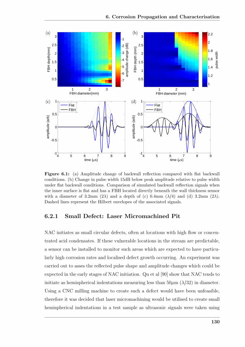
6. Corrosion Propagation and Characterisation
FBH diameter(mm)
FB
H d
ep
th(m
m)
1 2 3
0.5
1
1.5
2
2.5
3
-7
-6
-5
-4
-3
-2
-1
FBH diameter (mm)
FB
H d
ep
th (
mm
)
1 2 3
0.5
1
1.5
2
2.5
3
1
1.2
1.4
1.6
1.8
2
2.2
am
plit
ud
e c
ha
ng
e (
dB
)
pu
lse
wid
th
(a) (b)
4 5 6 7 8 9-1
-0.5
0
0.5
1
time (s)
am
plit
ud
e (
arb
)
Flat
FBH
4 5 6 7 8 9-1
-0.5
0
0.5
1
time (s)
am
plit
ud
e (
arb
)
Flat
FBH
(c) (d)
Figure 6.1: (a) Amplitude change of backwall reflection compared with flat backwallconditions. (b) Change in pulse width 15dB below peak amplitude relative to pulse widthunder flat backwall conditions. Comparison of simulated backwall reflection signals whenthe inner surface is flat and has a FBH located directly beneath the wall thickness sensorwith a diameter of 3.2mm (2λ) and a depth of (c) 0.4mm (λ/4) and (d) 3.2mm (2λ).Dashed lines represent the Hilbert envelopes of the associated signals.
6.2.1 Small Defect: Laser Micromachined Pit
NAC initiates as small circular defects, often at locations with high flow or concen-
trated acid condensates. If these vulnerable locations in the stream are predictable,
a sensor can be installed to monitor such areas which are expected to have particu-
larly high corrosion rates and localised defect growth occurring. An experiment was
carried out to asses the reflected pulse shape and amplitude changes which could be
expected in the early stages of NAC initiation. Qu et al [90] show that NAC tends to
initiate as hemispherical indentations measuring less than 50µm (λ/32) in diameter.
Using a CNC milling machine to create such a defect would have been unfeasible,
therefore it was decided that laser micromachining would be utilised to create small
hemispherical indentations in a test sample as ultrasonic signals were taken using
130

6. Corrosion Propagation and Characterisation
Stage 1 Stage 2 Stage 3
Stage 4 Stage 5
de
pth
(m
m)
(a) (b) (c)
(e) (d) (f)
Figure 6.2: Plan view showing the depth of conical pit during machining during stage(a) 1 (max depth of 100µm) (b) 2 (max depth of 200µm) (c) 3 (max depth of 300µm) (d)4 (max depth of 400µm) (e) 5 (max depth of 500µm). (f) Isometric view of conical pitafter the final stage of machining.
the waveguide transducers. Unlike the experimental setup described in section 3.4,
only two waveguide transducers were used to mimic the actual wall thickness sensor
and ensure sufficient contact pressure could be applied equally between the waveg-
uides to produce signals with high SNR without the need for shear couplant. All
other aspects of the experimental setup remained the same as described in section
3.4.
It was decided that the laser would be used to incrementally ’grow’ a defect directly
below the thickness sensor to simulate NAC initiation. Based on the simulated re-
sults shown in Fig. 6.1, it is clear that a defect diameter of 50µm, two orders of
magnitude smaller than the incident wavelength, would cause almost indistinguish-
able change to the reflected signal. It was therefore assumed that the very earliest
stages would be impossible to detect using the current sensor and the smallest hemi-
spherical indentation to be machined during the experiment would have a diameter
of 200µm. In order to ’grow’ the defect in stages, indentations were machined in
circular loci to form a conical shaped pit over five stages with pit dimensions start-
131

6. Corrosion Propagation and Characterisation
202 202.5 203 203.5 204 204.5-1
-0.5
0
0.5
1
time (s)
Experimental
6 6.5 7 7.5 8 8.5-1
-0.5
0
0.5
1
time (s)
Simulated
Flat
Pitted
202 202.5 203 203.5 204 204.5-1
-0.5
0
0.5
1
time (s)
Experimental
6 6.5 7 7.5 8 8.5-1
-0.5
0
0.5
1
time (s)
Simulated
Flat
Pitted
4 5 6 7 8 9-1
-0.5
0
0.5
1
time (s)
am
plit
ud
e (
arb
)
Flat
FBH
4 5 6 7 8 9-1
-0.5
0
0.5
1
time (s)
am
plit
ud
e (
arb
)
Flat
FBH
0 1 2 3 4 5-0.6
-0.5
-0.4
-0.3
-0.2
-0.1
0
0.1
am
plit
ud
e c
ha
ng
e (
dB
)
pit growth stage
experimental
simulated
(a) (b)
(c)
Figure 6.3: Signal comparison when the backwall is flat and with the largest conical pit(stage 5) for (a) experimental results (b) simulated results. (c) Comparison of amplitudechange calculated using the DPSM simulation and recorded using the thickness sensor forall defect geometries machined during the experiment.
ing with a diameter of 200µm and a depth of 100µm, ending with a diameter of
1400µm and a depth of 500µm. The conical shape was selected to ensure material
would be properly ejected from the test sample during machining and the shape is
a close approximation of what might be expected during the initial stages of NAC.
The depth profile of the five stages of the conical pit are illustrated in figure 6.2 as
predicted using Matlab.
Reflected pulse amplitude has been used in figure 6.3 (c) to track signal change
during the experiment since pulse shape and phase were not seen to vary by any
appreciable amount as illustrated in Fig. 6.3 (a) and (b). It can be seen that
an undulating amplitude pattern exists in Fig. 6.3 (c). Comparison to simulated
results confirmed that it was the way in which the pit was built up using circular
loci of smaller indentations during laser micromachining that caused this amplitude
132

6. Corrosion Propagation and Characterisation
undulation; this effect would not be expected in reality. The largest difference
between experimental and simulated results occur when the sides of the pit are
almost vertical, hinting that this error could be caused by mode conversion effects
not being properly simulated or that point source placement was not optimal during
simulation since gaps between them are largest at these stages. However, the general
trend is predicted well to within 0.17dB at all stages and it can be concluded that
small changes in signal shape can be accurately simulated. Error bars similar to
those shown in Fig. 5.7 have been omitted since a significant change in arrival time
of any part of the pulse is not expected for such small features. This makes the error
associated with the pulse traversing over unwanted modes within the recorded signal
negligible. The extent of observed reflected pulse shape change is so slight in both
experimental and simulated signals that detection of a single small defect within
an industrial environment subject to other forms of signal changing phenomenon
(coupling condition, temperature, incoherent noise, ADC conversion process etc)
would be very challenging.
6.2.2 Large Defect: Flat Bottomed Hole
To enact a large change in signal shape of an amplitude that could be easily detected
in the field a larger defect was selected. Based on the results in Fig. 6.1, a FBH with
a diameter of 3mm was selected as it should show significant amplitude undulation
and pulse width increase. The experimental setup was identical to that in section
6.2.1, other than the defect itself which was machined in 0.1mm depth increments up
to a maximum depth of 3mm using a manual milling machine and a 3mm diameter
end mill cutter. Results from the experiment are shown alongside simulated results
produced by the DPSM simulation in figure 6.4. The signal produced by the DPSM
simulation has been averaged using the method described in section 5.2.1, accounting
for the transduction properties of the waveguide.
A significant change in reflected pulse shape and amplitude can be seen in Fig. 6.4
(a) and (b) from the expected response if the inner surface was flat. Rather than one
distinct pulse, two pulses are recorded; one from the top of the FBH arriving earlier,
and another from the rest of the backwall. It is the interaction between these two
pulses as FBH depth increases which cause the amplitude undulation seen in Fig.
133

6. Corrosion Propagation and Characterisation
200 201 202 203 204 205-1
-0.5
0
0.5
1
time (s)
Experimental
5 6 7 8 9-1
-0.5
0
0.5
1
time (s)
Simulated
Flat
FBH
0 0.5 1 1.5 2 2.5 3-10
-8
-6
-4
-2
0
2
am
plit
ud
e c
ha
ng
e (
dB
)
FBH height (mm)
experimental
simulated
(a) (b)
(c) 4 5 6 7 8 9
-1
-0.5
0
0.5
1
time (s)
am
plit
ud
e (
arb
)
Flat
FBH
4 5 6 7 8 9-1
-0.5
0
0.5
1
time (s)
am
plit
ud
e (
arb
)
Flat
FBH
200 201 202 203 204 205-1
-0.5
0
0.5
1
time (s)
Experimental
5 6 7 8 9-1
-0.5
0
0.5
1
time (s)
Simulated
Flat
FBH
Figure 6.4: Signal comparison when the backwall is flat and with a 3mm diameter FBHwith a depth of 3mm directly below the thickness sensor for (a) experimental results(b) simulated results. (c) Comparison of amplitude change calculated using the DPSMsimulation and recorded using the thickness sensor for all FBH depths. Error bars representthe amplitude error that could be introduced by unwanted modes travelling within thewaveguides which are on average 22dB weaker than the backwall reflection when the innersurface is flat.
(c), a pattern reproduced accurately by the DPSM simulation below an FBH depth
of approximately 1.6mm (λ). As FBH increases still further, low amplitude undula-
tions occur in the experimental results which don’t occur in the simulated case. It
is likely that these are caused by ultrasound which has mode converted into longitu-
dinal waves along the sides of the FBH, interfering with the first backwall reflection
once they have converted back into SH waves during the second reflection with the
inner surface and FBH. The higher velocity of the longitudinal mode cause these
secondary SH waves to arrive earlier than expected, causing increased coherent noise
between the first and second backwall reflections. Even so, the DPSM simulation
predicts amplitude change at all FBH depths to be within expected experimental
error bounds, based upon unwanted wave modes travelling within the waveguides
134
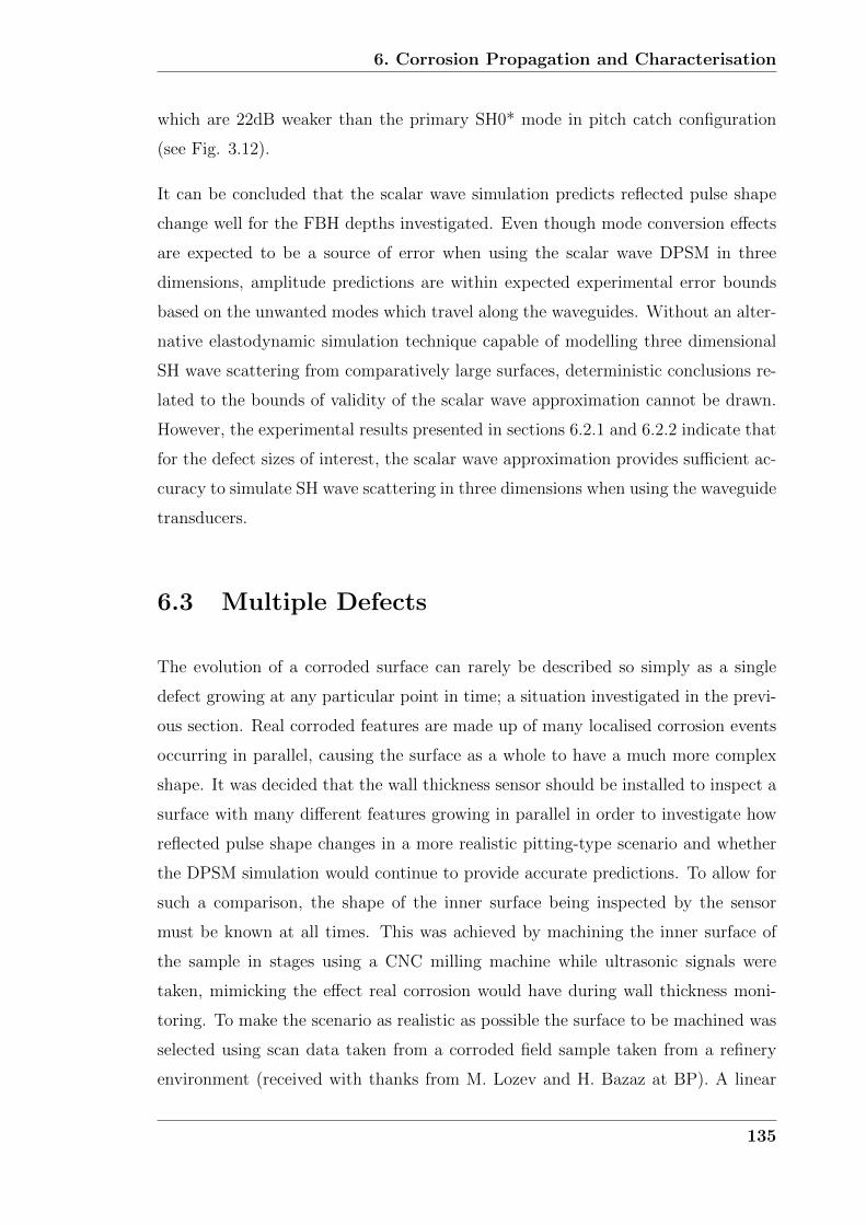
6. Corrosion Propagation and Characterisation
which are 22dB weaker than the primary SH0* mode in pitch catch configuration
(see Fig. 3.12).
It can be concluded that the scalar wave simulation predicts reflected pulse shape
change well for the FBH depths investigated. Even though mode conversion effects
are expected to be a source of error when using the scalar wave DPSM in three
dimensions, amplitude predictions are within expected experimental error bounds
based on the unwanted modes which travel along the waveguides. Without an alter-
native elastodynamic simulation technique capable of modelling three dimensional
SH wave scattering from comparatively large surfaces, deterministic conclusions re-
lated to the bounds of validity of the scalar wave approximation cannot be drawn.
However, the experimental results presented in sections 6.2.1 and 6.2.2 indicate that
for the defect sizes of interest, the scalar wave approximation provides sufficient ac-
curacy to simulate SH wave scattering in three dimensions when using the waveguide
transducers.
6.3 Multiple Defects
The evolution of a corroded surface can rarely be described so simply as a single
defect growing at any particular point in time; a situation investigated in the previ-
ous section. Real corroded features are made up of many localised corrosion events
occurring in parallel, causing the surface as a whole to have a much more complex
shape. It was decided that the wall thickness sensor should be installed to inspect a
surface with many different features growing in parallel in order to investigate how
reflected pulse shape changes in a more realistic pitting-type scenario and whether
the DPSM simulation would continue to provide accurate predictions. To allow for
such a comparison, the shape of the inner surface being inspected by the sensor
must be known at all times. This was achieved by machining the inner surface of
the sample in stages using a CNC milling machine while ultrasonic signals were
taken, mimicking the effect real corrosion would have during wall thickness moni-
toring. To make the scenario as realistic as possible the surface to be machined was
selected using scan data taken from a corroded field sample taken from a refinery
environment (received with thanks from M. Lozev and H. Bazaz at BP). A linear
135

6. Corrosion Propagation and Characterisation
de
pth
(m
m)
z-axis (mm)
x-a
xis
(m
m)
Stage 7
-10 0 10
-10
-5
0
5
10
0
0.5
1
1.5
z-axis (mm)x-a
xis
(m
m)
Stage 14
-10 0 10
-10
-5
0
5
10
0
0.5
1
1.5
z-axis (mm)
x-a
xis
(m
m)
Stage 20
-10 0 10
-10
-5
0
5
10
0
0.5
1
1.5(a) (b) (c)
Figure 6.5: Plan view of the depth of the machined surface directly below the sensor atstage (a) 7 (b) 14 and (c) 20.
progression from flat to fully corroded over 20 stages was used to simulate corrosion
propagation, as well as a 0.05mm uniform depth increase per stage to mimic addi-
tional mean wall loss. A plan view of the depths of three of the surfaces machined
during the course of the experiment as predicted using Matlab are shown in figure
6.5.
The original corroded sample was scanned using a GOM ATOS III Triple Scan white
light scanner which provided point cloud data with higher concentrations of data
points around areas with a low radius of curvature (provided by C.Brett and R.Bell
at E.ON). Interpolation by Kriging [93] was carried out to convert the data points
into a grid format, helping in CAD surface generation and improving simulated result
accuracy obtained using the DPSM. Features with a low radius of curvature on the
original corroded surface were also filtered from the machined surface using a two
dimensional FFT within Matlab to ensure the 2mm diameter ball nose cutter could
machine the required surface profiles. The data retrieval and analysis procedures
remained the same as in section 6.2. Results of the experiment are shown alongside
simulated results in figure 6.6.
The signals shown in Fig. 6.6 (a) and (b) show two main changes to the backwall
reflection from flat to fully ’pitted’; it arrives earlier in time and with reduced
amplitude. The uniform thickness loss of 0.05mm per stage is the predominant
factor in changing the arrival time of the pulse. The corroded shape of the inner
136

6. Corrosion Propagation and Characterisation
200 201 202 203 204 205
-1
-0.5
0
0.5
1
time (s)
Experimental
5 6 7 8 9
-1
-0.5
0
0.5
1
time (s)
Simulated
Flat
Pitted
0 2 4 6 8 10 12 14 16 18 20-5
-4
-3
-2
-1
0
1
2
am
plit
ud
e c
ha
ng
e (
dB
)
machined stage
experimental
simulated
200 201 202 203 204 205
-1
-0.5
0
0.5
1
time (s)
Experimental
5 6 7 8 9
-1
-0.5
0
0.5
1
time (s)
Simulated
Flat
Pitted
(a) (b)
4 5 6 7 8 9-1
-0.5
0
0.5
1
time (s)
am
plit
ud
e (
arb
)
Flat
FBH
4 5 6 7 8 9-1
-0.5
0
0.5
1
time (s)
am
plit
ud
e (
arb
)
Flat
FBH
(c)
Figure 6.6: Signal comparison when the backwall is flat and the final stage of corrosionmachining (stage 20) for (a) experimental results (b) simulated results. (c) Comparison ofamplitude change calculated using the DPSM simulation and recorded using the thicknesssensor for all machined corrosion stages. Error bars represent the amplitude error thatcould be introduced by unwanted modes travelling within the waveguides which are onaverage 22dB weaker than the backwall reflection when the inner surface is flat.
surface enhances scattering of the pulse, directing ultrasonic energy away from the
receiver, therefore reducing the amplitude of the recorded pulse as the severity of
the pitting increases. Referring to Fig. 6.6 (c), the amplitude of the pulse again
undulates as the machined surfaces become deeper. The size of this undulation is
consistent with unwanted modes travelling within the waveguides; as the reflected
pulse traverses the recorded signal during thickness reduction, it constructively and
destructively interferes with these lower amplitude modes. The simulated results
are within these expected errors, indicating that the scalar wave DPSM performs
well on reflecting surfaces made up of many localised features without the need for
a more complex elastodynamic wave approach. The reflected pulse shape changes
observed for this pitted surface are consistent with the level of change seen when
considering rough surfaces with Gaussian height and length characteristics. It is
137

6. Corrosion Propagation and Characterisation
expected that the conclusions drawn within Chapters 4 and 5 are therefore applicable
when considering corroded surfaces made up of more localised features with similar
RMS heights and length characteristics.
6.4 Corrosion Propagation
The process by which a rough or corroded surface attains its particular shape has
been largely ignored so far in this thesis. A linear progression from flat to fully cor-
roded where all features grow in parallel with the same rate was assumed in section
6.3; however, this is unlikely to be the true manner in which the corroded surface was
originally formed during corrosion. The aim of this section is to investigate a more
realistic material loss mechanism in order to evaluate the corrosion rate estimation
capabilities for each of the TOF algorithms described in section 4.3.1.
6.4.1 Simulated Corrosion
Extensive amounts of literature exist describing different corrosion mechanisms and
the varied ways in which their propagation can be simulated or statistically pre-
dicted. A full review was considered outside the scope of this thesis and as such
only the relevant theory for the model implemented will be described in any detail.
For more information on alternative pitting corrosion models used in the oil and gas
industries please see [94–99].
The model proposed by Meakin et al [100] was chosen because it is relatively simple
to implement and it focusses specifically on the morphology of localised pit-type
defects, describing the structure of the corrosion front as the defect develops. It
describes both uniform (smooth brightening pits) and non-uniform (rough ’etching’
pits) corrosion processes by introducing passivation and depassivation rates which
act to change the characteristics of material at specific sites within the simulated
domain. It is based on a two dimensional cross-section of the material being sub-
divided into a square lattice in which each site in the lattice can be one of four
different states:
138

6. Corrosion Propagation and Characterisation
1. Unreactive fluid (empty).
2. Corrosive fluid or particle.
3. Reactive metal.
4. Passive non-reactive metal.
Corrosion is assumed to be the result of a diffusion limited reaction between mobile
corrosive sites and the unprotected metal surface. The mobile corrosive sites are
controlled using a random walk algorithm which causes them to come into contact
with metal along the corrosion front. If the site is reactive then the two reagents
combine and the site becomes unreactive fluid, therefore causing material loss. If
the site is passive nothing happens and the corrosive site stays where it was to
be moved to another potentially reactive metal site along the corrosion front. To
establish non-uniform pit growth spontaneous random events are introduced which
are characterised by the passivation and depassivation rate constants (kp and kd
respectively). The passivation rate controls whether previously reactive metal sites
along the corrosion front spontaneously become passive and the depassivation rate
controls whether previously passive sites along the corrosion front spontaneously
becomes reactive again. Two pits are shown in figure 6.7 to illustrate the difference
between pit shapes caused by uniform and non-uniform pit growth, controlled using
these parameters. The time variable is arbitrary and controlled using the number of
corrosive site movements per unit time. Singular pits were generated in these cases
by only allowing corrosive sites to enter through a single empty site on the inner
surface.
A three dimensional approach was deemed unnecessary during this initial investi-
gation into corrosion rate estimation capabilities of the TOF algorithms because of
the large increase in computational resources and time which would otherwise be
required. Using two dimensional DPSM in conjunction with the pitting simulation
(also written using Matlab) allowed simulated ultrasonic signals from many corrod-
ing surfaces to be acquired very rapidly. The results should therefore be taken as a
worst case scenario as it is expected that diffuse components of the reflected pulse
will be amplified by of a lack of spatial averaging in two dimensions, as was the case
with Gaussian distributed roughness shown in Chapter 5.
139

6. Corrosion Propagation and Characterisation
kp =0.1e
-3, k
d = 100e
-6, time = 9000
x-axis (mm)
y-a
xis
(m
m)
-2 -1 0 1 20
0.5
1
1.5
2
kp =3e
-3, k
d = 1e
-6, time = 9000
x-axis (mm)
y-a
xis
(m
m)
-2 -1 0 1 20
0.5
1
1.5
2
Reactive metal Reactive metal on corrosion front
Passive site Corrosive site Unreactive fluid
(a) (b)
Figure 6.7: Examples of single pits resulting from conditions of (a) uniform growth (b)non-uniform growth.
6.4.2 Corrosion Rate Estimation
To simulate behaviour similar to the interaction between SC and NAC during real
corrosion where both uniform was loss and localised defects occur, it was decided
that initially all sites on the corrosion front would be reactive and kp and kd would be
used to alter corrosion propagation through time. Initially uniform wall loss occurs,
representing a situation where SC is dominant; however, as corrosion proceeds and
passive sites begin to appear, so too do localised features representing a change to
a more NAC dominated scenario. For a grid size of 100µm, values of kp = 0.25e−3
and kd = 100e−6 were found to produce the desired corrosion characteristics up to a
mean wall loss of 1mm (10%), beyond which the passivation rate halted corrosion
almost entirely. The mean wall loss was defined as the area of material lost below the
corrosion front divided by the horizontal length of the surface being corroded. The
DPSM simulation calculated signals at 50 stages during the corrosion of a particular
surface, each separated by 0.02mm mean wall loss. The random numbers used to
generate the trajectories of the corrosive sites were altered to produce different
corroding surfaces, 950 of which were simulated. An example of a corroding surface
produced by the pitting simulation is shown in figure 6.8, alongside the signals
calculated using the DPSM simulation. More results have been shown for greater
levels of wall loss because of the greater surface RMS height and associated signal
distortion.
140

6. Corrosion Propagation and Characterisation
-4 -2 0 2 4
0
1
2
time = 1.8, mean wall loss = 0.0705mm
x-axis (mm)
y-a
xis
(m
m)
-4 -2 0 2 4
0
1
2
time = 57.4, mean wall loss = 0.5505mm
x-axis (mm)
y-a
xis
(m
m)
-4 -2 0 2 4
0
1
2
time = 147.6, mean wall loss = 0.79mm
x-axis (mm)
y-a
xis
(m
m)
-4 -2 0 2 4
0
1
2
time = 232.3, mean wall loss = 0.9mm
x-axis (mm)
y-a
xis
(m
m)
-4 -2 0 2 4
0
1
2
time = 342.8, mean wall loss = 0.97mm
x-axis (mm)
y-a
xis
(m
m)
-4 -2 0 2 4
0
1
2
time = 394.3, mean wall loss = 1mm
x-axis (mm)
y-a
xis
(m
m)
5 6 7 8 9 10
-0.1
0
0.1
am
plitu
de
(P
a)
time (s)
5 6 7 8 9 10
-0.1
0
0.1
am
plitu
de
(P
a)
time (s)
5 6 7 8 9 10
-0.1
0
0.1
am
plitu
de
(P
a)
time (s)
5 6 7 8 9 10
-0.1
0
0.1
am
plitu
de
(P
a)
time (s)
5 6 7 8 9 10
-0.1
0
0.1
am
plitu
de
(P
a)
time (s)
5 6 7 8 9 10
-0.1
0
0.1
am
plitu
de
(P
a)
time (s)
(a.i)
(a.ii)
(b.i)
(b.ii)
(c.i)
(c.ii)
(d.i)
(d.ii)
(e.i)
(e.ii)
(f.i)
(f.ii)
Flat Pitted Flat Pitted Flat Pitted
Flat Pitted Flat Pitted Flat Pitted
Flat
Pitted
Flat
Pitted
Flat
Pitted
Flat
Pitted
Flat
Pitted
Flat
Pitted
Figure 6.8: Example of a corroding backwall shown alongside the simulated pulse re-flected from the surface calculated using the DPSM for a mean wall loss of (a) 0.07mm(b) 0.55mm (c) 0.79mm (d) 0.9mm (e) 0.97mm and (f) 1mm.
The surface profiles of the corroding surface initially have low RMS height and the
localised defects tend to be small as they are made up of only a few squares of the
material lattice. However, it can be seen in Fig. 6.8 that as corrosion proceeds,
the height and length characteristics of localised features increase because passive
sites restrict growth from occurring uniformly along the surface. The associated re-
flected pulse distortion also tends to increase as these features grow in size, therefore
impacting on the behaviour of the TOF algorithms. Each algorithm (as described
in section 4.3.1) was applied to all the signals produced by this particular corrod-
ing surface and the results are shown in figure 6.9, alongside the linear corrosion
gradient estimations. In this idealised case where the material loss within the wall
is accurately known, a corrosion gradient has been used rather than a corrosion
rate in order to remove any influence of the arbitrary time variable used within the
corrosion model. The corrosion gradient is defined as the estimated wall loss over
the actual mean wall loss; therefore a value of 1 corresponds to the TOF algorithm
141

6. Corrosion Propagation and Characterisation
9 9.5 10
8.6
8.8
9
9.2
9.4
9.6
9.8
10
10.2
mean wall thickness (mm)
estim
ate
d w
all
thic
kn
ess (
mm
)
MIN
MEAN
MAX
EP
XC
FA
9 9.5 10
8.6
8.8
9
9.2
9.4
9.6
9.8
10
10.2
mean wall thickness (mm)
estim
ate
d w
all
thic
kn
ess (
mm
)
MEAN
EP
XC
FACODEP=0.20
CODXC=0.25
CODFA=0.95
(a) (b)
Figure 6.9: (a) Comparison of estimated wall thickness trends for envelope peak de-tection (EP), cross-correlation (XC) and threshold first arrival (FA) TOF algorithm. A15dB threshold was used for FA. Lines have been included showing the actual minimum,maximum and mean wall thickness of the surface calculated using the surface profiles. (b)Comparison of linear regression lines and their associated COD values for each TOF algo-rithm. The data points show the wall thickness estimates from which the linear regressionlines have been calculated.
finding the mean wall loss exactly. The value of the coefficient of determination
(COD) has also been included for each TOF algorithm in Fig. 6.9 (b) to indicate
how well the linear regression lines fit the estimated wall thickness data; a value of
1 corresponding to a perfect linear fit and a value of 0 to zero shape similarity.
A discontinuity in thickness estimate occurs for both envelope peak detection and
cross-correlation, caused by signal amplitude in the tail of the pulse exceeding that
of the main pulse. If included in the linear regression, such discontinuities can have
a large impact on corrosion gradient estimates, which for envelope peak detection
and cross-correlation were 0.50 and 0.52 respectively. The COD values also indi-
cate the very low correlation between the linear regression and observed thickness
trends. Threshold first arrival is not as sensitive to energy in the tail of the reflected
pulse, therefore it is found to perform far better, calculating a corrosion gradient of
0.99 with a COD of 0.95. Values for the COD and corrosion gradient for all 950
corrosion simulations carried out are shown in figure 6.10 (a) and (b) respectively.
It can be seen that because threshold first arrival is not affected so strongly by
142
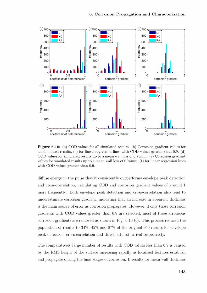
6. Corrosion Propagation and Characterisation
0 1 20
200
400
600
800
corrosion gradient
fre
qu
en
cy
EP
XC
FA
0 1 20
100
200
300
400
500
600
700
corrosion gradient
fre
qu
en
cy
EP
XC
FA
0 1 20
100
200
300
400
500
600
700
corrosion gradient
fre
qu
en
cy
EP
XC
FA
0 1 20
200
400
600
800
corrosion gradient
fre
qu
en
cy
EP
XC
FA
0 0.5 10
100
200
300
400
500
600
700
coefficeint of determination
fre
qu
en
cy
EP
XC
FA
(a) (b) (c)
0 0.5 10
200
400
600
800
coefficeint of determination
fre
qu
en
cy
EP
XC
FA
(d) (e) (f)
Figure 6.10: (a) COD values for all simulated results. (b) Corrosion gradient values forall simulated results, (c) for linear regression lines with COD values greater than 0.9. (d)COD values for simulated results up to a mean wall loss of 0.75mm. (e) Corrosion gradientvalues for simulated results up to a mean wall loss of 0.75mm, (f) for linear regression lineswith COD values greater than 0.9.
diffuse energy in the pulse that it consistently outperforms envelope peak detection
and cross-correlation, calculating COD and corrosion gradient values of around 1
more frequently. Both envelope peak detection and cross-correlation also tend to
underestimate corrosion gradient, indicating that an increase in apparent thickness
is the main source of error as corrosion propagates. However, if only those corrosion
gradients with COD values greater than 0.9 are selected, most of these erroneous
corrosion gradients are removed as shown in Fig. 6.10 (c). This process reduced the
population of results to 34%, 45% and 87% of the original 950 results for envelope
peak detection, cross-correlation and threshold first arrival respectively.
The comparatively large number of results with COD values less than 0.9 is caused
by the RMS height of the surface increasing rapidly as localised features establish
and propagate during the final stages of corrosion. If results for mean wall thickness
143

6. Corrosion Propagation and Characterisation
losses greater than 0.75mm are omitted during the corrosion gradient calculation
(corresponding to RMS heights greater than approximately 0.1mm), these large
jumps in thickness rarely affect the final result. This is evident in Fig. 6.10 (d)
where almost all COD values are above 0.95 for threshold first arrival and cross-
correlation. Envelope peak detection also improves; however the majority of the
linear regression lines have a value between 0.85 and 0.95, indicating that the TOF
algorithm is the least accurate of the three tested. This is also clearly illustrated in
Fig. 6.10 (e) where the distribution of corrosion gradients is spread more widely than
for both cross-correlation and threshold first arrival. By ignoring wall losses greater
then 0.75mm, cross-correlation is now found to be more precise than threshold first
arrival, indicated by a tighter distribution around the correct corrosion gradient.
Both show a positive skew, tending to slightly overestimate corrosion gradient, a
situation which is more favourable than the reverse in a safety critical oil refinery
environment.
Coupled with the results presented in Chapter 4, the main conclusions that can
be drawn from these simulated results which are free from other forms of noise
are that under low RMS height conditions where rapid changes in estimated wall
thickness are not expected, cross-correlation would be the optimum method for
calculating corrosion rates. If however large jumps in thickness are observed, TOF
algorithms based on the earliest arrival time of a pulse would be the most stable.
As such, for operation in the field a combination of both should be implemented to
ensure maximum precision during the early stages of corrosion and the best possible
accuracy during the later stages of severe corrosion. Other methods of detecting
and removing large jumps in estimated thickness could also be implemented to
improve corrosion rate estimation such as alternative regression models or roughness
detection as an indicator of ongoing and potentially severe corrosion.
6.5 Inverse Scattering with Limited Data
It has already been shown in section 4.2.2 that reconstructing a rough surface using
information contained in the only A-scan available at any particular time during
permanent wall thickness monitoring would be impossible. It could be possible
144

6. Corrosion Propagation and Characterisation
using a lookup table type method if assumptions could be made about the form of
the features on the inner surface causing the pulse to change shape; however, as
the previous sections have described, corroded features are rarely fully predictable
in shape. This leaves only one option: tracking how pulse shape changes through
time as corrosion propagates. Such a method could also provide a means of advising
when operation should switch from one type of TOF algorithm to another.
Referring back to the work presented in section 4.4, it was found that calculating
the correlation coefficient between the transmitted and received pulse provided the
most promising method of measuring the extent of reflected pulse shape change
and the impact this can have on estimated thickness error. It could therefore also
be used to track signal shape change through time in order to provide information
on how the condition of the surface deteriorates as corrosion proceeds. This has
been carried out for the corroding surface shown in Fig. 6.8 as an example, shown
alongside the mean change in correlation coefficient for all 950 simulated cases as
corrosion propagates in figure 6.11. It can be seen that for an individual surface that
the correlation coefficient of the reflected pulse can alter quite substantially through
time, both increasing and decreasing as the reflected signal alters to become more or
less similar in shape to the ideal transmitted pulse. Over many corroding surfaces
these variations average out and the decrease in correlation coefficient mirrors how
the average RMS height of the corroding surfaces increases. It should be noted that
the average results shown in Fig. 6.11(b) and are only included to illustrate the
most common trends; the change in correlation coefficient for individual surfaces
can vary substantially from this result as illustrated in Fig. 6.11(a).
The results shown in Fig. 6.11 (b) should be treated with caution since any par-
ticular rough surface will have its own unique trend, not necessarily showing a sub-
stantial decrease in correlation coefficient even with a large increase in RMS height.
Furthermore, applying the technique directly to real signals can have added com-
plications. To illustrate these points the correlation coefficients of the experimental
signals presented in section 5.3.2 have been calculated and are shown in figure 6.12.
These particular experimental results were chosen because of the substantial change
in signal shape exhibited as RMS height increases and the comparison which can
be made from signals reflecting from the same surface but recorded at locations
145
6. Corrosion Propagation and Characterisation
8.8 9 9.2 9.4 9.6 9.8 100.8
0.85
0.9
0.95
1
8.8 9 9.2 9.4 9.6 9.8 100
0.05
0.1
0.15
0.21
0.95
0.9
0.85
0.8 9 9.2 9.4 9.6 9.8 10
0.2
0.15
0.1
0.05
0
mean wall thickness (mm)
co
rre
latio
n c
oe
ffic
ien
t
RM
S h
eig
ht (m
m)
8.8 9 9.2 9.4 9.6 9.8 1010
0.5
0.6
0.7
0.8
0.9
1
mean wall thickness (mm)
co
rre
latio
n c
oe
ffic
ien
t
10 8.8
(a) (b)
Figure 6.11: (a) Correlation coefficient of simulated signals as pitting corrosion proceedsfor example surface. (b) Average correlation coefficient and RMS height as corrosionproceeds over 950 surfaces.
separated by only 2mm (1.25λ).
The first conclusion that can be drawn from experimental results is that even under
flat backwall conditions, the correlation coefficient is not equal to 1. This is because
the ideal transmitted pulse which has been compared with is free from any noise,
whereas even the best quality experimental signal is subject to noise, most notably
caused by unwanted modes travelling within the waveguides. To correct this, the
initial experimental signal could be used instead of the ideal transmitted pulse;
therefore subsequent comparison will indicate change from the initial state now
corresponding to a correlation coefficient value of 1. However, when using an ideal
pulse for comparison, any increase in correlation coefficient value from the sensors
initial state could be an indicator of improving coupling conditions, for example
when temperature cycling ensues. Comparison to a less ideal state in this case would
undermine the usefulness of the technique, therefore it is advised that comparison
should always be made to the ideal transmitted signal and changes in correlation
coefficient should be monitored as an indication of signal quality and the potential
onset of severe corrosion. Not being able to use absolute values of the correlation
coefficient in the field does however mean that direct use of the uncertainty plots
presented in section 4.4.2 would be unadvisable. In cases where severe corrosion
146
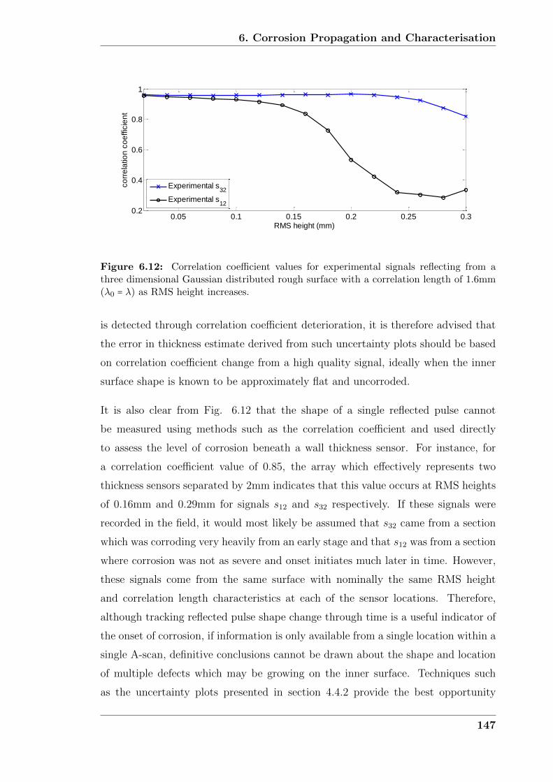
6. Corrosion Propagation and Characterisation
0.05 0.1 0.15 0.2 0.25 0.30.2
0.4
0.6
0.8
1
RMS height (mm)
co
rre
latio
n c
oe
ffic
ien
t
Experimental s32
Experimental s12
Figure 6.12: Correlation coefficient values for experimental signals reflecting from athree dimensional Gaussian distributed rough surface with a correlation length of 1.6mm(λ0 = λ) as RMS height increases.
is detected through correlation coefficient deterioration, it is therefore advised that
the error in thickness estimate derived from such uncertainty plots should be based
on correlation coefficient change from a high quality signal, ideally when the inner
surface shape is known to be approximately flat and uncorroded.
It is also clear from Fig. 6.12 that the shape of a single reflected pulse cannot
be measured using methods such as the correlation coefficient and used directly
to assess the level of corrosion beneath a wall thickness sensor. For instance, for
a correlation coefficient value of 0.85, the array which effectively represents two
thickness sensors separated by 2mm indicates that this value occurs at RMS heights
of 0.16mm and 0.29mm for signals s12 and s32 respectively. If these signals were
recorded in the field, it would most likely be assumed that s32 came from a section
which was corroding very heavily from an early stage and that s12 was from a section
where corrosion was not as severe and onset initiates much later in time. However,
these signals come from the same surface with nominally the same RMS height
and correlation length characteristics at each of the sensor locations. Therefore,
although tracking reflected pulse shape change through time is a useful indicator of
the onset of corrosion, if information is only available from a single location within a
single A-scan, definitive conclusions cannot be drawn about the shape and location
of multiple defects which may be growing on the inner surface. Techniques such
as the uncertainty plots presented in section 4.4.2 provide the best opportunity
147

6. Corrosion Propagation and Characterisation
for data extraction in applications such as wall thickness monitoring since they
provide probabilistic rather than deterministic estimates of corrosion induced errors
in situations where data is very limited.
It is important to note that these conclusions have been drawn from worst case
scenarios, be it from two dimensional simulated results or experimental results where
the surface was specifically chosen to show signal disparity between neighboring
sensor positions. It is expected that the majority of cases seen in the field will
show reduced levels of reflected pulse shape change and the thickness estimates they
produce will be less sensitive to the levels of corrosion expected within petrochemical
refinery environments.
6.6 Summary
Building upon the work presented in previous chapters which investigated ultra-
sound reflection from rough surfaces with Gaussian height and length characteris-
tics, alternative defect morphologies and growth mechanisms have been investigated.
Simplified geometries such as a FBH showed that a single localised defect could in-
fluence reflected pulse shape greatly, changing amplitudes by up to 8dB for defect
sizes up to 2λ. Comparison of experimental and simulated results for a micron-scale
laser micromachined conical pit-like defect and a 3mm diameter FBH indicated that
the scalar wave approach predicted amplitude trends closely, within the expected er-
rors introduced by imperfect mode purity in the waveguide transducers. Without an
alternative three dimensional elastodynamic simulation technique, the experimental
results indicated that the scalar wave DPSM is sufficiently accurate to simulate SH
wave scattering from pit-like features of comparable size to the incident wavelength
using the waveguide transducers.
More realistic defect geometries and propagation mechanisms were investigated
through experimental and simulated studies. Scan data taken from a real sample
taken from a corrosive refinery environment was used to machine a pitted surface
below a wall thickness sensor which was linearly increased in height to approximate
increasingly corroded conditions. The change in pulse shape as the experiment pro-
148

6. Corrosion Propagation and Characterisation
gressed was found to be consistent with that found in Chapter 5, suggesting that
conclusions drawn about ultrasound reflection from rough surfaces with Gaussian
height and length characteristics are equally valid for those subject to pitting cor-
rosion with comparable feature sizes. A two dimensional simulation based on a
diffusion limited reaction was implemented to more closely approximate how ma-
terial is lost during pitting corrosion; simulated signals were subsequently calcu-
lated at each stage using the DPSM. Corrosion rates calculated using the envelope
peak detection, cross-correlation and threshold first arrival TOF algorithms echo
the conclusions made for discrete wall thickness calculations in Chapter 4; for se-
vere corrosion, algorithms based on determining the earliest arrival of a pulse are
more stable, otherwise cross-correlation is found to be the most accurate, providing
precise corrosion rate estimates.
Based on the results found, some recommendations about algorithm deployment
in the field have been provided. Primarily, reliance on a single TOF algorithm is
unadvisable as each can be affected by corrosion in different ways; a better strategy
is to employ cross-correlation and threshold first arrival and track how the estimated
corrosion rates change through time. A large difference between them is a likely to
indicate the onset of severe corrosion and results given by threshold first arrival
should be taken as the most stable. Measuring how pulse shape changes through
time using methods such as the correlation coefficient provides a useful probabilistic
indicator of corroded feature development on the inner surface, and therefore the
reliability of the estimated thickness. However, with only a single ultrasonic signal
to extract information from, definitive conclusions about the true nature of the
inner surface cannot be drawn. Application of an array of waveguides within a high
temperature environment would increase the information content about a defect,
allowing more deterministic conclusions to be drawn about its size and location.
This situation will be the focus of the next chapter.
149

Chapter 7
Alternative Remote Monitoring
Methods using Waveguide Arrays
7.1 Introduction
Previous chapters have focused on monitoring material degradation and corrosion
by measuring localised wall thickness loss using a sensor made up of two ultrasonic
waveguide transducers setup in pitch-catch configuration. The comparative lack
of information available in a single signal from a single location makes determinis-
tic conclusions about the exact nature of the reflecting surface impossible to draw.
Methods to increase positional data content such as probe scanning are not possi-
ble in permanent monitoring applications, therefore the only approach to increase
positional information is by means of an array, allowing defects to be interrogated
from multiple directions.
In the following sections two of the most promising structural degradation moni-
toring applications which have been identified as benefitting from the increase in
data available from an array of waveguides will be presented. The first is monitor-
ing thermal fatigue crack growth within a high temperature, high pressure steam
power plant environment. It will be shown that the additional data can be manip-
ulated to create an image of a crack, indicating both position and length relative
to the array. Simulated studies are carried out in order to define the working en-
150

7. Alternative Remote Monitoring Methods using Waveguide Arrays
velope of the array, with comparison to experimental results providing validation of
hardware design and prototype readiness for industrial implementation. The second
application investigates how a two dimensional velocity distribution can be recon-
structed using ultrasonic data in order to isolate areas of material degradation such
as hydrogen attack which can alter bulk material properties. A proof-of-concept
experimental investigation was carried out using a transient heat distribution to
simulate the effect such corrosion mechanisms could have, providing feedback on
velocity change detectability limits, as well as the positional resolution of a limited
view array geometry.
7.2 Thermal Fatigue Crack Growth Monitoring
The way in which power plants are operated throughout the UK has changed a great
deal in the past few decades. Deregulation has led to plants which were originally
designed to operate under base load conditions to endure far more frequent load
changes and start cycles (known as two-shifting) in order to match supply with
fluctuating demand in a competitive energy market. This increase in load cycles,
coupled with the age of many plants has caused circumferential thermal fatigue
cracks to grow in the chrome moly vanadium (CMV) steel steam pipework butt
welds [7]. Left unchecked these cracks could grow to the point of failure, presenting
a safety hazard and incurring large maintenance and repair costs.
Upon discovering such defects, conventional ultrasonic inspection has been employed
to measure their extent in an attempt to monitor their development, and to provide
stress analysts with information vital in deciding whether a plant is safe to operate
in its current condition. However, because conventional ultrasonic transducers can-
not withstand elevated temperatures, current inspection techniques can only occur
when the plant is shut down during planned maintenance cycles which generally
occur years apart. This leads to poor repeatability because of the potential for
operator, equipment and positioning variance. Furthermore, crack undersizing due
to tip closure can occur at low temperature [101]. An improved strategy would be
to permanently monitor small, subcritical cracks that have been identified during
routine inspection. This would allow more accurate and repeatable evaluation of
151

7. Alternative Remote Monitoring Methods using Waveguide Arrays
the defect size, prevention of unplanned shut downs due to component failure and
more efficient scheduling of component replacements, all of which increase plant
availability and hence maximise revenue.
Currently, permanently installable ultrasonic crack monitoring devices that can sur-
vive high temperatures (above 200○C) are not commercially available and the con-
struction of such a device has formed the motivation for the work presented in this
section. Much of the work presented has previously been reported in our papers
[102] and [103], as such some relevant excerpts have been included in section 7.2.
7.2.1 Fatigue Crack Monitoring Strategy
Many techniques can be used to measure the size of a crack using ultrasonic waves.
The most commonly used method is time of flight diffraction (TOFD) [104–106].
Such applications usually employ longitudinal waves which diffract strongly from
crack tips. By scanning two transducers of fixed separation across the outer surface
of a component containing a crack, simple geometric considerations can be used to
size the crack based on the arrival time of the diffracted signal. The advantage of
this monitoring strategy is that only two transducers are needed to size the crack;
however, as described by Chapman [107], the expression for the far field diffracted
amplitude A of a plane SH wave within an infinite medium incident upon a semi-
infinite planar crack is given by:
A(θ) =cos2(θ/2)
2πcos(θ)eiπ/4
√λ
reikr (7.1)
Where the incident and reflected angles are assumed to be equal (θ) and r is the
observation distance. If this equation is plotted as shown in figure 7.1 it is clear
that the amplitude of the diffracted SH wave would be below the detectability limit
(often around -40dB for standard equipment) when inspecting at angles greater than
130○. This is the case when the transducers are installed on the outer surface of the
component inspecting a crack initiating on the inner surface, such as would be the
case in a steam power plant environment. Experimental studies were carried out to
verify TOFD would be unsuitable using the waveguide transducers, the details of
152

7. Alternative Remote Monitoring Methods using Waveguide Arrays
0 50 100 150-100
-80
-60
-40
-20
0
no
rma
lise
d S
H w
ave
am
plit
ud
e (
dB
)
angle ()
θ θ
(a) (b)
crack tip
crack
incident
wave
Figure 7.1: (a) Geometry considered for diffraction of a plane wave from a crack tip whenthe incident angle θ is equal to the receiving angle. (b) Diffracted SH wave amplitude whenthe observation distance (r) is 30mm and λ=1.6mm. The dashed line represents the typicalsignal to noise ratio for standard equipment (-40dB).
which can be found in our paper [103].
An alternative monitoring strategy is to use waves which have reflected from the
crack face via the backwall. Termed the multi-synthetic aperture focussing technique
(multi-SAFT) [108, 109], it takes advantage of higher amplitude components being
received by an array of waveguides caused by lower incidence angles. The received
waveforms can subsequently be used to construct an image of the crack based on the
distance travelled from the transmitter to the receiver via the backwall and crack
face. These distances are calculated using equations 7.2 and 7.3 assuming a plate
geometry with thickness T .
dtx =√
(xtx − x)2 + (T + (T − y))2 (7.2)
drx =√
(xrx − x)2 + y2 (7.3)
where subscript tx refers to the transmitter and subscript rx refers to the receiver.
Once a full matrix capture (FMC) data set is acquired, the total focussing method
(TFM) [110] can be used to construct the image I(x, y) of the crack using equation
7.4.
I(x, y) = ∣∑tx∑rx
gtx,rx(dtxc+drxc
)∣ (7.4)
153

7. Alternative Remote Monitoring Methods using Waveguide Arrays
Depth = 4.9mm
x-axis (mm)
y-a
xis
(m
m)
0 10 20-30
-25
-20
-15
-10
-5
0
-20
-15
-10
-5
0
y
x
dtx
drx
SH wave transmitters and receivers
crack offset
crack length
image area (a) (b)
ima
ge
am
plit
ud
e (
dB
)
Figure 7.2: (a) Array geometry considered showing the path analyzed during TFMimaging. (b) Example TFM image calculated using simulated signals.
Where gtx,rx(t) is the time dependent signal recorded at transducer rx when trans-
ducer tx is transmitting. Areas in the image which have a high amplitude represent
areas in the original geometry which have strong reflections associated with them
based on the sum of the propagation distances given by equations 7.2 and 7.3. The
TFM was used because it uses data from all possible combinations of transmit-
receive waveguide pairings when creating an image, requiring no predetermined fo-
cussing laws or complicated electronics. A schematic of the inspection geometry is
shown in figure 7.2, alongside an example image of a crack calculated using simulated
data. It should be noted that the axis system is different from previous chapters in
this thesis since it was decided the crack position should be calculated relative to
the first element in the waveguide array.
7.2.2 Simulated Investigation of Array Working Envelope
The two dimensional scalar wave DPSM simulation described in Chapter 3 for mod-
elling rough surface scattering is equally valid when simulating SH wave scattering
from a crack-like defect which is constant in cross-section across the width of the
array. As such the theory will not be repeated here; however, one important sim-
plifying assumption was made to improve simulation efficiency in this particular
application since N2 signals are needed to simulate a FMC data set for an array
made up of N waveguides. In order to reduce the number of passive sources, the
154
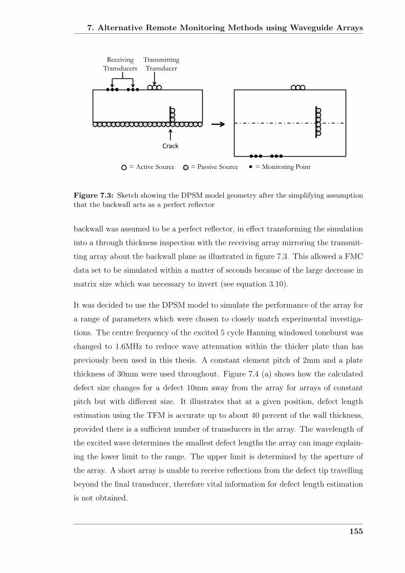
7. Alternative Remote Monitoring Methods using Waveguide Arrays
= Active Source = Passive Source = Monitoring Point
Transmitting
Transducer
Receiving
Transducers
Crack
Figure 7.3: Sketch showing the DPSM model geometry after the simplifying assumptionthat the backwall acts as a perfect reflector
backwall was assumed to be a perfect reflector, in effect transforming the simulation
into a through thickness inspection with the receiving array mirroring the transmit-
ting array about the backwall plane as illustrated in figure 7.3. This allowed a FMC
data set to be simulated within a matter of seconds because of the large decrease in
matrix size which was necessary to invert (see equation 3.10).
It was decided to use the DPSM model to simulate the performance of the array for
a range of parameters which were chosen to closely match experimental investiga-
tions. The centre frequency of the excited 5 cycle Hanning windowed toneburst was
changed to 1.6MHz to reduce wave attenuation within the thicker plate than has
previously been used in this thesis. A constant element pitch of 2mm and a plate
thickness of 30mm were used throughout. Figure 7.4 (a) shows how the calculated
defect size changes for a defect 10mm away from the array for arrays of constant
pitch but with different size. It illustrates that at a given position, defect length
estimation using the TFM is accurate up to about 40 percent of the wall thickness,
provided there is a sufficient number of transducers in the array. The wavelength of
the excited wave determines the smallest defect lengths the array can image explain-
ing the lower limit to the range. The upper limit is determined by the aperture of
the array. A short array is unable to receive reflections from the defect tip travelling
beyond the final transducer, therefore vital information for defect length estimation
is not obtained.
155
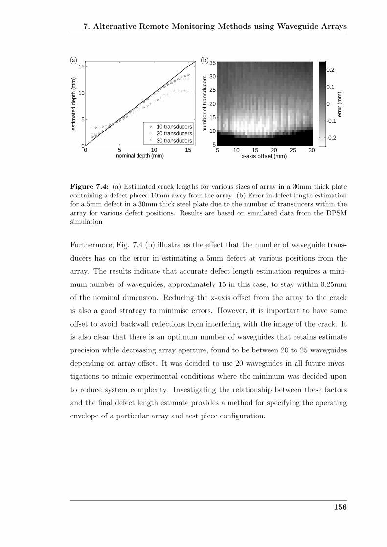
7. Alternative Remote Monitoring Methods using Waveguide Arrays
x-axis offset (mm)
num
ber
of tr
ansducers
5 10 15 20 25 305
10
15
20
25
30
35
-0.2
-0.1
0
0.1
0.2
0 5 10 150
5
10
15
nominal depth (mm)
estim
ate
d d
epth
(m
m)
10 transducers
20 transducers
30 transducers
err
or
(mm
)
(a) (b)
Figure 7.4: (a) Estimated crack lengths for various sizes of array in a 30mm thick platecontaining a defect placed 10mm away from the array. (b) Error in defect length estimationfor a 5mm defect in a 30mm thick steel plate due to the number of transducers within thearray for various defect positions. Results are based on simulated data from the DPSMsimulation
Furthermore, Fig. 7.4 (b) illustrates the effect that the number of waveguide trans-
ducers has on the error in estimating a 5mm defect at various positions from the
array. The results indicate that accurate defect length estimation requires a mini-
mum number of waveguides, approximately 15 in this case, to stay within 0.25mm
of the nominal dimension. Reducing the x-axis offset from the array to the crack
is also a good strategy to minimise errors. However, it is important to have some
offset to avoid backwall reflections from interfering with the image of the crack. It
is also clear that there is an optimum number of waveguides that retains estimate
precision while decreasing array aperture, found to be between 20 to 25 waveguides
depending on array offset. It was decided to use 20 waveguides in all future inves-
tigations to mimic experimental conditions where the minimum was decided upon
to reduce system complexity. Investigating the relationship between these factors
and the final defect length estimate provides a method for specifying the operating
envelope of a particular array and test piece configuration.
156
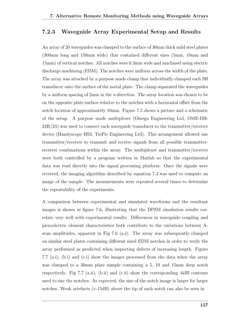
7. Alternative Remote Monitoring Methods using Waveguide Arrays
7.2.3 Waveguide Array Experimental Setup and Results
An array of 20 waveguides was clamped to the surface of 30mm thick mild steel plates
(300mm long and 150mm wide) that contained different sizes (5mm, 10mm and
15mm) of vertical notches. All notches were 0.3mm wide and machined using electric
discharge machining (EDM). The notches were uniform across the width of the plate.
The array was attached by a purpose made clamp that individually clamped each SH
transducer onto the surface of the metal plate. The clamp separated the waveguides
by a uniform spacing of 2mm in the x-direction. The array location was chosen to be
on the opposite plate surface relative to the notches with a horizontal offset from the
notch location of approximately 10mm. Figure 7.5 shows a picture and a schematic
of the setup. A purpose made multiplexer (Omega Engineering Ltd, OME-DB-
24R/24) was used to connect each waveguide transducer to the transmitter/receiver
device (Handyscope HS3, TiePie Engineering Ltd). This arrangement allowed one
transmitter/receiver to transmit and receive signals from all possible transmitter-
receiver combinations within the array. The multiplexer and transmitter/receiver
were both controlled by a program written in Matlab so that the experimental
data was read directly into the signal processing platform. Once the signals were
received, the imaging algorithm described by equation 7.4 was used to compute an
image of the sample. The measurements were repeated several times to determine
the repeatability of the experiments.
A comparison between experimental and simulated waveforms and the resultant
images is shown in figure 7.6, illustrating that the DPSM simulation results cor-
relate very well with experimental results. Differences in waveguide coupling and
piezoelectric element characteristics both contribute to the variations between A-
scan amplitudes, apparent in Fig 7.6 (a.i). The array was subsequently clamped
on similar steel plates containing different sized EDM notches in order to verify the
array performed as predicted when inspecting defects of increasing length. Figure
7.7 (a.i), (b.i) and (c.i) show the images processed from the data when the array
was clamped to a 30mm plate sample containing a 5, 10 and 15mm deep notch
respectively. Fig 7.7 (a.ii), (b.ii) and (c.ii) show the corresponding -6dB contours
used to size the notches. As expected, the size of the notch image is larger for larger
notches. Weak artefacts (<-15dB) above the tip of each notch can also be seen in
157

7. Alternative Remote Monitoring Methods using Waveguide Arrays
Receiver
Amplifier
Toneburst
generator
Handyscope
ADC
MUX Control
Tx
Rx
PC
Specimen
Notch or crack
High temperature
array (a) (b)
Figure 7.5: (a) Schematic of the SH waveguide array and transmit-receive equipment(b) photo of the prototype waveguide array coupled to a 30mm thick steel plate with a5mm notch
Depth = 4.9mm
x-axis (mm)
y-a
xis
(m
m)
0 10 20-30
-25
-20
-15
-10
-5
0
-20
-15
-10
-5
0
Depth = 5mm
x-axis (mm)
y-a
xis
(m
m)
0 10 20-30
-25
-20
-15
-10
-5
0
-20
-15
-10
-5
0
0 10 20 30 40 500
5
10
15
20
time (s)
waveguid
e n
um
ber
0 10 20 30 40 500
5
10
15
20
time (s)
waveguid
e n
um
ber
ima
ge
am
plit
ud
e (
dB
)
(a.i) (a.ii)
(b.i) (b.ii)
ima
ge
am
plit
ud
e (
dB
)
Figure 7.6: Comparison of experimental and simulated results for a 5mm notch in a30mm thick steel plate, (a.i) experimental pitch-catch signals for transmitting transducernumber 8. (a.ii) Image using experimental data. (b.i) Simulated pitch-catch signals fortransmitting transducer number 8. (b.ii) Image using simulated data.
158

7. Alternative Remote Monitoring Methods using Waveguide Arrays
Depth = 14.4mm
x-axis (mm)
y-a
xis
(m
m)
0 10 20-30
-25
-20
-15
-10
-5
0
-20
-15
-10
-5
0
Depth = 9.4mm
x-axis (mm)
y-a
xis
(m
m)
0 10 20-30
-25
-20
-15
-10
-5
0
-20
-15
-10
-5
0Depth = 5mm
x-axis (mm)
y-a
xis
(m
m)
0 10 20-30
-25
-20
-15
-10
-5
0
-20
-15
-10
-5
0dB dB dB
x-axis (mm)
y-a
xis
(m
m)
0 10 20-30
-25
-20
-15
-10
-5
0
x-axis (mm)
y-a
xis
(m
m)
0 10 20-30
-25
-20
-15
-10
-5
0
x-axis (mm)
y-a
xis
(m
m)
0 10 20-30
-25
-20
-15
-10
-5
0
(a.i) (b.i) (c.i)
(a.ii) (b.ii) (c.ii)
Figure 7.7: Images processed from data acquired when the SH array was clamped to a30mm thick steel plate containing (a.i) a 5mm deep notch, (b.i) a 10mm deep notch, (c.i) a15mm deep notch. (a.ii), (b.ii) and (c.ii) show the corresponding -6dB contour plots. (dBvalues are relative to the maximum values in the image, all notches were 0.3mm wide).
each of the images. They occur at points in the image which have the same prop-
agation distances associated with them as the specular reflections from the crack
face, as calculated by equations 7.2 and 7.3. The relatively large amplitude of these
signals means that the artefacts do not completely cancel out during image averag-
ing over the transmitting transducers. These artefacts also exist in images created
using simulated data; however, because of the absence of noise they are lower in
amplitude (<-22dB).
The repeatability of the size measurements for the 10 and 15mm notches was checked
with and without un-clamping the array between each measurement by taking 10
data sets and calculating the mean and standard deviation. The mean notch size
determined from ten repeat measurements of the sample containing a 10mm notch
was 9.49mm with a standard deviation (σd) of 0.14mm. Similarly ten repeat mea-
159
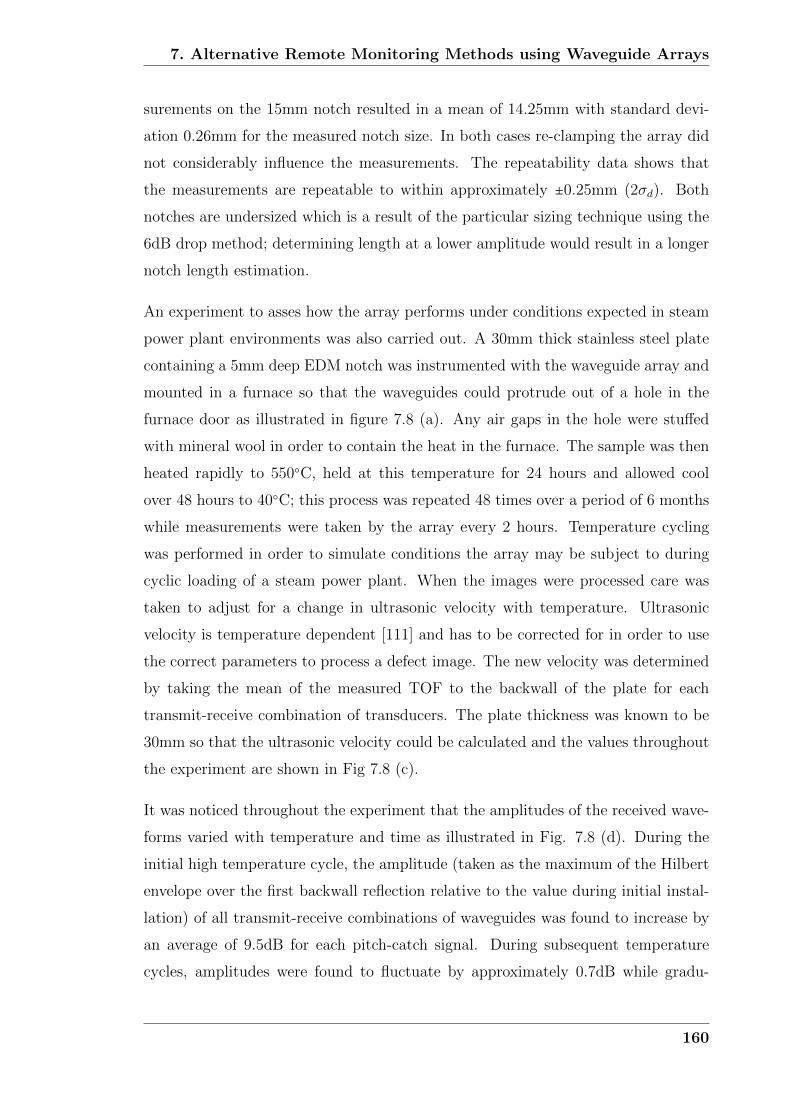
7. Alternative Remote Monitoring Methods using Waveguide Arrays
surements on the 15mm notch resulted in a mean of 14.25mm with standard devi-
ation 0.26mm for the measured notch size. In both cases re-clamping the array did
not considerably influence the measurements. The repeatability data shows that
the measurements are repeatable to within approximately ±0.25mm (2σd). Both
notches are undersized which is a result of the particular sizing technique using the
6dB drop method; determining length at a lower amplitude would result in a longer
notch length estimation.
An experiment to asses how the array performs under conditions expected in steam
power plant environments was also carried out. A 30mm thick stainless steel plate
containing a 5mm deep EDM notch was instrumented with the waveguide array and
mounted in a furnace so that the waveguides could protrude out of a hole in the
furnace door as illustrated in figure 7.8 (a). Any air gaps in the hole were stuffed
with mineral wool in order to contain the heat in the furnace. The sample was then
heated rapidly to 550○C, held at this temperature for 24 hours and allowed cool
over 48 hours to 40○C; this process was repeated 48 times over a period of 6 months
while measurements were taken by the array every 2 hours. Temperature cycling
was performed in order to simulate conditions the array may be subject to during
cyclic loading of a steam power plant. When the images were processed care was
taken to adjust for a change in ultrasonic velocity with temperature. Ultrasonic
velocity is temperature dependent [111] and has to be corrected for in order to use
the correct parameters to process a defect image. The new velocity was determined
by taking the mean of the measured TOF to the backwall of the plate for each
transmit-receive combination of transducers. The plate thickness was known to be
30mm so that the ultrasonic velocity could be calculated and the values throughout
the experiment are shown in Fig 7.8 (c).
It was noticed throughout the experiment that the amplitudes of the received wave-
forms varied with temperature and time as illustrated in Fig. 7.8 (d). During the
initial high temperature cycle, the amplitude (taken as the maximum of the Hilbert
envelope over the first backwall reflection relative to the value during initial instal-
lation) of all transmit-receive combinations of waveguides was found to increase by
an average of 9.5dB for each pitch-catch signal. During subsequent temperature
cycles, amplitudes were found to fluctuate by approximately 0.7dB while gradu-
160

7. Alternative Remote Monitoring Methods using Waveguide Arrays
Dec Jan Feb Mar Apr May Jun Jul2900
3000
3100
3200
3300
3400
time (month)
estim
ate
d w
ave
sp
ee
d (
m/s
)
Dec Jan Feb Mar Apr May Jun Jul
0
5
10
15
20
time (month)
ave
rag
e a
mp
litu
de
ch
an
ge
(d
B)
Dec Jan Feb Mar Apr May Jun Jul5
5.2
5.4
5.6
5.8
6
time (month)
estim
ate
d n
otc
h le
ng
th (
mm
)
5.2 5.4 5.6 5.80
100
200
300
400
500
600
estimated notch length (mm)
fre
qu
en
cy
(a)
(b)
(c)
(d)
(e)
Figure 7.8: (a) Photograph of the experimental setup showing the array and furnace.(b) Histogram of estimated notch lengths showing distribution throughout experiment.(c) Calculated wavespeed throughout experiment. (d) Average amplitude change of firstbackwall reflection of all pitch-catch signals throughout experiment relative to initial am-plitude. (e) Estimated notch length derived from -6dB contour around defect image.
ally increasing, ending at an average increase of 16.5dB. The likely cause of this
initial improvement in signal quality is thermal cycling; material at the contacts
between the waveguides and the substrate plastically deforms at high temperature
and contact pressure, improving the transduction quality between the contacting
interfaces (see for example [112]). Continued plastic and elastic deformation during
subsequent temperature cycles acts to further improve the contact characteristics.
It can be seen in Fig 7.8 (e) that temperature does cause small fluctuations of ap-
proximately 0.15mm in crack length estimate; this is likely caused by not taking the
increase in plate thickness due to thermal expansion into account, therefore chang-
ing how equation 7.4 calculates the notch image. For stainless steel with a thermal
expansion coefficient of 16x10−6, the approximate plate thickness increase would be
0.25mm. If the relationship between temperature and ultrasonic wavespeed was pre-
161

7. Alternative Remote Monitoring Methods using Waveguide Arrays
cisely known within the component material, as well as the current wall thickness,
this error could be removed; however, a detailed knowledge of these parameters at
any one time is unlikely to be available within a steam power plant environment
where other forms of corrosion or erosion may affect the inner surface of the pipe or
pressure vessel. As such this temperature compensation strategy has been identified
as the most applicable for industrial implementation, providing a repeatability of
±0.15mm (2σd). The overestimation of the mean notch length of being 5.53mm is
caused by the choice of amplitude level at which the notch length is estimated (-
6dB). This is not of primary importance since it is the change in fatigue crack length
and measurement repeatability which would be of greatest concern for monitoring
applications.
7.2.4 Prototype Array Industrial Implementation
Following on from experimental validation of the waveguide array under high tem-
perature cyclic loading conditions, an opportunity became available to install a
prototype array on an operational steam power plant at a location identified as con-
taining a thermal fatigue crack during low temperature inspection. The crack was
identified as a circumferential defect, initiating at the butt weld between two CMV
steel pipes feeding steam from the boiler. The plant itself is a former coal-fired
station which is in the process of being converted to fire biomass. Installation was
carried out over a two day period, the first day was taken up with the installation
itself, taking approximately 4 hours to weld the studs and attach the array, ensur-
ing all waveguides were sufficiently clamped to give good quality signals through
the 70mm wall thickness. The second day was predominantly used for data retrieval
and analysis, as well as supervision while insulation was reinstalled around the ar-
ray. The array was installed axially along the pipe with a 20mm offset from the
estimated location of the crack which was sized using TOFD to be approximately
2-3mm in length over the width of the array. Although this crack length is shorter
than the ideal length for the array to detect, it gives scope for detecting an appre-
ciable amount of growth if it does indeed occur during normal operating conditions.
Data acquisition hardware remained the same as that described in section 7.2.3 for
162

7. Alternative Remote Monitoring Methods using Waveguide Arrays
ima
ge
am
plit
ud
e (
dB
)
(a) (b) Crack Depth = 3.6mm
x-axis (mm)
y-a
xis
(m
m)
20 40-70
-60
-50
-40
-30
-20
-10
0
-20
-15
-10
-5
0
Figure 7.9: (a) Photograph of the final array installation (b) Latest crack image, calcu-lated using data taken in January 2012
this initial prototype installation. Connection ports were installed on an adjoining
walkway, 5 metres away from the array in preparation for operator access during
data retrieval using a portable multiplexer and laptop.
A photograph of the final installation is shown in figure 7.9 (a), alongside the latest
crack image. The crack was calculated to be 3.6mm in length, slightly longer than
initially estimated during installation (2.6mm using the array and 2-3mm using
TOFD) which may be due to crack tip opening at high temperature, which was
estimated to be around 210○C at the time of measurement based on the calculated
ultrasonic wavespeed. It is also clear that two reflectors are present in the image;
the stronger reflector with the longest length is taken as the crack with a length
of 3.6mm, with the lower amplitude reflector possibly being an additional crack or
some other reflection caused by a change in pipe cross-sectional area or material
property changes within the butt weld. A definitive conclusion to the cause of this
lower amplitude reflection is difficult to draw without full knowledge of the true
nature of the defect within the weld, as such the higher amplitude reflector has
been taken as the life-limiting defect which should be monitored for future growth.
Data sets were acquired up until January 2012 when conversion to biomass firing
commenced. The main lessons learnt from this initial industrial implementation are
as follows:
163

7. Alternative Remote Monitoring Methods using Waveguide Arrays
� The array survived initial temperature cycling, providing consistent crack size
estimations over a period of 4 months. It is expected that it will still be in
working order once the first data set is taken following plant conversion to
biomass firing.
� Array installation was straight forward using standard drawn-arc stud welding
equipment, requiring minimum surface preparation using an angle grinder.
� It is advised that future installations include an independent temperature mea-
surement of the test structure using a thermocouple in order to verify velocity
calculations and measure the exact temperature conditions the array has been
subjected to.
� Implementation of autonomous or wireless data collection would remove the
need for continued operator access, identified as the limiting factor for more
frequent crack size measurements.
7.3 Velocity Mapping for Detecting Bulk Mate-
rial Degradation
Another application which benefits greatly from the increase in information con-
tent and spatial resolution offered by the array of waveguides is ultrasonic veloc-
ity distribution reconstruction, aimed at detecting and monitoring changes in bulk
material properties. An example of a material degradation mechanism which can
cause such changes is hydrogen attack which often occurs in petrochemical refinery
environments. This form of corrosion is of particular concern when carbon steel
is subjected to high temperatures (>200○C) and high partial pressures (>690KPa)
when in contact with solute hydrogen (H2) which reacts with iron carbide (Fe3C)
to form methane (CH4). The gaseous methane cannot diffuse externally because
of the large molecule size, therefore micro-voids and fissures are formed within the
material structure, often along grain boundaries compromising structural integrity
and in some cases leading to catastrophic failure [113]. The conventional approach
to avoid such failures has been to use materials which are resistant to this type of
degradation, such as low carbon steels containing carbide-forming alloying elements
164

7. Alternative Remote Monitoring Methods using Waveguide Arrays
such as chromium and molybdenum [10]. The Nelson curves serve as a graphical
representation of long-term refinery experience, providing guidance on which alloys
are most resistant under various operating conditions [10]; however, failures con-
tinue to occur with the curves requiring periodic revision [114]. As such an active
nondestructive technique for monitoring hydrogen attack within vulnerable areas of
a structure would be of great value within the petrochemical industry.
Ultrasonic techniques have previously been applied to the detection of hydrogen
attack; specifically techniques based on attenuation, back-scatter and velocity have
been investigated [115]. Both attenuation and backscatter increase in areas subject
to hydrogen attack because of increased scattering caused by micro-defects, however
because the individual defects are around three orders of magnitude smaller than
the ultrasonic wavelength (∼2-60µm [116]), the effect they have on the material as
a whole is to reduce the apparent ultrasonic velocity. Because of the complexity
of the corroded structures formed during hydrogen attack, as well as alternative
material properties such as inclusions and varying grain structure which can cause
very similar changes to ultrasonic signals, conventional detection techniques using
scanning probes suffer from poor measurement repeatability, often leading to false or
missed calls [117]. This represents the major advantage of using the waveguide array
in this application: it can be installed permanently in a vulnerable area operating at
high temperature, allowing very small changes in the measured ultrasonic signals to
be accurately detected, removing any influence of equipment or operator variance.
Based on the accuracy of cross-correlation when calculating the TOF of pulses in
low roughness conditions (see section 4.3.2) and the uncertainty associated with
measuring pulse backscatter, it was decided that velocity calculation would be used
to reconstruct an image of a localised area of material degradation using the array.
The first task was to develop a monitoring strategy based on the expected data
quality and volume, coupled with potential imaging algorithms. Subsequently an
experimental feasibility study was carried out in order to investigate whether the
array is capable of detecting the velocity changes expected during hydrogen attack
in an experimental setting. This was achieved by introducing a transient heat distri-
bution into a test specimen, mimicking the effect an area of hydrogen attack could
have on the velocity distribution within the material. Much of the work presented
165

7. Alternative Remote Monitoring Methods using Waveguide Arrays
has previously been reported in our paper [118], from which some results in the
following sections have been reproduced.
7.3.1 Material Degradation Monitoring Strategy
During hydrogen attack the wall thickness of a pipe or pressure vessel often shows
no decrease in thickness [10], degradation simply develops within the structure. If
this is the case, it is possible to locate areas of differing velocities by calculating the
TOF of pulses reflected from the backwall at different positions within a waveguide
array. Using 20 waveguides this totals 380 pitch-catch signals from which data can
be extracted about the velocity distribution below the array. Two possible ray paths
which travel though the same point on the backwall are illustrated in figure 7.10,
each providing extra information about the form of the defect through which the
waves are travelling. Taking all transmit-receive combinations into account, multiple
ray paths will intersect each image pixel (depending on the assumed width of the ray
and pixel size) providing enhanced information about the velocity experienced within
the material at that point, leading to an an overdetermined system. The task of
the imaging algorithm is to convert the calculated velocity values for each individual
signal into a graphical representation of defect size and location by reconstructing the
most likely spatial distribution of velocity based on the observed data. The algorithm
must do this while remaining stable and achieving the best possible resolution given
the quality of the measured data.
Many different techniques exist which vie to reconstruct images of scatterers based
on wave projections through or from their structure using TOF tomography. A full
review is outside the scope of this thesis; however, the interested reader is referred to
[119–122]. What follows is a description of two methods which were found to provide
the best reconstruction properties based on the form and expected quality of the
data produced by the array. The main challenge faced was a direct result of the
array geometry as illustrated in Fig. 7.10. Comparatively few projections through
the defect structure are available in this limited view setup, with information content
being preferentially distributed along the horizontal direction because of geometrical
limitations. As such, algorithms which are potentially stable with the minimum
number of projections subject to noise were sought.
166

7. Alternative Remote Monitoring Methods using Waveguide Arrays
backwall
hygrogen attack region
array elements
y
x
Figure 7.10: Schematic of array geometry incident upon an area of hydrogen attackshowing two possible ray paths through the area of degradation.
The first, based on the Kaczmarz algorithm (algebraic reconstruction technique),
was selected because it had the potential of utilizing data contained in all 380 signals
recorded by the array and is very often used when solving overdetermined systems
using an iterative procedure [123]. It became clear however that as noise in the data
increased, errors in reconstruction increased dramatically. Therefore a second algo-
rithm was implemented which circumvents the lack of vertical resolution provided
by the limited view array by assuming a vertical exponential velocity distribution
(assumed distribution method), as could potentially be the case for the diffusion
limited propagation of hydrogen within steel. This algorithm has the advantage of
requiring only 19 signals (one between each neighboring waveguide pair), attaining
much greater stability at the expense of approximating the vertical velocity distri-
bution. Further details about the implementation of each of these algorithms will
not be included within this thesis since it was A. Gajdacsi who undertook the ma-
jority of the work in algorithm development; however, results will still be presented
to illustrate the performance of each technique. The interested reader is referred to
our paper [118] for further details.
7.3.2 Temperature Distribution Model
In order to carry out a feasibility study into whether the array could provide accurate
enough velocity calculations to make image reconstruction possible, without requir-
ing a complex and potentially expensive hydrogen attack rig, an alternative approach
167

7. Alternative Remote Monitoring Methods using Waveguide Arrays
was proposed. Since temperature has a similar effect on ultrasonic wavespeed to hy-
drogen attack, a localised heat source was used to produce a transient temperature
distribution within a test specimen. Reconstructing the instantaneous temperature
distribution using ultrasonic data therefore simulates the scenario of reconstruct-
ing an area of material degradation caused by hydrogen attack. However, before
selecting suitable temperatures to subject the test specimen to it was necessary to
estimate the level of ultrasonic velocity change expected during hydrogen attack.
Based on theory presented by Chatterjee [124], the decrease in shear wave velocity
which might be expected in areas of hydrogen attack was estimated to be linearly
dependent with increasing void fraction, decreasing by approximately 1.5% for a
void fraction of 3%. The void fraction represents the volume of material within
the area of degradation which is replaced by micro-scale voids which are randomly
distributed within the area of degradation. These cause a reduction of the material
shear modulus and hence the shear velocity in the material, replicating the effect
early stages of hydrogen attack would have.
An experiment was carried out using the same array setup as described in section
7.2.3 in order to determine the true temperature-wave speed relationship. The steel
sample was uniformly heated using a hot plate as ultrasonic signals were taken
using the array and temperature measurements taken using a k-type thermocouple.
The velocity at each temperature was calculated as the average from all pitch-
catch signals using the TOF of the first backwall reflections. The results of this
experiment are shown in figure 7.11, illustrating a linear trend over the temperatures
experienced. Furthermore, the results indicate temperature differentials no larger
than 100○C are required to simulate void fractions below 3%. It was therefore
concluded that the controllable temperature range within which the experiment
would be carried out would be consistent with velocity changes experienced during
early onset hydrogen attack.
In order to evaluate the ideal imaging capability of each algorithm, a simple steady-
state two dimensional heat conduction simulation was carried out using theory from
[125]. The ideal values of the TOF for each pulse propagating through this temper-
ature distribution were subsequently extracted by integrating time along each ray
path, avoiding any requirement for a more complicated wave propagation simula-
168

7. Alternative Remote Monitoring Methods using Waveguide Arrays
20 30 40 50 60 70 80 90 100 110 1203190
3200
3210
3220
3230
3240
3250
temperature (oC)
ultra
so
nic
wa
ve
sp
ee
d (
m/s
)
experimental data
linear fit
Figure 7.11: Relationship between ultrasonic shear wave velocity and temperature ofmild steel test specimen.
tion using a technique such as FEM since ultrasonic wave refraction was found to
be negligible. These TOF values could then be supplied to the imaging algorithms
to ascertain the capabilities of each in an ideal situation, the results of which are
shown in figure 7.12. It can be seen that in the absence of noise, both algorithms
are able to produce a reconstruction of the true temperature distribution, correctly
locating the hot spot. However, the lack of information available about the distribu-
tion in the vertical direction within the projection data has caused the final solution
provided by the Kaczmarz algorithm to preferentially calculate higher temperatures
closer to the array than they actually occur. This has a knock on effect of reduc-
ing the accuracy of the distribution in the horizontal direction, underestimating the
temperature at the hot spot by 20○C. The assumed distribution technique avoids
this limitation by assuming a vertical distribution, providing a hot spot tempera-
ture estimate within 3○C of the true value, as well as a more accurate temperature
distribution estimate along the full length of the array.
169
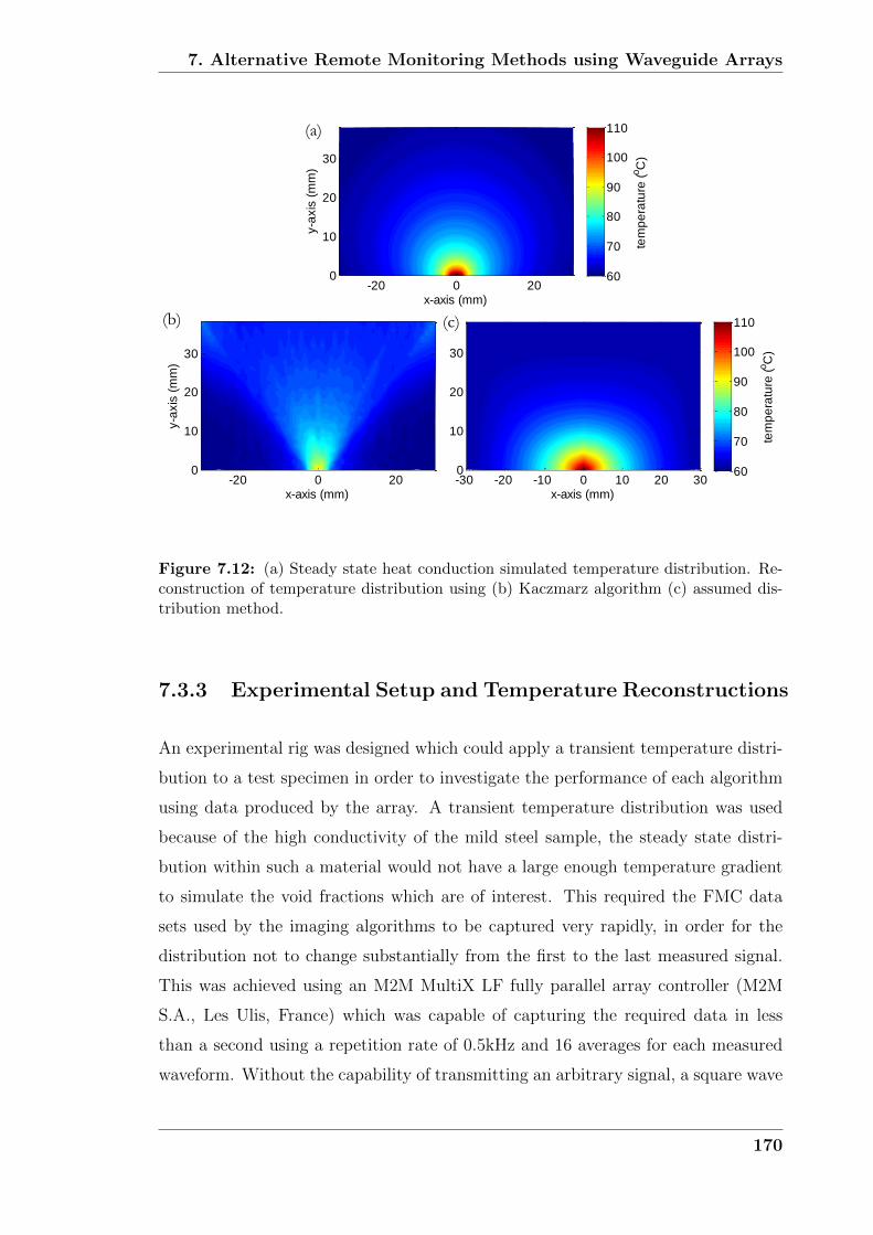
7. Alternative Remote Monitoring Methods using Waveguide Arrays
x-axis (mm)
y-a
xis
(m
m)
-20 0 200
10
20
30
Te
mp
era
ture
(oC
)
60
70
80
90
100
110
x-axis (mm)
y-a
xis
(m
m)
-30 -20 -10 0 10 20 300
10
20
30
tem
pe
ratu
re (
oC
)
60
70
80
90
100
110
(a)
(b) (c)
x-axis (mm)y-a
xis
(m
m)
-20 0 200
10
20
30
tem
pe
ratu
re (
oC
)
60
70
80
90
100
110
Figure 7.12: (a) Steady state heat conduction simulated temperature distribution. Re-construction of temperature distribution using (b) Kaczmarz algorithm (c) assumed dis-tribution method.
7.3.3 Experimental Setup and Temperature Reconstructions
An experimental rig was designed which could apply a transient temperature distri-
bution to a test specimen in order to investigate the performance of each algorithm
using data produced by the array. A transient temperature distribution was used
because of the high conductivity of the mild steel sample, the steady state distri-
bution within such a material would not have a large enough temperature gradient
to simulate the void fractions which are of interest. This required the FMC data
sets used by the imaging algorithms to be captured very rapidly, in order for the
distribution not to change substantially from the first to the last measured signal.
This was achieved using an M2M MultiX LF fully parallel array controller (M2M
S.A., Les Ulis, France) which was capable of capturing the required data in less
than a second using a repetition rate of 0.5kHz and 16 averages for each measured
waveform. Without the capability of transmitting an arbitrary signal, a square wave
170

7. Alternative Remote Monitoring Methods using Waveguide Arrays
was defined using the in-built function generator with a centre frequency of 2MHz,
producing good quality signals ready for processing using cross-correlation (more
details of which can be found in [118]).
In order to create a localised temperature distribution which was approximately
constant along the width of the array, a 500W cylindrical cartridge heater (Fast
Heat Ltd., Eastborne, UK) with a length of 100mm and a diameter of 9.5mm was
used to act as a line source for heat to conduct into the test specimen. A schematic
of the experimental setup is shown in figure 7.13, alongside a photograph of the
final rig. Five k-type thermocouples were attached to the outside surface of the test
specimen in order to assess the form of the temperature distribution, although it is
expected to differ slightly from the distribution within the test specimen at the array
location because of edge convection and a slightly non-uniform heat distribution
along the length of the heating element. Once clamped to the test specimen using
springs to allow for thermal expansion, the heating element was insulated to ensure
maximum heat transfer efficiency at the contact patch. The heating element was
powered using an Elektro-Automatik PS 8000 DT power supply (Viersen, Germany)
set to provide 400W as 60 FMC data sets were taken over a 10 minute period using
the array controller, as well as temperature measurements using a Pico Technology
USB TC-08 thermocouple data logger (Eaton Socon, UK). The pitch between the
waveguides was increased to 3mm to provide a larger array aperture, increasing the
potential area of inspection for the same investment in hardware.
Reconstructions of the temperature distributions provided by Kaczmarz algorithm
and the assumed distribution method using data measured when the hot spot was
at its highest temperature as measured by the thermocouple (115○C) are shown in
figure 7.14. Also shown are the reconstructed temperature distributions calculated at
the same hot spot temperature when the heating element was offset from the centre
for the array by 10mm, demonstrating the positional capabilities of each algorithm.
It can be seen in each case that the general location of the hot spot is correctly
identified; however, Kaczmarz algorithm is much more susceptible to noise within
the calculated velocity data, which is evident from the poor temperature resolution
within the final images. This equates to a hot spot accuracy of approximately
±30○C which was found to be independent of the actual hot spot temperature. In
171
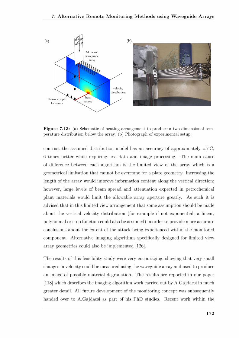
7. Alternative Remote Monitoring Methods using Waveguide Arrays
(a) (b)
thermocouple
locations
heat
source
SH wave
waveguide
array
velocity
distribution
Figure 7.13: (a) Schematic of heating arrangement to produce a two dimensional tem-perature distribution below the array. (b) Photograph of experimental setup.
contrast the assumed distribution model has an accuracy of approximately ±5○C,
6 times better while requiring less data and image processing. The main cause
of difference between each algorithm is the limited view of the array which is a
geometrical limitation that cannot be overcome for a plate geometry. Increasing the
length of the array would improve information content along the vertical direction;
however, large levels of beam spread and attenuation expected in petrochemical
plant materials would limit the allowable array aperture greatly. As such it is
advised that in this limited view arrangement that some assumption should be made
about the vertical velocity distribution (for example if not exponential, a linear,
polynomial or step function could also be assumed) in order to provide more accurate
conclusions about the extent of the attack being experienced within the monitored
component. Alternative imaging algorithms specifically designed for limited view
array geometries could also be implemented [126].
The results of this feasibility study were very encouraging, showing that very small
changes in velocity could be measured using the waveguide array and used to produce
an image of possible material degradation. The results are reported in our paper
[118] which describes the imaging algorithm work carried out by A.Gajdacsi in much
greater detail. All future development of the monitoring concept was subsequently
handed over to A.Gajdacsi as part of his PhD studies. Recent work within the
172
7. Alternative Remote Monitoring Methods using Waveguide Arrays
x-axis (mm)
y-a
xis
(m
m)
-20 0 200
10
20
30
tem
pe
ratu
re (
oC
)
60
80
100
x-axis (mm)
y-a
xis
(m
m)
-20 0 200
10
20
30
tem
pe
ratu
re (
oC
)
60
80
100
x-axis (mm)
y-a
xis
(m
m)
-20 0 200
10
20
30
tem
pe
ratu
re (
oC
)
60
80
100
(a.i) (b.i)
(a.ii) (b.ii)
x-axis (mm)
y-a
xis
(m
m)
-20 0 200
10
20
30
tem
pe
ratu
re (
oC
)
60
80
100
Figure 7.14: Reconstructions of temperature distribution at the end of the experimentusing (a) Kaczmarz algorithm and (b) the assumed distribution method for (i) centralisedheat source and (ii) 10mm offset heat source. The array is located along the top of theimages.
project has focussed on the implementation of an experimental corrosion rig to
simulate real hydrogen attack conditions more accurately, as well as more accurate
signal processing techniques and temperature compensation.
7.4 Summary
Two different applications of an array of waveguide transducers have been investi-
gated and experimentally verified, illustrating the benefits that increased levels of
information can provide when monitoring different forms of corrosion within high
temperature environments. The first of these applications was monitoring circum-
ferential thermal fatigue crack growth at the weld between two sections of piping,
caused by load cycling of a steam power plant. By using the TFM on ultrasonic sig-
nals which had reflected from the crack face via the backwall, it was shown that an
image of a fatigue crack could be produced, from which its location and length could
173

7. Alternative Remote Monitoring Methods using Waveguide Arrays
be estimated and monitored for growth. A simulated study was carried out using
the DPSM to assess the working envelope of the array. The main conclusions were
that a minimum of 15 waveguide transducers would be necessary for measurement
error to be within ±0.25mm and that the defect should be placed in close proximity
to one end of the array, ensuring some offset exists so that backwall reflections do
not encroach upon the defect image. An array of 20 waveguide transducers was
specified for experimental investigations in order to design in some redundancy if
individual transducers fail.
Temperature cycling of a test specimen containing a 5mm long EDM notch was
carried out from 40○C to 550○C, 48 times over a 6 month period, producing a mea-
surement repeatability of ±0.15mm (2σd). The success of this experiment lead to
an opportunity to install a prototype array on an operational coal fired power plant
which has subsequently been converted to biomass firing. Installation was straight
forward and good quality signals were achieved, producing an image of a defect in
the expected location with an initial length estimate of 2.6mm which was within
the 2-3mm estimate provided by an external contractor using conventional TOFD
inspection. Upon temperature cycling this length increased to 3.6mm, possibly
caused by crack tip opening at high temperature. This estimate remained stable for
4 months until the plant was shut down in preparation for conversion to biomass
firing. It is hoped that the success of this initial industrial implementation of the
technology will pave the way for future development, particularly in the area of data
extraction since operator access is limited while the plant is under load.
The second application which has been investigated is monitoring bulk material
degradation caused by hydrogen attack within high temperature, high pressure
petrochemical refinery environments. Micro-voids caused by trapped methane alter
the shear modulus of the material, causing ultrasonic wavespeed to decrease. An
experimental proof of concept study was carried out to asses whether the signals
produced by the waveguide array using existing signal processing techniques would
be sensitive enough to the small velocity differentials expected under early onset
hydrogen attack. To simulate these conditions experimentally a two dimensional
temperature distribution was applied to the test specimen using a cylindrical car-
tidge heater, producing SH wave velocity distributions which would be equivalent
174

7. Alternative Remote Monitoring Methods using Waveguide Arrays
to void fractions within hydrogen attacked regions of up to 3%.
Two TOF tomography imaging algorithms were selected as the most applicable
within the high noise, limited view geometry offered by the array: the Kaczmarz
algorithm and the assumed distribution technique. Both were found to successfully
locate the hot spot within the experimental data; however the lack of information
within the projections related to the vertical velocity distribution caused the Kacz-
marz algorithm to underestimate the temperature of the hot spot by approximately
30○C. Noise in the data also greatly affected the images produced by the algorithm.
The assumed distribution method circumvented this lack of vertical information by
assuming an exponential form to the temperature below the array, producing hot
spot temperature estimates to within 5○C of that indicated by thermocouple mea-
surements. However, the simplicity of the assumed distribution technique requires
an approximation to be made and only 5% of the information held in the FMC
data set is exploited. Further work should be carried out investigating alternative
imaging algorithms for use in limited view geometries, as well as better simulation
of the actual hydrogen attack environment. The success of this experiment at de-
tecting very small changes in ultrasonic velocity indicates that a robust monitoring
technique could be developed using the waveguide array; however, further study is
outside the scope of this thesis and future work will be carried out by A.Gajdacsi.
The two practical applications of a high temperature waveguide array presented
in this chapter show promise for future structural degradation monitoring within
extreme environments, however they are not the only opportunities provided by
the technology. It is hoped that the work presented in this chapter will provide a
footing for others to expand upon and develop solutions to a wider range of non-
destructive corrosion monitoring problems encountered within various challenging
operating conditions.
175

Chapter 8
Conclusions
8.1 Thesis review
A new approach to simulating ultrasonic wave scattering from rough surfaces has
been presented in this thesis, developed using the semi-analytical mesh-free DPSM.
A reduction in simulation time of around three orders of magnitude over the FEM is
a clear indication of the improvement in efficiency over meshed numerical techniques.
The inclusion of multiple scattering, surface self-shadowing and edge diffraction also
improve accuracy over approximate analytical techniques such as classical Kirchhoff
theory. The ability to define arbitrary incidence fields, as well as calculate field
variables within the near-field are also great advantages offered by the technique.
The results from the simulation were subsequently used to improve the quantitative
analysis of ultrasonic signals gathered during wall thickness monitoring of corroding
components within high temperature environments.
Chapter 2 outlined the challenges still faced when modelling ultrasound scattering
from rough surfaces. It began by presenting the equations which must be solved
when simulating mechanical wave propagation within solid structures, introduc-
ing the powerful simplification that the scalar wave approximation can bring when
considering SH wave propagation in two dimensional geometries. A description of
current techniques concluded that although many exist, few strike a good balance
between simulation complexity, efficiency and accuracy. Chapter 3 then introduced
176

8. Conclusions
the DPSM as an alternative which was comparatively simple to implement, required
equations to be solved only along problem boundaries and inherently included mul-
tiple scattering, surface self-shadowing and edge diffraction within the boundary
integral matrix equation. Results produced by the DPSM were indistinguishable
from those produced using the FEM, and further validation against experimental
results gained using the waveguide transducers also indicated that the scalar wave
approximation was sufficient to capture SH wave scattering behaviour in two dimen-
sional geometries.
Chapter 4 then focussed on using the simulation to assess TOF algorithm stability for
wall thickness monitoring within corroded environments using rough surfaces with
Gaussian distributed height and length characteristics. It was found that roughness
can have a large impact on reflected pulse shape, and TOF algorithms based on
earliest signal arrival are most stable under high roughness conditions (σ > 0.1λ).
Signal quality metrics were also proposed as probabilistic measures of the error in
thickness measurement based on the shape change of the pulse. Correlation coeffi-
cient showed the most promise; however, it was clear that insufficient information
is carried within a single reflected pulse to determine characteristics of the surface
itself.
The efficiency of the DPSM was then exploited fully by applying it to scattering in
three dimensions from comparatively large (10x17λ) and rough reflectors in Chap-
ter 5. Efficiency enhancing techniques such as GMRes, beam superposition and
parallel processing all combined to produce a simulation time of approximately 30
minutes, which is currently impossible to achieve using the FEM with comparable
simulation objectives and computing power. Validation could only be carried out
by comparison to experimental results, showing agreement in both amplitude and
pulse shape within expected experimental error bounds even when using the scalar
wave approximation. Furthermore, having access to simulated results from both two
dimensional and three dimensional rough surface geometries allowed direct compari-
son, leading to the proposal of a correction procedure which could be used to convert
results gained rapidly in two dimensions to more closely resemble those from rough
surfaces in three dimensions.
Alternative corroded surface geometries were considered in Chapter 6, focussing on
177
8. Conclusions
localised pitting. Experimental results illustrated the extremes which could be ex-
pected for signal change from singular defects over micron and millimetre length
scales. Comparison to experimental results using a surface taken from a real cor-
roded sample again showed the simulation capable of predicting signal shape change
under increasingly corroded conditions. A corrosion model was subsequently taken
from literature and used alongside the DPSM to describe how defect morphology
through time can change ultrasonic signal shape and corrosion rate predictions using
different TOF algorithms.
Monitoring of structural degradation mechanisms other than wall thickness loss was
explored in Chapter 7 using array geometries to increase data availability. Two
applications were considered: thermal fatigue crack monitoring and bulk material
degradation through hydrogen attack. Both were shown to be possible using an
array architecture and the current waveguide transducer; it is hoped that similar
application of the technology could provide monitoring solutions for other defect
morphologies within high temperature environments.
8.2 Main findings
Accurate simulation of how waves interact with rough boundaries during reflection
is a very complex problem to solve. Applications involving such interactions span
many scientific and engineering disciplines making it the focal point of much litera-
ture. This importance and complexity has lead to many different techniques being
proposed with associated strengths and weaknesses. The main aim of the work pre-
sented in this thesis was to present an alternative which maximised efficiency with a
minimum impact on the accuracy of the final simulated result; the practical applica-
tion being the NDE of wall thickness using permanently installed ultrasonic sensors
within high temperature and corrosive environments. This was achieved by devel-
oping a simulation based on the DPSM, a semi-analytical mesh-free BIE technique
which previously had not been applied to the problem of rough surface scattering.
It allowed simulations to be carried out within the near field of comparatively large
reflectors, including effects such as multiple scattering and surface self-shadowing,
within timescales appropriate for statistical analysis investigations to be performed.
178

8. Conclusions
The alteration to standard DPSM for application to purely two dimensional geome-
tries was described in detail (as published in [P5]), as well as comparison of the three
dimensional model to experimental results (to be published in [P6]). Its simplicity,
efficiency and accuracy make it a strong candidate for future use by researchers
investigating wave scattering, from electromagnetic waves to ultrasonic waves.
The scalar wave approximation has been utilised throughout this thesis as a simpli-
fying assumption which is mathematically only valid for SH wave scattering in two
dimensional geometries. It was shown by comparison to experimental results that
this was indeed the case; however, for the surface geometries and waveguide trans-
ducers considered, it was also found that the amplitude and pulse shape changes
predicted using the scalar wave model in three dimensions agreed within the exper-
imental error bounds of the SH wave transducers. Therefore, the extra complexity
associated with a full elastodynamic analysis of SH wave scattering in three dimen-
sions was shown to be unnecessary since the majority of the physical interactions are
captured using much simpler scalar waves. The experimental results of scattering
from a three dimensional rough surface also served to illustrate the large variability
that can exist in scattered response when a sensor is installed at different locations
separated by only 1.25λ (to be published in [P6]).
Analysis of signals produced using the simulation was carried out in order to assess
the levels of roughness beyond which various TOF algorithms became unstable. It
was found that cross-correlation is superior to envelope peak detection and threshold
first arrival in accurately determining wall thickness when σ < 0.1λ; however, as
roughness increases and diffuse energy acts to completely distort the shape of the
scattered pulse, algorithms based on finding the earliest arrival of the pulse become
the most stable. The performance of such algorithms is directly linked to how low
the detection threshold can be set, potentially limiting their application in field
results (as published in [P2] and [P5]). The limited data available within a single
reflected pulse was also shown to be insufficient for deterministic conclusions to be
drawn about the nature of the surface causing the shape change. The correlation
coefficient could potentially be used to estimate thickness measurement uncertainty;
however, direct application to field results would be challenging.
Another novel investigation which was carried out in this thesis thanks to the simu-
179

8. Conclusions
lation developed was the comparison between results gained using both two dimen-
sional and three dimensional geometries. It was found that although coherent energy
within the scattered pulses was similar for comparable RMS height and correlation
length parameters, diffuse energy dominated two dimensional results because of a
lack of out-of-plane spatial averaging. This means that for given surface statistics,
two dimensional results should always be considered as a worst case scenario. It
was found that the reduction in the RMS height of the average surface beneath
the sensor contact patch could be used directly to reduce the diffuse energy compo-
nent within two dimensional results to produce simulated results which much more
closely approximated what would be expected in three dimensions. The correction
procedure was found to work well when λ0 ≤ λ and σ < λ/5 for sensor widths greater
than 2.5λ and less than 7.5λ.
The extra information available in an array geometry allowed the waveguide trans-
ducer to be applied to other high temperature NDE monitoring applications. The
TFM was applied to thermal fatigue crack monitoring and shown experimentally to
produce repeatable and accurate measurements of EDM notches during sustained
temperature cycling over a 6 month period (as published in [P1] and [P3]). A pro-
totype was subsequently installed on an operational power plant and shown capable
of producing stable estimates of crack length and position, the first such implemen-
tation in the world. A method of monitoring hydrogen attack by reconstructing
ultrasonic velocity using backwall reflections in the limited view array geometry was
also presented. An experimental feasibility study, carried out using a transient two
dimensional temperature distribution to simulate the effect localised hydrogen at-
tack could have, indicated that the levels of velocity change expected during such
degradation could be measured using the current transducers (to be published in
[P7]). Temperature distribution reconstructions carried out using two different al-
gorithms (Kaczmarz algorithm and the assumed distribution technique) successfully
detected the location and approximate temperature of the hot spot; however, fur-
ther work is necessary to utilise all the data available within the limited view FMC
data set.
180

8. Conclusions
8.3 Areas for future work
Although experimental results presented in this thesis suggest the scalar wave ap-
proximation is sufficient for modelling SH wave scattering from the rough sur-
faces considered using the waveguide transducer geometry described, to the au-
thors knowledge no simulation technique exists which is capable of modelling elastic
wave scattering from large rough three dimensional reflectors within the near field.
This makes formal comparison of simulated elastic and scalar wave results impos-
sible. The validity of the scalar wave approximation when modelling elastic wave
scattering from surfaces with increasing levels of roughness and alternative defect
morphologies will therefore remain uncertain. To address this issue, one future av-
enue of research could be the development of a simulation technique which is capable
of efficiently and accurately simulating elastic wave scattering at rough boundaries.
Based on the success of the scalar wave DPSM, the obvious choice would be use
its elastodynamic form as described in Chapter 4 of [51]; however, the results from
an initial implementation carried out using Matlab indicate a potential problem as
illustrated in figure 8.1.
The simple scenario of a point load within an infinite solid medium under plane
strain conditions was chosen to verify results given by the elastic DPSM were the
same as the FEM before the simulation was developed any further. It was found
that in the near field there was a large difference between calculated displacements
produced by the elastic DPSM and the FEM as illustrated in Fig. 8.1 (b) which
becomes negligible for propagation distances greater than approximately 3.7mm
(2.3λ). Accuracy of the equations within the near field is imperative for the final
scattered field to remain correct since point sources must be placed in close proximity
to the boundaries. Since a reason for this discrepancy was not forthcoming and
because it was not necessary for the results presented within this thesis, further
development was halted. However, future work could pick up where this simulation
left off and improve upon the near field behaviour of the elastic DPSM.
Of the TOF algorithms investigated in Chapter 4 of this thesis, cross-correlation was
found to provide the most accurate wall thickness estimates when RMS height was
low (σ < 0.1λ), and threshold first arrival was the most stable over the full range of
181

8. Conclusions
x1
x2 Observation line
r
θ=45°
Point load = 0.1N
Infinite steel medium (plane strain)
0 2 4 6-0.1
-0.05
0
0.05
0.1
time (s)
dis
pla
ce
me
nt (p
m)
x1=0.75mm, x
2=0.75mm, r=1.0607mm
u1 DPSM
u2 DPSM
u1 FEM
u2 FEM
0 2 4 6-0.1
-0.05
0
0.05
0.1
time (s)d
isp
lace
me
nt (p
m)
x1=2.6mm, x
2=2.6mm, r=3.677mm
(a)
(b) (c) (d)
0 2 4 6-0.1
-0.05
0
0.05
0.1
time (s)
dis
pla
ce
me
nt (p
m)
x1=1.65mm, x
2=1.65mm, r=2.3335mm
Figure 8.1: (a) Schematic of simple simulated case. Simulated signals showing horizontaldisplacement (u1) and vertical displacement (u2) produced by the elastic DPSM simula-tion and the two dimensional plane strain FEM simulation using a 2MHz input Hanningwindowed toneburst point load at an observation point where (b) x1 = x2 =0.75mm, (b)x1 = x2 =1.65mm and (c) x1 = x2 =2.60mm.
surface roughnesses considered. The correlation coefficient was also shown to be the
most promising error metric when trying to ascertain a probabilistic measure of the
uncertainty in thickness measurement based on the shape of the reflected pulse. Fol-
lowing on from these simulated studies, the algorithms described should be applied
to field results in order to improve confidence in the corrosion rate estimates, and
to determine whether thickness measurement uncertainty estimation is a possibility
when dealing with real signals. There is also scope for alternate TOF algorithm
development, aimed at combining the strengths of cross-correlation and threshold
first arrival to produce a single algorithm possessing the best possible accuracy over
all roughness levels.
A correction procedure was proposed in Chapter 5 of this thesis which could cor-
rect the high levels of diffuse energy in two dimensional simulations to levels which
182

8. Conclusions
would be more likely in reality based on the characteristics of the scattering surface
and transducer geometry. This concept is potentially very powerful in that it can
reduce the time required for simulated investigations which would otherwise need
to be carried out in three dimensions by several orders of magnitude. Currently it
has only been applied to rough surfaces with Gaussian distributed height and length
characteristics using rectangular strip-like transducer contact patches. Future work
could be carried out to apply the diffuse enrgy correction concept to alternative sce-
narios; for example piston or square transducer geometries, rough surfaces described
by other statistics or even to other wave scattering problems such as grain boundary
scattering in highly attenuative materials.
As described in Chapter 7, further development work has already been undertaken
to improve on the performance of the waveguide array designed to monitor bulk
material degradation such as hydrogen attack in high temperature environments.
Work is still ongoing on designing an electrochemical corrosion rig to simulate more
realistic corrosion environments, as well as the development of more accurate signal
processing techniques to isolate the signal changes caused by hydrogen attack from
those caused by temperature change or thickness loss. The thermal fatigue crack
monitoring array is also currently the subject of further experimental investigations
to see whether the growth of an actual fatigue crack can be measured using a high
temperature fatigue rig. Continued analysis of data from the prototype array on an
operational steam power plant will also provide further proof that the waveguide
array operates consistently within industrial environments and is a candidate for
future commercial development.
183

Appendix
Wall Thickness Box Plots
9
10
11
12
13
0.0
12
0.0
25
0.0
38
0.0
50
0.0
63
0.0
75
0.0
88
0.1
00
0.1
12
0.1
25
0.1
37
0.1
50
0.1
62
0.1
75
0.1
87
RMS height (/c)
estim
ate
d th
ickn
ess (
mm
)
Threshold First Arrival -6dB, 0 = /4
9
10
11
12
13
0.0
12
0.0
25
0.0
38
0.0
50
0.0
63
0.0
75
0.0
88
0.1
00
0.1
12
0.1
25
0.1
37
0.1
50
0.1
62
0.1
75
0.1
87
RMS height (/c)
estim
ate
d th
ickn
ess (
mm
)
Threshold First Arrival -15dB, 0 = /4
9
10
11
12
13
0.0
12
0.0
25
0.0
38
0.0
50
0.0
63
0.0
75
0.0
88
0.1
00
0.1
12
0.1
25
0.1
37
0.1
50
0.1
62
0.1
75
0.1
87
RMS height (/c)
estim
ate
d th
ickn
ess (
mm
)
Cross-correlation, 0 = /4
9
10
11
12
13
0.0
12
0.0
25
0.0
38
0.0
50
0.0
63
0.0
75
0.0
88
0.1
00
0.1
12
0.1
25
0.1
37
0.1
50
0.1
62
0.1
75
0.1
87
RMS height (/c)
estim
ate
d th
ickn
ess (
mm
)
Envelope Peak Detection, 0 = /4(a)
(c)
(b)
(d)
Figure 8.2: Box plots showing the statistical distribution of estimated wall thicknessvalues obtained using the two dimensional DPSM simulation for a 10mm thick wall withRMS heights approaching 0.3mm (σ < λ/5) and a correlation length of 0.4mm (λ0 = λ/4using (a) envelope peak detection (b) cross-correlation (c) threshold first arrival with a-15dB threshold, and (d) threshold first arrival with a -6dB threshold.
184

8. Appendix
9
10
11
12
13
0.0
12
0.0
25
0.0
38
0.0
50
0.0
63
0.0
75
0.0
88
0.1
00
0.1
12
0.1
25
0.1
37
0.1
50
0.1
62
0.1
75
0.1
87
RMS height (/)
estim
ate
d th
ickn
ess (
mm
)
Envelope Peak Detection, 0 = /2
9
10
11
12
13
0.0
12
0.0
25
0.0
38
0.0
50
0.0
63
0.0
75
0.0
88
0.1
00
0.1
12
0.1
25
0.1
37
0.1
50
0.1
62
0.1
75
0.1
87
RMS height (/)
estim
ate
d th
ickn
ess (
mm
)
Threshold First Arrival -15dB, 0 = /2
9
10
11
12
13
0.0
12
0.0
25
0.0
38
0.0
50
0.0
63
0.0
75
0.0
88
0.1
00
0.1
12
0.1
25
0.1
37
0.1
50
0.1
62
0.1
75
0.1
87
RMS height (/)
estim
ate
d th
ickn
ess (
mm
)
Cross-correlation, 0 = /2
9
10
11
12
13
0.0
12
0.0
25
0.0
38
0.0
50
0.0
63
0.0
75
0.0
88
0.1
00
0.1
12
0.1
25
0.1
37
0.1
50
0.1
62
0.1
75
0.1
87
RMS height (/)
estim
ate
d th
ickn
ess (
mm
)
Threshold First Arrival -6dB, 0 = /2
(a)
(c)
(b)
(d)
Figure 8.3: Box plots showing the statistical distribution of estimated wall thicknessvalues obtained using the two dimensional DPSM simulation for a 10mm thick wall withRMS heights approaching 0.3mm (σ < λ/5) and a correlation length of 0.8mm (λ0 = λ/2using (a) envelope peak detection (b) cross-correlation (c) threshold first arrival with a-15dB threshold, and (d) threshold first arrival with a -6dB threshold.
185

8. Appendix
9
10
11
12
13
0.0
12
0.0
25
0.0
38
0.0
50
0.0
63
0.0
75
0.0
88
0.1
00
0.1
12
0.1
25
0.1
37
0.1
50
0.1
62
0.1
75
0.1
87
RMS height (/c)
estim
ate
d th
ickn
ess (
mm
)
Envelope Peak Detection, 0 =
9
10
11
12
13
0.0
12
0.0
25
0.0
38
0.0
50
0.0
63
0.0
75
0.0
88
0.1
00
0.1
12
0.1
25
0.1
37
0.1
50
0.1
62
0.1
75
0.1
87
RMS height (/c)
estim
ate
d th
ickn
ess (
mm
)
Cross-correlation, 0 =
9
10
11
12
13
0.0
12
0.0
25
0.0
38
0.0
50
0.0
63
0.0
75
0.0
88
0.1
00
0.1
12
0.1
25
0.1
37
0.1
50
0.1
62
0.1
75
0.1
87
RMS height (/c)
estim
ate
d th
ickn
ess (
mm
)
Threshold First Arrival -15dB, 0 =
9
10
11
12
13
0.0
12
0.0
25
0.0
38
0.0
50
0.0
63
0.0
75
0.0
88
0.1
00
0.1
12
0.1
25
0.1
37
0.1
50
0.1
62
0.1
75
0.1
87
RMS height (/c)
estim
ate
d th
ickn
ess (
mm
)
Threshold First Arrival -6dB, 0 =
(a)
(c)
(b)
(d)
Figure 8.4: Box plots showing the statistical distribution of estimated wall thicknessvalues obtained using the two dimensional DPSM simulation for a 10mm thick wall withRMS heights approaching 0.3mm (σ < λ/5) and a correlation length of 1.6mm (λ0 = λusing (a) envelope peak detection (b) cross-correlation (c) threshold first arrival with a-15dB threshold, and (d) threshold first arrival with a -6dB threshold.
186

8. Appendix
9
10
11
12
13
0.0
12
0.0
25
0.0
38
0.0
50
0.0
63
0.0
75
0.0
88
0.1
00
0.1
12
0.1
25
0.1
37
0.1
50
0.1
62
0.1
75
0.1
87
RMS height (/c)
estim
ate
d th
ickn
ess (
mm
)
Envelope Peak Detection, 0 = 3/2
9
10
11
12
13
0.0
12
0.0
25
0.0
38
0.0
50
0.0
63
0.0
75
0.0
88
0.1
00
0.1
12
0.1
25
0.1
37
0.1
50
0.1
62
0.1
75
0.1
87
RMS height (/c)
estim
ate
d th
ickn
ess (
mm
)
Cross-correlation, 0 = 3/2
9
10
11
12
13
0.0
12
0.0
25
0.0
38
0.0
50
0.0
63
0.0
75
0.0
88
0.1
00
0.1
12
0.1
25
0.1
37
0.1
50
0.1
62
0.1
75
0.1
87
RMS height (/c)
estim
ate
d th
ickn
ess (
mm
)
Threshold First Arrival -15dB, 0 = 3/2
9
10
11
12
13
0.0
12
0.0
25
0.0
38
0.0
50
0.0
63
0.0
75
0.0
88
0.1
00
0.1
12
0.1
25
0.1
37
0.1
50
0.1
62
0.1
75
0.1
87
RMS height (/c)
estim
ate
d th
ickn
ess (
mm
)
Threshold First Arrival -6dB, 0 = 3/2
(a)
(c)
(b)
(d)
Figure 8.5: Box plots showing the statistical distribution of estimated wall thicknessvalues obtained using the two dimensional DPSM simulation for a 10mm thick wall withRMS heights approaching 0.3mm (σ < λ/5) and a correlation length of 2.4mm (λ0 = 3λ/2using (a) envelope peak detection (b) cross-correlation (c) threshold first arrival with a-15dB threshold, and (d) threshold first arrival with a -6dB threshold.
187
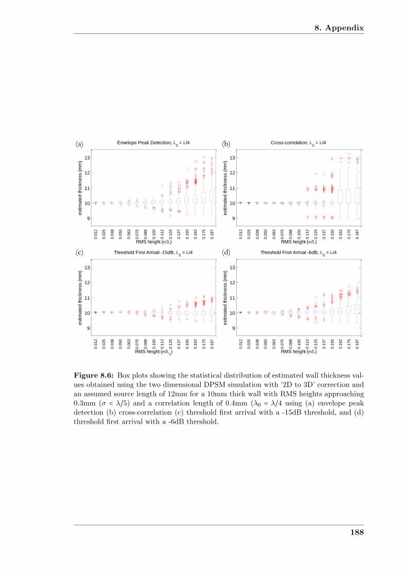
8. Appendix
9
10
11
12
13
0.0
12
0.0
25
0.0
38
0.0
50
0.0
63
0.0
75
0.0
88
0.1
00
0.1
12
0.1
25
0.1
37
0.1
50
0.1
62
0.1
75
0.1
87
RMS height (/)
estim
ate
d th
ickn
ess (
mm
)
Envelope Peak Detection, 0 = /4
9
10
11
12
13
0.0
12
0.0
25
0.0
38
0.0
50
0.0
63
0.0
75
0.0
88
0.1
00
0.1
12
0.1
25
0.1
37
0.1
50
0.1
62
0.1
75
0.1
87
RMS height (/)
estim
ate
d th
ickn
ess (
mm
)
Cross-correlation, 0 = /4
9
10
11
12
13
0.0
12
0.0
25
0.0
38
0.0
50
0.0
63
0.0
75
0.0
88
0.1
00
0.1
12
0.1
25
0.1
37
0.1
50
0.1
62
0.1
75
0.1
87
RMS height (/c)
estim
ate
d th
ickn
ess (
mm
)
Threshold First Arrival -15dB, 0 = /4
9
10
11
12
13
0.0
12
0.0
25
0.0
38
0.0
50
0.0
63
0.0
75
0.0
88
0.1
00
0.1
12
0.1
25
0.1
37
0.1
50
0.1
62
0.1
75
0.1
87
RMS height (/)
estim
ate
d th
ickn
ess (
mm
)
Threshold First Arrival -6dB, 0 = /4
(a)
(c)
(b)
(d)
Figure 8.6: Box plots showing the statistical distribution of estimated wall thickness val-ues obtained using the two dimensional DPSM simulation with ’2D to 3D’ correction andan assumed source length of 12mm for a 10mm thick wall with RMS heights approaching0.3mm (σ < λ/5) and a correlation length of 0.4mm (λ0 = λ/4 using (a) envelope peakdetection (b) cross-correlation (c) threshold first arrival with a -15dB threshold, and (d)threshold first arrival with a -6dB threshold.
188
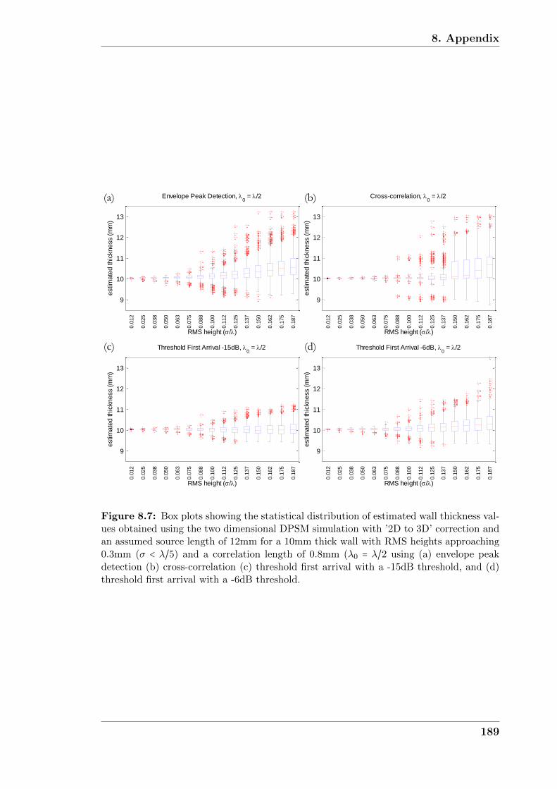
8. Appendix
9
10
11
12
13
0.0
12
0.0
25
0.0
38
0.0
50
0.0
63
0.0
75
0.0
88
0.1
00
0.1
12
0.1
25
0.1
37
0.1
50
0.1
62
0.1
75
0.1
87
RMS height (/)
estim
ate
d th
ickn
ess (
mm
)
Envelope Peak Detection, 0 = /2(a)
(c)
(b)
(d)
9
10
11
12
13
0.0
12
0.0
25
0.0
38
0.0
50
0.0
63
0.0
75
0.0
88
0.1
00
0.1
12
0.1
25
0.1
37
0.1
50
0.1
62
0.1
75
0.1
87
RMS height (/)
estim
ate
d th
ickn
ess (
mm
)
Cross-correlation, 0 = /2
9
10
11
12
13
0.0
12
0.0
25
0.0
38
0.0
50
0.0
63
0.0
75
0.0
88
0.1
00
0.1
12
0.1
25
0.1
37
0.1
50
0.1
62
0.1
75
0.1
87
RMS height (/)
estim
ate
d th
ickn
ess (
mm
)
Threshold First Arrival -15dB, 0 = /2
9
10
11
12
13
0.0
12
0.0
25
0.0
38
0.0
50
0.0
63
0.0
75
0.0
88
0.1
00
0.1
12
0.1
25
0.1
37
0.1
50
0.1
62
0.1
75
0.1
87
RMS height (/)
estim
ate
d th
ickn
ess (
mm
)
Threshold First Arrival -6dB, 0 = /2
Figure 8.7: Box plots showing the statistical distribution of estimated wall thickness val-ues obtained using the two dimensional DPSM simulation with ’2D to 3D’ correction andan assumed source length of 12mm for a 10mm thick wall with RMS heights approaching0.3mm (σ < λ/5) and a correlation length of 0.8mm (λ0 = λ/2 using (a) envelope peakdetection (b) cross-correlation (c) threshold first arrival with a -15dB threshold, and (d)threshold first arrival with a -6dB threshold.
189

8. Appendix
9
10
11
12
13
0.0
12
0.0
25
0.0
38
0.0
50
0.0
63
0.0
75
0.0
88
0.1
00
0.1
12
0.1
25
0.1
37
0.1
50
0.1
62
0.1
75
0.1
87
RMS height (/)
estim
ate
d th
ickn
ess (
mm
)
Envelope Peak Detection, 0 =
9
10
11
12
13
0.0
12
0.0
25
0.0
38
0.0
50
0.0
63
0.0
75
0.0
88
0.1
00
0.1
12
0.1
25
0.1
37
0.1
50
0.1
62
0.1
75
0.1
87
RMS height (/)
estim
ate
d th
ickn
ess (
mm
)
Cross-correlation, 0 =
9
10
11
12
13
0.0
12
0.0
25
0.0
38
0.0
50
0.0
63
0.0
75
0.0
88
0.1
00
0.1
12
0.1
25
0.1
37
0.1
50
0.1
62
0.1
75
0.1
87
RMS height (/)
estim
ate
d th
ickn
ess (
mm
)
Threshold First Arrival -15dB, 0 =
9
10
11
12
13
0.0
12
0.0
25
0.0
38
0.0
50
0.0
63
0.0
75
0.0
88
0.1
00
0.1
12
0.1
25
0.1
37
0.1
50
0.1
62
0.1
75
0.1
87
RMS height (/)
estim
ate
d th
ickn
ess (
mm
)
Threshold First Arrival -6dB, 0 =
(a)
(c)
(b)
(d)
Figure 8.8: Box plots showing the statistical distribution of estimated wall thicknessvalues obtained using the two dimensional DPSM simulation with ’2D to 3D’ correctionand an assumed source length of 12mm for a 10mm thick wall with RMS heights approach-ing 0.3mm (σ < λ/5) and a correlation length of 1.6mm (λ0 = λ using (a) envelope peakdetection (b) cross-correlation (c) threshold first arrival with a -15dB threshold, and (d)threshold first arrival with a -6dB threshold.
190

References
[1] A. Fenster and D.B. Downey. 3-D Ultrasound Imaging : A Review. IEEE
Engineering in Medicine and Biology Magazine, 15(6):41–51, 1996.
[2] S. Kruger, G. Wagner, and D. Eifler. Ultrasonic Welding of Metal/Composite
Joints. Advanced Engineering Materials, 6(3):157–159, 2004.
[3] A.M.K. Thomas, A.K. Banerjee, and U. Busch. Classic Papers in Modern
Diagnostic Radiology. Springer, Berlin, Germany, 2005, pp. 162-170.
[4] F.A. Firestone. The Supersonic Reflectoscope, an Instrument for Inspecting
the Interior of Solid Parts by Means of Sound Waves. The Journal of the
Acoustical Society of America, 17(3):287–299, 1946.
[5] J.D. Achenbach. Quantitative nondestructive evaluation. International Jour-
nal of Solids and Structures, 37:13–27, 2000.
[6] H.C. Furtado and I.L. May. High Temperature Degradation in Power Plants
and Refineries. Materials Research, 7(1):103–110, 2004.
[7] C. Johnston, M.A. Cooper, and R.J. Martin. An Approach to Power Station
Boiler and Turbine Life Management. Insight, 46(10):606–610, 2004.
[8] J. Melville and G. Foster. A pictorial review of failures in conventional boiler
plant. International Journal of Pressure Vessels and Piping, 3(1):1–25, 1975.
[9] I.L. May, T.L. Silveira, and S.K.P. Cheung-Mak. Uncertainties in the evalua-
tion of high temperature damage in power stations and petrochemical plant.
International Journal of Pressure Vessels and Piping, 59:335–343, 1994.
[10] L. Garverick. Corrosion in the Petrochemical Industry. ASM International,
Material Park, OH, 1994, pp. 339-341.
191

REFERENCES
[11] C.J. Moss, P. Barrien, and A. Walczynski. Life management of refinery furnace
tubing. International Journal of Pressure Vessels and Piping, 77:105–112,
2000.
[12] R. Kazys, A. Voleisis, and B. Voleisiene. High temperature ultrasonic trans-
ducers : review. Ultrasound, 63(2):7–17, 2008.
[13] R.E. Green. Non-contact ultrasonic techniques. Ultrasonics, 42(1-9):9–16,
2004.
[14] S. Dixon, C. Edwards, and S.B. Palmer. High accuracy non-contact ultrasonic
thickness gauging of aluminium sheet using electromagnetic acoustic transduc-
ers. Ultrasonics, 39:445–453, 2001.
[15] S.E. Kruger, M. Lord, and J.P. Monchalin. Laser Ultrasonic Thickness Mea-
surements of Very Thick Walls at High Temperatures. volume 25, pages 240–
247, 2006.
[16] W.A. Grandia and C.M. Fortunko. NDE Applications of Air-Coupled Ultra-
sonic Transducers. In IEEE Ultrasonics Symposium, volume 1, pages 697–709,
1995.
[17] K.J. Kirk, A. Mcnab, A. Cochran, I. Hall, and G. Hayward. Ultrasonic Arrays
for Monitoring Cracks in an Industrial Plant at High Temperatures. IEEE
Transactions on Ultrasonics, Ferroelectrics and Frequency Control, 46(2):311–
319, 1999.
[18] A. Mcnab, K.J. Kirk, and A. Cochran. Ultrasonic transducers for high temper-
ature applications. IEEE Proceedings - Science, Measurement and Technology,
145(5):229–236, 1998.
[19] K.J. Kirk, C.K. Lee, S. Cochran, A. McNab, and G. Shepherd. Condition
monitoring with ultrasonic arrays at elevated temperatures. Insight, 45(2):130–
133, 2003.
[20] N. Schmarje, J.F. Saillant, K.J. Kirk, and S. Cochran. Imaging with lithium
niobate/epoxy composites. Ultrasonics, 42:439–442, 2004.
192

REFERENCES
[21] N. Schmarje, K.J. Kirk, and S. Cochran. 1-3 Connectivity Lithium Niobate
Composites for High Temperature Operation. Ultrasonics, 47:15–22, 2007.
[22] S.P. Kelly, I. Atkinson, C. Gregory, and K.J. Kirk. On-Line Ultrasonic Inspec-
tion at Elevated Temperatures. In IEEE Ultrasonics Symposium Proceedings,
pages 904–908. IEEE, 2007.
[23] Y. Liu, L.C. Lynnworth, and M.A. Zimmerman. Buffer waveguides for flow
measurement in hot fluids. Ultrasonics, 36:305–315, 1998.
[24] Y. Ono, C.K. Jen, and M. Kobayashi. High temperature integrated ultra-
sonic shear and longitudinal wave probes. Review of Scientific Instruments,
78(2):024903–1–024901–5, 2007.
[25] M. Kobayashi, C.K. Jen, J.F. Bussiere, and K.T. Wu. High-temperature in-
tegrated and flexible ultrasonic transducers for nondestructive testing. NDT
& E International, 42(2):157–161, 2009.
[26] F.B. Cegla. Energy concentration at the center of large aspect ratio rectangu-
lar waveguides at high frequencies. The Journal of the Acoustical Society of
America, 123(6):4218–4226, 2008.
[27] F.B. Cegla and J.O. Davies. Ultrasonic Crack Monitoring At High Tempera-
tures Using SH Waves (¿500C). volume 29, pages 980–987, 2010.
[28] K. Balasubramaniam, V.V. Shah, R.D. Costley, G. Boudreaux, and J.P.
Singh. High temperature ultrasonic sensor for the simultaneous measure-
ment of viscosity and temperature of melts. Review of Scientific Instruments,
70(12):4618–4623, 1999.
[29] F.B. Cegla. Ultrasonic Waveguide Sensors For Fluid Characterisation And
Remote Sensing. PhD thesis, Imperial College London, 2006.
[30] F.B. Cegla, P. Cawley, J. Allin, and J.O. Davies. High-Temperature (> 500○C)
Wall Thickness Monitoring Using Dry-Coupled Ultrasonic Waveguide Trans-
ducers. IEEE Transactions on Ultrasonics, Ferroelectrics and Frequency Con-
trol, 58(1):156–167, 2011.
193

REFERENCES
[31] A.J.C. Jarvis and F.B. Cegla. Application of the distributed point source
method to rough surface scattering and ultrasonic wall thickness measurement.
Journal of the Acoustical Society of America, 132(3):1325–1335, 2012.
[32] A.J.C. Jarvis and F.B. Cegla. Scattering of SH Waves by Sinusoidal and Rough
Surfaces in 3D: Comparison to the Scalar Wave Approximation. Submitted to.
NDT & E International, 2013.
[33] J.A. Hudson. The Excitation and Propagation of Elastic Waves. Cambridge
University Press, Cambridge, 1980.
[34] J.L. Rose. Ultrasonic Waves in Solid Media. Cambridge University Press,
Cambridge, 1999.
[35] G.S. Kino. Acoustic Waves: Devices, Imaging and Analog Signal Processing.
Prentice-Hall, inc., New Jersey, 1987.
[36] J.L. Uretsky. Reflection of a Plane Sound Wave from a Sinusoidal Surface.
Atomic Energy, 290(1930):1293–1294, 1963.
[37] L. Fortuin. Survey of Literature on Reflection and Scattering of Sound
Waves at the Sea Surface. The Journal of the Acoustical Society of Amer-
ica, 47(5B):1209–1228, 1970.
[38] J.A. Ogilvy. Wave scattering from rough surfaces. Reports on Progress in
Physics, 50:1553–1608, 1987.
[39] T.M. Elfouhaily and C. Guerin. A critical survey of approximate scatter-
ing wave theories from random rough surfaces. Waves in Random Media,
14(4):R1–R40, 2004.
[40] K.F. Warnick and W.C. Chew. Numerical simulation methods for rough sur-
face scattering. Waves in Random Media, 11(1):R1–R30, 2001.
[41] M. Saillard and A. Sentenac. Rigorous solutions for electromagnetic scattering
from rough surfaces. Waves in Random Media, 11(3):R103–R137, 2001.
[42] J.A. Ogilvy. Computer simulation of acoustic wave scattering from rough
surfaces. Physics, 21:260–277, 1988.
194
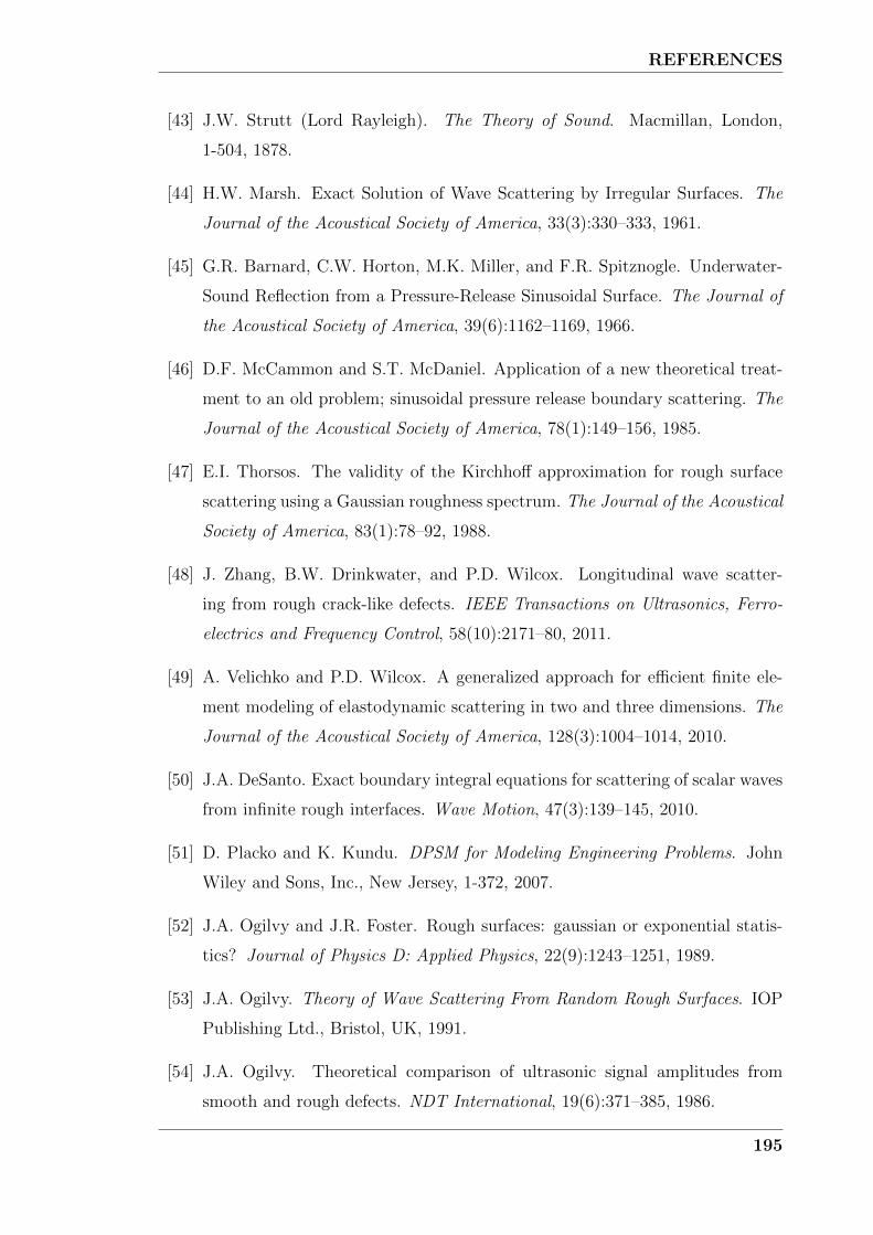
REFERENCES
[43] J.W. Strutt (Lord Rayleigh). The Theory of Sound. Macmillan, London,
1-504, 1878.
[44] H.W. Marsh. Exact Solution of Wave Scattering by Irregular Surfaces. The
Journal of the Acoustical Society of America, 33(3):330–333, 1961.
[45] G.R. Barnard, C.W. Horton, M.K. Miller, and F.R. Spitznogle. Underwater-
Sound Reflection from a Pressure-Release Sinusoidal Surface. The Journal of
the Acoustical Society of America, 39(6):1162–1169, 1966.
[46] D.F. McCammon and S.T. McDaniel. Application of a new theoretical treat-
ment to an old problem; sinusoidal pressure release boundary scattering. The
Journal of the Acoustical Society of America, 78(1):149–156, 1985.
[47] E.I. Thorsos. The validity of the Kirchhoff approximation for rough surface
scattering using a Gaussian roughness spectrum. The Journal of the Acoustical
Society of America, 83(1):78–92, 1988.
[48] J. Zhang, B.W. Drinkwater, and P.D. Wilcox. Longitudinal wave scatter-
ing from rough crack-like defects. IEEE Transactions on Ultrasonics, Ferro-
electrics and Frequency Control, 58(10):2171–80, 2011.
[49] A. Velichko and P.D. Wilcox. A generalized approach for efficient finite ele-
ment modeling of elastodynamic scattering in two and three dimensions. The
Journal of the Acoustical Society of America, 128(3):1004–1014, 2010.
[50] J.A. DeSanto. Exact boundary integral equations for scattering of scalar waves
from infinite rough interfaces. Wave Motion, 47(3):139–145, 2010.
[51] D. Placko and K. Kundu. DPSM for Modeling Engineering Problems. John
Wiley and Sons, Inc., New Jersey, 1-372, 2007.
[52] J.A. Ogilvy and J.R. Foster. Rough surfaces: gaussian or exponential statis-
tics? Journal of Physics D: Applied Physics, 22(9):1243–1251, 1989.
[53] J.A. Ogilvy. Theory of Wave Scattering From Random Rough Surfaces. IOP
Publishing Ltd., Bristol, UK, 1991.
[54] J.A. Ogilvy. Theoretical comparison of ultrasonic signal amplitudes from
smooth and rough defects. NDT International, 19(6):371–385, 1986.
195
REFERENCES
[55] MATLAB Reference Manuals, Version 7.9.0.529. The Mathworks, Inc., Nat-
ick, MA, 2009.
[56] T. Kundu, D. Placko, E. K. Rahani, T. Yanagita, and C. M. Dao. Ultrasonic
Field Modeling : A Comparison Numerical Techniques. IEEE Transactions
on Ultrasonics, Ferroelectrics and Frequency Control, 57(12):2795–2807, 2010.
[57] R. Ahmad, T. Kundu, and D. Placko. Modeling of phased array transducers.
The Journal of the Acoustical Society of America, 117(4):1762, 2005.
[58] S. Banerjee, T. Kundu, and N. Alnuaimi. DPSM technique for ultrasonic field
modelling near fluid-solid interface. Ultrasonics, 46(3):235–50, 2007.
[59] S. Banerjee and T. Kundu. Ultrasonic field modeling in plates immersed in
fluid. International Journal of Solids and Structures, 44(18-19):6013–6029,
2007.
[60] S. Banerjee and T. Kundu. Semi-analytical modeling of ultrasonic fields in
solids with internal anomalies immersed in a fluid. Wave Motion, 45(5):581–
595, 2008.
[61] S. Banerjee and T. Kundu. Elastic wave field computation in multilayered
nonplanar solid structures: a mesh-free semianalytical approach. The Journal
of the Acoustical Society of America, 123(3):1371–82, 2008.
[62] A. Shelke, S. Das, and T. Kundu. Distributed Point Source Method for Mod-
eling Scattered Ultrasonic Fields in Presence of an Elliptical Cavity. Structural
Health Monitoring, 0(0):1–13, 2010.
[63] S. Banerjee, S. Das, T. Kundu, and D. Placko. Controlled Space Radiation
concept for mesh-free semi-analytical technique to model wave fields in com-
plex geometries. Ultrasonics, 49(8):615–22, 2009.
[64] S. Wooh and Y. Shi. Optimum beam steering of linear phased arrays. Wave
Motion, 29(3):245–265, 1999.
[65] T. Yanagita, T. Kundu, and D. Placko. Ultrasonic field modeling by dis-
tributed point source method for different transducer boundary conditions.
The Journal of the Acoustical Society of America, 126(5):2331–9, 2009.
196

REFERENCES
[66] J. Cheng, W. Lin, and Y. Qin. Extension of the distributed point source
method for ultrasonic field modeling. Ultrasonics, 51(5):571–580, 2010.
[67] E.K. Rahani and T. Kundu. Modeling of Transient Ultrasonic Wave Prop-
agation Using the Distributed Point Source Method. IEEE Transactions on
Ultrasonics, Ferroelectrics and Frequency Control, 58(10):2213–2221, 2011.
[68] L.W. Schmerr. Fundamentals of Ultrasonic Nondestructive Evaluation.
Plenum Press, New York, 1998.
[69] R.J. Wombell and J.A. DeSanto. Reconstruction of rough-surface profiles
with the Kirchhoff approximation. Journal of the Optical Society of America
A, 8(12):1892–1897, 1991.
[70] D.R. Melton and C.W. Horton. Importance of the Fresnel Correction in Scat-
tering from a Rough Surface . I . Phase and Amplitude Fluctuations. Journal
of the Acoustical Society of America, 47(1B):290–298, 1970.
[71] N.C. Bruce and J.C. Dainty. Multiple Scattering from Random Rough Surfaces
Using the Kirchhoff Approximation. Journal of Modern Optics, 38(3):579–590,
1991.
[72] P. Beckmann. Shadowing of Random Rough Surfaces. IEEE Transactions on
Antennas and Propagation, 13(3):384–388, 1965.
[73] R.J. Wagner. Shadowing of Randomly Rough Surfaces. The Journal of the
Acoustical Society of America, 41(1):138–147, 1967.
[74] M.V. Berry. On deducing the form of surfaces from their diffracted echoes.
Physics, 5:272–291, 1972.
[75] ABAQUS Reference Manuals, Version 6.9. ABAQUS Inc., Providence, RI,
2010.
[76] E. K. Rahani and T. Kundu. Gaussian-DPSM (G-DPSM) and Element Source
Method (ESM) modifications to DPSM for ultrasonic field modeling. Ultra-
sonics, 51(5):625–631, 2011.
[77] A.J. Croxford, P.D. Wilcox, G. Konstantinidis, and B.W. Drinkwater. Strate-
gies for Overcoming the Effect of Temperature on Guided Wave Structural
197

REFERENCES
Health Monitoring. In Proceedings of the SPIE, volume 6532, page 65321T,
2007.
[78] C. Canali, G. De Cicco, B. Morten, M. Prudenziati, and A. Taroni. A Tem-
perature Compensated Ultrasonic Sensor Operating in Air for Distance and
Proximity Measurements. IEEE Transactions on Industrial Electronics, IE-
29(4):336–341, 1982.
[79] S.W. Smith. The Scientist and Engineer’s Guide to Digital Signal Processing.
California Technical Publishing, San Diego, CA, 1997.
[80] D. Liu and R.C. Waag. Correction of ultrasonic wavefront distortion using
backpropagation and a reference waveform method for time-shift compensa-
tion. The Journal of the Acoustical Society of America, 96(2):649–660, 1994.
[81] J.S. Bendat and A.G. Piersol. Random Data: Analysis and Measurement
Procedures. Wiley, 2010.
[82] DISPERSE User Manual, Version 2.0.16B. Imperial College of Science, Tech-
nology and Medicine, London, London, UK, 2003.
[83] Y. Saad and M.H. Schultz. GMRES: A Generalized Minimal Residual Algo-
rithm for Solving Nonsymmetric Linear Systems. SIAM Journal on Scientific
and Statistical Computing, 7(3):856–869, 1986.
[84] M. Saillard and D. Maystre. Scattering from Random Rough Surface: A Beam
Simulation Method. Journal of Optics, 19(4):173–176, 1988.
[85] C.J.R. Sheppard and T.J. Connolly. Imaging of Random Surfaces. Journal of
Modern Optics, 42(4):861–881, 1995.
[86] J. Kvarekval. Morphology of Localised Corrosion Attacks in Sour Environ-
ments. In Corrosion, number 07659, pages 1–10, 2007.
[87] C. Shargay, K. Moore, and R. Colwell. Survey of Materials in Hydroheater
Units Processing High TAN Feeds. In Corrosion, number 07573, pages 1–11,
2007.
[88] X. Wu, H. Jing, Y. Zheng, Z. Yao, and W. Ke. Erosion-corrosion of various
oil-refining materials in naphthenic acid. Wear, 256(1-2):133–144, 2004.
198

REFERENCES
[89] E. Slavcheva, B. Shone, and A. Turnbull. Factors Contolling Naphthenic Acid
Corrosion. In Corrosion, number 579, pages 1–19, 1998.
[90] D.R. Qu, Y.G. Zheng, H.M. Jing, Z.M. Yao, and W. Ke. High tempera-
ture naphthenic acid corrosion and sulphidic corrosion of Q235 and 5Cr1/2Mo
steels in synthetic refining media. Corrosion Science, 48(8):1960–1985, 2006.
[91] M.J. Zetlmeisl. Naphthenic Acid Corrosion and its Control. In Corrosion,
number 218, pages 1–8, 1996.
[92] R.D. Kane and M.S. Cayard. A Comprehensive Study on Naphthenic Acid
Corrosion. In Corrosion, number 02555, pages 1–16, 2002.
[93] W. Schwanghart. Ordinary kriging. http://www.mathworks.com/matlabcentral/
fileexchange/29025-ordinary-kriging, October 2010.
[94] S. Nesic. Key issues related to modelling of internal corrosion of oil and gas
pipelines - A review. Corrosion Science, 49(12):4308–4338, 2007.
[95] R. Nyborg. Field Data Collection, Evaluation and use for Corrosivity Pre-
diction and Validation of Models. In Corrosion, number 06118, pages 1–15,
2006.
[96] S. Papavinasam, A. Doiron, and R.W. Revie. A Model to Predict Internal
Pitting Corrosion of Oil and Gas Pipelines. In Corrosion, number 07658,
pages 1–18, 2007.
[97] T. Johnsen and R. Hilfer. Statistical prediction of corrosion front penetration.
Physical Review E, 55(5):5433–5442, 1997.
[98] A. Valor, F. Caleyo, L. Alfonso, D. Rivas, and J.M. Hallen. Stochastic mod-
eling of pitting corrosion: A new model for initiation and growth of multiple
corrosion pits. Corrosion Science, 49(2):559–579, 2007.
[99] J. Amri, E. Gulbrandsen, and R.P. Nogueira. Numerical simulation of a sin-
gle corrosion pit in CO2 and acetic acid environments. Corrosion Science,
52(5):1728–1737, 2010.
[100] P. Meakin, T. Jøssang, and J. Feder. Simple passivation and depassivation
model for pitting corrosion. Physical Review E, 48(4):2906–2916, 1993.
199

REFERENCES
[101] R. Quimby. Practical limitations of TOFD on power station main steam
pipework. Insight, 48(9):559–563, 2006.
[102] A.J.C. Jarvis and F.B. Cegla. Defect Monitoring at Elevated Temperatures
(>500○C) Using an Array of Ultrasonic Waveguides. In Review of Progress in
Quantitative Nondestructive Evaluation, volume 30, pages 1679–1686.
[103] F.B. Cegla, A.J.C. Jarvis, and J.O. Davies. High temperature ultrasonic crack
monitoring using SH waves. NDT & E International, 44(8):669–679, 2011.
[104] J.P. Charlesworth and J.A.G. Temple. Engineering Applications of Ultrasonic
Time of Flight Diffraction. Research Studies Press Ltd, Philadelphia, PA, 2
edition, 2001.
[105] J.A. Ogilvy and J.A.G. Temple. Diffraction of elastic-waves by cracks - appli-
cation to time-of-flight inspection. Ultrasonics, 21(6):259–269, 1983.
[106] L. Capineri, H.G. Tattersall, M.G. Silk, and J.A.G. Temple. Time-of-flight
diffraction tomography for ndt applications. Ultrasonics, 30(5):275–288, 1992.
[107] R.K. Chapman. Cegb report nw/ssd/rr/145/81. pages 16–17, 1981.
[108] M. Lorenz. Ultrasonic imaging for the characterization of defects in steel com-
ponents, 1993. TU Delft digital repository [http://repository.tudelft.nl/oai]
(Netherlands) ER.
[109] J. Zhang, B.W. Drinkwater, P.D. Wilcox, and A.J. Hunter. Defect detection
using ultrasonic arrays: The multi-mode total focusing method. NDT & E
International, 43(2):123–133, 2010.
[110] C. Holmes, B.W. Drinkwater, and P.D. Wilcox. Post-processing of the full ma-
trix of ultrasonic transmit - receive array data for non-destructive evaluation.
NDT&E International, 38:701–711, 2005.
[111] E. Papadakis, L.C. Lynnworth, K.A. Fowler, and E.H. Carnevale. Ultrasonic
attenuation and velocity in hot specimens by the momentary contact method
with pressure coupling, and some results on steel to 1200c. The Journal of the
Acoustical Society of America, 52(3):850–857, 1972.
200
REFERENCES
[112] R. Thomas, B.W. Drinkwater, and D. Liaptsis. The reflection of ultrasound
from partially contacting rough surfaces. The Journal of the Acoustical Society
of America, 117(2):638–645, 2005.
[113] T. Kim. Failure of piping by hydrogen attack. Engineering Failure Analysis,
9(5):571–578, 2002.
[114] G.R. Prescott and B. Shannon. Process Equipment Problems Caused by In-
teraction with Hydrogen-An Overview. Process Safety Progress, 20(1):63–72,
2001.
[115] A.S. Birring, M.L. Bartlett, and K. Kawano. Ultrasonic Detection of Hydrogen
Attack in Steels. Corrosion, 45(3):259–263, 1989.
[116] D. Eliezer. High-temperature hydrogen attack of carbon steel. Journal of
Materials Science, 16(11):2962–2966, 1981.
[117] A.S. Birring, M. Riethmuller, and K. Kawano. Ultrasonic Techniques for
Detection of High Temperature Hydrogen Attack. Material Evaluation, pages
110–115, 2005.
[118] A. Gajdacsi, A.J.C. Jarvis, P.E. Huthwaite, and F.B. Cegla. Reconstruction
of the Temperature Distribution in a Steel Block using an Ultrasonic Sensor
Array. Submitted to. NDT & E International, 2013.
[119] R. Gordon and G.T. Herman. Reconstruction of pictures from their projec-
tions. Communications of the ACM, 14(12):759–768, 1971.
[120] G.T. Herman. Image Reconstruction From Projections. Real-Time Imaging,
1(1):3–18, 1995.
[121] S.J. Norton, L.R. Testardi, and H.N.G Wadley. Reconstructing Internal Tem-
perature Distributions From Ultrasonic Time of Flight Tomography and Di-
mensional Resonance Measurements. Journal Of Research Of The National
Bureau Of Standards, 89(1):65–74, 1984.
[122] P.E. Huthwaite. Quantitative imaging with mechanical waves, 2012. Imperial
College London PhD Thesis [http://www3.imperial.ac.uk/nde/publications].
201

REFERENCES
[123] M. Jiang and G. Wang. Development of iterative algorithms for image recon-
struction. Journal of X-Ray Science and Technology, 10:77–86, 2002.
[124] A.K. Chatterjee, A.K. Mal, and L. Knopoff. Elastic Moduli of Two-
Component Systems. Journal of Geophysical Research, 83(7):1785–1792, 1978.
[125] J.R. Simonson. Engineering Heat Transfer. Macmillan Education Ltd, Lon-
don, UK, 2 edition, 1988, pp. 39-57.
[126] P.E. Huthwaite, A.A. Zwiebel, and F. Simonetti. A New Regularization Tech-
nique for Limited-View Sound-Speed Imaging. IEEE Transactions on Ultra-
sonics, Ferroelectrics and Frequency Control, 60(3):TBC–TBC, 2013.
202

Publication List
[P1] A.J.C Jarvis and F.B. Cegla. Defect Monitoring at Elevated Temperatures
(>500○C) Using an Array of Ultrasonic Waveguide Transducers. In Review
of Progress in Quantitative Nondestructive Evaluation, San Diego CA, USA.
Volume 30, pages 1679-1686. Edited by D.O. Thompson, D.E. Chimenti. 2010
[P2] A.J.C Jarvis and F.B. Cegla. Simulation of the Variation of Ultrasonically
Monitored Thickness due to the Effects of Roughness. In Review of Progress
in Quantitative Nondestructive Evaluation, Burlington VT, USA. Volume 31,
pages 713-720. Edited by D.O. Thompson, D.E. Chimenti. 2011
[P3] F.B. Cegla, A.J.C. Jarvis and J.O. Davies. High Temperature Ultrasonic Crack
Monitoring Using SH Waves. In NDT&E International, 44(8):669-679, 2011
[P4] A.J.C Jarvis and F.B. Cegla. Monitoring Pitting Corrosion in High Tempera-
ture Environments. Submitted to Review of Progress in Quantitative Nonde-
structive Evaluation, Denver CO, USA. Volume 33, pages 1433-1440. Edited
by D.O. Thompson, D.E. Chimenti. 2012
[P5] A.J.C Jarvis and F.B. Cegla. Application of the Distributed Point Source
Method to Rough Surface Scattering and Ultrasonic Wall Thickness Measure-
ment. In Journal of the Acoustical Society of America, 132(3):1325-1335, 2012
[P6] A.J.C. Jarvis and F.B. Cegla. Scattering of SH Waves by Sinusoidal and Rough
Surfaces in 3D: Comparison to the Scalar Wave Approximation. Submitted to
IEEE Transactions on Ultrasonics, Ferroelectrics and Frequency Control, 2013
[P7] A. Gajdacsi, A.J.C. Jarvis, P.E. Huthwaite and F.B. Cegla. Reconstruction
of the Temperature Distribution in a Steel Block using an Ultrasonic Sensor
Array. Submitted to IEEE Transactions on Ultrasonics, Ferroelectrics and
Frequency Control, 2013