simulation of prioritized channel assignment models in ... · simulation of prioritized channel...
TRANSCRIPT
Helwan University Faculty of Computers and Information
Simulation of Prioritized Channel Assignment Models
in Cellular Mobile Radio Networks
محاآاة نظم تخصيص القنوات ذو األسبقية في شبكات االتصال الخلوية
Thesis Submitted for the
Partial Fulfillment of M.Sc. Degree
by
Eng. Waleed Ahmed Yousef B.Sc. in Electrical Engineering
Supervised by
Prof. Dr. Ebada A. Sarhan Professor of Computer Science,
Dean of Faculty of Computers and Information, Helwan University
Dr. Ismail A. Farag Associate Professor,
Department of Computer Engineering, Military Technical College
Cairo-1999


Acknowledgment It is my duty to express my sincere appreciation to any one helped me in this work.
As the faculty dean, and my supervisor too, Prof. Dr. Ebada A. Sarhan was a source of enthusiasm for me to accomplish this work. Also, as a strong communicator and a well-known character in the academic field, he was who supplied me with an access to the National Telecommunications Institute (NTI) where I worked on the powerful OPNET simulation environment. It is not an exaggeration when saying that, without this rule it would be difficult to fulfill the thesis in this time and with this quality.
Special acknowledgments and loyal thanks to my
supervisor, Asc. Prof. Dr. Ismail A. Farag should be made. He is not only a helpful supervisor, an experienced guide, or a sincere encourager, but also a devoted father by all the meanings of the word.
Undoubtedly, the thing to be mentioned is the sincere cooperation between these two professors in the aim of my advantage, starting from joining this faculty, working in my thesis, and until this moment.
Thanks a lot to the National Telecommunications
Institute (NTI) for giving me the great chance of working in their laboratory of the OPNET simulation environment as a one of their working engineers.
ii
Contents
Acknowledgment i Contents ii Abstract v
1 Introduction 1 2 Cellular Mobile Radio Networks and
Personal Communication 4 2.1 General Aspects of Cellular Mobile Radio 2.1.1 Conventional Mobile Radio vs. Cellular One 6 2.1.2 Cells and Frequency Reuse 7 2.1.3 Cell Splitting for High Capacity 8 2.1.4 Cell Geometry 9 2.1.5 Maximum and Minimum Cell Radius 13 2.2 First Generation, analog systems 14 2.2.1 Why the 900 MHz Band 15 2.2.2 Elements of Analog Cellular Systems 16 2.2.3 Call Supervision 17 2.2.4 Locating the Mobile 18 2.2.5 Mobile Calling Sequence 18 2.3 Second Generation (GSM Standards), digital
systems, the current cellular 22 2.3.1 GSM Architecture 23 2.3.2 Radio Transmission 24 2.3.3 Security in GSM 26 2.3.4 Roaming 27 2.4 Third Generation, Universal Mobile Telephone
System (UMTS), the future 27 2.4.1 Motivations Behind Developing (UMTS) 28 2.4.2 Requirements and Different Points of View 28 2.4.3 New Technology and Standardization 29 2.5 Personal Communications 31 2.5.1 What Is a Personal Communications System? 31
iii
2.5.2 Key Attributes of Personal Communications 31 2.5.3 Steps Towards Personal Communications 33
3 Multiple Access and Channel Assignment
for Spectral Efficiency 36 3.1 Multiple Access Techniques 36 3.1.1 Frequency Division Multiple Access (FDMA) 37 3.1.2 Time Division Multiple Access (TDMA) 38 3.1.3 Code Division Multiple Access (CDMA) 41 3.2 Channel Assignment 44 3.2.1 Fixed Channel Assignment 44 3.2.2 Dynamic Channel Assignment (DAC) 46 3.2.3 Improvements to (FAC) 46 4 Introduction To Simulation 50 4.1 What Is a System? 50 4.2 What Is a Model? 51 4.3 Hierarchy of Models 51 4.3.1 Physical (Replica Models) 51 4.3.2 Abstract (Mathematical Models) 52 4.4 What Is Simulation? 56 4.5 Why Simulate? 56 4.5.1 Simulation vs. Real Life Experimentation 57 4.5.2 Simulation vs. Mathematical Modeling. 58 4.5.3 Benefits from Applying Simulation 59 4.6 Simulation Software 59 4.6.1 User-Built Programs 60 4.6.2 Simulation Languages 60 4.6.3 Simulators 60 4.6.4 Additional Software 61 4.7 Simulation Structure (a Methodical Approach) 61 4.7.1 Model Development Phase 62 4.7.2 Model Testing Phase 62 4.7.3 Exploiting Phase 63 4.8 A Short History of Simulation Evolution 64 4.9 Simulation Tool in this Thesis 67 4.9.1 Modeling Networks 67 4.9.2 Modeling Nodes 68 4.9.3 Modeling Processes 68
iv
4.9.4 Analyzing OPNET Simulation Results 69 5 Simulation And Analysis for a Preemptive
Priority Model 70 5.1 System Description 71 5.2 Mathematical Model 73 5.3 Comments on the Model 83 5.3.1 Failure Probability 83 5.3.2 Mobility after Ceasing a Channel 85 5.4 Mathematical and Simulation Results 87 5.4.1 Typical Values 87 5.4.2 Mobility Effect 89 5.4.3 Failure Probability 100
6 Conclusion and Future Work 106
Appendix A OPNET Simulation Model 108 References 122

v
Abstract Considered to be one of the most important aspects in the personal communications, different service types of traffic should be supported by the cellular mobile radio networks. These types could be voice calls, data packets, ..etc. These types differ from each other in their requirements of accepted performance. While a voice call should not be disconnected, it is not a problem to retransmit a data packet after having a transmission failure.
Queueing and prioritization for these different types, when the system reaches the congestion point, is essential to improve the system performance for each type of traffic. Also, prioritization can be applied among the users of one type, like giving the priority for ambulance and military calls over ordinary calls.
One of the proposed prioritization algorithms in the literature is studied and two mathematical modifications are introduced. The first one concerns the equation that calculates the failure probability for getting a service. The second is considering the mobility of the user after ceasing a channel and being served. Having resolved the system mathematically and run the simulation, the results obtained from these two different techniques are in a complete matching to each other, while they differ from those obtained before considering the modifications.
As a conclusion, the mobility of users is a very important
parameter which considerably affects the system performance and cannot be neglected. Also, OPNET is a very powerful and reliable simulation environment which should be considered as a simulation tool in the next researches.

Chapter 1
Introduction aving a very evolving nature, communications has begun its new era, the personal communications. As a way of implementing this concept, personal communications, the
cellular mobile radio networks have been evolved from the first generation (analog systems), to the second generation (digital systems) currently in markets. A remaining step, the universe is at the age of the third generation.
Not only the cellular mobile radio networks as a whole are evolving, but also they have many areas of researches and different techniques, each is evolving to enhance the Grade of Service (GoS) for the systems and utilize the spectrum effectively. These different techniques are: using narrow banding, improving spatial frequency-spectrum reuse, improving spectrum efficiency in time, ...etc.
But for a given modulation technique, channel assignment scheme, certain reuse frequency policy, and all other system aspects are determined and assigned, congestion may occur. what is the solution in this case? At this point there is no way but queueing to decrease the blocking probability for different users demanding a service. Before the system reaches congestion and before occupying all the available channels, which are previously increased using different techniques, there is nothing to do with queueing. Once all of the available channels are occupied and users begin to join the queue, a very important aspect in queueing theory, generally, and in the cellular mobile radio networks, specially, arouses which is prioritization. Prioritization is not only applied among different service types of the system (e.g. voice calls over data packets), but also among the users of a certain service type, like emergency calls over ordinary ones.
H

2 Introduction Chapter 1
From the above perspective, this work is a survey for the
cellular mobile radio networks, and specially, is devoted to the study of the prioritization in these networks. This thesis is organized as follows:
Following this introduction, chapter two is a survey of the
literature to give the general over view for the cellular mobile radio networks and the new concept of cellular then, it describes the two practical generations of the cellular mobile radio networks and the third generation which is considered to be the generation of the future. Also, this chapter demonstrates the concept of the personal communications and it’s importance.
Chapter three illustrates the concept of spectrum
utilization for better spectral efficiency. From this perspective, two important techniques are described which are the multiple access and the channel assignment.
Since this work is primarily devoted to simulation for the
prioritized models in cellular mobile radio networks, chapter four gives an introduction to simulation. It discusses the meaning of simulation, it’s importance and it’s types. A brief historical background concerning the simulation evolution is introduced. This chapter is terminated by introducing the simulation tool used in this work which is the OPNET simulation environment.
Chapter five is dedicated to studying a proposed model in
the literature for the channel prioritization in the cellular mobile radio networks. The model is revised, analyzed mathematically, then simulated on the OPNET, and the measurement parameters are plotted. Also, the results of the simulation and mathematical analysis after revising the model
Chapter 1 Introduction 3
on a hand, are compared to those of the mathematical analysis before revising the model on the other hand.
Chapter six concerns the conclusion of this work and
introduces some proposals for the future work..
Chapter 2
Cellular Mobile Radio Networks and
Personal Communications
cience has an evolutionary nature. And when speaking about cellular mobile radio, it would come into mind the very beginning stage which demonstrates the first practical
radio communication system, in 1880, by Heinrich Hertz, the discoverer of the electromagnetic waves. By 1899, Guglielmo Marconi demonstrated the first land-to-mobile communications by establishing the commercial radio service for his customer Lloyd’s of London. The first radio link covered 7.5 miles and provided information about incoming shipping.
As time advances, and by 1921, the first land mobile radio communications was established when the Detroit Police Department instituted a police dispatch system. It was not until 1946 that Bell Telephone System planners started looking for a large-scale system that would satisfy mobile customer demands. Proposals for different systems were made from time to time, and these proposals were associated with Federal Communication Commission (FCC) dockets. Expansion in land mobile radio systems could not over come users’ demands for susbscription, the issue that reached a congestion on land mobile frequencies which was approaching unacceptable levels. As a result of this problem, Bell Telephone Laboratories (BTL) submitted a proposal to the FCC for the new concept in mobile communications which is cellular mobile radio communications.
After many negotiations, due to political and commercial problems, and specifically in 1977 the FCC authorized two developmental cellular systems. The wireline authorization, for
S
Chapter 2 Cellular Mobile Radio Networks and Personal Communications 5
the Chicago Metropolitan Area, was granted to the Illinois Bell Telephone company for advanced mobile phone system (AMPS), while American Radio Telephone inc. (ARTS) was granted the second authorization which is the non-wireline to build a developmental system in the Baltimore-Washington, DC area.
From what stated above we can conclude that, the radio communications passed over three major phases. The first phase started by 1898 when Marconi implemented the first commercial radio communication system which was land-to-mobile radio system. The second phase started by 1921 when the first mobile radio system was introduced. The third phase was proposed by 1971 to introduce the new concept which is cellular mobile radio communications.
2.1 General Aspects of Cellular Mobile Radio Before getting in the details of cellular systems and their generations there are some common aspects and basics of cellular systems which should be demonstrated. The Federal Communication Commission (FCC) has defined a cellular system as:
“A high capacity land mobile system in which assigned spectrum is divided into discrete channels which are assigned in groups to geographic cells covering a cellular geographic service areas. The discrete channels are capable of being reused in different cells within the service area”.
The three basic parameters defining a cellular radio system, from the FCC definition , are high capacity, cells , and frequency reuse.
a. High capacity: theoretically, a cellular radio system can be configured and expanded to serve a limitless number of subscribers.
b. Cells are defined as individual service areas, each of which has an assigned group of discrete channels assigned to it
6 Cellular Mobile Radio Networks and Personal Communications Chapter 2
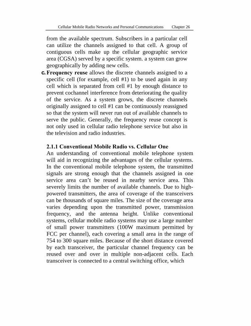
from the available spectrum. Subscribers in a particular cell can utilize the channels assigned to that cell. A group of contiguous cells make up the cellular geographic service area (CGSA) served by a specific system. a system can grow geographically by adding new cells.
c. Frequency reuse allows the discrete channels assigned to a specific cell (for example, cell #1) to be used again in any cell which is separated from cell #1 by enough distance to prevent cochannel interference from deteriorating the quality of the service. As a system grows, the discrete channels originally assigned to cell #1 can be continuously reassigned so that the system will never run out of available channels to serve the public. Generally, the frequency reuse concept is not only used in cellular radio telephone service but also in the television and radio industries.
2.1.1 Conventional Mobile Radio vs. Cellular One An understanding of conventional mobile telephone system will aid in recognizing the advantages of the cellular systems. In the conventional mobile telephone system, the transmitted signals are strong enough that the channels assigned in one service area can’t be reused in nearby service area. This severely limits the number of available channels. Due to high-powered transmitters, the area of coverage of the transceivers can be thousands of square miles. The size of the coverage area varies depending upon the transmitted power, transmission frequency, and the antenna height. Unlike conventional systems, cellular mobile radio systems may use a large number of small power transmitters (100W maximum permitted by FCC per channel), each covering a small area in the range of 754 to 300 square miles. Because of the short distance covered by each transceiver, the particular channel frequency can be reused over and over in multiple non-adjacent cells. Each transceiver is connected to a central switching office, which
Chapter 2 Cellular Mobile Radio Networks and Personal Communications 7
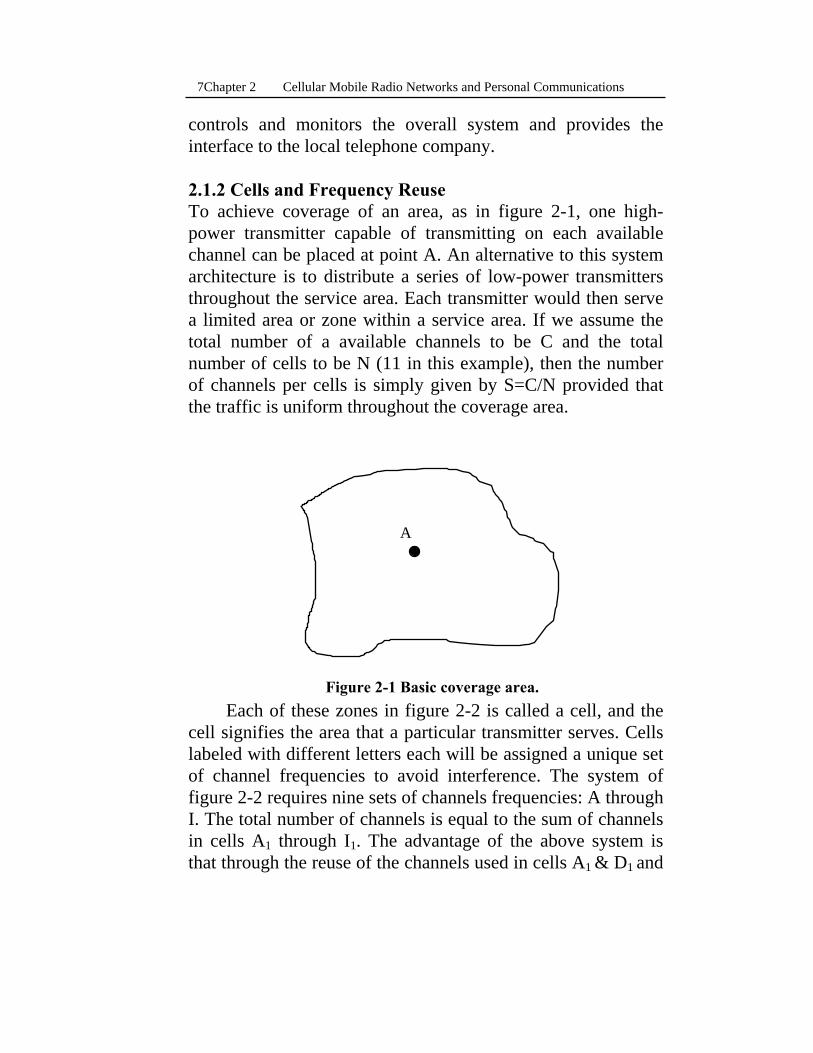
controls and monitors the overall system and provides the interface to the local telephone company. 2.1.2 Cells and Frequency Reuse To achieve coverage of an area, as in figure 2-1, one high-power transmitter capable of transmitting on each available channel can be placed at point A. An alternative to this system architecture is to distribute a series of low-power transmitters throughout the service area. Each transmitter would then serve a limited area or zone within a service area. If we assume the total number of a available channels to be C and the total number of cells to be N (11 in this example), then the number of channels per cells is simply given by S=C/N provided that the traffic is uniform throughout the coverage area.
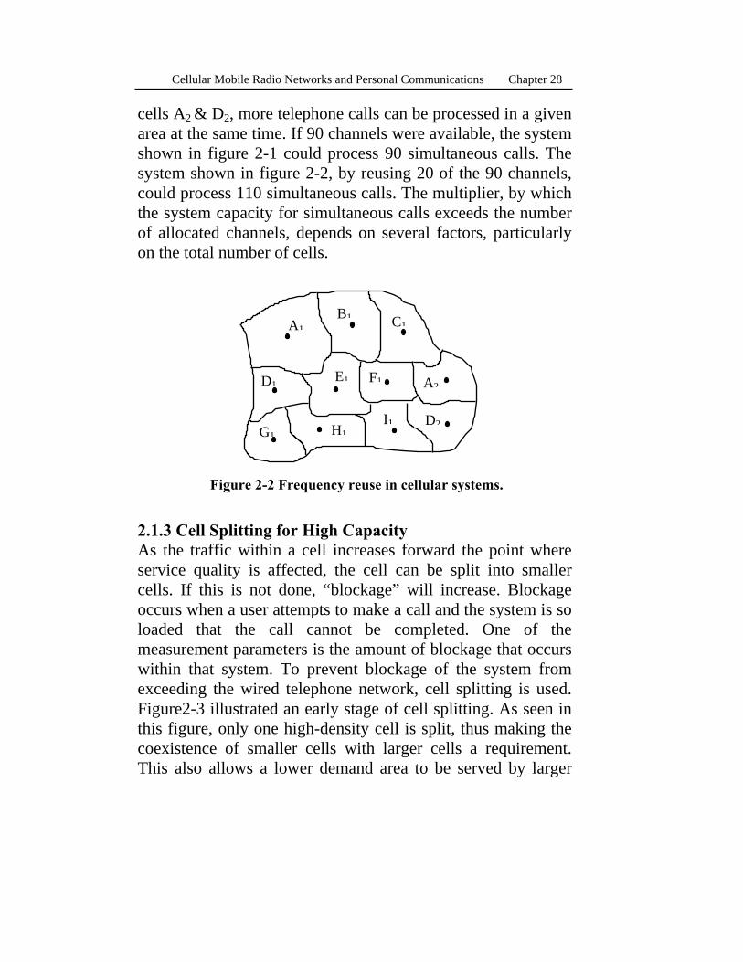
Each of these zones in figure 2-2 is called a cell, and the
cell signifies the area that a particular transmitter serves. Cells labeled with different letters each will be assigned a unique set of channel frequencies to avoid interference. The system of figure 2-2 requires nine sets of channels frequencies: A through I. The total number of channels is equal to the sum of channels in cells A1 through I1. The advantage of the above system is that through the reuse of the channels used in cells A1 & D1 and
A
Figure 2-1 Basic coverage area.
8 Cellular Mobile Radio Networks and Personal Communications Chapter 2
cells A2 & D2, more telephone calls can be processed in a given area at the same time. If 90 channels were available, the system shown in figure 2-1 could process 90 simultaneous calls. The system shown in figure 2-2, by reusing 20 of the 90 channels, could process 110 simultaneous calls. The multiplier, by which the system capacity for simultaneous calls exceeds the number of allocated channels, depends on several factors, particularly on the total number of cells.
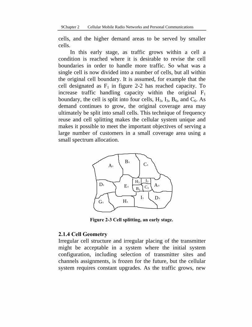
2.1.3 Cell Splitting for High Capacity As the traffic within a cell increases forward the point where service quality is affected, the cell can be split into smaller cells. If this is not done, “blockage” will increase. Blockage occurs when a user attempts to make a call and the system is so loaded that the call cannot be completed. One of the measurement parameters is the amount of blockage that occurs within that system. To prevent blockage of the system from exceeding the wired telephone network, cell splitting is used. Figure2-3 illustrated an early stage of cell splitting. As seen in this figure, only one high-density cell is split, thus making the coexistence of smaller cells with larger cells a requirement. This also allows a lower demand area to be served by larger
B1 C1A1
E1D1
G1
F1
I1H1D2
A2
Figure 2-2 Frequency reuse in cellular systems.
Chapter 2 Cellular Mobile Radio Networks and Personal Communications 9
cells, and the higher demand areas to be served by smaller cells.
In this early stage, as traffic grows within a cell a condition is reached where it is desirable to revise the cell boundaries in order to handle more traffic. So what was a single cell is now divided into a number of cells, but all within the original cell boundary. It is assumed, for example that the cell designated as F1 in figure 2-2 has reached capacity. To increase traffic handling capacity within the original F1 boundary, the cell is split into four cells, H3, I3, B6, and C6. As demand continues to grow, the original coverage area may ultimately be split into small cells. This technique of frequency reuse and cell splitting makes the cellular system unique and makes it possible to meet the important objectives of serving a large number of customers in a small coverage area using a small spectrum allocation. 2.1.4 Cell Geometry Irregular cell structure and irregular placing of the transmitter might be acceptable in a system where the initial system configuration, including selection of transmitter sites and channels assignments, is frozen for the future, but the cellular system requires constant upgrades. As the traffic grows, new
B1 C1A1
B3C3
I3H3E1
D1
G1 I1H1
D2
A2
Figure 2-3 Cell splitting, an early stage.
10 Cellular Mobile Radio Networks and Personal Communications Chapter 2
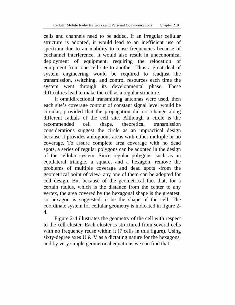
cells and channels need to be added. If an irregular cellular structure is adopted, it would lead to an inefficient use of spectrum due to an inability to reuse frequencies because of cochannel interference. It would also result in uneconomical deployment of equipment, requiring the relocation of equipment from one cell site to another. Thus a great deal of system engineering would be required to readjust the transmission, switching, and control resources each time the system went through its developmental phase. These difficulties lead to make the cell as a regular structure.
If omnidirectional transmitting antennas were used, then each site’s coverage contour of constant signal level would be circular, provided that the propagation did not change along different radials of the cell site. Although a circle is the recommended cell shape, theoretical transmission considerations suggest the circle as an impractical design because it provides ambiguous areas with either multiple or no coverage. To assure complete area coverage with no dead spots, a series of regular polygons can be adopted in the design of the cellular system. Since regular polygons, such as an equilateral triangle, a square, and a hexagon, remove the problems of multiple coverage and dead spots -from the geometrical point of view- any one of them can be adopted for cell design. But because of the geometrical fact that, for a certain radius, which is the distance from the center to any vertex, the area covered by the hexagonal shape is the greatest, so hexagon is suggested to be the shape of the cell. The coordinate system for cellular geometry is indicated in figure 2-4.
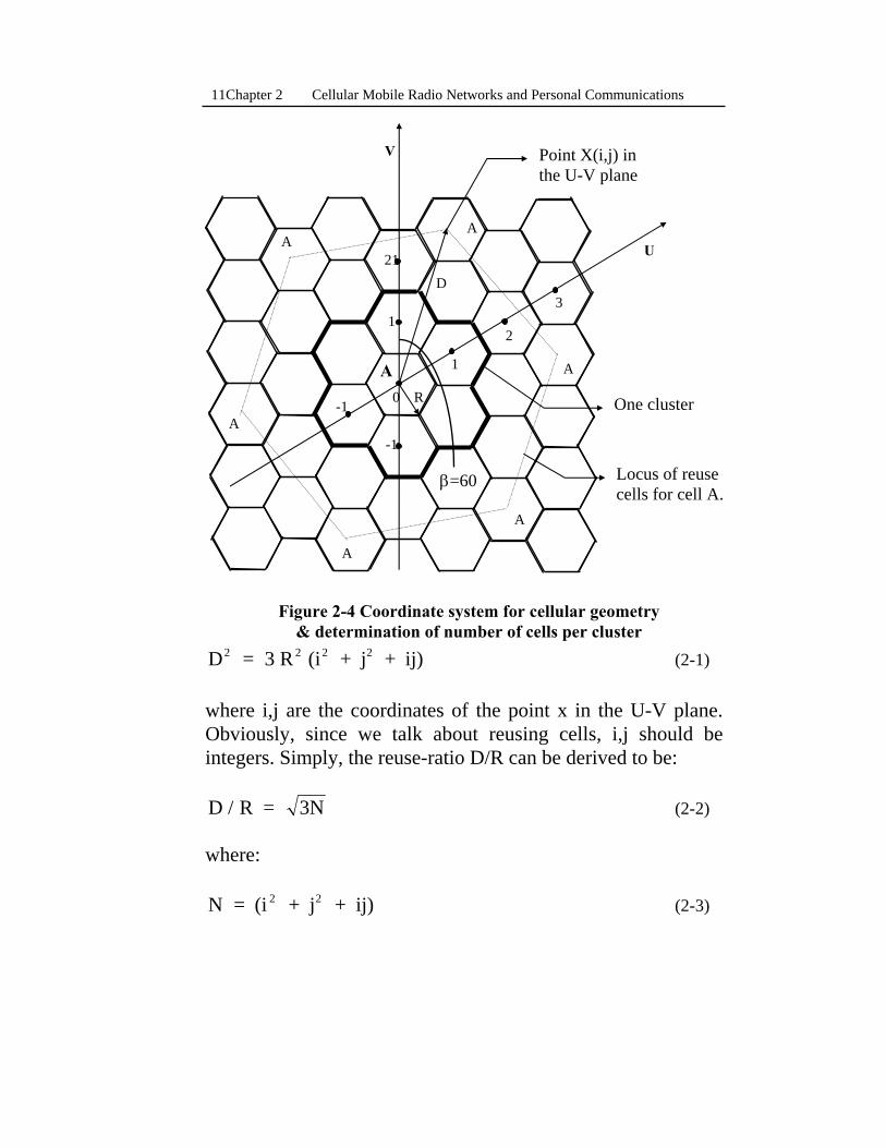
Figure 2-4 illustrates the geometry of the cell with respect to the cell cluster. Each cluster is structured from several cells with no frequency reuse within it (7 cells in this figure). Using sixty-degree axes U & V as a dictating nature for the hexagons, and by very simple geometrical equations we can find that:
Chapter 2 Cellular Mobile Radio Networks and Personal Communications 11
D = 3 R (i + j + ij) 2 2 2 2 (2-1) where i,j are the coordinates of the point x in the U-V plane. Obviously, since we talk about reusing cells, i,j should be integers. Simply, the reuse-ratio D/R can be derived to be: D / R = 3N (2-2) where: N = (i + j + ij) 2 2 (2-3)
Figure 2-4 Coordinate system for cellular geometry & determination of number of cells per cluster
21
31
-1
-1
2
1
0
β=60
V
A
A
A
A
A
A
A
D
R
U
One cluster
Locus of reuse cells for cell A.
Point X(i,j) in the U-V plane
12 Cellular Mobile Radio Networks and Personal Communications Chapter 2
is the number of cells per cluster. In figure 2-4 we have i=1 & j=2 which leads to N=7 and D/R ratio=4.58. But the question is: what is the proper selection for i and j? Alternatively, what is the proper value of D/R? This question is answered by determining the acceptable interference to signal ratio I/S -also known as Interference to Carrier ratio I/C- dictated by the modulation scheme which is given by [1] : I / S = (D / R -1) -n (2-4) where n is the propagation decay law appropriate to the environment. This equation is derived for the worst case S/N ratio. So, approximately I/S could be given by: I / S = (D / R) -n (2-5) Normally, 2≤n≤5. The ratio given by equation 2-5 is due to a one-cell interference. Taking into account the interference caused by all of the six adjacent cells in the cluster leads to: I / S = 6 (D / R) -n (2-6) Considering equation 2-2, we can find that by reducing the D/R ratio the number of cells per cluster is reduced. Assume the total number of RF channels has a constant value C. Then the number of channels per cell is increased; thereby increasing the system traffic capacity. On the other hand, the cochannel interference is increased, according to equation 2-6, as D/R ratio is reduced. The reverse is seen as the ratio D/R is increased.
As stated earlier, the modulation scheme dictates a specific I/S ratio. Hence, the appropriate D/R ratio could be obtained by direct substitution in equation 2-6. The FM modulation employed in analog cellular system dictates I/S

Chapter 2 Cellular Mobile Radio Networks and Personal Communications 13
ratio of -18 dB, hence D/R will be 4.4 resulting in a cluster of 7 cells. On the other hand, efficient digital modulation schemes allow I/S ratio to be -9 dB, hence D/R will be 2.6 resulting in a cluster of 3 cells. These values are obtained by substituting the propagation loss n by 4. 2.1.5 Maximum and Minimum Cell Radius. The maximum radius of a cellular cell is limited by the generated power at the cell site and at the mobile. For the fixed antenna gain and the fixed propagation effects, the cell radius can be increased by transmitting more power. This technique can be successfully used to some extent and the size of the power amplifier (PA) can be increased. However associated with increased sizing of the PA are problems of additional generated noise, cooling, and source power consumption. Obviously, in the case of mobile, dc power consumption cannot exceed a certain value. At the cell sites, as well as at the mobile station, high-power generation imposes special cooling considerations for the power amplifier (obviously, a limit on the maximum rate of cooling also exists). In addition, a high-power transmitter is not of much use once the traffic increases and the initial cells are divided into smaller cells (smaller cells require less power). In cellular systems, effective gain can be increased by increasing the antenna size or by increasing the antenna mast height.
As stated earlier, a cellular system goes through the process of cell division as the traffic demands, in the cell, increase. In most cases, cells carrying high traffic are split in the beginning followed by gradual transformation of other larger cells into smaller cells. The cell division process is such that it divided the original radius of the cell into half. Thus, the area of the new cell is one-fourth of the original cell area. Since the traffic capacity is proportional to the number of new cells, each division increases the capacity by a factor of four.
14 Cellular Mobile Radio Networks and Personal Communications Chapter 2
Thus the maximum traffic capacity of the system can be fixed by the ultimate size of the cell. Since each division increases the system complexity as well as the capacity, the cost per customer remains somewhat unchanged. Though the cell division does not impose additional cost per customer, this process can not go on indefinitely because a smaller cell radius requires frequent handover from one cell site to another as the mobile moves around in the coverage area. This imposes additional hardware requirements. Combining the additional hardware requirements with the necessity of having some tolerance in the position of each transceiver (cell site) due to practical requirements, the practical limit of a one mile radius on cells has been imposed.
2.2 First Generation, analog systems As described in the first chapter, by 1977 there were two carriers in the market, the wireline and the non-wireline. Both of them were sharing the 40 MHz of spectrum allocated by FCC in the 900 MHz band. By 1989, an additional 5 MHz of spectrum were added to each carrier, making the all allocated spectrum to be 50 MHz. If A & B denote the non-wireline and wireline original spectrum respectively, and A\ & B\ denote the additional spectrum, figure 2-5 illustrates the frequency allocation in this band.
The 50 MHz spectrum has been divided into total of 832 full duplex channels, each is 30 KHz band width. Of the 832 channels, 416 channels are assigned to non-wireline and the remaining 416 channels are assigned to the wireline. Among these 832 channels there are 42 control channels. The remaining 790 channels are voice ones.
Before increasing the spectrum to 50 MHz it was 40 MHz all containing 666 full duplex channels denoted by A, B in figure 2-5. These 666 channels contain the 42 control channels (setup channels). This structure remained the same after adding

Chapter 2 Cellular Mobile Radio Networks and Personal Communications 15
the 10 MHz of spectrum. This new spectrum is dedicated to be only voice channels.
2.2.1 Why the 900 MHz Band? The motivation behind the choice of 900 MHz is the availability of proven technology in the UHF band and its ability to penetrate buildings[1]. Furthermore, even in a high electrical noise area, this band is less affected than lower frequencies. Long-range interference caused by ionospheric
50 CHA\
83 CHB\
333 CHB
333 CHA
33 CHA\
50 CHA\
83 CHB\
333 CHB
333 CHA
33 CHA\
45 MHz
891.5846.5 894890880870869849845835825824
RX TX
CH1 CH333 CH334 CH666A B
30 KHz
RCC WCC
666354313 333 3341
(21)(21)
FirstFirstLast Last
Dedicated Control Channels
L to M M to LRCC 869-880
890-891.5 824-835
845-846.5 WCC 880-890
891.5-894 835-845
846.5-849
Figure 2-5 Frequency allocation for the analog system.
16 Cellular Mobile Radio Networks and Personal Communications Chapter 2
changes or by temperature follows an inverse law, with lower frequencies being severely affected and higher frequencies being generally immune to these effects. The antenna size loading effects are considerably reduced because smaller antennas are required at higher frequencies. Also, at this frequency it is possible to make mobile antennas less than a foot in length. Despite these advantages, there are disadvantages in the use of this frequency band for rural areas. For densely cultivated areas with thick vegetation, the attenuation will change considerably with the seasons. In general the direct loss will increase as the obstructions become saturated with moisture or when foliage becomes thick. Obstructions, such as mountains or rain-soaked buildings, often provide effective reflecting areas. Although they affect the direct radio path adversely, the reflected path is often improved. The effect of rain and other atmospherics at this frequency is almost insignificant. 2.2.2 Elements of Analog Cellular Systems There are three elements of a cellular system:
• MTSO, Mobile Telephone Service Office, one per cellular system, which provides for interfacing of the mobile system to the public switched telephone network.
• Cell sites based on the area of coverage, which provides for interfacing between mobile and MTSO
• Mobile users distributed throughout all the cells of a typical cellular system.
The mobile unit communicates to the nearest cell site over
a radio channel assigned to that cell. The cell site is connected to the MTSO by microwave, land cable, or fiber-optic cable, which in turn interfaces with PSTN. All information exchanged over this wireline facility employs standard telephone signaling. Hence, standard switching is required within MTSO. Additionally, MTSO acts as the manager for radio channels

Chapter 2 Cellular Mobile Radio Networks and Personal Communications 17
allocated to different cells, provides coordination between moving subscribers and cell sites, and maintains the integrity of the whole system. Based on the traffic capacity of a particular cell, the number of RF channels are allocated either permanently or temporarily, based on demand. Similarly, the number of voice trunks are connected between a cell site and MTSO.
The data transmission speed of the forward and reverse
setup channels -reserved for controlling the voice channels- in AMPS is 10 Kbps. A single data channel (common control channel, 4-wire) between the cell site and the MTSO carries data at the rate of 2400 bps. The number of voice circuits assigned between the cell site and the MTSO is the same as the assigned number of channels at the cell site. Thus, the cell site does not act as a concentrator. Also, it should be noted that the voice circuits are full duplex. 2.2.3 Call Supervision On the voice channel, one of three tones that modulate the carrier at a low modulation index is used for supervision. These tones are centered at 6 KHz and are termed Supervisory Audio Tones (SAT). The SAT is added to the voice transmission by a cell site. The three frequencies used are 5970, 6000, or 6030 HZ. The function of the SAT is similar to the closing of the local loop in the land telephone system. A given SAT is sent from the cell site to the mobile, which in turn loops back the same SAT to the cell site. The cell-site station must make decisions to determine whether it has received the original transmitted tone, or whether the tone received is different and is the result of some interference. If the SAT is not returned back from the mobile to the cell site it means that, the mobile is fading or it’s transmitter is off.
18 Cellular Mobile Radio Networks and Personal Communications Chapter 2
In addition to SAT , A signaling tone (ST) at a frequency of 10 KHz is transmitted from the mobile to represent mobile user on-hook and off-hook conditions. In addition to the continuous signaling tone at 10 KHz, digital signals are also sent over the voice channel to the mobile user. Data transmission over the forward voice channel is accomplished by a technique known as blank-and-burst. When the cell site wants to send messages to the mobile, the voice signal is blanked for about 50 ms and a burst of 10-Kbps data is inserted in the voice channel. This signaling is used for: alerting the mobile user, disconnection, hold, and handoff.
2.2.4 Locating the Mobile For maintaining good quality voice and data transmission service, a mobile user’s S/I ratio is monitored at the cell site every few seconds. This in turn monitors the cochannel interference. When the call is initially established or when the mobile is switched on, the mobile locates the appropriate cell site by scanning all the control channels (21 paging channels) and selects the one with the highest quality (high S/N ratio). After a call is initially established, the mobile may move out of the original service area. In this condition it may become necessary to reroute the original call through the new cell site, the location of which with respect to the mobile provides a better signal quality. This process of switching the call from one cell site to another is known as handoff and is executed under the control of MTSO. This handoff process can take place several times until the mobile terminates the call. 2.2.5 Mobile Calling Sequence In this section we discuss briefly the calling sequences for a mobile receiver (MR) terminated call , a mobile receiver-originated call, the call releasing sequence, and the handoff sequence.
Chapter 2 Cellular Mobile Radio Networks and Personal Communications 19
2.2.5.1 Mobile-Terminated Call When MTSO receives an incoming call through a standard wireline network, the following scenario occurs:
1. MTSO collects the calling digits, and instructs all cell sites to page the mobile over the forward setup channels.
2. the mobile unit, after recognizing its page, responds to the cell site over the reverse setup channel (access channel).
3. the cell site in turn relays this information to the MTSO over its dedicated landline data link.
4. The MTSO selects an idle voice channel and the associated landline trunk, and informs the cell site of its choice over the appropriate data link (control channel).
5. The serving cell-site inturn tells the mobile of its channel over the forward setup channel.
6. The mobile in turn tunes to the designated voice channel where the SAT signal is present, which is looped back to the cell site.
7. On recognizing the correct looped-back SAT, the cell site places the associated landline trunk in an off-hook state, which the MTSO interprets as a successful voice channel established.
8. On command from MTSO, the cell site transmits a data message over the voice channel to the alerting device at MR, which signals the MR of an incoming call.
9. The signaling tone from the MR causes the cell site to place an on-hook signal over the previously selected landline trunk, which confirms successful alerting to the MTSO.
10.The MTSO, in-turn, provides an audible ring-back tone to the calling party. When the MR answers by going off-hook, ST is removed from the voice channel to the cell site, and in turn activates the off-hook signal on the landline trunk.
11.The off-hook signal is detected at the MTSO, which disables the ring-back tone to the land party and establishes the taking connection.

20 Cellular Mobile Radio Networks and Personal Communications Chapter 2
It should be noted that up to the point of SAT turnaround by mobile, all communication between the MTSO and CS (Cell Site) is over the data link. Communication between the cell site and the MR is over the voice channel after voice channel assignment. 2.2.5.2 Mobile-Originated Call Using the pre-origination dialing procedure, the mobile user enters the dialed digit into the equipment’s memory and the following steps occurs:
1. The stored digits, along with the mobile’s own identification, is transmitted to the cell site through the reverse setup (access channel) channel.
2. The cell site receives this information and relays it to the MTSO.
3. A voice channel is selected by the MTSO and the cell site is informed.
4. The cell site then informs the mobile about the voice channel designation.
Similar to the mobile-terminated call , the MTSO extends the connection to the PSTN after confirming the SAT of the calling mobile. The conversation can begin when the called party answers. 2.2.5.3 Mobile-Initiated Release The mobile initiates the releasing sequence by going on-hook (or END button is depressed). The following steps occur:
1. The supervisory tone on the voice channel is turned on, which is received by the cell site.
2. The presence of ST and SAT indicates the on-hook condition of the mobile at the cell site. As a result, the cell site places an on-hook signal on the appropriate landline trunk towards the MTSO.
Chapter 2 Cellular Mobile Radio Networks and Personal Communications 21
3. On receipt of the on-hook signal, the MTSO idles all switching office resources and transmits any necessary disconnect signals through the wireline network. The MTSO also commands the previously serving cell site over its data link to shut down the cell-site radio transmitter. Any equipment used at this time is then free to be used in a new call. 2.2.5.4 Land Subscriber-Initiated Release When the call release is land-subscriber initiated, an on-hook signal is transmitted from the land mobile network and:
1. the MTSO idles all the switching office resources associated with the call to be released. The MTSO sends a data message over the data link to the serving cell site.
2. The cell site in turn sends the release message to the mobile over the voice channel.
3. The mobile then responds to the release order from the cell site by turning on the supervisory tone.
4. Upon receipt of the supervisory tone, the on-hook signal is initiated by the cell site towards the MTSO over the appropriate landline trunk. Finally, and after receiving the on-hook signal, the MTSO idles all the equipment.
2.2.5.5 Handoff Handoff, in general, is the process of switching over a call path from its old cell site to a new cell site when the voice signal drops below a certain minimum value. As the user moves from cell to cell, he is assigned a new channel with each move. With a deteriorating signal-to-noise ratio at the cell site, the switch-over can also take place within the same cell. The location information gathered by serving the cell site and other cell sites is transmitted to the MTSO over the landline trunks. When the carrier drops below a certain level, the MTSO decides to switch over the present call from the old cell site to the new one.
22 Cellular Mobile Radio Networks and Personal Communications Chapter 2
2.3 Second Generation (GSM standards), digital systems, the current cellular The Pan-European digital cellular system traces its origins to 1982, when analog cellular services were in their earliest stages of commercial deployment. At that early date, European authorities anticipated the long-term potential of mobile communications and stimulated CEPT, the Conference of European Postal and Telecommunications administrations, to study the creation of a mobile telephone standard to be adopted throughout Western Europe. CEPT responded by forming the Groupe Special Mobile. Group members used the initials GSM to refer to their project. At the very beginning, GSM had two objectives:
• Pan-European roaming, which offers compatibility throughout the European continent.
• interaction with the integrated service digital network (ISDN), which offers the capability to extend the single-subscriber-line system to a multi-service system with various services which are currently offered only through diverse telecommunications networks.
Later, the project formally adopted a broad set of aims, which included:
• full international roaming • provision for national variations in charging and rates • efficient inter-operation with ISDN systems • signal quality better than or equal to that of existing mobile
systems • traffic capacity higher than or equal to that of present
systems • subscriber costs lower than or equal to those of existing
systems • accommodation of non-voice services • accommodation of portable terminals
Chapter 2 Cellular Mobile Radio Networks and Personal Communications 23
2.3.1 GSM Architecture In this section we will briefly discuss the basic components and architecture of the GSM system. 2.3.1.1 Mobile Station The MS may be a stand-alone piece of equipment for certain services or support the connection of external terminals, such as the interface for a personal computer or fax. The MS includes:
• Mobile Equipment (ME), which is subscriber-independent. • Subscriber Identity Module (SIM), which stores all the
subscriber-related information and it can be inserted in any ME. SIM is which identifies the subscriber. 2.3.1.2 Base Station Subsystem The Base Station Subsystem (BSS) mainly consists of:
• Base Transceiver Station (BTS), which is located at the antenna site. It consists of radio transmission and reception equipment similar to the ME in an MS.
• Base Station Center (BSC), which may control several BTSs. 2.3.1.3 Network and Switching Subsystem The NSS includes the main swithcing functions of GSM. The NSS management consists of:
• Mobile Service Switching Center (MSC), which coordinates call set-up to and from GSM users. One MSC controls several BSCs.
• Inter-working Function (IWF), which is a gateway for MSC to interface with external networks for communication with users outside GSM, as exists in the new design for the UMTS (see section 2.4.3.2).
• Home Location Register (HLR), which consists of a stand-alone computer without switching capabilities, a database which contains subscriber information, and information
24 Cellular Mobile Radio Networks and Personal Communications Chapter 2
related to the subscriber’s current location, but not the actual location of the subscriber.
• Authentication Center (AUC), which is considered to be a supplemental part to the HLR. The AUC manages the security data for subscriber authentication.
• Equipment Identity Register (EIR), which stores the data of the ME unit.
• Visitor Location Register (VLR), which may link to more than one MSC. VLR stores more location subscriber information than HLR such as the current location.
• Gateway MSC (GMSC), which finds the correct HLR by knowing the directory number of the GSM subscriber. 2.3.2 Radio Transmission GSM networks presently operate in three different frequency ranges [7]. These are:
• GSM 900 (also called GSM)- operates in the 900 MHz frequency range and is the most common in Europe and the world.
• GSM 1800 (also called PCN standing for Personal Communications Network and called DCS 1800 standing for Digital Cellular System)- operates in the 1800 MHz frequency range and is found in a rapidly-increasing number of countries including France, Germany, Switzerland, the UK, and Russia.
• GSM 1900 (also called PCS standing for Personal Communication Services, PCS 1900, and DCS 1900)- the only frequency used in the United States and Canada for GSM.
As in the analog system described in the first section, there are two 25 MHz bands separated by 45 MHz, with the lower band used for transmissions from terminal to base stations and the upper band for transmission from base stations to terminals.
Chapter 2 Cellular Mobile Radio Networks and Personal Communications 25
2.3.2.1 Physical Channels The GSM system uses the Time Division Multiple Access technique (TDMA) described in next chapter. Meanwhile, with 200 KHz carrier spacing, the frequency allocation of 25 MHz per direction admits the possibility of having 125 carriers per direction. However, GSM specifies only 124 carriers, leaving unoccupied guard bands at the edges of the GSM spectrum allocation. 2.3.2.2. Slow Frequency Hopping GSM has two definitions of radio carriers. One is the conventional definition of a sine wave at a single frequency (among the 124 stated carriers). The other definition of a radio carrier is a frequency hopping pattern, consisting of a repetitive sequence of frequencies occupied by a signal. When the radio carrier is a frequency hopping pattern, the signal moves from one frequency to another in every frame. Without frequency hopping, the entire signal is subject to distortion whenever the assigned carrier is impaired. Also frequency hopping can reduce the harmful effects of cochannel interference between signals in nearby cells. 2.3.2.3 Radiated Power GSM specifies five classes of mobile stations distinguished by maximum transmitter power, ranging from 20W to 0.8 W. Typically, the maximum power capability of vehicle-mounted terminals is 8W (on average 1W). Portable terminals typically have 2W maximum power (on average 250mW). In common with other cellular systems, GSM employs power control. On the other hand, terminals can adjust their power to any of 16 power levels that range over 30 dB in steps of 2 dB.
26 Cellular Mobile Radio Networks and Personal Communications Chapter 2
2.3.3 Security in GSM Security in GSM is handled through two ways, the authentication process, and the encryption for user data transfer[3]. 2.3.3.1 Authentication Authentication protects the network against unauthorized access and it is achieved in two phases.
• Phase 1: A PIN (Personal Identification Number) code protects the SIM from unauthorized use. When powering the ME on, the user is requested to enter his PIN number and it should match that one of the SIM card. If the PIN is entered incorrectly three consecutive times the SIM will be blocked, and the unlocking code should be requested from the network operator.
• Phase 2: When SIM is issued, a “Ki” key is stored on the card, and in the network authentication center (AUC), home location register (HLR), and the visitor location register (VLR). To make a call, the handset must be authenticated, which is accomplished in this manner:
1. Network send a 128-bit random number (RAND) to the handset, which passes it to the SIM card.
2. SIM card computes a 32-bit signature response (SRES) using RAND, A3 algorithm, and Ki key for the handset.
3. Network receives SRES from handset and repeats calculation to verify subscriber’s identity.
For security reasons, the Ki key never leaves the SIM card, and is never sent over the network. If the calculation agrees, the connection continues and the base station sends the handset its temporary mobile subscriber identity (TMSI); if it fails, the connection is terminated with an authentication failure message.
Chapter 2 Cellular Mobile Radio Networks and Personal Communications 27
2.3.3.2 Encryption To encrypt signaling and voice channel data, the SIM card computes a 64-bit ciphering key (Kc) for the handset using RAND, A8 algorithm, and Ki key. This calculation is also performed in the network to recover the Kc key. All communications between the handset and base station can now proceed using this Kc key and the A5 algorithm, once a ciphering mode request has been received from the network by the handset. Additional security to foil eavesdroppers may be accomplished by changing the ciphering key during the connection or at hand-off time to a new base station. 2.3.4 Roaming Roaming is the ability to use your own GSM phone number in another GSM network. A roaming agreement is a business agreement between two network operators to transfer items such as call charges and subscription information back and forth, as their subscribers roam into each others areas.
If roaming is made to another county whose network woks at a different GSM frequency, the ME is no longer usable unless it is dual band which operates in the both frequency bands of the two networks. Otherwise, the SIM card should be transferred to another ME, the matter that reserves for the user his complete identification, since identification in the GSM network is accomplished by the SIM card not by the ME or the MS units. 2.4 Third Generation, Universal Mobile Telephone System (UMTS),the future While no one can predict the future, it is very near that -may be at the start of the twenty first century- the way the world communicates will be vastly different from now [15]. A very intensive research and standardization activity is underlying the basic design of third-generation systems targeted for completion around the year 2000.
28 Cellular Mobile Radio Networks and Personal Communications Chapter 2
Standardization is ongoing for third-generation systems in the European Telecommunication Standardization Institute (ETSI), under the project name Universal Mobile Telecommunication Systems (UMTS) and in the International Telecommunications Union (ITU), where it is called IMT2000. 2.4.1 Motivations Behind (UMTS) The tremendous growth of Internet usage is the main driver for third-generation wireless [15], but it is not alone. The most important factors driving the development, the start-up, and deployment of such an innovative mobile system, UMTS, come from the following [2]:
• New service requirements that cannot be satisfied with pre-UMTS systems.
• The functional and resource-sharing advantages based on the integration of mobile and fixed networks.
• Prospective business opportunities associated with UMTS. • The incumbent capacity shortage, and the need for a more
efficient spectrum use. 2.4.2 Requirements and Different Points of View. The UMTS service and networks transition paths are heavily conditioned by the vies and plans of four major players acting in the future telecommunications landscape: the customer, the service provider, the network operator, and the regulator. 2.4.2.1 The Customer Requirements Users demand new features and capabilities which can be summarized in:
• Seamless Internet/Intranet access • Multimedia communication capabilities • Inexpensive, lightweight terminal • Low tariffs over a wide range of bearer services • User-friendly access to services
Chapter 2 Cellular Mobile Radio Networks and Personal Communications 29
2.4.2.2 The Network Operator/Service Provider Viewpoint The consumer demand will drive the actions to be taken by the operators/service providers. As an example, in recent years, European GSM operators have been directing the majority of their investment to enhance the performance (coverage and capacity) of their expensive base station system (BSS). Now that the coverage process is approaching a more stable situation, most of the large European operators are moving their attention to the enhancement of the available services and network features. Generally, operators are showing a strong interest for the following:
• A radio access part that minimizes the deployment costs under quality of service (QoS) constraints.
• A capacity improvement through new radio technology. • A flexible network architecture that permits equipment reuse
for both fixed and mobile services. 2.4.2.3 The Regulator Viewpoint The aim of the regulator is to:
• Develop a multi-operator/multi-service provider regime to guarantee competition
• Manage effectively the available spectrum inside a competitive context
• Ensure a fair play among all license holders 2.4.3 New Technology and Standardization Actually, due to the limited bandwidth currently available, it seems difficult that UMTS on its own could provide both narrow-and wide- band services to a growing market. In addition to the basic voice service, UMTS should also support bearers with higher bandwidths than GSM can provide.
Steps were already taken, while others are still in the processes of standardization and suggestion to achieve the new communication approach.
30 Cellular Mobile Radio Networks and Personal Communications Chapter 2
2.4.3.1 Wide-Band CDMA In January 1998, ETSI (European Telecommunications Standard Institute) decided to base the UMTS standard on a new wide-band technology, WCDMA, using 5-MHz wide-band radio carriers. This WCDMA radio-access technology supports instant access to wireless multimedia optimized for packet-switched data. This is a totally new approach to CDMA technology and inherently different from previously proposed narrow-band CDMA systems such as IS95, which was primarily designed for voice communication.
The new generation, along with it’s new multiple access technology, will be in the 2 GHz frequency band, (the 1920-1980 MHz band, paired with 2110-2170 MHz), which was allocated at the 1992 World Administrative Radio Conference for third generation UMTS/IMT2000 services in Europe and Asia. 2.4.3.2 Dual Air-Interface Following the successful standardization process for GSM, European research started in the late 1980’s to develop the UMTS air interface standard. This new air interface standard, together with an evolved GSM core network, will from a UMTS/IMT2000 standard. The core network is retained with its network signaling parts, etc.
UMTS aims to deliver wide-area/high-mobility data rates of 384 kbps, and up to 2 Mbps for local-area/low-mobility coverage. To reach this level of throughput, two air interface will coexist [15]: the evolved GSM and the new UMITS interface. And using dual-mode GSM/UMTS global handsets- with GSM providing coverage and UMTS delivering new functionality- operators will be able fully to leverage additional wide-band services in their GSM networks with full service transparency across the enormous GSM worldwide presence.

Chapter 2 Cellular Mobile Radio Networks and Personal Communications 31
2.5 Personal Communications What we have discussed in the previous sections is a way to implement a wider concept, the personal communications. In a broad sense and generally speaking, personal communications begin with a person. Mobility is at the heart of personal communications. People transmit and receive information wherever they are and whenever they choose, even when they are moving. They want to produce and acquire information in formats they choose-including sounds, text, still pictures, moving pictures, keyboard operations, mouse movements, and pen strokes. The promise of personal communications is to make all kinds of information available anywhere, anytime, at low cost to a large mobile population. 2.5.1 What Is a Personal Communications System? From what introduced above, we can define the personal communications system to be: “A personal communications system provides people with wireless access to information services”[4]. This is a deliberately broad definition that applies to a wide variety of existing and future systems, including residential cordless telephones, cellular networks, and mobile data networks. Of course, it also includes Personal Communications Services and Personal Communications Networks, which are the official designations of systems operating in specific geographical areas and frequency bands, established by government regulators. In fact, the main distinguishing characteristic of the official PCSs and PCNs is their treatment by authorities. In terms of technologies and services offered, many of them are virtually identical to cellular telephone systems. 2.5.2 Key Attributes of Personal Communications From the point of view of the human user, the key attributes of advanced personal communications are listed below.
32 Cellular Mobile Radio Networks and Personal Communications Chapter 2
User Mobility First of all, and as an aim of the Personal Communications, the user mobility is the most important attribute in the personal communications from the user point of view. Personal Information Machine (PIM) it is the name given in [4] to the information device carried by the person. Like a telephone, PIMs will have a microphone, an earphone, and a keypad. It will also have a display screen. It will be comfortable to carry. Personal Address This replaces a person’s conventional telephone numbers. Each conventional telephone number is associated with a specific location, such as the person’s residence, office, or vehicle. A personal address, by contrast, remains with the person as he changes location. Personal Profile One component of the personal profile is a directory with the names and personal addresses of people frequently called. The personal profile also contains details of services selected by the subscriber, which may include calling party identification, voice mail, and selective call forwarding. Advanced profiles will automatically examine arriving information and process it according to the subscriber's preferences. All locations Personal information services will be available in all locations. Subscribers will maintain communications as they change location. Multiple Information Formats Personal information services will accept and deliver information in the formats selected by the users themselves.
Chapter 2 Cellular Mobile Radio Networks and Personal Communications 33
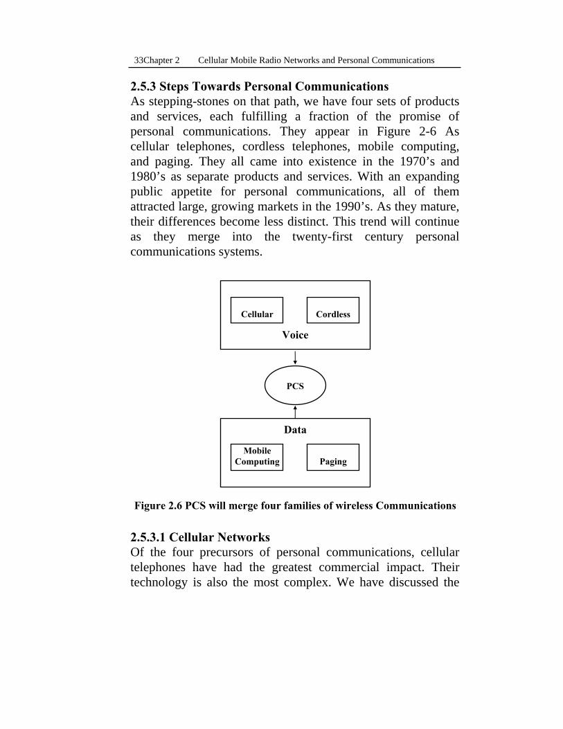
2.5.3 Steps Towards Personal Communications As stepping-stones on that path, we have four sets of products and services, each fulfilling a fraction of the promise of personal communications. They appear in Figure 2-6 As cellular telephones, cordless telephones, mobile computing, and paging. They all came into existence in the 1970’s and 1980’s as separate products and services. With an expanding public appetite for personal communications, all of them attracted large, growing markets in the 1990’s. As they mature, their differences become less distinct. This trend will continue as they merge into the twenty-first century personal communications systems. 2.5.3.1 Cellular Networks Of the four precursors of personal communications, cellular telephones have had the greatest commercial impact. Their technology is also the most complex. We have discussed the
PCS
Data
Mobile Computing
Paging
Voice
Cellular
Cordless
Figure 2.6 PCS will merge four families of wireless Communications
34 Cellular Mobile Radio Networks and Personal Communications Chapter 2
main aspect of the cellular mobile radio networks in the previous sections. 2.5.3.2 Cordless Telephones In contrast to cellular systems, which are complete communications networks, residential cordless phones simply replace the telephone line cord with radio equipment that transmits signals between a telephone and the pair of telephone company wires within a residence. Each country establishes spectrum bands for cordless telephone operation. However, there is no need for compatibility standards governing residential cordless telephone operation.
Residential cordless telephones are important stepping-stones to personal communications because they have attracted a mass market of consumers who have come to appreciate the convenience of using their phones where they choose within their homes. The main limitation of a cordless telephone is that it functions only within a limited distance from a single residential base station. 2.5.3.3 Mobile Computing It can be argued that personal computing was the most significant development in information technology in the 1980’s. Since the early 1990’s two powerful trends have propelled advances in personal computing. One is the popularity of portable computers: laptops, notebooks, and personal digital assistants. The other major trend in personal computing is networking.
The simultaneous popularity of portable computing and networking poses a paradox, because portable computers are disconnected from the wires of conventional networks and from public power supplies. But by making use of wireless data networks, the owners of portable computers retain the advantages of mobility and they remain connected to their important information services.
Chapter 2 Cellular Mobile Radio Networks and Personal Communications 35
2.5.3.4 Paging Paging is the oldest of the personal communications precursors. It is also the simplest technically, and as a consequence the least expensive. Paging is a one-way service. All information travels from the network infrastructure to users. Another reason why paging is relatively simple is that the base stations have high power budgets leading to coverage areas hundred or thousands of times greater than those of cellular, cordless, or wireless data base station.
Chapter 3
Multiple Access and Channel Assignment for Spectral Efficiency
he efficient use of the spectrum is the most important problem in mobile communications [6]. The market for cellular radio services is expected to increase dramatically
this decade. Service may be demanded by 50 percent of the population. The fulfillment of this demand is beyond what can be accomplished with the presently used analog cellular system. Digital technology, modulation, multiple access techniques, and channel assignment are being developed to improve spectrum utilization.
Here, in this chapter, we will give an over view for the different techniques of multiple access and discuss briefly the main features of the channel assignment problem (CAP). The word “Channel” has more than one use which can lead to a misunderstanding, accordingly in this chapter this will be explained. 3.1 Multiple Access Techniques. As introduced, because of the frequency spectrum is a limited resource, we should utilize it very effectively. In order to approach this goal, spectrum efficiency should be clearly defined from either a total system point of view or a fixed point-to-point link perspective. For most radio systems, spectrum efficiency is the same as channel efficiency, the maximum number of channels that can be provided in a given frequency band. This is true for a point-to-point system that does not reuse frequency channels such as a cellular mobile radio. An appropriate definition of spectrum efficiency for cellular mobile radio is the number of channels per cell [16].
T

Chapter 3 Multiple Access and Channel Assignment for Spectral Efficiency 37
The objective of multiple access techniques is to combine signals from different sources onto a common transmission medium in such a way that, at the destinations, the different channels can be separated without mutual interference. In other words, multiple access systems permit many users -each channel is dedicated to each user- to share a common medium in the most efficient manner as away to increase the number of users per cell, accordingly, the spectrum efficiency. There are three main types of the multiple access techniques described below. 3.1.1 Frequency Division Multiple Access (FDMA). FDMA systems allow for a single mobile telephone to call on a radio channel. Typically FDMA systems use analog FM radio modulation but occasionally will use digital phase modulation. FDMA systems typically have a control channel which coordinates radio channel assignment to a voice channel. After the mobile telephone coordinates its access on the control channel, the cellular system assigns it to a voice channel, however; each voice channel can communicate with only one mobile telephone at a time. Figure 3-1 illustrates the FDMA system.
Voice Circuit for One User
Voice Circuit for One User
Control Circuit
Time
f1
f2
fn
.
.
.
.
.
.
.
.
.
.
.
.
.
.
.
.
.
.
.
.
.
.
.
.
.
.
.
.
.
.
.
.
.
.
.
.
.
.
.
.
.
.
Carrier Frequency
Domain
Figure 3.1 A typical FDMA system.
38 Multiple Access and Channel Assignment for Spectral Efficiency Chapter 3
While FDMA systems do not allow more mobile telephones to share a single radio channel, it is possible to increase the number of channels that can be placed in a cell site by reducing the radio channel bandwidth.
Typically, in the U.S. system with FDMA technique the whole spectrum is 50 MHz for the two carriers wireline and non-wireline (refer to chapter 2). Each carrier has a 25-MHz of the spectrum. Due to a full duplex system, a 12.5 MHz bandwidth for transmission with 30 KHz for each channel leads to 416 channels, where 21 of them are dedicated to the paging channels this leads to 395 users per cluster. Dividing this number by 7 cells/cluster leads to have 56 users per cell.
Advantages of FDMA: FDMA mobile telephones typically cost less than digital mobile telephones because they are relatively simple to design and as a result large quantities are being produced. Nevertheless, with the continued integration of digital circuits, the cost of FDMA mobile telephones may eventually be equal to or even more expensive than digital mobile telephones. Disadvantages of FDMA: Non efficient utilization for the spectrum which leads to a small number of users accessing the system through one cell. 3.1.2 Time Division Multiple Access (TDMA). TDMA systems allow several mobile telephones to communicate simultaneously on a single radio carrier frequency. These mobile telephones share the radio frequency by dividing their signal into time slots. Time slots can then be dedicated or dynamically assigned.
TDMA systems divide the radio spectrum into radio carrier frequencies typically spaced 30 KHz to 200 KHz apart. This spacing between the carrier frequencies is the nominal or effective bandwidth of the total multi-channel multiplexed
Chapter 3 Multiple Access and Channel Assignment for Spectral Efficiency 39
signal. TDMA systems typically have narrowband radio voice or traffic channels but can have wideband radio signals. In an FDMA system, the bandwidth of a radio signal waveform is the same thing as the bandwidth of a radio channel, since there is only one channel using the entire signal waveform. In TDMA and CDMA system, a channel is not the same thing as an entire signal waveform, but is instead only a part of it.
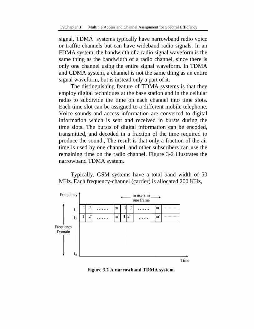
The distinguishing feature of TDMA systems is that they employ digital techniques at the base station and in the cellular radio to subdivide the time on each channel into time slots. Each time slot can be assigned to a different mobile telephone. Voice sounds and access information are converted to digital information which is sent and received in bursts during the time slots. The bursts of digital information can be encoded, transmitted, and decoded in a fraction of the time required to produce the sound., The result is that only a fraction of the air time is used by one channel, and other subscribers can use the remaining time on the radio channel. Figure 3-2 illustrates the narrowband TDMA system.
Typically, GSM systems have a total band width of 50
MHz. Each frequency-channel (carrier) is allocated 200 KHz,
Frequency
Time
f1 f2
fn
.
.
.
.
.
.
.
.
.
.
.
.
.
.
.
.
.
.
.
.
.
.
.
.
.
.
.
.
.
.
.
.
.
.
.
.
.
.
.
.
.
.
Frequency Domain
Figure 3.2 A narrowband TDMA system.
……. 2 1 m ……. 2 1 m ………………
……. 2\1\ m\ ` ……. 2\1\ m\ ………………
m users in one frame

40 Multiple Access and Channel Assignment for Spectral Efficiency Chapter 3
this leads to have 125 carriers. Leaving one channel to be a guard space this leads to 124 carriers. Each frame constitutes of 8 users, so 8 users utilize the same carrier. From chapter 2 it was calculated that the number of cells per cluster in digital modulation systems is 3 cell/clusters. Accordingly, the number of users per cell per MHz of bandwidth equals to (8 x 124)/(3 x 50) = 6.61 users/cell/MHz. But to compare the results with the FDMA whose band width is half of that of the GSM systems, we will consider the GSM to has only a 25 MHz bandwidth. This leads to 6.61 x 25 = 165 users/cell. If compared to the FDMA (56 users/cell) it is greater than by a factor of 2.53. Advantages of TDMA
• Because TDMA allows multiple circuits per carrier, money can be saved on transmitters at the cell sites.
• Burst transmission impacts positively on the cochannel interference because at any given moment, only a part of the mobiles are transmitting, leading to better frequency reuse.
• No duplexers are required, saving money. These can be replaced with fast switches to turn the transmitters and receivers on and off.
• TDMA is flexible, that is, as speech-coding algorithms improve, the TDMA channel is reconfigurable. Disadvantages of TDMA.
• The TDMA mobile requires more complex signal processing hardware. However, as VLSI advances, this may become a non-problem.
• The TDMA receiver must resynchronize on each burst. Also, because unequal propagation delays may cause one user to slip into another user’s slot, TDMA needs a larger overhead than FDMA, which could be a penalty of as much as 30 percent of the total bits transmitted [6].
Chapter 3 Multiple Access and Channel Assignment for Spectral Efficiency 41
3.1.3 Code Division Multiple Access (CDMA). CDMA technology differs from TDMA technology in that it divides the radio spectrum into wideband digital radio signals with each signal waveform carrying several different coded channels. Each coded channel is identified by a unique Pseudo-random Noise (PN) code. Digital receivers separate the channels by correlating (matching) signals with the proper PN sequence and enhancing the correlated one without enhancing the others. The CDMA RF signal waveform uses some of its coded channels as control channels. The control channels include a pilot, synchronization, paging, and access channel.
The base station uses a wide CDMA RF signal waveform which provides for many different coded channels. Some of these coded channels are used for control and access coordination and others are used for voice communications. The CDMA mobile telephone accesses the system either through an analog control channel or coded channel on the CDMA RF signal waveform. When the mobile telephone obtains access on the CDMA system, the CDMA control channel responds by assigning the CDMA mobile telephone to a new coded channel. This is typically on the same RF carrier frequency.
To calculate the maximum number of users per cell in the
case of CDMA, let us assume that a single physical channel (carrier) occupying the whole available bandwidth of the system is allocated to all users in one cell configuration. Let us also assume that the power control is exercised by the mobile such that the received powers of all mobiles at the cell site are the same. In this case the cell site receiver processes a composite signal of all mobiles containing the desired signal power of P and (N-1) interfering signals, each having the power of P. Thus the C/I ratio is given by:
42 Multiple Access and Channel Assignment for Spectral Efficiency Chapter 3
CI
PP N N
=−
=−( ) ( )11
1 (3-1)
But CI
EI
RW
b=⎛⎝⎜
⎞⎠⎟⎛⎝⎜
⎞⎠⎟0
(3-2)
where, R is the information bit rate of the desired user and W is the total spread bandwidth of the system and Eb/I0 is the bit energy-to-interference density ratio. By neglecting the thermal noise, solving the two equations simultaneously leads to: EI
W RN
b
0 1=
−/
( ) (3-3)
Two techniques can increase the number of users [1], one based on natural behavior of speech and second based on antenna sectorization. Studies have shown that on the average a speaker only talks for about 40% of the time. Thus, for the remaining period of the time the interference induced by the speaker is eliminated. Since the channel is shared between all users, noise induced in the desired channel is reduced due to the silent interval of other interfering channels. On the other hand, assuming a 120-degree sectored antenna at the cell site, the interference sources seen by any antenna are roughly one-third of those seen by an omnidirectional cell-site antenna. Accounting for both speech activity and antenna sectorization, (3-3) can be modified to be: EI
W RN
b
0
31
=−⎛
⎝⎜⎞⎠⎟
/
α (3-4)
Chapter 3 Multiple Access and Channel Assignment for Spectral Efficiency 43
where α is the speech activity factor, which usually has an approximate value of 0.4.
Typically, the U.S digital system has an allocated bandwidth of 12.5 MHz. Assuming 8-Kbps digitized speech and Eb/I0 ratio of 7 db, substituting in (3-3) leads to N=312 users/cell. Comparing this number by the 56 users/cell for the FDMA indicates an increasing by a factor of 5.57. But substituting in 3-4 gives the overall increasing factor which is approximately 5.57 x 1/0.4 x 3=42.
It should be noted here that we have allocated the total
bandwidth to a single channel. In reality, there will be several spread-spectrum channels. In other words, the total bandwidth of 12.5 MHz may be divided equally between, for example, half a dozen channels [1].
Advantages of CDMA
• CDMA is the only multiple access technique that takes advantage of the voice activity cycle to increase capacity.
• Only a correlator is necessary at the receiver as opposed to an equalizer, which simplifies cost.
• Only one radio is needed at each cell site, saving money. • No guard time is necessary in CDMA. • Less fading occurs because of the wideband used. • Soft capacity: all users share one channel; additional users
can be added with minor degradation. Disadvantages of CDMA Higher in cost than the FDMA and TDMA since these two systems have been produced and operated for several years. But with evolving technology this will not be an obstacle, specially when the Wide-band Code Division Multiple Access (WCDMA) becomes the technique of the third generation [15].

44 Multiple Access and Channel Assignment for Spectral Efficiency Chapter 3
3.2 Channel Assignment The terms “frequency management” and “channel assignment” often create some confusion [16]. Frequency management refers to designating set-up channels and voice channels (done by the FCC), numbering the channels (done by the FCC), and grouping the voice channels into subsets (done by each system according to its preference). Channel assignment refers to the allocation of specific channels to cell sites and mobile units. The frequency management function is discussed in sec. 2.1.
Here in this section we are interested in demonstrating an overview of the most common solutions for the channel assignment problem (CAP). The most common channel assignment scheme is the fixed channel assignment (FCA). On contrary, there is the Dynamic Channel Assignment (DCA) which has shortcomings rather than the (FCA). To avoid the disadvantages of the (DCA) scheme, improvements are made to enhance the (FCA). 3.2.1 Fixed Channel Assignment The most widely used channel assignment scheme in today’s cellular systems is the Fixed Channel Assignment (FCA). This is due to its simplicity and its moderate requirements of centrally controlled operations. Therefore, it has also been widely considered as a bench mark policy when evaluating other channel assignment techniques [17].
In FCA, channels are assigned to each cell site for relatively long periods of time, in a manner respecting the reuse constraints. So the problem concerns the adjacent-channel assignment which includes neighboring-channel assignment and next-channel assignment. Therefore, within a cell we have to be sure to assign neighboring channels in an omnidirectional-cell system and in a directional-antenna-cell system properly. In an omnidirectional-cell system, if one channel is assigned to the middle cell of seven cells, next channels cannot be assigned in the same cell. Also, no next
Chapter 3 Multiple Access and Channel Assignment for Spectral Efficiency 45
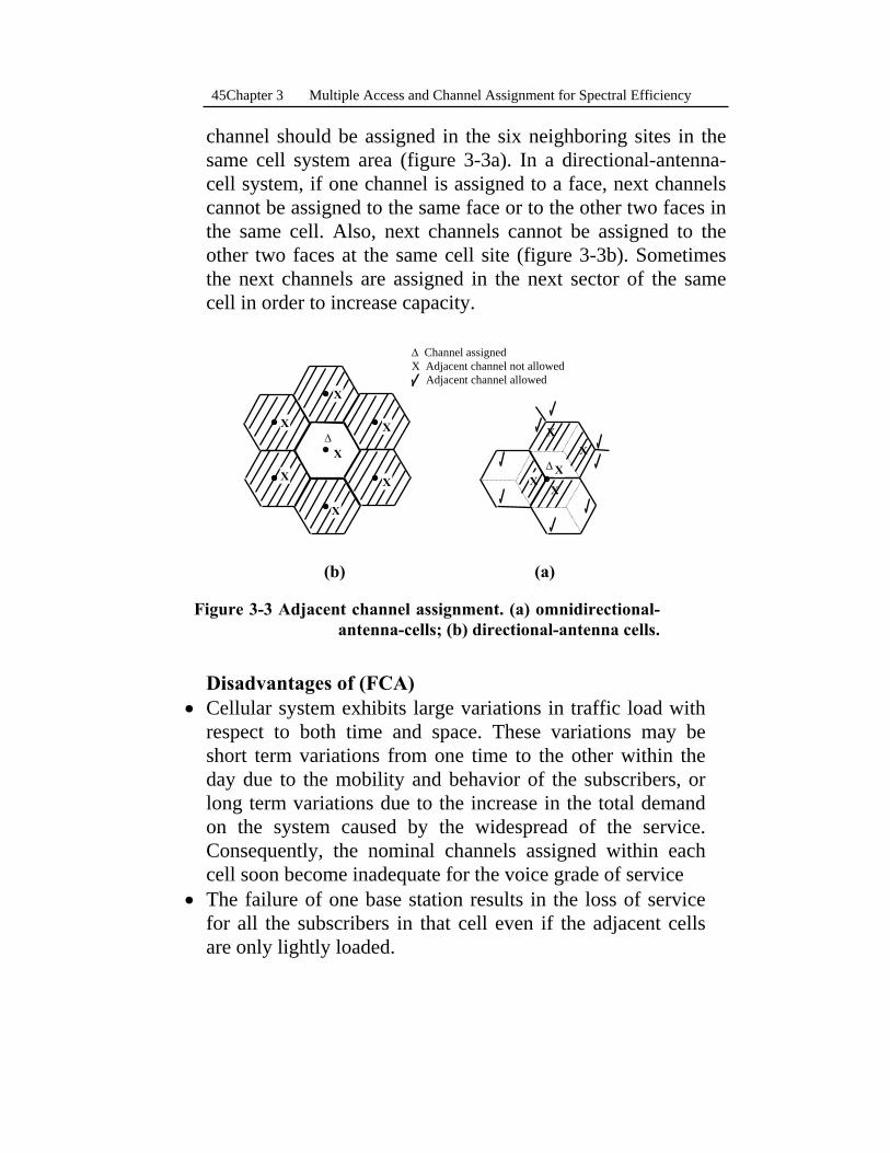
channel should be assigned in the six neighboring sites in the same cell system area (figure 3-3a). In a directional-antenna-cell system, if one channel is assigned to a face, next channels cannot be assigned to the same face or to the other two faces in the same cell. Also, next channels cannot be assigned to the other two faces at the same cell site (figure 3-3b). Sometimes the next channels are assigned in the next sector of the same cell in order to increase capacity. Disadvantages of (FCA)
• Cellular system exhibits large variations in traffic load with respect to both time and space. These variations may be short term variations from one time to the other within the day due to the mobility and behavior of the subscribers, or long term variations due to the increase in the total demand on the system caused by the widespread of the service. Consequently, the nominal channels assigned within each cell soon become inadequate for the voice grade of service
• The failure of one base station results in the loss of service for all the subscribers in that cell even if the adjacent cells are only lightly loaded.
X
ΔX X
X
X X
X
X
XX
XΔX
Δ Channel assigned X Adjacent channel not allowed Adjacent channel allowed
(a) (b)
Figure 3-3 Adjacent channel assignment. (a) omnidirectional-antenna-cells; (b) directional-antenna cells.
46 Multiple Access and Channel Assignment for Spectral Efficiency Chapter 3
3.2.2 Dynamic Channel Assignment (DCA) In contrast to FCA, in which the relationship between the cells and the channels is predetermined and invariant, Dynamic Channel Assignment (DCA) is characterized by the lack of a fixed relationship between cells and channels. DCA schemes relax the strict segmenting rules of the FCA which may lead to a call being blocked despite the existence of free channels in nearby cells. This relaxation attempts to allow nearby cells to share the available bandwidth in other cells. DCA is implemented by placing all of the available resources under the direct control of a central controller (e.g. MTSO). Channels are assigned spontaneously to calls upon requests.
It should be noted that the main point that characterizes a certain DCA scheme is the tie-breaking rule used to favor a certain channel. One approach for designing a tie-breaking rule is to aim at choosing a channel which has the least effect on adjacent cells in terms of blocking probability. Another approach is to choose a channel that minimizes the reuse distance of the channels according to the status of the network at the instant of the call request. Disadvantage of (DCA) The price paid is the increased complexity of the mobile unit and the requirement of global system information at call startup and at handoffs. This disadvantage is a considered one which dictates seeking for improvements to the FCA instead. 3.2.3 Improvements to (FCA) As discussed above, the FCA is the most common scheme because of its simplicity and its moderate requirements of centrally controlled operations. So, some improvements can be considered to avoid the short comings of this scheme while taking the advantage of the (DCA).
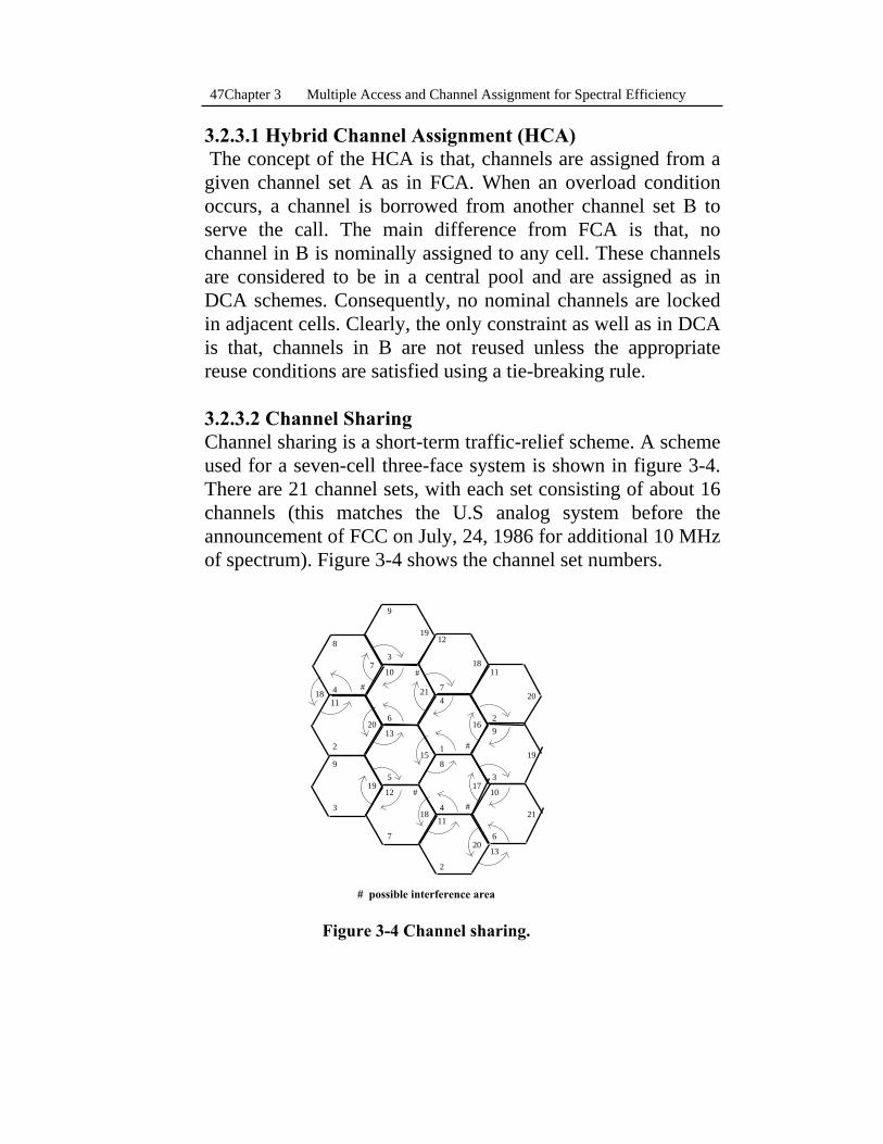
Chapter 3 Multiple Access and Channel Assignment for Spectral Efficiency 47
3.2.3.1 Hybrid Channel Assignment (HCA) The concept of the HCA is that, channels are assigned from a given channel set A as in FCA. When an overload condition occurs, a channel is borrowed from another channel set B to serve the call. The main difference from FCA is that, no channel in B is nominally assigned to any cell. These channels are considered to be in a central pool and are assigned as in DCA schemes. Consequently, no nominal channels are locked in adjacent cells. Clearly, the only constraint as well as in DCA is that, channels in B are not reused unless the appropriate reuse conditions are satisfied using a tie-breaking rule. 3.2.3.2 Channel Sharing Channel sharing is a short-term traffic-relief scheme. A scheme used for a seven-cell three-face system is shown in figure 3-4. There are 21 channel sets, with each set consisting of about 16 channels (this matches the U.S analog system before the announcement of FCC on July, 24, 1986 for additional 10 MHz of spectrum). Figure 3-4 shows the channel set numbers.
# possible interference area
Figure 3-4 Channel sharing.
8
9
1912
1811
20
2
4721
10
37
18114
916
13
620
21915
1
9
195
83
17
321
12 10
184
##
#
#
#
7
11
6
2
2013
48 Multiple Access and Channel Assignment for Spectral Efficiency Chapter 3
When a cell needs more channels, the channels of another face at the same cell site can be shared to handle the short-term overload. To obey the adjacent-channel assignment algorithm, the sharing is always cyclic. Sharing always increases the trunking efficiency of channels. Since we cannot allow adjacent channels to share with the nominal channels in the same cell, channel sets 4 and 5 cannot both be shared with channel sets 18 and 12 respectively, as indicated by the grid mark. Many grid marks are indicated in figure 3-4 for the same reason. However, the upper subset of set 4 can be shared with the lower subset of set 5 with no interference. 3.2.3.3 Static Channel Borrowing Static channel borrowing is handled on a long-term basis. The extent of borrowing more available channels from other cells depends on the traffic density in the area. Static channel borrowing can be implemented from one cell-site face to another face at the same cell site. In addition, the central cell site can borrow channels from neighboring cells. The channel-borrowing scheme is used primarily for slowly-growing systems. It is often helpful in delaying cell splitting in peak traffic areas. Since cell splitting is costly, it should be implemented only as last resort.
Once a static borrowing process has taken place, the allocation of channels to calls is exactly the same as in FCA. A call is rejected if none of the channels assigned the cell in which it originated is free. 3.2.3.4 Dynamic Channel Borrowing The main different point in this scheme from the static channel borrowing is that, it is performed on a call-by-call basis. That is, it is a short-term scheme not a long-term one.
Cells in peak traffic areas are allowed to borrow channels from less-loaded adjacent cells to handle excessive traffic. The borrowed channels will be used within the borrowing base
Chapter 3 Multiple Access and Channel Assignment for Spectral Efficiency 49
station. In the mean while, under normal traffic conditions, channels are allocated using the simple FCA scheme. When all nominal channels are occupied, borrowing of channels takes place.

Chapter 4
Introduction to Simulation
imulation as a technique or a set of techniques was probably known to most people before the late sixties when the space race and ,in particularly, the race to get to the
moon pushed it into prominence. Before that time, the only people who knew much about simulation were those actually used it to solve problems. It may be a coincidence, but also in the late sixties, a spate of definitions of simulation appeared in all the relevant literature. Many of the eminent simulationists of the time (McLeod, 1986, Gordon, 1996) gave their definitions, within which many common features emerged. A short definition for simulation was introduced, that is, “Simulation is an art whereby one could develop models to represent real or hypothetical systems”.
Simulation was also acknowledged to be a technique or a set of techniques whereby the development of models helps one to understand the behavior of a system, real or hypothetical. From this point of view we should introduce first a simple definition the system and a brief discussion about models.
4.1What Is a System? From the different interpretations that arose (Gordon, 1969, Shearer, Murphy and Richardson, 1967), a system could be considered to be a collection of objects, parts, components, call them what you will which interact with each other, within some notional boundary, to produce a particular pattern of behavior. The idea of a boundary was necessary to separate the system from the rest of the universe, to keep the task of studying its behavior within reasonable limits.
S
Chapter 4 Introduction to Simulation 51
4.2 What Is a Model? The logical development -as far as simulation is concerned-is to establish what constitutes a model, since the ‘art’ of simulation is essentially the modeling of systems, with the use of computers. In order to answer that question, we have to consider, very carefully, just what information we expect to obtain from the manipulation of a model during simulation studies. Once we have established that, even in general terms, then we can begin to decide what form our model should take. 4.3 Hierarchy of Models In the broadest sense, models take tow forms: physical (iconic or replica) models, or abstract (notional or mathematical) models. It is the abstract model that is more relevant to the idea of general-purpose simulation. However, it is useful in the wider context for us to consider and contrast both basic forms to see why this should be so. Figure 4-1 shows a simple tree structure displaying a hierarchy of general model structure. 4.3.1 Physical (Replica models) In the course of development work, many industries require the construction and testing of replica models for specific purposes. It uses to be the case that aircraft were the only form of transport subjected to wind tunnel testing during the course of design. This was to try to achieve an aerodynamic optimum in terms of low drag coefficients. Reducing drag reduced fuel consumption, which gave a better payload, and also probably reduced the required engine thrust needed to achieve a given airspeed. In other words, the economics of flight necessitated wind tunnel testing of replica models as part of the airframe design process.
But when we talk about simulation in our thesis we don’t concern, of course, the physical modeling. We just stated this type of modeling here to give a complete over view about modeling. So when we say ‘simulation’ hence and further we

52 Introduction to Simulation Chapter 4
are interested in simulation for the second type of modeling which is abstract models.
4.3.2 Abstract (Mathematical models) A notional or indeed mathematical model of a system is an abstraction of the reality it is meant to portray. By putting the ideas concerning the model of the real system - mathematical relationships or any other abstract form - an abstract model can take shape. It is quite clear that the ideas in the modeler’s mind concerning his perceptions about the way the real system should behave, will have considerable influence on the type of model that evolves.
4.3.2.1 Characteristics of Abstract Models. As seen from Figure 4-1, the abstract model could be discrete or continuous, equation oriented or block oriented, stochastic
Dynamic Static
Model
Continuous variable Discrete event
Block orientedEquation oriented
Deterministic Stochastic
AbstractPhysical
Figure 4-1 Hierarchy of model structure
Chapter 4 Introduction to Simulation 53
or deterministic, and finally static or dynamic. Each pair of features will be explained now to give a complete understanding to the abstract models. I) Discrete Event vs. Continuous Variable If model behavior changes continuously, such that model behavior characteristics should be accessible at every instant of time, then a continuous model results. If, on the other hand, the type of model is such that changes of state occur only at set instants of time, the model characteristics remaining constant at points in between, then a discrete model is required. This distinction is an example of the type of abstraction adopted, influencing the nature of the model that eventually takes shape.
By way of illustration, let us consider the modeling of a vehicular traffic flow situation. If the information demanded from the model is an average vehicle flow rate past a particular observation point, then a continuous model may be needed, especially if the information has to be produced in an unbroken form. Constant observation of the vehicle flow pattern is required, so every instant of time is equally important. If, however, it is specified that the model should give information about the individual arrival pattern of vehicles at the same observation point, then a discrete model may be more suitable. The only changes to the state of the model occur with each arrival at the observation point. Time is of no consequence in between each arrival. In practice, there is often a degree of overlap between the two model types, because of the nature of the real system behavior and the consequent information required from the model thereof. The modeling mix may be in any proportion deemed by the modeller to suit the task in hand.
II) Equation Oriented vs. Block Oriented The equation-oriented modeling form, facilitated by the use of modern high-level computer programming languages, preserves most of the identities of the mathematical
54 Introduction to Simulation Chapter 4
relationships embodied in the procedural coding statements, and quite complex modeling can be presented in one line of code.
The block oriented modeling is used to describe the in-hand system in terms of blocks, arrows, and input-output data. This technique was very familiar to simulationists who works on the analog computers, and that was because of the very nature of the analog computers which requires defining the model in a block-oriented way. The disadvantage of a purely block-based modeling approach is the need for very many blocks to represent the complexity present in a typical single-line mathematical relationship. Also departure from the form of the relationship can, for many, be accompanied by a loss of meaning upon dissection into many function blocks.
III) Stochastic vs. Deterministic If we consider the different systems we may be called upon to model, we would very soon come across uncertainty in various forms. We would most probably be uncertain about different aspects of the model structure itself, being unsure whether a particular relationship was the best way to describe some model feature. Even if we were sure about the model construction details, we would be uncertain about the authenticity, integrity and values of some of the data to be used in implementing simulation studies. In the simulation of engineering systems, we usually take a decision to ignore the uncertainties of model and data identification, and to treat the models as being deterministic. If the uncertainties are of little importance compared with the general dynamic behavior of the model, then such decisions are valid. If the uncertainties are sufficiently important to affect model dynamics, then they cannot be ignored.
When we consider the behavior of discrete systems and the corresponding models, a different picture emerges. Discrete modeling tends to involve the interaction of people with
Chapter 4 Introduction to Simulation 55
systems. Continuous models usually focus on the behavior of engineering systems, to the exclusion of the human factor. People inject a great deal of uncertainty into the behavior of any system with which they come into contact. They respond differently to a situation , react at different rates to an incident, and have a variety of ways in which they may interact with a system.
IV) Static vs. Dynamic A system could be static, that does not change its state with time, or dynamic that changes its state with time. Also the dynamic system has tow major states: the transient state and it starts by the first moment an input is applied to the system and lasts a period of time called the transient time. After that time the system enters its next state which is called steady state. But the thing we should focus on is steady state does not mean at all a static system. As an example, a simple RC circuit having a sinusoidal input voltage has a sinusoidal steady state current. 4.3.2.2 Abstract Models are Mixed From what stated above about model characteristic it should not be believed that there is a sever determinism in model or system type. That it is to say, systems or models of systems are very probably to be mixed from some contrasting pairs of features. We can find a model having almost deterministic parameters, but in the same time it has stochastic ones. Also a system could be described in a block oriented way but almost it will have some equations and continuous variable or parameters. But, generally speaking, we can say that, continuous models will almost be deterministic and discrete models will be stochastic.
Also dynamic models which feature sets of differential equations, either ordinary or partial, or indeed both kinds, will almost certainly be continuous models. The solution of differential equations does not come into discrete simulation
56 Introduction to Simulation Chapter 4
methodology. However, we can find such a system whose model constitutes from continuous and discrete parts. In the same way , we may look for the presence of sets of algebraic equations. Again a continuous model will probably contain many to define auxiliary system variables, whereas in discrete simulation there may be some algebraic relationships, but they will be few in relation to the size of the model.
If we look for the presence of what we may call logical relationships, or in other words, decision-making processes, we will find that in discrete models, decision-making is a very important feature, and the model operation is driven by the interaction of many such processes. Continuous models, on the other hand, may exhibit very little in the way of decision-making to alter the course of events as a simulation proceeds.
4.4 What Is Simulation? As stated in the very beginning of this chapter we had a short definition for simulation as defined in the first age of simulation. Also it is noticed that simulation for abstract models should be implemented on some computational device. It does not matter it the system whose model is in hand exists or not. We can now give a general definition for simulation as: “Computer simulation is the discipline of designing a model of an actual or theoretical physical system, executing the model on a computer, and analyzing the execution output”. 4.5 Why Simulate? There are many benefits for simulation which couldn’t be achieved neither by mathematical modeling nor by real life experimentation. In some situations these methods would suffice; however; simulation is able to tackle a wider range of issues.
Chapter 4 Introduction to Simulation 57
4.5.1 Simulation vs. Real Life Experimentation Experimentation can be performed by changing the inputs of the real life system and measuring the resulting change in behavior. For example, the number of operators at an inquiry center could be changed until a satisfactory service level is achieved. There are a number of reasons why simulation is preferable to this form of experimentation: I) Cost Real life experimentation can be very costly. It is certainly costly to employ and fire staff at will (if indeed it is possible) or to install additional equipment in order to measure the change in throughput. Having built a simulation model the only additional cost incurred is that of the man-time to change the model and perform the experiments. Ii) Repeatability Since the exact conditions of a real life experiment are unlikely to be repeated there is only one opportunity to collect the results. Further to this, there is no opportunity to compare the response to alternative inputs under these same conditions. By repeatedly generating the same sequence of events in a simulation model alternative scenarios can be tested under the same conditions. The arrival sequence of vehicles at a set of traffic lights could, for instance, be repeated to test the effect of alternative change frequencies for the lights. Results from different experiments could then be compared and the best scenario chosen. III) Control of the Time Base When carrying out a real life experiment with the production schedule for a manufacturing plant a month may be required to obtain a result for just one scenario. The same simulation experiment may take a matter of minute, enabling more scenarios to be examined in a much shorter time period,
58 Introduction to Simulation Chapter 4
increasing the possibility of finding a good solution. Sometimes increasing the run time is preferable, turning nanoseconds into seconds, especially when simulation electronic communications and computer networks. Simulation enables such control of the time base. IV) Legality and Safety Experimentation with new ideas in, say, a toxic chemical plant can be hazardous and even illegal. With simulation, ideas can be tested and once a solution has been found attention can be paid to the safety and legal requirements for implementation. 4.5.2 Simulation vs. Mathematical Modeling. There is an abundance of mathematical models that can be used successfully to represent real world systems, and implementing these models will in most cases be quicker than simulation. Examples of mathematical models are linear programming and queuing theory. Certainly, simulation should not be used when a simple ‘spreadsheet analysis’ will suffice. However, there are a number of good reasons why simulation should, in some circumstances, be used in preference to mathematical modeling: I) Dynamic and Transient Effects Frequently more information is required than just the ‘normal’ or ‘steady-state’ behavior of the system in question. For instance, when modeling a storage facility it is useful to understand the effects of major high bay crane breakdowns. It is the ability of simulation to cope with and provide results on these dynamic and transient effects that makes it more effective than mathematical tools. II) Non Standard Distributions Data may have been collected on, say, the service time at a supermarket. In queuing theory (as well as other mathematical
Chapter 4 Introduction to Simulation 59
models) the modeller is restricted to a set of standard service time distributions and so an approximation may have to be made. However, a simulation model can include both standard distributions and distributions based on collected data, enabling the modeller to avoid unnecessary simplification. III) Interaction of Random Events When a machine breaks down on a production line the stoppage will have significant ‘knock-on’ effects. Mathematical models cannot easily represent the complex interaction caused by such random events. In general, as the number of random variables increases there is a more proportional increase in complexity. Simulation is able to handle these complex interactions and predict their effect. 4.5.3 Benefits from Applying Simulation As a result of the above benefits of simulation over the mathematical modeling or life experiments, we have an ultimate benefits gained from applying simulation there are:
• Greater understanding for the physical system. • Enhancing Engineering design for practical systems. • Risk reduction. • Lead time reduction. • Faster system development. • Improved customer service.
4.6 Simulation Software For the implementation of a simulation model on a digital computer some software development is necessary. There are three categories for simulation software, we will discuss them and illustrate the main features of each one. Table 4-1 illustrates the main differences among the three types of simulation software.
60 Introduction to Simulation Chapter 4
4.6.1 User-Built Programs They are user defined or built. More obviously, the simulationist himself who writes the source code of the simulation program by using any programming language. Some libraries having certain functions specially for simulation purposes are written either by the company whose compiler is used or by other teams dedicated for that purpose, or some are developed by the programmer-simulationist- himself. But the thing to say here, this type of simulation software with respect to simulation somehow looks like assembly language with respect to programming. We mean it is so primitive and many functions -or even complete modules- will be needed to be used in the source code. Also, getting into very details makes it very probable to make mistakes. So this type of simulation software needs a professional programmer. But an ultimate benefit and a supreme gain from this user-built-programs is mastering the simulation. That is because, getting deeply in the details -as the nature of writing source code- ,building new functions and compilation errors makes one very familiar with the problem he simulates. 4.6.2 Simulation Languages Simulation languages are general in nature but may have special features for certain types of application such as networking and manufacturing . A model is developed by writing a program using the constructs of the language. 4.6.3 Simulators Simulators are packages that model a specific class of application. They are generally menu driven , requiring a user to input data and basic logic commands while little or no programming skills are required. At one extreme, some simulators are very flexible, enabling them to be used on a wide range of applications. Some are able to interface with
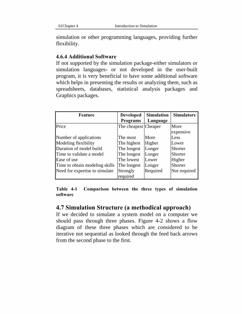
Chapter 4 Introduction to Simulation 61
simulation or other programming languages, providing further flexibility. 4.6.4 Additional Software If not supported by the simulation package-either simulators or simulation languages- or not developed in the user-built program, it is very beneficial to have some additional software which helps in presenting the results or analyzing them, such as spreadsheets, databases, statistical analysis packages and Graphics packages.
Feature Developed Programs
Simulation Language
Simulators
Price The cheapest Cheaper More expensive
Number of applications The most More Less Modeling flexibility The highest Higher Lower Duration of model build The longest Longer Shorter Time to validate a model The longest Longer Shorter Ease of use The lowest Lower Higher Time to obtain modeling skills The longest Longer Shorter Need for expertise to simulate Strongly
required Required Not required
Table 4-1 Comparison between the three types of simulation software
4.7 Simulation Structure (a methodical approach) If we decided to simulate a system model on a computer we should pass through three phases. Figure 4-2 shows a flow diagram of these three phases which are considered to be iterative not sequential as looked through the feed back arrows from the second phase to the first.
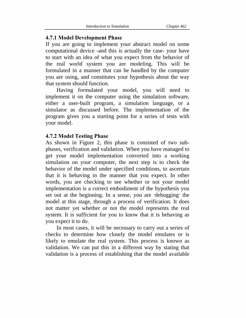
62 Introduction to Simulation Chapter 4
4.7.1 Model Development Phase If you are going to implement your abstract model on some computational device -and this is actually the case- your have to start with an idea of what you expect from the behavior of the real world system you are modeling. This will be formulated in a manner that can be handled by the computer you are using, and constitutes your hypothesis about the way that system should function.
Having formulated your model, you will need to implement it on the computer using the simulation software, either a user-built program, a simulation language, or a simulator as discussed before. The implementation of the program gives you a starting point for a series of tests with your model. 4.7.2 Model Testing Phase As shown in Figure 2, this phase is consisted of two sub-phases, verification and validation. When you have managed to get your model implementation converted into a working simulation on your computer, the next step is to check the behavior of the model under specified conditions, to ascertain that it is behaving in the manner that you expect. In other words, you are checking to see whether or not your model implementation is a correct embodiment of the hypothesis you set out at the beginning. In a sense, you are ‘debugging’ the model at this stage, through a process of verification. It does not matter yet whether or not the model represents the real system. It is sufficient for you to know that it is behaving as you expect it to do.
In most cases, it will be necessary to carry out a series of checks to determine how closely the model emulates or is likely to emulate the real system. This process is known as validation. We can put this in a different way by stating that validation is a process of establishing that the model available

Chapter 4 Introduction to Simulation 63
is a sufficiently correct model of the real system. This is one of the most difficult area of simulation study.
There are two different aspects from which to view the problem of validation. The first is the case where validation is required for a simulation model of an existing system. The second, but more difficult, problem is validation of a model for a hypothetical or projected system.
In case of existing system, difficulties are represented in running the simulation program many times at the same operating conditions of the real system, then comparing the simulation results with the real system behavior. But when it comes to validate a model for hypothetical system the task will be more difficult because of missing the real-life behavior to compare with.
4.7.3 Exploiting Phase This phase is concerned with the practical achievement of the simulated system. Although we are not interested in this phase
Figure 4-2 Flow diagram for simulation phases
Development PhaseFormulation
Programming
Exploitation Phase
Experimentation
Implementation
Testing Phase
Verification
Validation

64 Introduction to Simulation Chapter 4
in our thesis -because of it is considered to be out of research problems- we must just touch it to make a complete over view for the three phases of a complete simulation task. Let us assume that we have obtained a working simulation, and that we have validated the model and shown that its operation is a true and correct representation of that of the real system. Nevertheless, we should ensure that the real life system will respond in the same way that indicated by the simulation results, specially if the simulation was for a hypothetical system. This is called experimentation, and it is a sub-phase of the exploitation phase.
Having finished from the experimentation sub-phase, and got satisfied and sure about the would-be system performance, the last stage comes into consideration which is the final implementation of the system, in which the real physical system is built. 4.8 A Short History of Simulation Evolution We will discuss in this section very briefly the evolution of simulation since it started until the day on.
When simulation came into the scientific world at its first time it was carried on the analog computers. Simulation on analog computers is by building hardware -electronic circuits- each circuit simulates one part or module of the whole system. Then by measuring and testing the voltages and currents at specific nodes and branches, simulationists get information about the behavior of the simulated model.
Early analog computers were notoriously unreliable machines, particularly so when you consider that the electronics was based on very old-fashioned valve (vacuum-tube) technology. Maintaining hundreds of DC amplifiers in working order, for the implementation of even a medium-sized model, was a full-time job, and one could never be absolutely sure about the results. The larger the model, the greater the

Chapter 4 Introduction to Simulation 65
number of analog components required, with a corresponding increase in overall unreliability.
The one great redeeming feature of the analog computer as far as continuous simulation was concerned, was the ability to carry out the operation of integration very quickly indeed, and at a rate independent of the size of the model. This meant that differential equation should be solved at very high speed, useful for carrying out any hundreds of simulation runs in a short space of time.
When coming , after, to the age of digital computers, early digital computer were not much better for the same reason of hardware complexity and its unwelcome large number of vacuum tubes. Coupled with that reason, comes to consideration the fact that programming was a nightmare. Until that time the analog computer had the speed advantage over digital one. But the advance of transistor technology, followed by integrated circuitry, meant that both digital and analog computer hardware became much more reliable. The increase in solution speed obtained with every advance in digital hardware technology whittled away the speed advantage obtained from the analog computer.
Apart from the hardware advances, ease of programming or implementing a model on the relevant computer hardware had to be taken into consideration. Analog computers were never the easiest devices to program. Problem preparation in the way of scaling and circuit design could lead to many implementation errors that were not always easy to trace. Digital processors, on the other hand, with high-level programming languages, good operating systems, and helpful utilities for program debugging, became relatively easy to program , and setting up a simulation model developed into a somewhat easier task on a digital machine.
After development of digital computers, the hybrid computers came into the computer world. They enjoyed a
66 Introduction to Simulation Chapter 4
relatively brief period of popularity but has since almost vanished. The rationale behind the development of the hybrid was the desire to have the best of both worlds in combining analog and digital computers together into one machine, each communicating with the other through an interface. Several advantages were gained from this combination, most of all in the use of digital software to assist in programming and setting up the analog machine. However, the complexities of model implementation and debugging brought about the demise of the hybrid in favor of a wholly digital approach.
As far as discrete simulation was concerned, there was
never a conflict of interests for hardware implementations. Operational research as a management science tool only
Figure 4-3 Simulation and different types of computers and simulation software
User-built Programs
Continuous-variable models
Discrete-event models
Hybrid Computer Analog ComputerDigital Computer
Simulation Language
Simulators
Simulated on Simulated on
Software used Software used
Chapter 4 Introduction to Simulation 67
developed when digital computer hardware was well advanced and good-quality mainframe machines were available. This historical timing, together with the fact that discrete models are best suited to digital implementation, meant that analog machinery has hardly ever been used. Figure 4-3 shows the relation among simulation, computer types, and software simulations types. 4.9 Simulation Tool in this Thesis As illustrated in Table 4-1, each of the three types of simulation software has advantages and disadvantages. So if we have a simulation tool that combines the privileges of the two extreme software, the Developed Programs and Simulators, it will be the best choice. Fortunately, OPNET/MODELER simulation package is a comprehensive software environment for modeling, simulation, and analyzing the performance of communications networks, computer systems and applications, and distributed system.
To provide useful data and flexible simulation, network models must combine accurate descriptions of topology, data flow, and control flow. since no single paradigm of visual representation is ideally suited for all three of these model types, OPNET utilizes separate model formats for each. To lend structure and discipline to the overall model, OPNET models fit together in a hierarchical fashion:
4.9.1 Modeling Networks The OPNET network editor graphically captures the physical topology of a communication network. Networks consist of node and link objects, which are graphically assembled and parameterized via pop-up dialog boxes. To create node objects, users select node types from a library of example and user-defined models. Each OPNET node model has a specific set of attributes that are used to configure it. Networks models can be constructed in a dimensioned work space with a user-selected
68 Introduction to Simulation Chapter 4
grid. Since users may define node abstractions, OPNET network models may represent LAN’s, MAN’s, WAN’s, on-board vehicular networks, or any combination thereof. Subnetwork objects can be used to structure an unlimited topology hierarchy within any network model. Users can load a customized cartographic background to define a physical context for wide-area networks. 4.9.2 Modeling Nodes The OPNET node editor graphically captures node architectures, which are diagrams of data flow between modules typically representing hardware and software subsystems. Module types include processors, queues, traffic generators, receivers, and transmitters. Processors are general modules that provide complete flexibility in protocol and algorithm specification. The functionality of processor and queue objects is defined using OPNET process model. Instances of OPNET node models are used to populate OPNET network models. 4.9.3 Modeling Processes The OPNET process editor uses a powerful state-transition diagram approach to support specification of any type of protocol, resource, application, algorithm, or queuing policy. States and transitions graphically define the progression of a process in response to simulated events. Within each state, general logic can be specified using a library of over 350 pre-defined functions. The full flexibility of the C programming language is also accessible. As with other OPNET editors, users can construct entirely new process models, or modify those provided with the environment.
Once a set of OPNET network, node, and process models are fully defined, users can run simulation studies based on them via the OPNET simulation tool. Users can see dynamic model behavior (at all three levels) in the OPNET animation

Chapter 4 Introduction to Simulation 69
viewer, and plot statistical performance measurements based on simulation studies in the OPNET analysis tool. 4.9.4 Analyzing OPNET Simulation Results The OPNET analysis tool provides a graphical environment that allows users to view and manipulate data collected during simulation runs. Standard and user-specified probes can be inserted at any point in a model to collect statistics. Simulation output collected by probes can be displayed graphically, viewed numerically, or exported to other software packages. First and second order statistics on each trace as well as confidence intervals can be automatically calculated. OPNETG supports the display of data traces as time-series plots, histograms, probability density and cumulative distribution functions, and scattergrams. Graphs (as with models at any level in the OPNET modeling hierarchy) may be output to a printer or saved as bitmap files to included in reports or proposals.
Chapter 5
Simulation and Analysis for a Preemptive Priority Model
his chapter is dedicated to analyzing a preemptive priority model proposed in the literature first in [10], then revised later in [17]. This model handles the special case of having
a cellular system which supports only two types of services, voice calls and data packets while having a preemptive priority for the voice calls over the data packets as will be explained later in this chapter. When proposed first in [10], only the set of equations were derived but neither these equations were solved nor the system performance was analyzed. Later, this work was revised in [17] by finding out and correcting some vital mathematical mistakes, then completed by solving the system numerically and illustrating the system performance by plotting the different measurement parameters for both, the voice calls and data packets.
After a careful study for the above work, two mathematical modifications are introduced, the matter that changed the system performance noticeably. Having considered the mathematical modifications, a numerical solution for the mathematical model was carried out using MATHEMATICA Software and measurement parameters were plotted. On the other hand, simulation was run on the OPNET/MODELER simulation environment and measurement parameters were plotted also. The results obtained from these two different techniques are shown to be in a complete matching with each other. Also the model was resolved numerically again but without considering the modifications, this led to the same results obtained in [17], while obvious discrepancies are found between these results on a hand and the
T

Chapter 5 Simulation and Analysis for a Preemptive Priority Model 71
results obtained from numerical solution and simulation after considering the modifications on the other hand.
In this chapter the model’s equations will be derived. The measurement parameters will be introduced in their final form -after modifications done by [17] - without mentioning them. Then, our comments on this work will be explained and the two mathematical modifications will be introduced and derived. Finally, the results obtained from simulation, numerical solution after modifications, and numerical solution before modifications will be compared. 5.1 System Description The system is considered to have C available channels and a finite queue length of K-C to have a total system capacity of K. Both, the voice calls and the data packets, are assigned channels directly as long as free channels are available (that is the total number of users-in-serves is less than C). Data packets will join the queue in the case of not having free channels. Consequently, data packets will be blocked if the queue is full. However, the policy is different for the voice calls which will join the queue if and only if all the C channels are accessed only by voice calls. If the C channels are full of the two types of traffic, the first coming voice call will dismiss a data packet from a channel, replace it, and force it to join the queue if it is not full or it will be dismissed from the whole system. The same policy will occur if the system is full while a voice call requests a service. In this case -of course the C channels are busy with voice calls- the voice call will dismiss a data packet from the queue, consequently from the system, and replace it. This policy is called the preemptive priority for voice calls over the data packets. Moreover, the voice calls are given the head-of-the-line priority (HOL) within the queue. The detailed description for the algorithm is indicated in figure
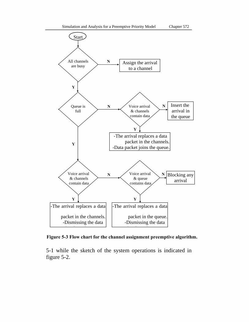
72 Simulation and Analysis for a Preemptive Priority Model Chapter 5
5-1 while the sketch of the system operations is indicated in figure 5-2.
Voice arrival & channels contain data
Voice arrival & queue
contains data
Voice arrival & channels contain data
Insert the arrival in the queue
Blocking any arrival
-The arrival replaces a data
packet in the queue. -Dismissing the data
k f h
-The arrival replaces a data
packet in the channels. -Dismissing the data
k f h
-The arrival replaces a data packet in the channels.
-Data packet joins the queue.
Assign the arrival to a channel
All channelsare busy
Queue is full
Y
Y
N
N
N
N
Y
Y
Y
N
Figure 5-3 Flow chart for the channel assignment preemptive algorithm.
Start
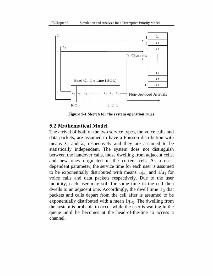
Chapter 5 Simulation and Analysis for a Preemptive Priority Model 73
5.2 Mathematical Model The arrival of both of the two service types, the voice calls and data packets, are assumed to have a Poisson distribution with means λ1 and λ2 respectively and they are assumed to be statistically independent. The system does not distinguish between the handover calls, those dwelling from adjacent cells, and new ones originated in the current cell. As a user-dependent parameter, the service time for each user is assumed to be exponentially distributed with means 1/μ1 and 1/μ2 for voice calls and data packets respectively. Due to the user mobility, each user may still for some time in the cell then dwells to an adjacent one. Accordingly, the dwell time TQ that packets and calls depart from the cell after is assumed to be exponentially distributed with a mean 1/μQ. The dwelling from the system is probable to occur while the user is waiting in the queue until he becomes at the head-of-the-line to access a channel.
To Channels
Head Of The Line (HOL)
Non-Serviced Arrivals
λ1
λ2
123
C
λ1
λ1
λ1
λ1
λ1
λ1
λ1λ2 λ2 λ2 λ1 λ1 λ1
K-C 3 2 1
Figure 5-1 Sketch for the system operation rules
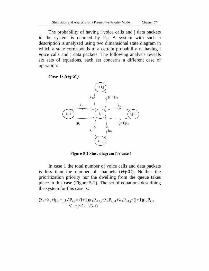
74 Simulation and Analysis for a Preemptive Priority Model Chapter 5
The probability of having i voice calls and j data packets in the system is denoted by Pi,j. A system with such a description is analyzed using two dimensional state diagram in which a state corresponds to a certain probability of having i voice calls and j data packets. The following analysis reveals six sets of equations, each set concerns a different case of operation.
Case 1: (i+j<C)
In case 1 the total number of voice calls and data packets
is less than the number of channels (i+j<C). Neither the prioritization priority nor the dwelling from the queue takes place in this case (Figure 5-2). The set of equations describing the system for this case is:
(λ1+λ2+iμ1+jμ2)Pi,j = (i+1)μ1Pi+1,j+λ2Pi,j-1+λ1Pi-1,j+(j+1)μ2Pi,j+1
∀ i+j<C (5-1)
i+1,j
λ2
(j+1)μ2
λ2
jμ2
iμ1 λ1
(i+1)μ1 λ1
i,j i,j+1 i,j-1
i-1,j
Figure 5-2 State diagram for case 1
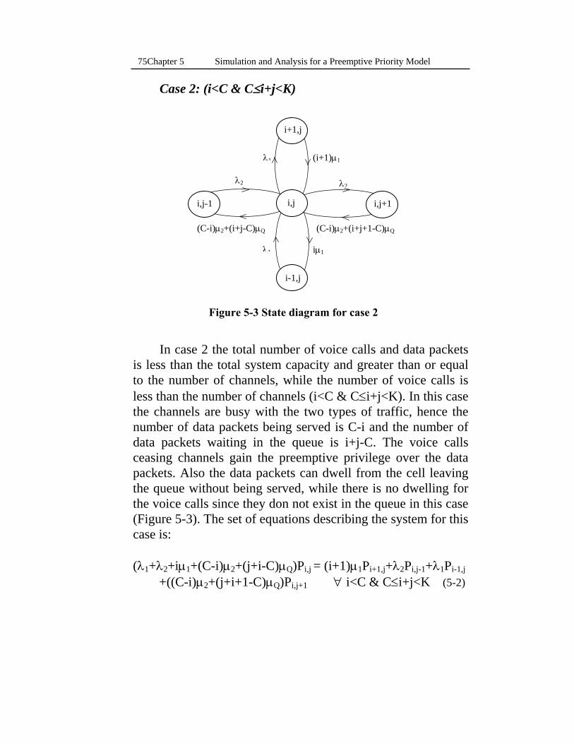
Chapter 5 Simulation and Analysis for a Preemptive Priority Model 75
Case 2: (i<C & C≤i+j<K)
In case 2 the total number of voice calls and data packets
is less than the total system capacity and greater than or equal to the number of channels, while the number of voice calls is less than the number of channels (i<C & C≤i+j<K). In this case the channels are busy with the two types of traffic, hence the number of data packets being served is C-i and the number of data packets waiting in the queue is i+j-C. The voice calls ceasing channels gain the preemptive privilege over the data packets. Also the data packets can dwell from the cell leaving the queue without being served, while there is no dwelling for the voice calls since they don not exist in the queue in this case (Figure 5-3). The set of equations describing the system for this case is: (λ1+λ2+iμ1+(C-i)μ2+(j+i-C)μQ)Pi,j = (i+1)μ1Pi+1,j+λ2Pi,j-1+λ1Pi-1,j +((C-i)μ2+(j+i+1-C)μQ)Pi,j+1 ∀ i<C & C≤i+j<K (5-2)
i+1,j
λ2
(C-i)μ2+(i+j+1-C)μQ
λ2
(C-i)μ2+(i+j-C)μQ
iμ1 λ1
(i+1)μ1 λ1
i,j i,j+1 i,j-1
i-1,j
Figure 5-3 State diagram for case 2
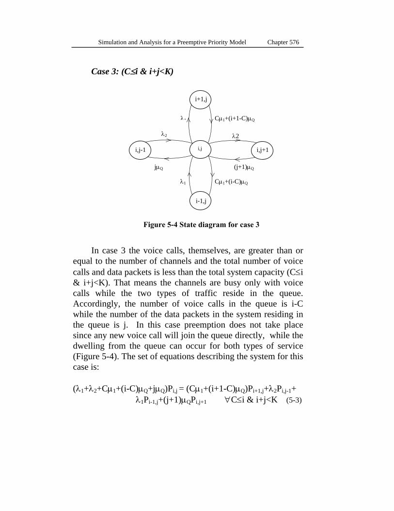
76 Simulation and Analysis for a Preemptive Priority Model Chapter 5
Case 3: (C≤i & i+j<K)
In case 3 the voice calls, themselves, are greater than or
equal to the number of channels and the total number of voice calls and data packets is less than the total system capacity (C≤i & i+j<K). That means the channels are busy only with voice calls while the two types of traffic reside in the queue. Accordingly, the number of voice calls in the queue is i-C while the number of the data packets in the system residing in the queue is j. In this case preemption does not take place since any new voice call will join the queue directly, while the dwelling from the queue can occur for both types of service (Figure 5-4). The set of equations describing the system for this case is:
(λ1+λ2+Cμ1+(i-C)μQ+jμQ)Pi,j = (Cμ1+(i+1-C)μQ)Pi+1,j+λ2Pi,j-1+ λ1Pi-1,j+(j+1)μQPi,j+1 ∀C≤i & i+j<K (5-3)
i+1,j
λ2
(j+1)μQ
λ2
jμQ
Cμ1+(i-C)μQ λ1
Cμ1+(i+1-C)μQ λ1
i,j i,j+1 i,j-1
i-1,j
Figure 5-4 State diagram for case 3
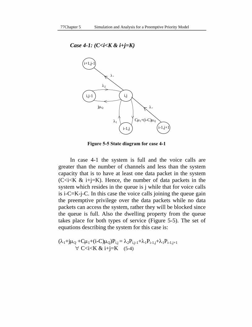
Chapter 5 Simulation and Analysis for a Preemptive Priority Model 77
Case 4-1: (C<i<K & i+j=K)
In case 4-1 the system is full and the voice calls are
greater than the number of channels and less than the system capacity that is to have at least one data packet in the system (C<i<K & i+j=K). Hence, the number of data packets in the system which resides in the queue is j while that for voice calls is i-C=K-j-C. In this case the voice calls joining the queue gain the preemptive privilege over the data packets while no data packets can access the system, rather they will be blocked since the queue is full. Also the dwelling property from the queue takes place for both types of service (Figure 5-5). The set of equations describing the system for this case is: (λ1+jμQ +Cμ1+(i-C)μQ)Pi,j = λ2Pi,j-1+λ1Pi-1,j+λ1Pi-1,j+1 ∀ C<i<K & i+j=K (5-4)
Figure 5-5 State diagram for case 4-1
i+1,j-1
λ2
jμQ
Cμ1+(i-C)μQ λ1
λ1
λ1
i,j
i-1,j+1
i,j-1
i-1,j
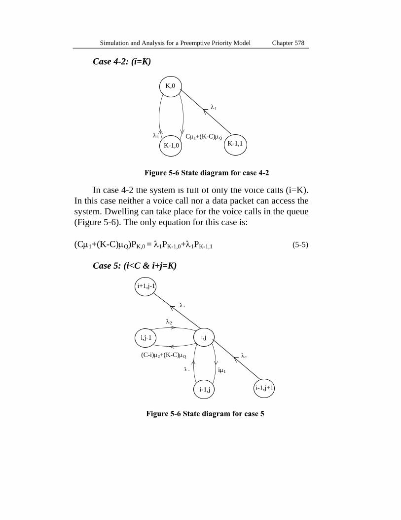
78 Simulation and Analysis for a Preemptive Priority Model Chapter 5
Case 4-2: (i=K)
In case 4-2 the system is full of only the voice calls (i=K).
In this case neither a voice call nor a data packet can access the system. Dwelling can take place for the voice calls in the queue (Figure 5-6). The only equation for this case is:
(Cμ1+(K-C)μQ)PK,0 = λ1PK-1,0+λ1PK-1,1 (5-5)
Case 5: (i<C & i+j=K)
Figure 5-6 State diagram for case 5
i+1,j-1
λ2
(C-i)μ2+(K-C)μQ
iμ1 λ1
λ1
λ1
i,j
i-1,j+1
i,j-1
i-1,j
λ1
Figure 5-6 State diagram for case 4-2
Cμ1+(K-C)μQ
λ1
K,0
K-1,1 K-1,0
Chapter 5 Simulation and Analysis for a Preemptive Priority Model 79
In case 5 the system is full and the number of voice calls is less than the number of channels (i<C & i+j=K). So, the number of the data packets in the queue is i+j-C=K-C. In this case the data packets are not permitted to access the system since it is full, while the voice calls have the preemption over the data packets in the channels. Hence, the voice calls can dismiss data packets from channels, consequently from the system. Also, dwelling is probable for only the data packets since there are no voice calls in the queue (Figure 5-6). The set of equations describing the system for this case is:
(λ1+(C-i)μ2+(K-C)μQ+iμ1)Pi,j = λ2Pi,j-1+λ1Pi-1,j +λ1Pi-1,j+1 ∀ i<C & i+j=K (5-6)
The two dimensional work-space for the data packets and the voice calls is represented in figure 5-7. Each case we derived had a certain condition for the data packets and the voice calls. Each condition is represented on the figure as a two dimensional region. From the figure it is obvious that the total number of unknowns is given by: No. of Unknowns = (1+2+3+…+(K+1)) = (K+1)(K+3)/2 (5-7)
The number of equations derived is less than the number of unknowns by only one equation which is the dependent equation. The dependent equation shown in figure 5-7 is that one which can be derived from all other equations. Alternatively, if we derived that equation as done in equation (5-5) it will not contribute to the system of equations since it can be derived explicitly from the others, the matter which would lead to a system of equations having a coefficient matrix whose determinant is zero. Of course the remaining equation is to force the summation of all the probabilities to be one:
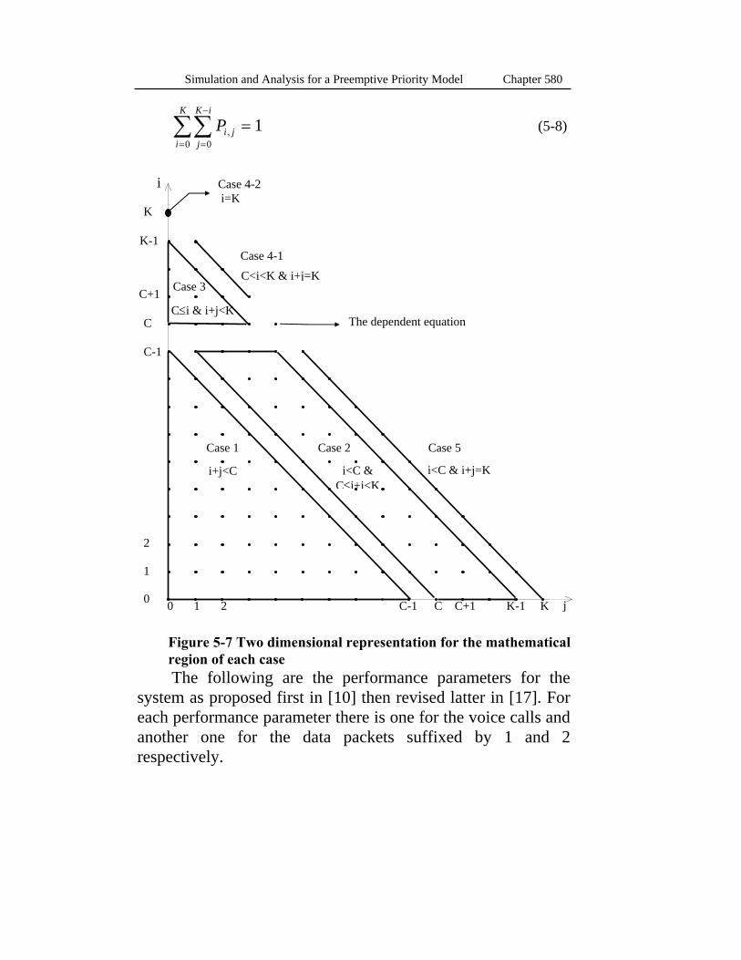
80 Simulation and Analysis for a Preemptive Priority Model Chapter 5
Pi jj
K i
i
K
,=
−
=∑∑ =
00
1 (5-8)
The following are the performance parameters for the system as proposed first in [10] then revised latter in [17]. For each performance parameter there is one for the voice calls and another one for the data packets suffixed by 1 and 2 respectively.
Case 3
Case 4-1
Case 5 Case 2 Case 1
i
j K-1 C+1 C-1 0 1 2 C K
K-1
C+1
C-1
0
1
2
C
K
The dependent equation
C<i<K & i+j=K
C≤i & i+j<K
i<C & i+j=K i<C & C≤i+j<K
i+j<C
Case 4-2 i=K
Figure 5-7 Two dimensional representation for the mathematical region of each case
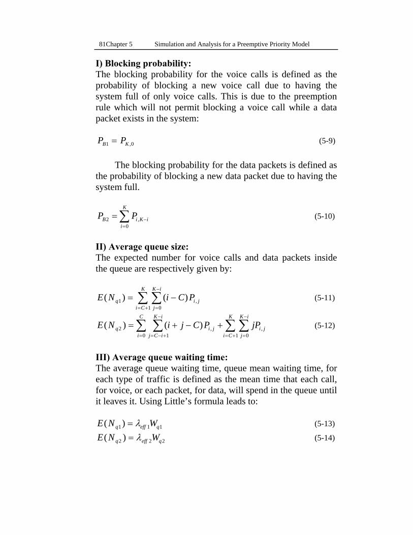
Chapter 5 Simulation and Analysis for a Preemptive Priority Model 81
I) Blocking probability: The blocking probability for the voice calls is defined as the probability of blocking a new voice call due to having the system full of only voice calls. This is due to the preemption rule which will not permit blocking a voice call while a data packet exists in the system:
P PB K1 0= , (5-9)
The blocking probability for the data packets is defined as
the probability of blocking a new data packet due to having the system full.
P PB i K ii
K
20
= −=∑ , (5-10)
II) Average queue size: The expected number for voice calls and data packets inside the queue are respectively given by:
E N i C Pq i jj
K i
i C
K
( ) ( ) ,101
= −=
−
= +∑∑ (5-11)
E N i j C P jPq i jj C i
K i
i
C
i jj
K i
i C
K
( ) ( ) , ,210 01
= + − += − +
−
= =
−
= +∑∑ ∑∑ (5-12)
III) Average queue waiting time: The average queue waiting time, queue mean waiting time, for each type of traffic is defined as the mean time that each call, for voice, or each packet, for data, will spend in the queue until it leaves it. Using Little’s formula leads to:
E N Wq eff q( )1 1 1= λ (5-13) E N Wq eff q( )2 2 2= λ (5-14)

82 Simulation and Analysis for a Preemptive Priority Model Chapter 5
where λeff1 & λeff2 are the actual rates for entering the queue for the voice and data respectively. Hence they are given by: λ λeff BP1 1 11= −( ) (5-15) λ λeff BP2 2 21= −( ) (5-16)
IV) Failure probability: The failure probability for any type of services is defined as the probability of leaving the cell, while being waiting in the queue due to the mobility, without getting a service. That is to fail to cease a channel. This parameter was proposed in [10] as:
P P PF i ji C
K
Q1 1==∑ , (5-17)
P P PF i jj C i
K i
i
K
Q210
2== − +
−
=∑∑ , (5-18)
Where PQ1 & PQ2 are the probabilities of having the average dwell time greater than the queue average waiting time, mean waiting time, for the voice calls and data packets respectively. They were derived in [10] assuming that the waiting time in the queue follows an exponential distribution with means 1/w1 & 1/w2 for voice calls and data packets respectively. The derivation for these two values yielded to:
PwQ
Q
Q1
1
=+
μμ
(5-19)
PwQ
Q
Q2
2
=+
μμ
(5-20)
Obviously, w1 & w2 should be substituted by 1/Wq1 & 1/Wq2 from equations 5-13 and 5-14 respectively.
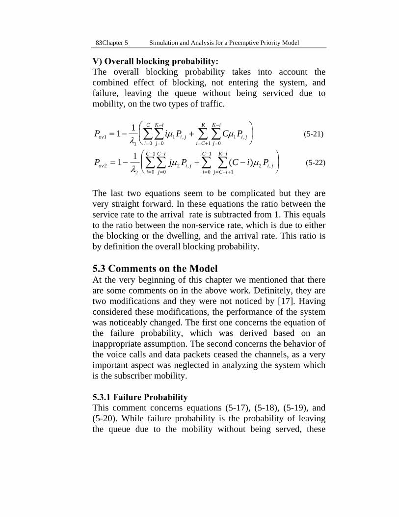
Chapter 5 Simulation and Analysis for a Preemptive Priority Model 83
V) Overall blocking probability: The overall blocking probability takes into account the combined effect of blocking, not entering the system, and failure, leaving the queue without being serviced due to mobility, on the two types of traffic.
P i P C Pov i jj
K i
i jj
K i
i C
K
i
C
11
10
1010
1 1= − +
⎛
⎝⎜
⎞
⎠⎟
=
−
=
−
= +=∑ ∑∑∑λ
μ μ, , (5-21)
P j P C i Pov i jj
C i
i jj C i
K i
i
C
i
C
22
20
210
1
0
1
11
= − + −⎛
⎝⎜
⎞
⎠⎟
=
−
= − +
−
=
−
=
−
∑ ∑∑∑λμ μ, ,( ) (5-22)
The last two equations seem to be complicated but they are very straight forward. In these equations the ratio between the service rate to the arrival rate is subtracted from 1. This equals to the ratio between the non-service rate, which is due to either the blocking or the dwelling, and the arrival rate. This ratio is by definition the overall blocking probability. 5.3 Comments on the Model At the very beginning of this chapter we mentioned that there are some comments on in the above work. Definitely, they are two modifications and they were not noticed by [17]. Having considered these modifications, the performance of the system was noticeably changed. The first one concerns the equation of the failure probability, which was derived based on an inappropriate assumption. The second concerns the behavior of the voice calls and data packets ceased the channels, as a very important aspect was neglected in analyzing the system which is the subscriber mobility. 5.3.1 Failure Probability This comment concerns equations (5-17), (5-18), (5-19), and (5-20). While failure probability is the probability of leaving the queue due to the mobility without being served, these
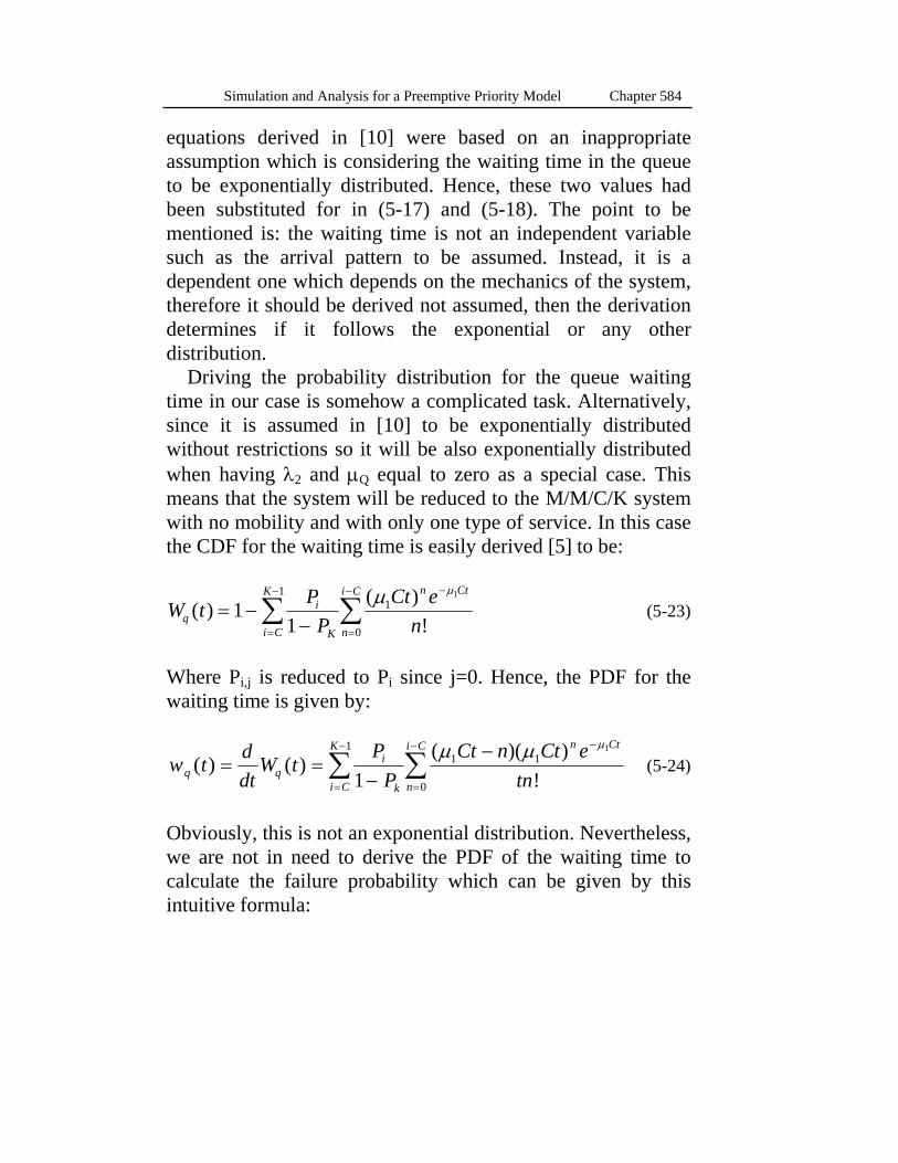
84 Simulation and Analysis for a Preemptive Priority Model Chapter 5
equations derived in [10] were based on an inappropriate assumption which is considering the waiting time in the queue to be exponentially distributed. Hence, these two values had been substituted for in (5-17) and (5-18). The point to be mentioned is: the waiting time is not an independent variable such as the arrival pattern to be assumed. Instead, it is a dependent one which depends on the mechanics of the system, therefore it should be derived not assumed, then the derivation determines if it follows the exponential or any other distribution.
Driving the probability distribution for the queue waiting time in our case is somehow a complicated task. Alternatively, since it is assumed in [10] to be exponentially distributed without restrictions so it will be also exponentially distributed when having λ2 and μQ equal to zero as a special case. This means that the system will be reduced to the M/M/C/K system with no mobility and with only one type of service. In this case the CDF for the waiting time is easily derived [5] to be:
W tP
PCt e
nqi
Ki C
K n Ct
n
i C
( )( )
!= −
−=
− −
=
−
∑ ∑11
11
0
1μ μ
(5-23)
Where Pi,j is reduced to Pi since j=0. Hence, the PDF for the waiting time is given by:
w t ddt
W tP
PCt n Ct e
tnq qi
ki C
K n Ct
n
i C
( ) ( )( )( )
!= =
−−
=
− −
=
−
∑ ∑1
11 1
0
1μ μ μ
(5-24)
Obviously, this is not an exponential distribution. Nevertheless, we are not in need to derive the PDF of the waiting time to calculate the failure probability which can be given by this intuitive formula:
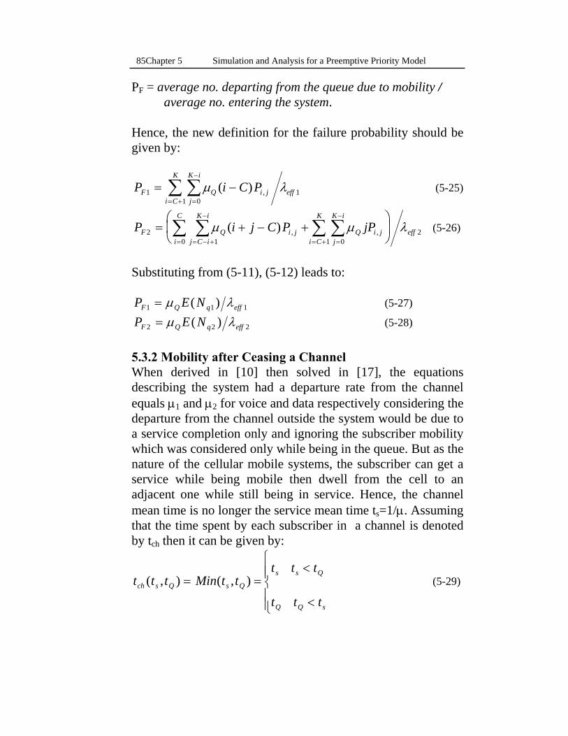
Chapter 5 Simulation and Analysis for a Preemptive Priority Model 85
PF = average no. departing from the queue due to mobility / average no. entering the system. Hence, the new definition for the failure probability should be given by:
P i C PF Q i jj
K i
i C
K
eff101
1= −=
−
= +∑∑ μ λ( ) , (5-25)
P i j C P jPF Q i jj C i
K i
i
C
Q i jj
K i
i C
K
eff210 01
2= + − +⎛
⎝⎜
⎞
⎠⎟
= − +
−
= =
−
= +∑∑ ∑∑μ μ λ( ) , , (5-26)
Substituting from (5-11), (5-12) leads to: P E NF Q q eff1 1 1= μ λ( ) (5-27) P E NF Q q eff2 2 2= μ λ( ) (5-28) 5.3.2 Mobility after Ceasing a Channel When derived in [10] then solved in [17], the equations describing the system had a departure rate from the channel equals μ1 and μ2 for voice and data respectively considering the departure from the channel outside the system would be due to a service completion only and ignoring the subscriber mobility which was considered only while being in the queue. But as the nature of the cellular mobile systems, the subscriber can get a service while being mobile then dwell from the cell to an adjacent one while still being in service. Hence, the channel mean time is no longer the service mean time ts=1/μ. Assuming that the time spent by each subscriber in a channel is denoted by tch then it can be given by:
t t t Min t tt t t
t t tch s Q s Q
s s Q
Q Q s
( , ) ( , )= =<
<
⎧
⎨⎪⎪
⎩⎪⎪
(5-29)

86 Simulation and Analysis for a Preemptive Priority Model Chapter 5
Where ts and tQ are the service and dwell times respectively. Since ts and tQ were assumed to be exponentially distributed and disjoint, the joint probability could be given as: p(t , t ) = p(t ) p(t ) = e eQ s Q Q
t tQs
s Qμμ μ μ− − (5-30)
As we are interested in the channel mean time (see figure 5-8) it can be given by: E t t p t t dt dtch ch
t ts Q s Q
s Q
( ) ( , ),
= ∫∫ =
t p t t dt dts s Q s Qt
t
t s
Q
Q
( , )==
∞
∫∫00
+ t p t t dt dtQ s Q Q St
t
t Q
s
s
( , )==
∞
∫∫00
=
1/(μ+μQ) (5-31) Consequently, the channel mean departure rate denoted by μch equals to 1/E(tch). This leads to define the channel mean departure rates for the voice and data respectively to be: μch1=1/E(tch1)=(μ1+μQ) (5-32) μch2=1/E(tch2)=(μ2+μQ) (5-33)
Figure 5-8 The ts-tQ plane
tQ ts=tQ ts<tQ
ts>tQ
ts

Chapter 5 Simulation and Analysis for a Preemptive Priority Model 87
These two new values should replace the mean service rates, μ1 & μ2, in the equations 5-1 through 5-6. Also, μ1 & μ2 appearing in equations (5-21) & (5-22) should be replaced by μch1 & μch2 respectively to take into account the total rate of departing from the channel outside the system which is due to either a service completion or dwelling from the cell while being in service.
A very important thing to be mentioned is: the dwelling from the cell, while being in service, should not be considered as a failure such as the dwelling from the cell while being waiting in the queue. This is because in the former case the subscriber will dwell to an adjacent cell to complete his session (either a voice call or data communications) but in the later case the subscriber has not begun a service yet to complete it after dwelling. 5.4 Analysis of Mathematical and Simulation Results Having considered the mobility effect and modified the failure probability equations, the system was analyzed by both numerical solution done by writing a program using “MATHEMATICA” and by simulation carried on the OPNET/MODELER. These two sets of results on a hand are compared to those obtained after solving the system numerically without considering the correction on the other hand. A complete matching between the two techniques is observed concerning the case with modifications, while there are discrepancies from those concerning the case without modifications. 5.4.1 Assumed Values The values assumed here are as typical as those assumed in [17], this is to compare the results obtained in our work with those obtained in [17]. Table 5-1 summarizes those values.
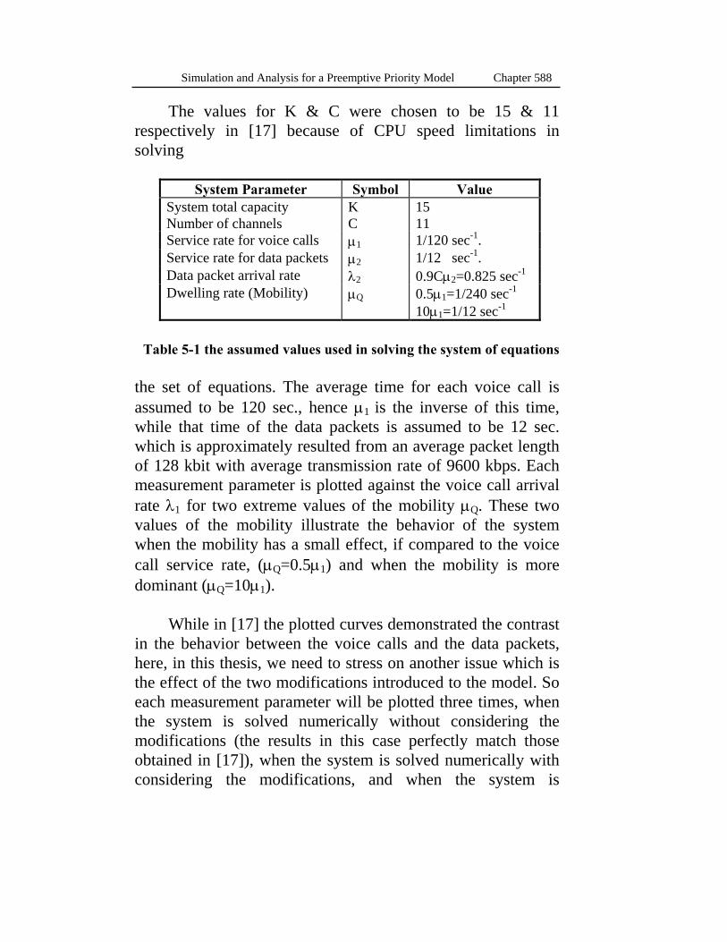
88 Simulation and Analysis for a Preemptive Priority Model Chapter 5
The values for K & C were chosen to be 15 & 11 respectively in [17] because of CPU speed limitations in solving
System Parameter Symbol Value
System total capacity K 15 Number of channels C 11 Service rate for voice calls μ1 1/120 sec-1. Service rate for data packets μ2 1/12 sec-1. Data packet arrival rate λ2 0.9Cμ2=0.825 sec-1 Dwelling rate (Mobility) μQ 0.5μ1=1/240 sec-1
10μ1=1/12 sec-1
Table 5-1 the assumed values used in solving the system of equations the set of equations. The average time for each voice call is assumed to be 120 sec., hence μ1 is the inverse of this time, while that time of the data packets is assumed to be 12 sec. which is approximately resulted from an average packet length of 128 kbit with average transmission rate of 9600 kbps. Each measurement parameter is plotted against the voice call arrival rate λ1 for two extreme values of the mobility μQ. These two values of the mobility illustrate the behavior of the system when the mobility has a small effect, if compared to the voice call service rate, (μQ=0.5μ1) and when the mobility is more dominant (μQ=10μ1).
While in [17] the plotted curves demonstrated the contrast
in the behavior between the voice calls and the data packets, here, in this thesis, we need to stress on another issue which is the effect of the two modifications introduced to the model. So each measurement parameter will be plotted three times, when the system is solved numerically without considering the modifications (the results in this case perfectly match those obtained in [17]), when the system is solved numerically with considering the modifications, and when the system is
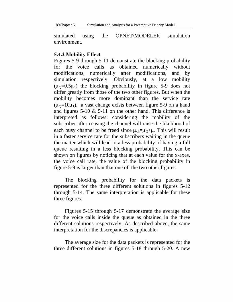
Chapter 5 Simulation and Analysis for a Preemptive Priority Model 89
simulated using the OPNET/MODELER simulation environment.
5.4.2 Mobility Effect Figures 5-9 through 5-11 demonstrate the blocking probability for the voice calls as obtained numerically without modifications, numerically after modifications, and by simulation respectively. Obviously, at a low mobility (μQ=0.5μ1) the blocking probability in figure 5-9 does not differ greatly from those of the two other figures. But when the mobility becomes more dominant than the service rate (μQ=10μ1), a vast change exists between figure 5-9 on a hand and figures 5-10 & 5-11 on the other hand. This difference is interpreted as follows: considering the mobility of the subscriber after ceasing the channel will raise the likelihood of each busy channel to be freed since μch=μQ+μ. This will result in a faster service rate for the subscribers waiting in the queue the matter which will lead to a less probability of having a full queue resulting in a less blocking probability. This can be shown on figures by noticing that at each value for the x-axes, the voice call rate, the value of the blocking probability in figure 5-9 is larger than that one of the two other figures.
The blocking probability for the data packets is
represented for the three different solutions in figures 5-12 through 5-14. The same interpretation is applicable for these three figures.
Figures 5-15 through 5-17 demonstrate the average size for the voice calls inside the queue as obtained in the three different solutions respectively. As described above, the same interpretation for the discrepancies is applicable.
The average size for the data packets is represented for the
three different solutions in figures 5-18 through 5-20. A new
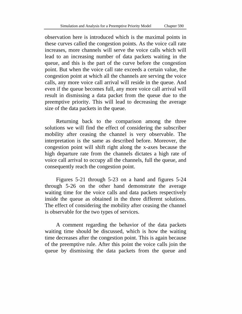
90 Simulation and Analysis for a Preemptive Priority Model Chapter 5
observation here is introduced which is the maximal points in these curves called the congestion points. As the voice call rate increases, more channels will serve the voice calls which will lead to an increasing number of data packets waiting in the queue, and this is the part of the curve before the congestion point. But when the voice call rate exceeds a certain value, the congestion point at which all the channels are serving the voice calls, any more voice call arrival will reside in the queue. And even if the queue becomes full, any more voice call arrival will result in dismissing a data packet from the queue due to the preemptive priority. This will lead to decreasing the average size of the data packets in the queue.
Returning back to the comparison among the three
solutions we will find the effect of considering the subscriber mobility after ceasing the channel is very observable. The interpretation is the same as described before. Moreover, the congestion point will shift right along the x-axes because the high departure rate from the channels dictates a high rate of voice call arrival to occupy all the channels, full the queue, and consequently reach the congestion point.
Figures 5-21 through 5-23 on a hand and figures 5-24
through 5-26 on the other hand demonstrate the average waiting time for the voice calls and data packets respectively inside the queue as obtained in the three different solutions. The effect of considering the mobility after ceasing the channel is observable for the two types of services.
A comment regarding the behavior of the data packets
waiting time should be discussed, which is how the waiting time decreases after the congestion point. This is again because of the preemptive rule. After this point the voice calls join the queue by dismissing the data packets from the queue and

Chapter 5 Simulation and Analysis for a Preemptive Priority Model 91
replace them. Consequently, the data packets no longer wait for a service, the matter which will decrease the waiting time.
Figures 5-27 through 5-29 on a hand and figures 5-30
through 5-32 on the other hand demonstrate the overall blocking probability for the voice calls and data packets respectively as obtained in the three different solutions. As described before, the same comment can be introduced
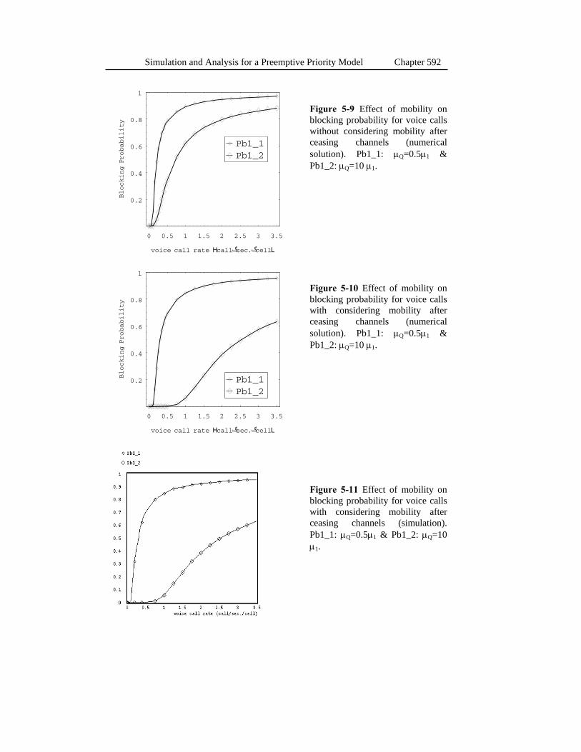
92 Simulation and Analysis for a Preemptive Priority Model Chapter 5
0 0.5 1 1.5 2 2.5 3 3.5
voice call rate Hcallگsec.گcellL
0.2
0.4
0.6
0.8
1
Blocking
Probability
Pb1_2Pb1_1
0 0.5 1 1.5 2 2.5 3 3.5
voice call rate Hcallگsec.گcellL
0.2
0.4
0.6
0.8
1
Blocking
Probability
Pb1_2Pb1_1
Figure 5-9 Effect of mobility on blocking probability for voice calls without considering mobility after ceasing channels (numerical solution). Pb1_1: μQ=0.5μ1 & Pb1_2: μQ=10 μ1. Figure 5-10 Effect of mobility on blocking probability for voice calls with considering mobility after ceasing channels (numerical solution). Pb1_1: μQ=0.5μ1 & Pb1_2: μQ=10 μ1. Figure 5-11 Effect of mobility on blocking probability for voice calls with considering mobility after ceasing channels (simulation). Pb1_1: μQ=0.5μ1 & Pb1_2: μQ=10 μ1.
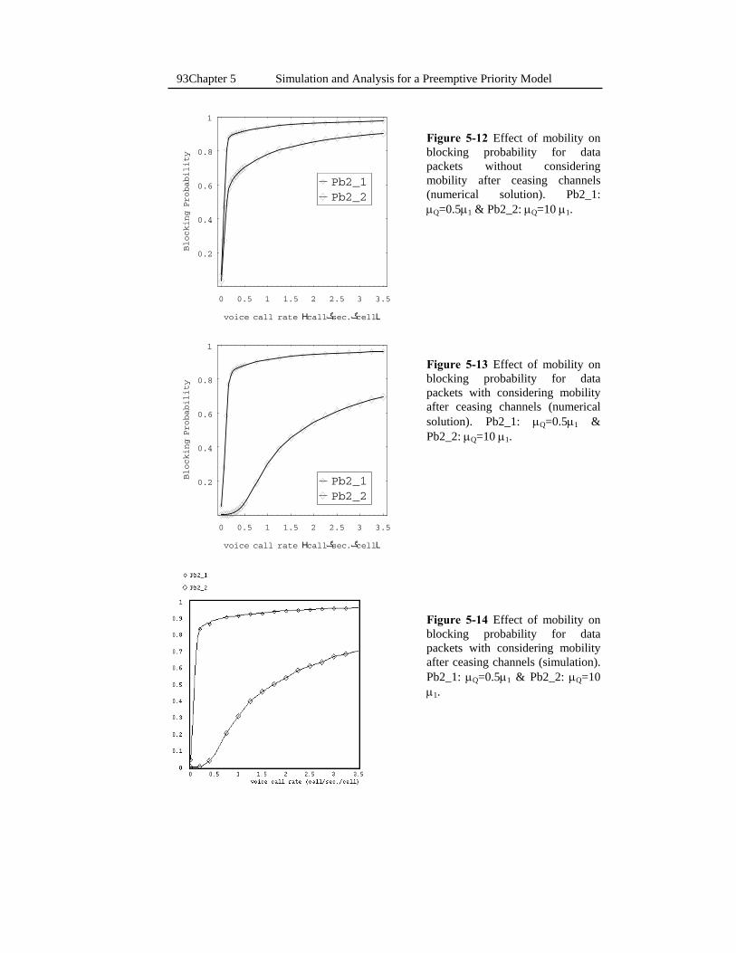
Chapter 5 Simulation and Analysis for a Preemptive Priority Model 93
0 0.5 1 1.5 2 2.5 3 3.5
voice call rate Hcallگsec.گcellL
0.2
0.4
0.6
0.8
1
Blocking
Probability
Pb2_2Pb2_1
0 0.5 1 1.5 2 2.5 3 3.5
voice call rate Hcallگsec.گcellL
0.2
0.4
0.6
0.8
1
Blocking
Probability
Pb2_2Pb2_1
Figure 5-12 Effect of mobility on blocking probability for data packets without considering mobility after ceasing channels (numerical solution). Pb2_1: μQ=0.5μ1 & Pb2_2: μQ=10 μ1. Figure 5-13 Effect of mobility on blocking probability for data packets with considering mobility after ceasing channels (numerical solution). Pb2_1: μQ=0.5μ1 & Pb2_2: μQ=10 μ1. Figure 5-14 Effect of mobility on blocking probability for data packets with considering mobility after ceasing channels (simulation). Pb2_1: μQ=0.5μ1 & Pb2_2: μQ=10 μ1.

94 Simulation and Analysis for a Preemptive Priority Model Chapter 5
0 0.5 1 1.5 2 2.5 3 3.5
voice call rate Hcallگsec.گcellL
0.5
1
1.5
2
2.5
3
3.5
4
Average
Size
in
Queue
EHNq1L_2EHNq1L_1
0 0.5 1 1.5 2 2.5 3 3.5
voice call rate Hcallگsec.گcellL
0.5
1
1.5
2
2.5
3
3.5
4
Average
Size
in
Queue
EHNq1L_2EHNq1L_1
Figure 5-15 Effect of mobility on queue average size for voice calls without considering mobility after ceasing channels (numerical solution). E(Nq1)_1: μQ=0.5μ1 & E(Nq1)_2: μQ=10 μ1. Figure 5-16 Effect of mobility on queue average size for voice calls with considering mobility after ceasing channels (numerical solution). E(Nq1)_1: μQ=0.5μ1 & E(Nq1)_2: μQ=10 μ1. Figure 5-17 Effect of mobility on queue average size for voice calls with considering mobility after ceasing channels (simulation). E(Nq1)_1: μQ=0.5μ1 & E(Nq1)_2: μQ=10 μ1.

Chapter 5 Simulation and Analysis for a Preemptive Priority Model 95
0 0.5 1 1.5 2 2.5 3 3.5
voice call rate Hcallگsec.گcellL
0.5
1
1.5
2
2.5
3
3.5
4
Average
Size
in
Queue
EHNq2L_2EHNq2L_1
0 0.5 1 1.5 2 2.5 3 3.5
voice call rate Hcallگsec.گcellL
0.5
1
1.5
2
2.5
3
3.5
4
Average
Size
in
Queue
EHNq2L_2EHNq2L_1
Figure 5-18 Effect of mobility on queue average size for data packets without considering mobility after ceasing channels (numerical solution). E(Nq2)_1: μQ=0.5μ1 & E(Nq2)_2: μQ=10 μ1. Figure 5-19 Effect of mobility on queue average size for data packets with considering mobility after ceasing channels (numerical solution). E(Nq2)_1: μQ=0.5μ1 & E(Nq2)_2: μQ=10 μ1. Figure 5-20 Effect of mobility on queue average size for data packets with considering mobility after ceasing channels (simulation). E(Nq2)_1: μQ=0.5μ1 & E(Nq2)_2: μQ=10 μ1.
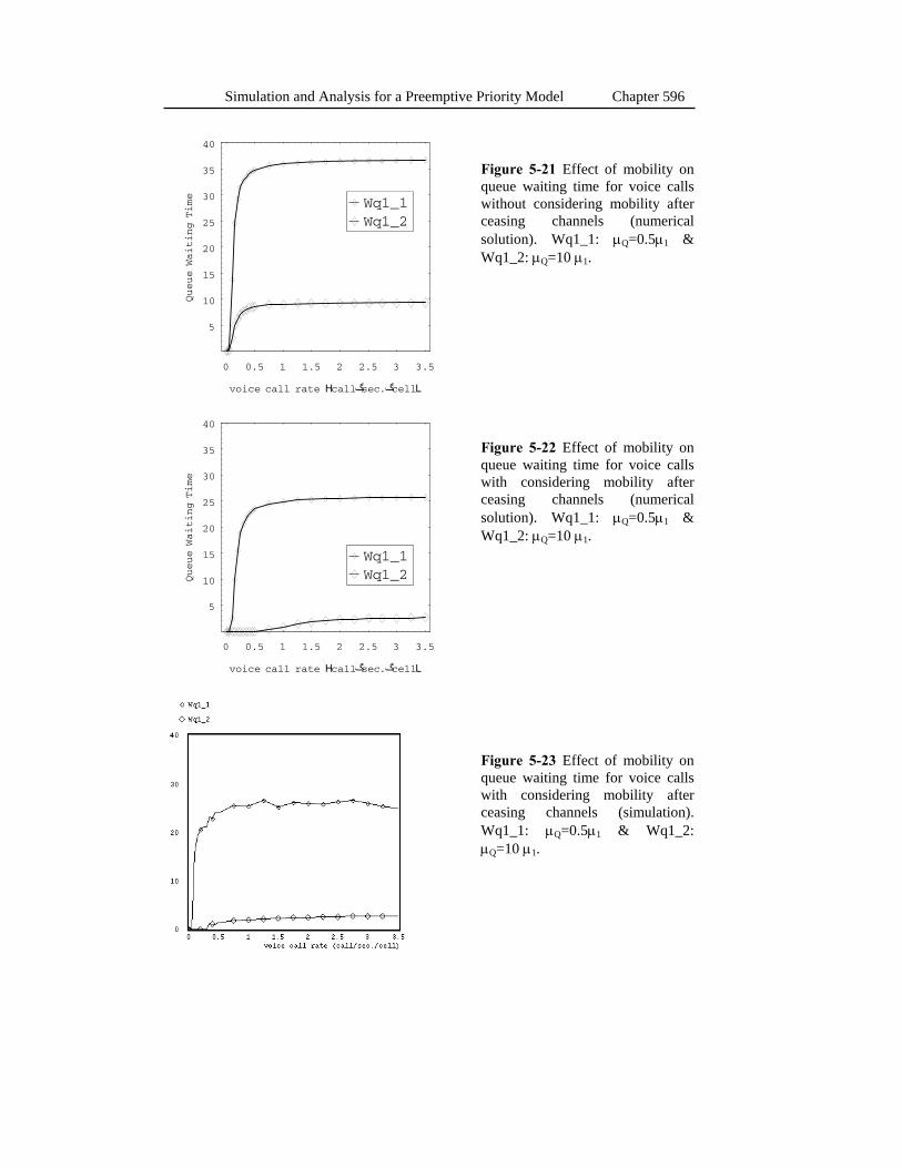
96 Simulation and Analysis for a Preemptive Priority Model Chapter 5
0 0.5 1 1.5 2 2.5 3 3.5
voice call rate Hcallگsec.گcellL
5
10
15
20
25
30
35
40
Queue
Waiting
Time
Wq1_2Wq1_1
0 0.5 1 1.5 2 2.5 3 3.5
voice call rate Hcallگsec.گcellL
5
10
15
20
25
30
35
40
Queue
Waiting
Time
Wq1_2Wq1_1
Figure 5-21 Effect of mobility on queue waiting time for voice calls without considering mobility after ceasing channels (numerical solution). Wq1_1: μQ=0.5μ1 & Wq1_2: μQ=10 μ1. Figure 5-22 Effect of mobility on queue waiting time for voice calls with considering mobility after ceasing channels (numerical solution). Wq1_1: μQ=0.5μ1 & Wq1_2: μQ=10 μ1. Figure 5-23 Effect of mobility on queue waiting time for voice calls with considering mobility after ceasing channels (simulation). Wq1_1: μQ=0.5μ1 & Wq1_2: μQ=10 μ1.
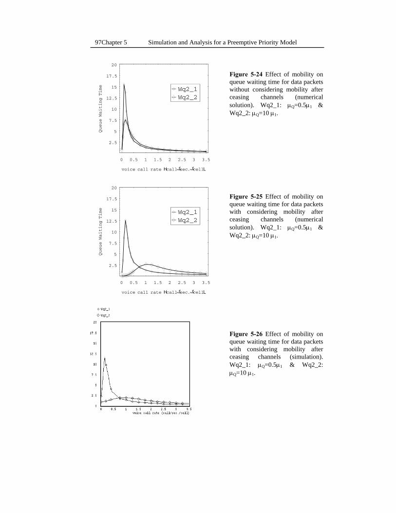
Chapter 5 Simulation and Analysis for a Preemptive Priority Model 97
0 0.5 1 1.5 2 2.5 3 3.5
voice call rate Hcallگsec.گcellL
2.5
5
7.5
10
12.5
15
17.5
20
Queue
Waiting
Time
Wq2_2Wq2_1
0 0.5 1 1.5 2 2.5 3 3.5
voice call rate Hcallگsec.گcellL
2.5
5
7.5
10
12.5
15
17.5
20
Queue
Waiting
Time
Wq2_2Wq2_1
Figure 5-24 Effect of mobility on queue waiting time for data packets without considering mobility after ceasing channels (numerical solution). Wq2_1: μQ=0.5μ1 & Wq2_2: μQ=10 μ1. Figure 5-25 Effect of mobility on queue waiting time for data packets with considering mobility after ceasing channels (numerical solution). Wq2_1: μQ=0.5μ1 & Wq2_2: μQ=10 μ1. Figure 5-26 Effect of mobility on queue waiting time for data packets with considering mobility after ceasing channels (simulation). Wq2_1: μQ=0.5μ1 & Wq2_2: μQ=10 μ1.
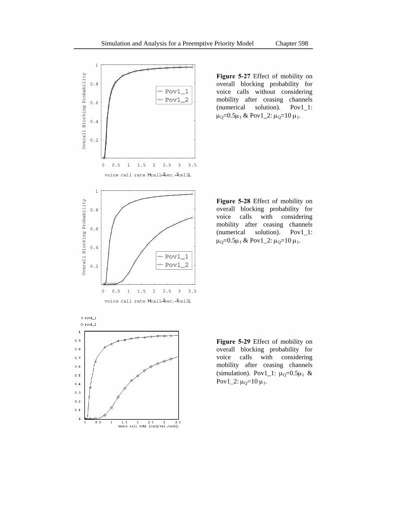
98 Simulation and Analysis for a Preemptive Priority Model Chapter 5
0 0.5 1 1.5 2 2.5 3 3.5
voice call rate Hcallگsec.گcellL
0.2
0.4
0.6
0.8
1
Overall
Blocking
Probability
Pov1_2Pov1_1
0 0.5 1 1.5 2 2.5 3 3.5
voice call rate Hcallگsec.گcellL
0.2
0.4
0.6
0.8
1
Overall
Blocking
Probability
Pov1_2Pov1_1
Figure 5-27 Effect of mobility on overall blocking probability for voice calls without considering mobility after ceasing channels (numerical solution). Pov1_1: μQ=0.5μ1 & Pov1_2: μQ=10 μ1. Figure 5-28 Effect of mobility on overall blocking probability for voice calls with considering mobility after ceasing channels (numerical solution). Pov1_1: μQ=0.5μ1 & Pov1_2: μQ=10 μ1. Figure 5-29 Effect of mobility on overall blocking probability for voice calls with considering mobility after ceasing channels (simulation). Pov1_1: μQ=0.5μ1 & Pov1_2: μQ=10 μ1.
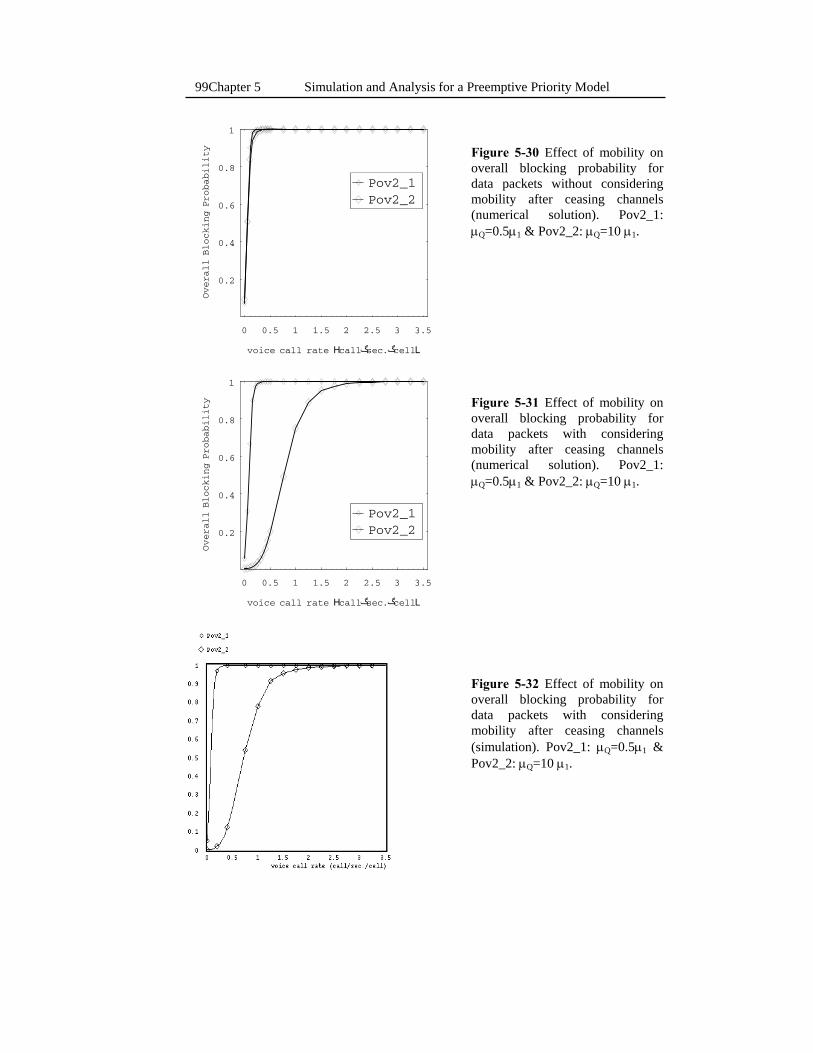
Chapter 5 Simulation and Analysis for a Preemptive Priority Model 99
0 0.5 1 1.5 2 2.5 3 3.5
voice call rate Hcallگsec.گcellL
0.2
0.4
0.6
0.8
1
Overall
Blocking
Probability
Pov2_2Pov2_1
0 0.5 1 1.5 2 2.5 3 3.5
voice call rate Hcallگsec.گcellL
0.2
0.4
0.6
0.8
1
Overall
Blocking
Probability
Pov2_2Pov2_1
Figure 5-30 Effect of mobility on overall blocking probability for data packets without considering mobility after ceasing channels (numerical solution). Pov2_1: μQ=0.5μ1 & Pov2_2: μQ=10 μ1. Figure 5-31 Effect of mobility on overall blocking probability for data packets with considering mobility after ceasing channels (numerical solution). Pov2_1: μQ=0.5μ1 & Pov2_2: μQ=10 μ1. Figure 5-32 Effect of mobility on overall blocking probability for data packets with considering mobility after ceasing channels (simulation). Pov2_1: μQ=0.5μ1 & Pov2_2: μQ=10 μ1.
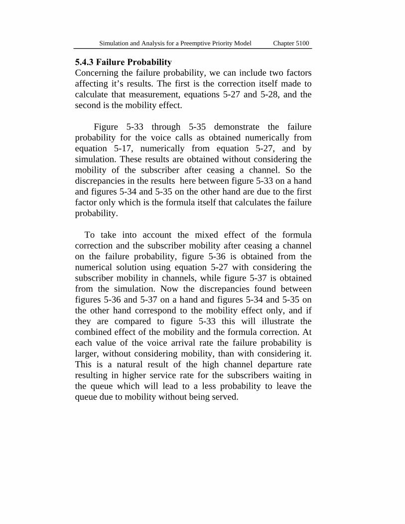
100 Simulation and Analysis for a Preemptive Priority Model Chapter 5
5.4.3 Failure Probability Concerning the failure probability, we can include two factors affecting it’s results. The first is the correction itself made to calculate that measurement, equations 5-27 and 5-28, and the second is the mobility effect.
Figure 5-33 through 5-35 demonstrate the failure probability for the voice calls as obtained numerically from equation 5-17, numerically from equation 5-27, and by simulation. These results are obtained without considering the mobility of the subscriber after ceasing a channel. So the discrepancies in the results here between figure 5-33 on a hand and figures 5-34 and 5-35 on the other hand are due to the first factor only which is the formula itself that calculates the failure probability.
To take into account the mixed effect of the formula
correction and the subscriber mobility after ceasing a channel on the failure probability, figure 5-36 is obtained from the numerical solution using equation 5-27 with considering the subscriber mobility in channels, while figure 5-37 is obtained from the simulation. Now the discrepancies found between figures 5-36 and 5-37 on a hand and figures 5-34 and 5-35 on the other hand correspond to the mobility effect only, and if they are compared to figure 5-33 this will illustrate the combined effect of the mobility and the formula correction. At each value of the voice arrival rate the failure probability is larger, without considering mobility, than with considering it. This is a natural result of the high channel departure rate resulting in higher service rate for the subscribers waiting in the queue which will lead to a less probability to leave the queue due to mobility without being served.
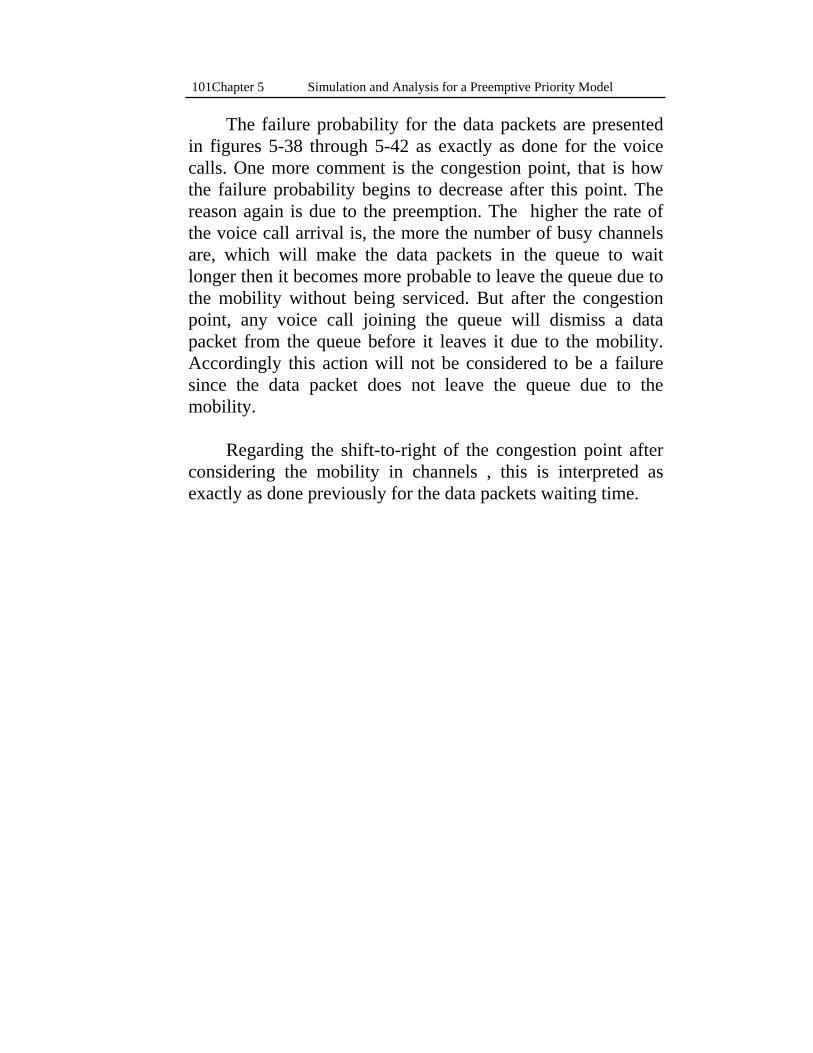
Chapter 5 Simulation and Analysis for a Preemptive Priority Model 101
The failure probability for the data packets are presented in figures 5-38 through 5-42 as exactly as done for the voice calls. One more comment is the congestion point, that is how the failure probability begins to decrease after this point. The reason again is due to the preemption. The higher the rate of the voice call arrival is, the more the number of busy channels are, which will make the data packets in the queue to wait longer then it becomes more probable to leave the queue due to the mobility without being serviced. But after the congestion point, any voice call joining the queue will dismiss a data packet from the queue before it leaves it due to the mobility. Accordingly this action will not be considered to be a failure since the data packet does not leave the queue due to the mobility.
Regarding the shift-to-right of the congestion point after
considering the mobility in channels , this is interpreted as exactly as done previously for the data packets waiting time.

102 Simulation and Analysis for a Preemptive Priority Model Chapter 5
0 0.5 1 1.5 2 2.5 3 3.5
voice call rate Hcallگsec.گcellL
0.1
0.2
0.3
0.4
0.5
0.6
0.7
0.8
Failure
Probability
Pf1_2Pf1_1
0 0.5 1 1.5 2 2.5 3 3.5
voice call rate Hcallگsec.گcellL
0.1
0.2
0.3
0.4
0.5
0.6
0.7
0.8
Failure
Probability
Pf1_2Pf1_1
Figure 5-33 Effect of mobility on failure probability (equation 5-17) for voice calls without considering mobility after ceasing channels (numerical solution). Pf2_1: μQ=0.5μ1 & Pf2_2: μQ=10 μ1. Figure 5-34 Effect of mobility on failure probability (equation 5-27) for voice calls without considering mobility after ceasing channels (numerical solution). Pf2_1: μQ=0.5μ1 & Pf2_2: μQ=10 μ1. Figure 5-35 Effect of mobility on failure probability for voice calls without considering mobility in channels (simulation). Pf2_1: μQ=0.5μ1 & Pf2_2: μQ=10 μ1
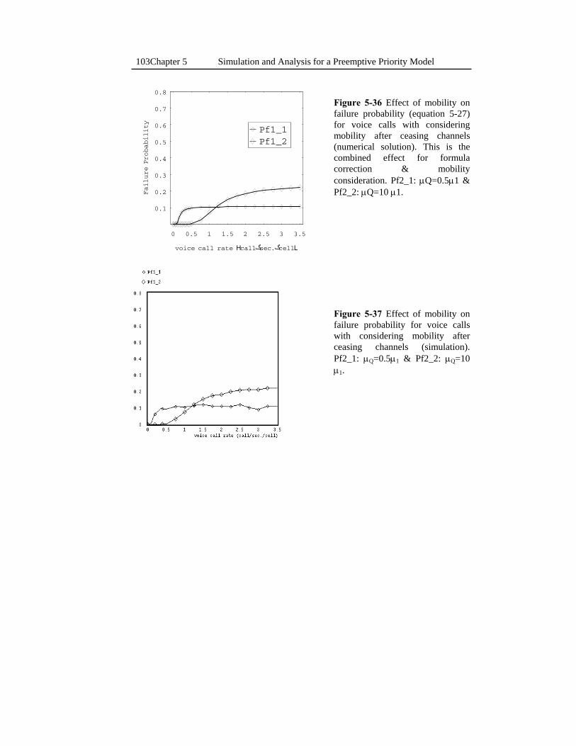
Chapter 5 Simulation and Analysis for a Preemptive Priority Model 103
0 0.5 1 1.5 2 2.5 3 3.5
voice call rate Hcallگsec.گcellL
0.1
0.2
0.3
0.4
0.5
0.6
0.7
0.8
Failure
Probability
Pf1_2Pf1_1
Figure 5-36 Effect of mobility on failure probability (equation 5-27) for voice calls with considering mobility after ceasing channels (numerical solution). This is the combined effect for formula correction & mobility consideration. Pf2_1: μQ=0.5μ1 & Pf2_2: μQ=10 μ1.
Figure 5-37 Effect of mobility on failure probability for voice calls with considering mobility after ceasing channels (simulation). Pf2_1: μQ=0.5μ1 & Pf2_2: μQ=10 μ1.

104 Simulation and Analysis for a Preemptive Priority Model Chapter 5
0 0.5 1 1.5 2 2.5 3 3.5
voice call rate Hcallگsec.گcellL
0.1
0.2
0.3
0.4
0.5
0.6
Failure
Probability
Pf2_2Pf2_1
0 0.5 1 1.5 2 2.5 3 3.5
voice call rate Hcallگsec.گcellL
0.1
0.2
0.3
0.4
0.5
0.6
Failure
Probability
Pf2_2Pf2_1
Figure 5-38 Effect of mobility on failure probability (equation 5-18) for data packets without considering mobility after ceasing channels (numerical solution). Pf2_1: μQ=0.5μ1 & Pf2_2: μQ=10 μ1. Figure 5-39 Effect of mobility on failure probability (equation 5-28) for data packets without considering mobility after ceasing channels (numerical solution) Pf2_1: μQ=0.5μ1 & Pf2_2: μQ=10 μ1. Figure 5-40 Effect of mobility on failure probability for data packets without considering mobility in channels (simulation). Pf2_1: μQ=0.5μ1 & Pf2_2: μQ=10 μ1

Chapter 5 Simulation and Analysis for a Preemptive Priority Model 105
0 0.5 1 1.5 2 2.5 3 3.5
voice call rate Hcallگsec.گcellL
0.1
0.2
0.3
0.4
0.5
0.6
Failure
Probability
Pf2_2Pf2_1
Figure 5-41 Effect of mobility on failure probability (equation 5-28) for data packets with considering mobility after ceasing channels (numerical solution). This is the combined effect for formula correction & mobility consideration. Pf2_1: μQ=0.5μ1 & Pf2_2: μQ=10 μ1.
Figure 5-42 Effect of mobility on failure probability for data packets considering mobility after ceasing channels (simulation). Pf2_1: μQ=0.5μ1 & Pf2_2: μQ=10 μ1.
Chapter 6
Conclusion and Future Work
preemptive priority model proposed in the literature is studied in this thesis. Two mathematical modifications are introduced to the model, then the model is solved
mathematically. Also, simulation is carried out to validate the mathematical solution. A complete matching between the results of the simulation and the mathematical solution (after modifications) is observed, while these results on a hand indicate considerable discrepancies from those results obtained after solving the model without considering these modifications.
One of the mathematical modifications concerns the equation that calculates the probability of the users to fail ceasing the channel due to their mobility after joining the queue. The second modification is considering the mobility effect of the users after ceasing the channel and being served.
From what briefly stated above we conclude the
following: • The mobility of the user is an important parameter
affecting the performance of the cellular mobile radio networks when prioritization is applied.
• Both, simulation besides mathematical solution, can validate the work and put it at a high degree of confidence.
• As a general, flexible, and very powerful tool in discrete-event simulation, OPNET is very suggested to any researcher or system analyzer who analyzes or designs any discrete-even system generally, or networks, specially.
A
Chapter 6 Conclusion and Future Work 107
Because science has an evolutionary nature, one should not start where others began. Instead, one should start from the last step made. The future work concerning the prioritization in the cellular mobile radio networks could be one of the following:
• Taking into account the case of a multi-cell system. That is to consider the system as a complete CGSA (not necessary to be a real-life implementation for a typical geographical area) to study the effect of neighboring cells.
• Carrying out the simulation for the above point. If the OPNET simulation environment is used as the simulation tool, this will make the model of simulation to be a multi-node model since each cell will be represented as a single node.
• The values assumed here, in this thesis, are not expressing a practical system because of two reasons. The first is to compare our results with the results obtained in [17]. The second is the difficulties of accessing the practical values. It is very probable to have different results for the measurement parameters if the practical values of the system parameters are used instead. One possible future work is to consider the parameters for practical systems and propose modifications in the prioritization models accordingly if necessary.
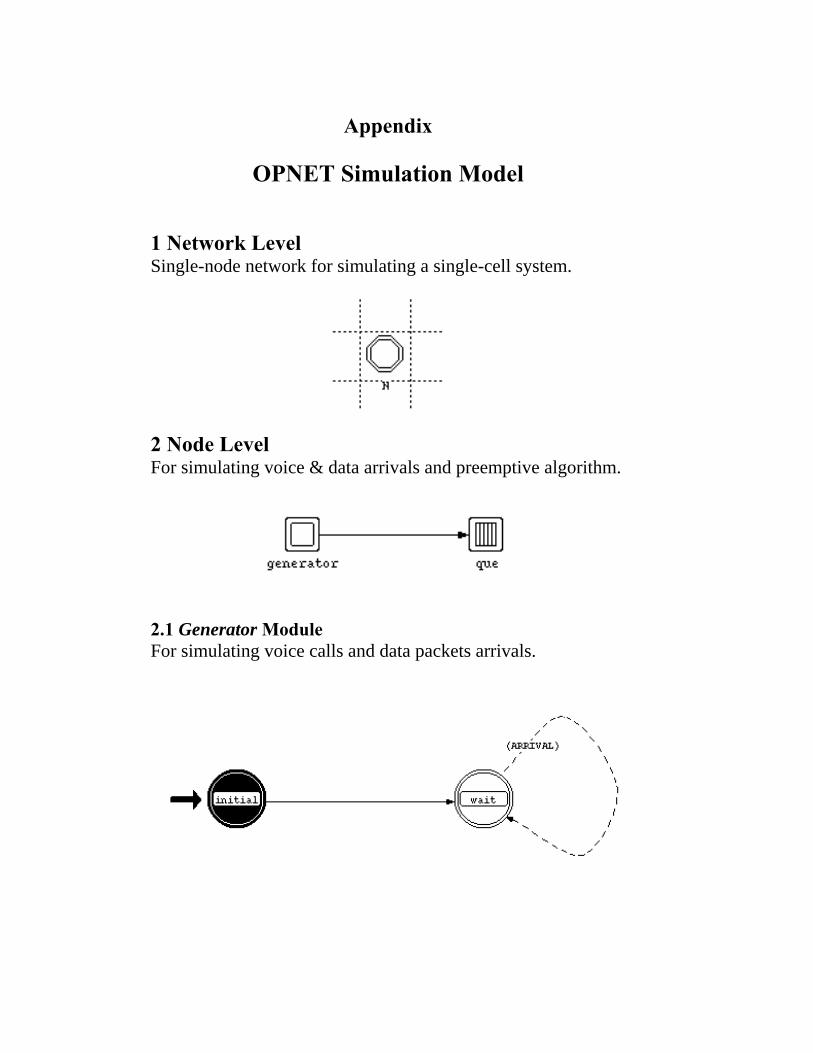
Appendix
OPNET Simulation Model 1 Network Level Single-node network for simulating a single-cell system.
2 Node Level For simulating voice & data arrivals and preemptive algorithm.
2.1 Generator Module For simulating voice calls and data packets arrivals.
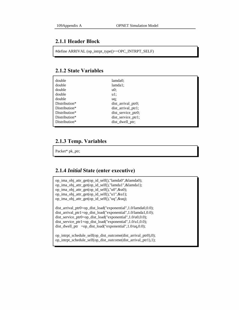
Appendix A OPNET Simulation Model 109
2.1.1 Header Block #define ARRIVAL (op_intrpt_type()==OPC_INTRPT_SELF) 2.1.2 State Variables double lamda0; double lamda1; double u0; double u1; double uq; Distribution* dist_arrival_ptr0; Distribution* dist_arrival_ptr1; Distribution* dist_service_ptr0; Distribution* dist_service_ptr1; Distribution* dist_dwell_ptr; 2.1.3 Temp. Variables Packet* pk_ptr; 2.1.4 Initial State (enter executive) op_ima_obj_attr_get(op_id_self(),"lamda0",&lamda0); op_ima_obj_attr_get(op_id_self(),"lamda1",&lamda1); op_ima_obj_attr_get(op_id_self(),"u0",&u0); op_ima_obj_attr_get(op_id_self(),"u1",&u1); op_ima_obj_attr_get(op_id_self(),"uq",&uq); dist_arrival_ptr0=op_dist_load("exponential",1.0/lamda0,0.0); dist_arrival_ptr1=op_dist_load("exponential",1.0/lamda1,0.0); dist_service_ptr0=op_dist_load("exponential",1.0/u0,0.0); dist_service_ptr1=op_dist_load("exponential",1.0/u1,0.0); dist_dwell_ptr =op_dist_load("exponential",1.0/uq,0.0); op_intrpt_schedule_self(op_dist_outcome(dist_arrival_ptr0),0); op_intrpt_schedule_self(op_dist_outcome(dist_arrival_ptr1),1);

110 OPNET Simulation Model Appendix A
2.1.5 Wait State (enter executive) pk_ptr=op_pk_create(1); if (op_intrpt_code()==0){
op_pk_priority_set(pk_ptr,0); op_pk_fd_set(pk_ptr,0,OPC_FIELD_TYPE_DOUBLE,
op_dist_outcome(dist_service_ptr0),0); op_pk_fd_set(pk_ptr,1,OPC_FIELD_TYPE_DOUBLE, op_dist_outcome(dist_dwell_ptr),0); op_pk_send(pk_ptr,0); op_intrpt_schedule_self(op_sim_time()+op_dist_outcome(dist_arrival_ptr0),0); } else{
op_pk_priority_set(pk_ptr,1); op_pk_fd_set(pk_ptr,0,OPC_FIELD_TYPE_DOUBLE,op_dist_outcome
(dist_service_ptr1),0); op_pk_fd_set(pk_ptr,1,OPC_FIELD_TYPE_DOUBLE,op_dist_outcome
(dist_dwell_ptr),0); op_pk_send(pk_ptr,0); op_intrpt_schedule_self(op_sim_time()+op_dist_outcome(dist_arrival_ptr1),1); } 2.2 Que Module For simulating the preemptive algorithm.
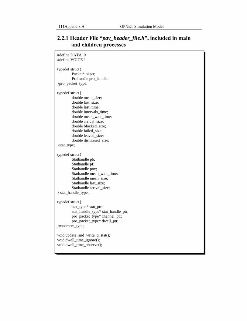
Appendix A OPNET Simulation Model 111
2.2.1 Header File “pav_header_file.h”, included in main and children processes #define DATA 0 #define VOICE 1 typedef struct{ Packet* pkptr; Prohandle pro_handle; }pro_packet_type; typedef struct{ double mean_size;
double last_size; double last_time; double intervals_time; double mean_wait_time; double arrival_size; double blocked_size; double failed_size; double leaved_size;
double dismissed_size; }stat_type; typedef struct{ Stathandle pb; Stathandle pf; Stathandle pov; Stathandle mean_wait_time; Stathandle mean_size; Stathandle last_size; Stathandle arrival_size; } stat_handle_type; typedef struct{ stat_type* stat_ptr; stat_handle_type* stat_handle_ptr; pro_packet_type* channel_ptr; pro_packet_type* dwell_ptr; }modmem_type; void update_and_write_q_stat(); void dwell_time_ignore(); void dwell_time_observe();

112 OPNET Simulation Model Appendix A
2.2.2 Header Block #include"pav_header_file.h" #define CALL_ARRIVAL (op_intrpt_type()==OPC_INTRPT_STRM) #define CHANNEL_FREE (op_intrpt_type()==OPC_INTRPT_PROCESS) #define END_SIMULATION (op_intrpt_type()==OPC_INTRPT_ENDSIM) 2.2.3 State Variables int K; int C; int call_types; int current_priority; int i; Packet* current_ptr; Packet* temp_pkptr; pro_packet_type* channel_arr; pro_packet_type* dwell_arr; stat_type* stat_arr; stat_handle_type* stat_handle_arr; 2.2.4 Temp. Variables modmem_type* modmem_ptr; 2.2.5 Function Block void update_and_write_q_stat(stat_handle_type* handle_arr,stat_type* arr,
Packet* ptr,int insertion){ double enterance_time;
int priority;
priority=op_pk_priority_get(ptr); arr[priority].mean_size+=arr[priority].last_size*(op_sim_time()- arr[priority].last_time);
arr[priority].intervals_time+=op_sim_time()-arr[priority].last_time; arr[priority].last_time=op_sim_time(); if (insertion){ arr[priority].last_size++; op_pk_fd_set(ptr,2,OPC_FIELD_TYPE_DOUBLE,op_sim_time(),0); }
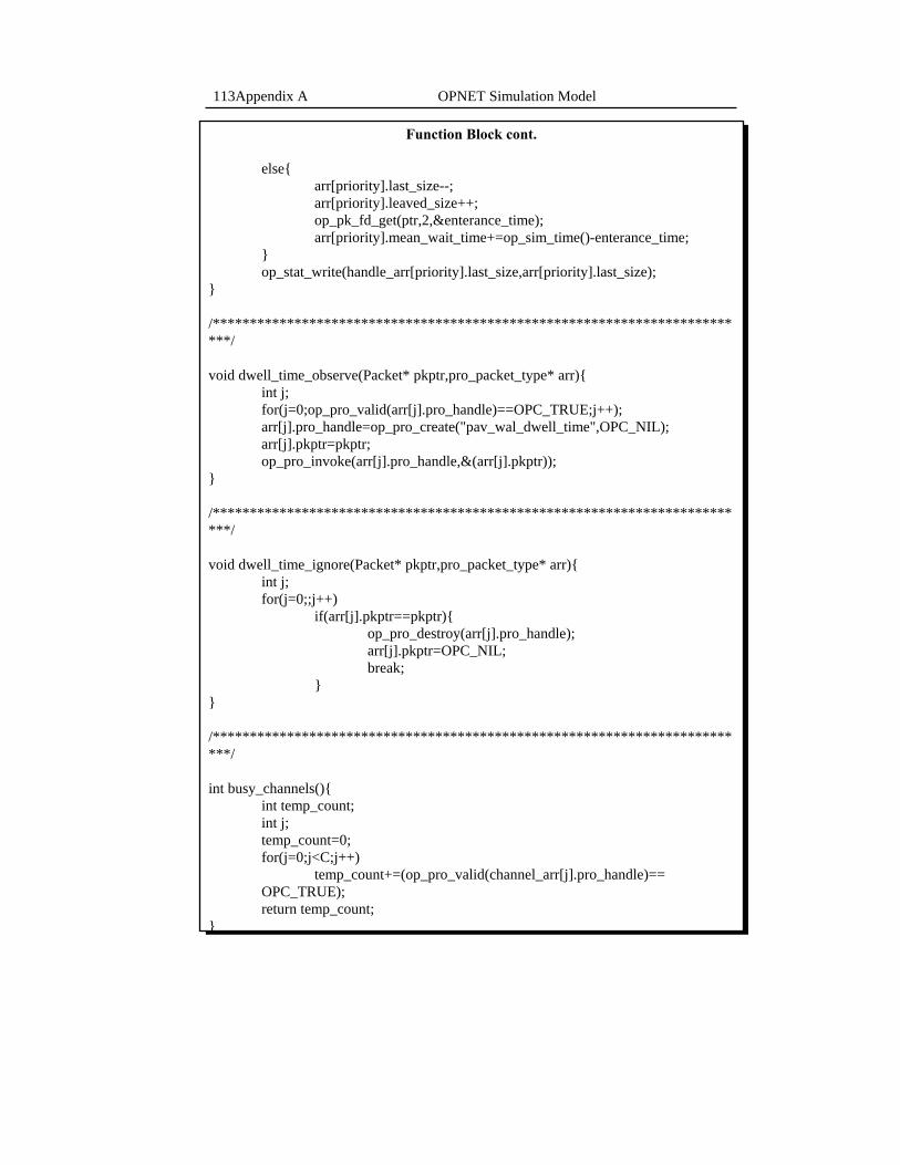
Appendix A OPNET Simulation Model 113
Function Block cont.
else{ arr[priority].last_size--; arr[priority].leaved_size++; op_pk_fd_get(ptr,2,&enterance_time); arr[priority].mean_wait_time+=op_sim_time()-enterance_time; } op_stat_write(handle_arr[priority].last_size,arr[priority].last_size); } /*************************************************************************/ void dwell_time_observe(Packet* pkptr,pro_packet_type* arr){ int j; for(j=0;op_pro_valid(arr[j].pro_handle)==OPC_TRUE;j++); arr[j].pro_handle=op_pro_create("pav_wal_dwell_time",OPC_NIL); arr[j].pkptr=pkptr; op_pro_invoke(arr[j].pro_handle,&(arr[j].pkptr)); } /*************************************************************************/ void dwell_time_ignore(Packet* pkptr,pro_packet_type* arr){ int j; for(j=0;;j++) if(arr[j].pkptr==pkptr){ op_pro_destroy(arr[j].pro_handle); arr[j].pkptr=OPC_NIL; break; } } /*************************************************************************/ int busy_channels(){ int temp_count; int j; temp_count=0; for(j=0;j<C;j++)
temp_count+=(op_pro_valid(channel_arr[j].pro_handle)== OPC_TRUE);
return temp_count; }
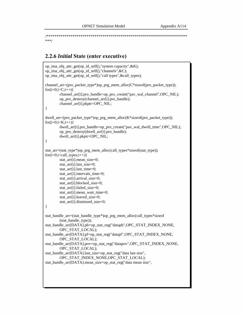
114 OPNET Simulation Model Appendix A
/*************************************************************************/ 2.2.6 Initial State (enter executive) op_ima_obj_attr_get(op_id_self(),"system capacity",&K); op_ima_obj_attr_get(op_id_self(),"channels",&C); op_ima_obj_attr_get(op_id_self(),"call types",&call_types); channel_arr=(pro_packet_type*)op_prg_mem_alloc(C*sizeof(pro_packet_type)); for(i=0;i<C;i++){
channel_arr[i].pro_handle=op_pro_create("pav_wal_channel",OPC_NIL); op_pro_destroy(channel_arr[i].pro_handle); channel_arr[i].pkptr=OPC_NIL; } dwell_arr=(pro_packet_type*)op_prg_mem_alloc(K*sizeof(pro_packet_type)); for(i=0;i<K;i++){
dwell_arr[i].pro_handle=op_pro_create("pav_wal_dwell_time",OPC_NIL); op_pro_destroy(dwell_arr[i].pro_handle); dwell_arr[i].pkptr=OPC_NIL; } stat_arr=(stat_type*)op_prg_mem_alloc(call_types*sizeof(stat_type)); for(i=0;i<call_types;i++){ stat_arr[i].mean_size=0; stat_arr[i].last_size=0; stat_arr[i].last_time=0; stat_arr[i].intervals_time=0; stat_arr[i].arrival_size=0; stat_arr[i].blocked_size=0; stat_arr[i].failed_size=0; stat_arr[i].mean_wait_time=0; stat_arr[i].leaved_size=0; stat_arr[i].dismissed_size=0; } stat_handle_arr=(stat_handle_type*)op_prg_mem_alloc(call_types*sizeof
(stat_handle_type)); stat_handle_arr[DATA].pb=op_stat_reg("datapb",OPC_STAT_INDEX_NONE,
OPC_STAT_LOCAL); stat_handle_arr[DATA].pf=op_stat_reg("datapf",OPC_STAT_INDEX_NONE,
OPC_STAT_LOCAL); stat_handle_arr[DATA].pov=op_stat_reg("datapov",OPC_STAT_INDEX_NONE,
OPC_STAT_LOCAL); stat_handle_arr[DATA].last_size=op_stat_reg("data last size",
OPC_STAT_INDEX_NONE,OPC_STAT_LOCAL); stat_handle_arr[DATA].mean_size=op_stat_reg("data mean size",
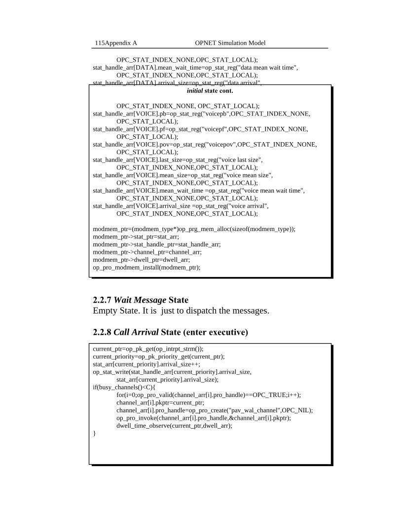
Appendix A OPNET Simulation Model 115
OPC_STAT_INDEX_NONE,OPC_STAT_LOCAL); stat_handle_arr[DATA].mean_wait_time=op_stat_reg("data mean wait time",
OPC_STAT_INDEX_NONE,OPC_STAT_LOCAL); stat_handle_arr[DATA].arrival_size=op_stat_reg("data arrival",
initial state cont.
OPC_STAT_INDEX_NONE, OPC_STAT_LOCAL); stat_handle_arr[VOICE].pb=op_stat_reg("voicepb",OPC_STAT_INDEX_NONE,
OPC_STAT_LOCAL); stat_handle_arr[VOICE].pf=op_stat_reg("voicepf",OPC_STAT_INDEX_NONE,
OPC_STAT_LOCAL); stat_handle_arr[VOICE].pov=op_stat_reg("voicepov",OPC_STAT_INDEX_NONE,
OPC_STAT_LOCAL); stat_handle_arr[VOICE].last_size=op_stat_reg("voice last size",
OPC_STAT_INDEX_NONE,OPC_STAT_LOCAL); stat_handle_arr[VOICE].mean_size=op_stat_reg("voice mean size",
OPC_STAT_INDEX_NONE,OPC_STAT_LOCAL); stat_handle_arr[VOICE].mean_wait_time =op_stat_reg("voice mean wait time",
OPC_STAT_INDEX_NONE,OPC_STAT_LOCAL); stat_handle_arr[VOICE].arrival_size =op_stat_reg("voice arrival",
OPC_STAT_INDEX_NONE,OPC_STAT_LOCAL); modmem_ptr=(modmem_type*)op_prg_mem_alloc(sizeof(modmem_type)); modmem_ptr->stat_ptr=stat_arr; modmem_ptr->stat_handle_ptr=stat_handle_arr; modmem_ptr->channel_ptr=channel_arr; modmem_ptr->dwell_ptr=dwell_arr; op_pro_modmem_install(modmem_ptr); 2.2.7 Wait Message State Empty State. It is just to dispatch the messages. 2.2.8 Call Arrival State (enter executive) current_ptr=op_pk_get(op_intrpt_strm()); current_priority=op_pk_priority_get(current_ptr); stat_arr[current_priority].arrival_size++; op_stat_write(stat_handle_arr[current_priority].arrival_size,
stat_arr[current_priority].arrival_size); if(busy_channels()<C){ for(i=0;op_pro_valid(channel_arr[i].pro_handle)==OPC_TRUE;i++); channel_arr[i].pkptr=current_ptr; channel_arr[i].pro_handle=op_pro_create("pav_wal_channel",OPC_NIL); op_pro_invoke(channel_arr[i].pro_handle,&channel_arr[i].pkptr); dwell_time_observe(current_ptr,dwell_arr); }

116 OPNET Simulation Model Appendix A
else{ /********************CHANNEL IS BUSY********************* */
for(i=0;i<C;i++) if(op_pk_priority_get(channel_arr[i].pkptr)==DATA) break;
call arrival state cont.
if(op_subq_stat(0,OPC_QSTAT_PKSIZE)<K-C) /*QUEUE IS NOT FULL*/ if(current_priority==VOICE && i<C){
op_pro_destroy(channel_arr[i].pro_handle); op_subq_pk_insert(0,channel_arr[i].pkptr, OPC_QPOS_PRIO); update_and_write_q_stat(stat_handle_arr,stat_arr, channel_arr[i].pkptr,1);
channel_arr[i].pkptr=current_ptr; channel_arr[i].pro_handle=op_pro_create ("pav_wal_channel",OPC_NIL);
dwell_time_observe(current_ptr,dwell_arr); op_pro_invoke(channel_arr[i].pro_handle, &channel_arr[i].pkptr);
} else{
op_subq_pk_insert(0,current_ptr, OPC_QPOS_PRIO);
dwell_time_observe(current_ptr,dwell_arr); update_and_write_q_stat(stat_handle_arr,stat_arr, current_ptr,1);
} else /*******QUEUE IS FULL******** */ if(current_priority==VOICE && i<C){ dwell_time_ignore(channel_arr[i].pkptr,dwell_arr); op_pro_destroy(channel_arr[i].pro_handle); op_pk_destroy(channel_arr[i].pkptr); stat_arr[DATA].dismissed_size++; channel_arr[i].pkptr=current_ptr;
channel_arr[i].pro_handle=op_pro_create ("pav_wal_channel",OPC_NIL); op_pro_invoke(channel_arr[i].pro_handle, &channel_arr[i].pkptr);
dwell_time_observe(current_ptr,dwell_arr); } else{
temp_pkptr=op_subq_pk_access(0, OPC_QPOS_TAIL);
if(current_priority==VOICE && op_pk_priority_get(temp_pkptr)==DATA)
{ op_subq_pk_remove(0,OPC_QPOS_TAIL;
dwell_time_ignore(temp_pkptr,dwell_arr); update_and_write_q_stat(stat_handle_arr,
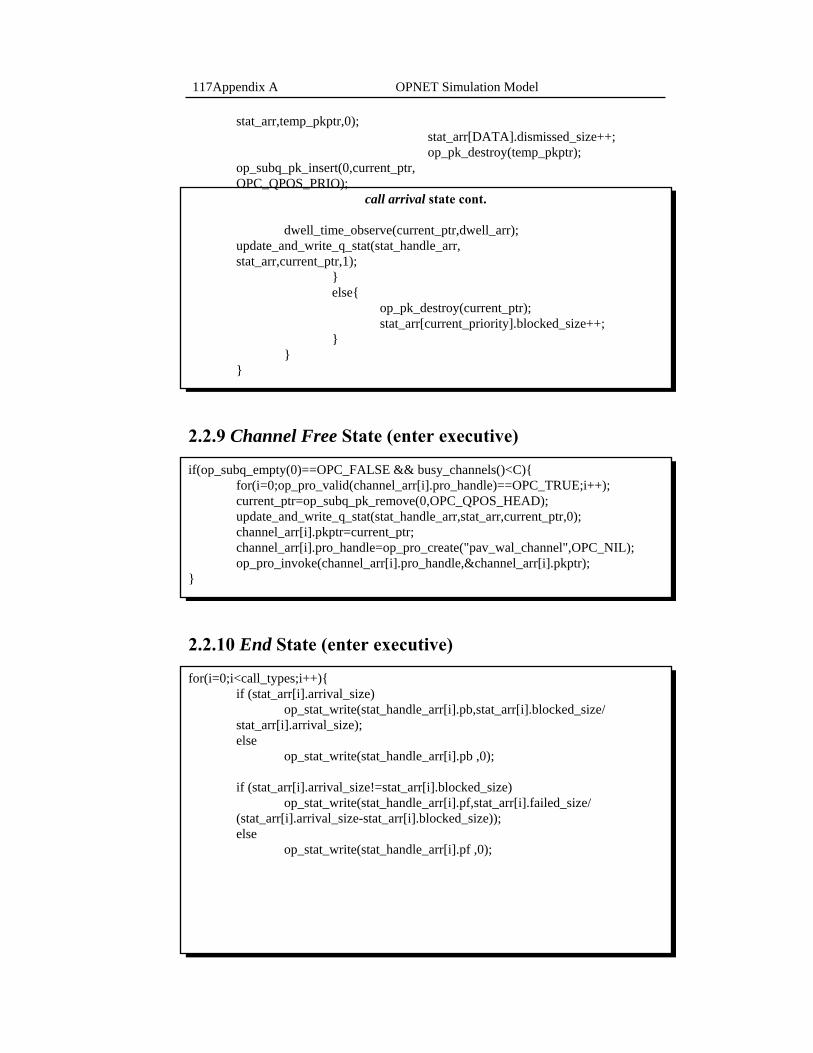
Appendix A OPNET Simulation Model 117
stat_arr,temp_pkptr,0); stat_arr[DATA].dismissed_size++; op_pk_destroy(temp_pkptr);
op_subq_pk_insert(0,current_ptr, OPC_QPOS_PRIO);
call arrival state cont. dwell_time_observe(current_ptr,dwell_arr); update_and_write_q_stat(stat_handle_arr, stat_arr,current_ptr,1);
} else{ op_pk_destroy(current_ptr); stat_arr[current_priority].blocked_size++; } } } 2.2.9 Channel Free State (enter executive) if(op_subq_empty(0)==OPC_FALSE && busy_channels()<C){
for(i=0;op_pro_valid(channel_arr[i].pro_handle)==OPC_TRUE;i++); current_ptr=op_subq_pk_remove(0,OPC_QPOS_HEAD); update_and_write_q_stat(stat_handle_arr,stat_arr,current_ptr,0); channel_arr[i].pkptr=current_ptr; channel_arr[i].pro_handle=op_pro_create("pav_wal_channel",OPC_NIL); op_pro_invoke(channel_arr[i].pro_handle,&channel_arr[i].pkptr); } 2.2.10 End State (enter executive) for(i=0;i<call_types;i++){
if (stat_arr[i].arrival_size) op_stat_write(stat_handle_arr[i].pb,stat_arr[i].blocked_size/ stat_arr[i].arrival_size);
else op_stat_write(stat_handle_arr[i].pb ,0); if (stat_arr[i].arrival_size!=stat_arr[i].blocked_size)
op_stat_write(stat_handle_arr[i].pf,stat_arr[i].failed_size/ (stat_arr[i].arrival_size-stat_arr[i].blocked_size));
else op_stat_write(stat_handle_arr[i].pf ,0);
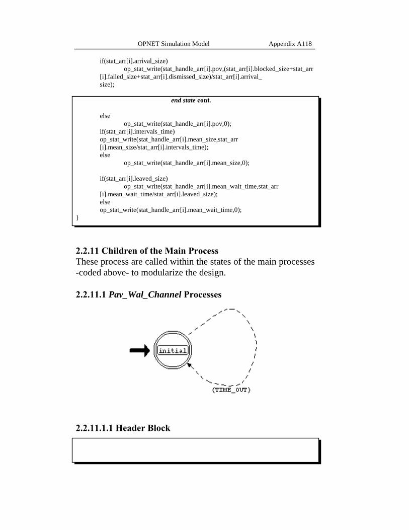
118 OPNET Simulation Model Appendix A
if(stat_arr[i].arrival_size) op_stat_write(stat_handle_arr[i].pov,(stat_arr[i].blocked_size+stat_arr [i].failed_size+stat_arr[i].dismissed_size)/stat_arr[i].arrival_ size);
end state cont.
else op_stat_write(stat_handle_arr[i].pov,0);
if(stat_arr[i].intervals_time) op_stat_write(stat_handle_arr[i].mean_size,stat_arr [i].mean_size/stat_arr[i].intervals_time);
else op_stat_write(stat_handle_arr[i].mean_size,0);
if(stat_arr[i].leaved_size) op_stat_write(stat_handle_arr[i].mean_wait_time,stat_arr [i].mean_wait_time/stat_arr[i].leaved_size);
else op_stat_write(stat_handle_arr[i].mean_wait_time,0);
} 2.2.11 Children of the Main Process These process are called within the states of the main processes -coded above- to modularize the design. 2.2.11.1 Pav_Wal_Channel Processes
2.2.11.1.1 Header Block

Appendix A OPNET Simulation Model 119
#include"pav_header_file.h" #define TIME_OUT (op_intrpt_type()==OPC_INTRPT_SELF) 2.2.11.1.2 State Variables Packet **pkptr_ptr; 2.2.11.1.3 Temp. Variables double service_time; modmem_type* modmem_ptr; 2.2.11.1.4 Termination Block op_intrpt_clear_self(); 2.2.11.1.5 Initial State
• enter executive pkptr_ptr=(Packet**)op_pro_argmem_access(); op_pk_fd_get(*pkptr_ptr,0,&service_time); op_intrpt_schedule_self(op_sim_time()+service_time,0);
• exit executive op_intrpt_schedule_process(op_pro_parent(op_pro_self()),op_sim_time(),0); modmem_ptr=(modmem_type*)op_pro_modmem_access(); dwell_time_ignore(*pkptr_ptr,modmem_ptr->dwell_ptr); op_pk_destroy(*pkptr_ptr); *pkptr_ptr=OPC_NIL; op_pro_destroy(op_pro_self()); 2.2.11.2 Pav_Wal_Dwell_Time Process
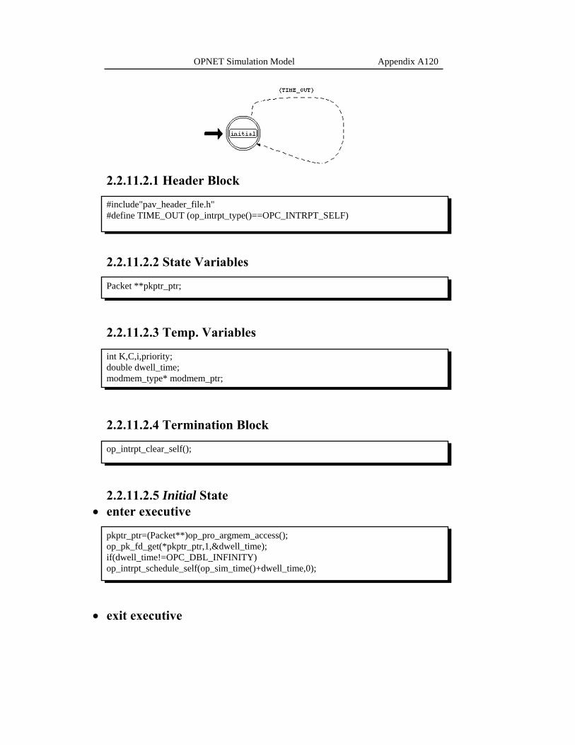
120 OPNET Simulation Model Appendix A
2.2.11.2.1 Header Block #include"pav_header_file.h" #define TIME_OUT (op_intrpt_type()==OPC_INTRPT_SELF) 2.2.11.2.2 State Variables Packet **pkptr_ptr; 2.2.11.2.3 Temp. Variables int K,C,i,priority; double dwell_time; modmem_type* modmem_ptr; 2.2.11.2.4 Termination Block op_intrpt_clear_self(); 2.2.11.2.5 Initial State
• enter executive pkptr_ptr=(Packet**)op_pro_argmem_access(); op_pk_fd_get(*pkptr_ptr,1,&dwell_time); if(dwell_time!=OPC_DBL_INFINITY) op_intrpt_schedule_self(op_sim_time()+dwell_time,0);
• exit executive
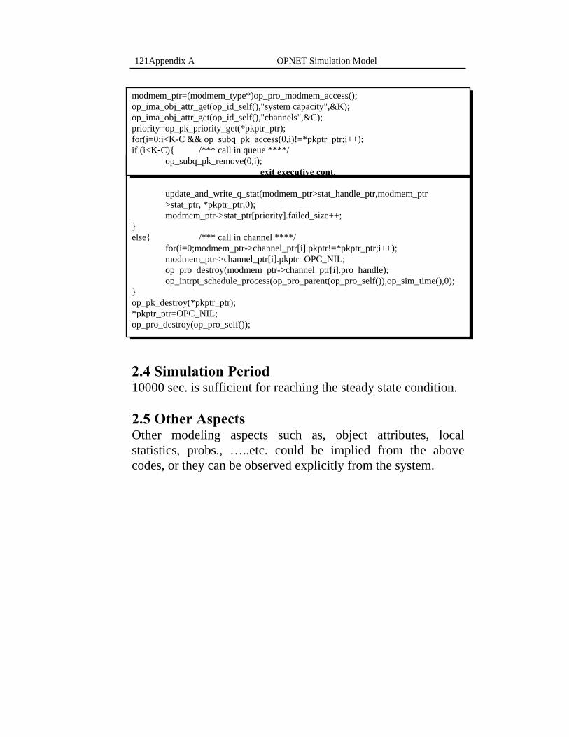
Appendix A OPNET Simulation Model 121
modmem_ptr=(modmem_type*)op_pro_modmem_access(); op_ima_obj_attr_get(op_id_self(),"system capacity",&K); op_ima_obj_attr_get(op_id_self(),"channels",&C); priority=op_pk_priority_get(*pkptr_ptr); for(i=0;i<K-C && op_subq_pk_access(0,i)!=*pkptr_ptr;i++); if (i<K-C){ /*** call in queue ****/
op_subq_pk_remove(0,i); exit executive cont.
update_and_write_q_stat(modmem_ptr>stat_handle_ptr,modmem_ptr
>stat_ptr, *pkptr_ptr,0); modmem_ptr->stat_ptr[priority].failed_size++; } else{ /*** call in channel ****/ for(i=0;modmem_ptr->channel_ptr[i].pkptr!=*pkptr_ptr;i++); modmem_ptr->channel_ptr[i].pkptr=OPC_NIL; op_pro_destroy(modmem_ptr->channel_ptr[i].pro_handle);
op_intrpt_schedule_process(op_pro_parent(op_pro_self()),op_sim_time(),0); } op_pk_destroy(*pkptr_ptr); *pkptr_ptr=OPC_NIL; op_pro_destroy(op_pro_self());
2.4 Simulation Period 10000 sec. is sufficient for reaching the steady state condition. 2.5 Other Aspects Other modeling aspects such as, object attributes, local statistics, probs., …..etc. could be implied from the above codes, or they can be observed explicitly from the system.
References
[1]Asha Mehrotra, “Cellular Radio, Analogue and Digital
Sytems”, 1994. [2]Berruto, G. Colombo, P. Monogiousdis, A. Napolitano, K.
Sabatakakis, “Architectural Aspects for the Evolution of Mobile Communications Toward UMTS”, IEEE Journal on selected areas in Communications, vol. 15, No. 8, Oct. 1997.
[3]Computer Technology Research Corp., “Computer
Telephony and Wireless Technologies”, 1997 [4]David J. Goodman, “ Wireless Personal Communications
Systems”, 1997. [5]Donald Gross, Carl M. Harris, “Fundamentals of queueing
theory”, 1985. [6]Fred j. Ricci, “Personal Communications Systems
Applications”, 1997. [7]Intel Corporation, GSM Data Knowledge Site:
“http://www.gsmdata.com/whatsgsm.htm”, 1998. [8]Lawrence Harte, Richard Levine, Steve Prokup, “Cellular
and PCS, The Big Picture”, 1997. [9]MIL 3, Inc., OPNET/MODELER manuals, vol. 1, vol. 2,
vol. 3, vol. 6, vol. 7, vol. 8, 1997.
References 123
[10]Pavlidou, “Two dimensional traffic models for cellular mobile systems”, IEEE trans. Commun., vol. 42, pp. 1505-1511, Feb./Mar./Apr. 1994.
[11]Bennett, “Simulation Fundamentals”, 1995. [12]Stephen Wolfram, “Mathematica: a System for Doing
Mathematics by Computer”, 1988. [13]Stewart Robinson, “Successful Simulation”, 1994. [14]Thomas B. Bahder, “Mathematica for Scientists and
Engineers”, 1995. [15]Uddenfeldt, “Digital Cellular- Its Roots and Its Future”,
IEEE Proc., vol. 86, No. 7, Jul. 1998. [16]William C. Y. Lee, “Mobile Cellular Telecommunications,
Analogue and Digital Systems”, 1995. [17]Z. Mohasseb, “Prioritized channel assignment in cellular
radio networks”, Thesis of M.Sc. degree, Military Technical College, Egypt, 1996