Simulation of Pressure- and Tube-tooling Wire-Coating Flowsthrough DistributedComputation

A. BALOCH, H. MATALLAH, V. NGAMARAMVARANGGUL‡

AND

M. F. WEBSTER*

Institute of Non-Newtonian Fluid Mechanics,Department of Computer Science,

University of Wales, Swansea, SA2 8PP, UK.

‡Faculty of Science, Chulalongkorn University, Thailand

Int. J. Num. Meth. Heat & Fluid Flow, 6 March 2002

SUMMARY

This article focuses on the comparative study of annular wire-coating flows with polymermelt materials. Different process designs are considered of pressure- and tube-tooling,complementing earlier studies on individual designs. A novel mass-balance free-surfacelocation technique is proposed. The polymeric materials are represented via shear-thinning, differential viscoelastic constitutive models, taken of exponential Phan-Thien/Tanner form. Simulations are conducted for these industrial problems throughdistributed parallel computation, using a semi-implicit time-stepping Taylor-Galerkin/pressure-correction algorithm. On typical field results and by comparing short-against full-die pressure-tooling solutions, shear-rates are observed to increase ten fold,while strain rates increase one hundred times. Tube-tooling shear and extension-rates areone quarter of those for pressure-tooling. These findings across design options, haveconsiderable bearing on the appropriateness of choice for the respective process involved.Parallel finite element results are generated on a homogeneous network of Intel-chipworkstations, running PVM (Parallel Vitual Machine) protocol over a Solaris operatingsystem. Parallel timings yield practically ideal linear speed-up over the set number ofprocessors.

Keywords: Polymer Melts, Viscoelastic Fluids, Wire-Coating Flow, Pressure-Tooling,Tube-Tooling, Drag Flow, Parallel Computation, PVM, Finite Element Method

* Author for correspondence• Supported by a grant from the UK EPSRC GR/L14916

2

1. INTRODUCTION

A number of highly viscoelastic, complex extrusion flows are investigated, commonlyassociated with the coatings of glass rovings, fibre-optic cables, wire and cablemanufacturing processes. Three flow problems are considered, die swell/drag flow (short-die pressure-tooling), full pressure-tooling, and tube-tooling flow. The first two cases aresuitable for simulating industrial narrow-bore wire-coating processes. Tube-tooling dealswith thicker (wide-bore) wire-coating processes. To provide realistic flow representationfor the polymer melt materials used in practice, the specific choice is made of aviscoelastic constitutive model to support shear-thinning and strain-softening behaviour.To this end, an exponential Phan-Thien/Tanner (EPTT) model is selected, flows arecomputed in a two-dimensional annular coordinate system under creeping flowconditions, and a parallelised version of a semi-implicit time-marching finite elementscheme is used, Taylor-Galerkin/pressure-correction (TGPC).

Wire-coating has been studied extensively in experimental and computational form overrecent years, see [1] for review. Most studies concentrate on the pressure-tooling design.Modelling assumptions commonly include isothermal flow conditions, incompressibilityof the coating flow [2], concentricity of the wire [3], and wire speeds ranging up to onemeter per second [4]. Wire-coating, in the pressure-tooling context, constitutes a processof two flow regimes: a shear dominated flow within an annular die, and an extension-dominated flow along the wire-coating region beyond the die. Injection of the moltenpolymer into the tooling die establishes a pressure-driven flow. Contact between themolten plastic tube and the wire is made within the die for pressure-tooling, where thetravelling wire induces a drag flow, drawing out the polymer melt to form a sheath aroundthe cable. Unique to tube-tooling design is the dependency upon the effects of draw-downbeyond the die. Coating production lines for narrow-bore wire use relatively high speeds,around one meter per second, and the deposition of the fluid on a rigid moving wire istreated as a free surface problem.

Recent attention by a number of authors has focused on the simulation of pressure-toolingflow for viscous fluids, such as those of Caswell and Tanner [5], Pittman and Rashid [6],Mitsoulis [7], Mitsoulis et al. [8], and Wagner and Mitsoulis [9]. Their work dealt mainlywith shear flow under both isothermal and non-isothermal conditions. Molten polymershave been noted to exhibit highly elastic behaviour when subject to large deformation[10]. Only recently, numerical techniques have proven capable of reaching solutions forsufficiently high and relevant levels of elasticity. Many attempts involving eitherlubrication or inelastic approximations have been conducted to addressed theseshortcomings [5,8,11]. With finite elements (FE), Mitsoulis [7] studied the wire-coatingflow of power-law and Newtonian fluids. Mitsoulis concluded that the inclusion of shear-thinning reduced the levels of die-swell at the die-exit, as well as the recirculation thatoccurred within the die. In a subsequent article, Mitsoulis et al. [8] provided a detailedinvestigation into high-speed industrial wire-coating. Two flow formulations were used; aplanar FE analysis for non-isothermal flows, and a lubrication approximation forisothermal, power-law fluids. Results corroborated the experimental findings of Haas andKewis [12].

The inadequacy of inelastic modelling was made apparent by Binding et al. [13], rediscrepancies in stress and pressure drop. To predict residual stressing within the meltcoating, a viscoelastic analysis was recommended to account for the influence of short

3

residence times of the particles within the flow. Hence, we have adopted differentialviscoelastic models, to predict stress development, using state-of-the-art FE techniques toreach the high deformation rates encountered and associated high Weissenberg numbers,O(104). For tube-tooling flows and fixed free-surface estimation, we have conductedsingle-mode PTT (Phan-Thien/Tanner) simulations in Mutlu et al. [4,14] and Matallah etal. [10]. Tube-tooling was analysed in sections in Mutlu et al. [4], isolating draw-downflow and studying the effects of stress pre-history and various boundary conditions. Thisled to a further study [14] on coupled and decoupled solution procedures for a range ofmodel fluids, approaching those of industrial relevance. In Matallah et al. [10], single-mode calculations were compared to those of multi-mode type for LDPE and HDPE gradepolymers. The multi-mode computations revealed the dominant modes of mostsignificance to the process and gave insight as to the levels of residual stress in theresultant coatings. Further work on multi-mode modelling of Matallah et al. [15],emphasised the influence of die-design on optimal process setting. Three, as opposed toseven modes, were found adequate to sufficiently describe the flow. The draw-downresidence time, which dictates the dominance of certain modes within the relaxation timespectrum, was found to be a major factor to influence the decay of residual stressing in thecoating.

With specific attention paid to slip for viscous flows, a semi-implicit Taylor-Galerkin/pressure-correction procedure was used by the present authors [16] for pressure-tooling and tube-tooling. There, the influence of slip onset, as opposed to no-slipconditions within the die, was examined. Tracking free surfaces, our earlier work onmodel problems addressed stick-slip and die-swell flows, see References [17,18]. In arecent article for pressure-tooling [1], the influence of material rheology was investigatedon free-surface flow, whilst tube-tooling was the subject in Reference [10]. The presentanalysis extends upon this work, contrasting comparative designs via a distributed parallelimplementation. The computational efficiency over various processor-cluster sizes is ofparticular interest. Distributed computations are performed over homogeneous networkclusters of Intel-chip workstations, running a Solaris Operating System. In this respect,our earlier experience with parallelisation for large, yet model problems [19], is taken intothe industrial processing realm. There, Parallel Virtual Machine (PVM) message passinglibraries were used over heterogeneous clusters, comprising of DEC-alpha, Intel-Solarisand AMD-K7 (Athlon) Linux processors.

The outline of the current paper is as follows. First, the governing equations are described,followed by the rheological behaviour of the PTT model. In section 4, the three differentproblems are specified. This is followed, by an outline to the parallel TGPC numericalmethod employed for the simulations. The results of the simulations are presented insection 6 and some conclusions are drawn in section 7.

2. GOVERNING EQUATIONS

Isothermal flow of incompressible viscoelastic fluid can be modelled through a systemcomprising of the generalised momentum transport, conservation of mass and viscoelasticstress constitutive equations. The problems in this study are modeled as annular and two-dimensional. In the absence of body forces, such a system can be represented in the form:

∇ =.v 0, (1)

ρ ρ∂

∂= ∇ − ∇v

v vt

. .σ . (2)

4

Here, v is the fluid velocity vector field, σ is the Cauchy stress tensor, ρ is the fluiddensity, t represents time, and divergence and gradient operations are implied via ∇ . TheCauchy stress tensor can be expressed in the form:

σ = - pδ + Te,

where p is the isotropic fluid pressure, δ is the Kronecker delta tensor, and Te is the stresstensor. For viscoelastic flows, stress Te can be decomposed into solvent and polymericcontributions,

Te = τ + 2µ2d,

with tensors, τ, the elastic extra-stress and rate-of-strain d=0 5. [ ( ]∇ + ∇v v †) (superscript †

denotes a matrix transpose). µ2 is a solvent and µ1 a polymeric solute viscosity, such thatµ = µ 1 + µ 2. The particular choice of constitutive model is that of Phan-Thien/Tanner[20,21], in exponential form (EPPT). In contrast to models, such as constant shearviscosity Oldroyd-B, this EPPT version supports shear-thinning and finite extensionalviscosity behaviour. The constitutive equations for the extra-stress of the EPTT model isexpressed as:

λ µ λ1 1 12

∂∂

= + ∇ + ∇ ∇{ }τ τ τ τ τt

(d v v vf - . - .†

) . , (3)

with an averaged relaxation time λ1 and function f, defined in terms of trace of stress,trace(τ ), as:

f = exp[ ( )]ελ

µ τ1

1

trace .

The material parameters that control shear and elongational properties of the fluid are εand µ1, respectively. These may be evaluated by fitting to the experimental data [10,15].When ε vanishes, the Oldroyd-B model is recovered and f=1.

We find it convenient to express the governing equations in non-dimensional form, bydefining corresponding scales of characteristic length R, taken as coating length (figures2-4), and wire-speed as characteristic velocity scale, V. Then, stress and pressure are

scaled by a factor of R

Vµ , and time by VR . There are two non-dimensional group numbers

of relevance, Weissenberg number We VR= λ 1 and Reynolds number

Re VR= ρµ .

3. SHEAR AND ELONGATIONAL BEHAVIOUR OF EPTT

Many common non-Newtonian fluids exhibit non-constant viscosity behaviour. So, forexample, such materials may display shear-thinning, where the viscosity is a decreasingfunction of increasing shear rate as illustrated in Figures 1a in pure shear. Figure 1breflects a similar plot, demonstrating the functional dependence of viscosity underincreasing strain-rate in pure uniaxial extension. This is termed the elongational orextensional viscosity behaviour. The merits of the PTT model over the Maxwell model arehighlighted by Phan-Thien/Tanner [22], noting that, the Maxwellian elongationalviscosity is singular at finite strain rates. The shear and extensional viscosity functions, µs

5

and µe, of the PTT model variants may be expressed as a function of f itself, taken ofexponential form as above, via

µ γ µ µ

s(˙) = +21

f, (4)

and

µ ε µ µ

λ εµ

λ εe(˙) ˙ ˙= +

−+

+3

222

1

1

1

1f f. (5)

Under general flow conditions, there is need to record generalized shear and strain-rates,that are defined via flow invariants as, respectively:

γ̇ =2 IId , ε̇ = 3IIIII

d

d

, (6)

where IId and IIId are the second and third invariants of the rate of strain tensor d. Suchquantities are represented as

II trace

r z r z rdr z r r z= = ∂

∂+ ∂

∂+ + ∂

∂+ ∂

∂12

12

12

2 2 2 2( ) {( ) ( ) ( ) ( ) }dv v v v v

, (7)

III et

r r z z rdr r z r z= = ∂

∂∂∂

− ∂∂

+ ∂∂

d ( ) { ( ) }dv v v v v1

42

. (8)

In pure shear, µs varies with ε, µ1, and λ1. The effect of elevating µ1 from levels of 0.88 to0.99 and 0.95 reduces the second Newtonian plateau level from 0(10-1) to 0(10-2) andbelow. Here, µ1 = 0.99 solute fraction is taken as suitable. Shifting of λ1, (via We) fromunity to 0(10) and 0(102), translates µs in a constant shift fashion. The larger λ1, the earlierthe departure occurs from the first Newtonian plateau. Current material and processsettings suggest λ1 of 0(1s) is a reasonable choice, so that We=200. With selection of µ1 =0.99 and We=200, the influence of the ε-parameter choice is relatively minor. Increasing εfrom 0.1 to 0(1) slightly retards the µs pattern, so that earlier departure from the firstNewtonian plateau occurs. Here, ε of unity is selected.

In steady uniaxial extension, µe follows the behavioural trends of µs for both We and µ1

parameters. Distinction may be found via the ε-parameter. Taking the tuple setting (µ1,

We) = (0.99,200), for 0.1≤ε ≤0.5, reflects strain-hardening at low strain rates prior tosoftening at rates above 10-2. Only softening is apparent for ε~0(1). The EPTT(1,0.99,200) model demonstrates the desired viscometric functional behaviour, shear-thinning and strain-softening, within the deformation rate ranges of dominant interest forthe wire-coating process, as one might typically encounter, say, for an LDPE gradepolymer at 230oC. As a consequence of these viscometric functions, we observe later inthe actual flows of current interest, that maximum shear-rates may rise to O(102) units,whilst strain-rates reach O(101). This, in turn, implies that second Newtonian plateaus willbe reached in-situ.

4. SPECIFICATION OF PROBLEMS

This paper deals with the study of three types of flow: die swell/drag flow (short-dietooling), full-die pressure-tooling flow, and tube-tooling flow.

6

4.1 Die-Swell/Drag Flow

This annular problem illustrates the progressive effects of an imposed drag flow from thetravelling wire on both the classic die swell problem (within the free jet-flow region) andstick-slip flow (see Figure 2). Mesh refinement considerations follow our previous studies[1,17,18], where the fine mesh of Figure 2b is found suitable. The flowrate through the dieis fixed by the fully-developed annular inlet flow profile under pressure-driven conditions.No-slip conditions are applied at the die wall boundaries. The wire and inlet channel radiicomprise the characteristic length, while characteristic velocity is directly related to theconstant wire-speed at the lower boundary of the domain. The rapid reduction in tractionat the free jet surface gives rise to the fully-developed plug flow at the domain outflow.

4.2 Pressure-Tooling

Pressure-tooling flow is an extension to the previous die-swell/drag flow study, thedomain of which is specified in Figure 3a. This domain contains an initial short-die flowzone within the land region of the die (z6, z7), followed by a jet flow region at the die exit.The traveling wire within the die, moving at a fixed speed, first makes contact with thepressure-driven annular flow at z3 station. The influence of the wire on the polymer meltat this boundary region is referred to in references [1,13,16]. Flow within the die isrestrained by no-slip boundary conditions at the die walls. The swelling effects observedin the jet flow region are caused by the sudden drop to atmospheric pressure, combinedwith the immediate lack of traction. This swell, in the extruded polymer, levels out to afully-developed plug flow, by the time it reaches the end of the pressure-tooling domain.The biased fine mesh of Figure 3b is employed, for further details see our prior study [1].

4.3 Tube-Tooling

A schematic illustration of the full-die tube-tooling domain is shown in Figure 4a. Thiswas computed upon with the fine mesh of Figure 4b. Problem dimensions are largely incommon with the full pressure-tooling specification. So, for example, the lower and upperdie wall converging angles are 30o and 17o, at positions z10 and z3, respectively. No-slipdie-wall boundary conditions apply throughout the die. In the final draw-down region(z4z5 and z8z9), free surface conditions apply. For tube-tooling, the wire makes contactwith the polymer melt at the end of the draw-down region z5, with the coating length uponthe wire being taken as the characteristic length R2. As for pressure-tooling, the wiredimensions, inlet hydraulic radius (R2), and total die length (3R2), again apply in thisexample. In our previous investigations [1,18], we focused upon mesh convergencestudies. Here, numerical solutions are generated on fine meshes only, the detailed statisticsof which are recorded in Table 1 for all three problems, inclusive of degrees of freedom(DOF), for Newtonian (N) models and viscoelastic (V) models.

Meshes Elements Nodes DOF(N) DOF(V)Short-Die 288 377 929 2437Pressure-Tooling 3810 7905 17858 49478Tube-Tooling 4714 9755 22031 61051

Table 1: Finite Element Mesh Data

7

Sub-region zoneBiased

fine mesh

1. inlet die 15×20

2. converging die 15×25

3. coating region 15×30

4. land region 15×5

5. jet region 15×47

Table 2a: Full-die pressure-tooling; mesh characteristics, sub-region zones

Sub-region zoneBiased fine

mesh

1. inlet die 12×45

2. converging die 12×18 + 15×8

3. land region 15×12 + 20×12

4. draw-down region 20×25

5. coating region 20×25

Table 2b: Tube-tooling; mesh characteristics, sub-region zones

5. NUMERICAL SCHEME

5.1 Sequential Taylor-Galerkin Algorithm

A time-marching finite element algorithm is employed in this investigation to computesteady viscoelastic solutions through a semi-implicit Taylor-Petrov-Galerkin/pressure-correction scheme [23-28], based on a fractional-step formulation. This involvesdiscretisation for equations (1-3), first in the temporal domain, adopting a Taylor seriesexpansion in time and a pressure-correction operator-split, to build a second-order time-stepping scheme. Spatial discretisation is achieved via Galerkin approximation formomentum and Petrov-Galerkin for the constitutive equations. The finite element basisfunctions employed are quadratic for velocities and stress, and linear for pressure, definedover two-dimensional triangular elements. Galerkin integrals are evaluated by a sevenpoint Gauss quadrature rule. The time-stepping scheme includes a semi-implicit treatmentfor the momentum equation to avoid restrictive viscous stability constraints. Solution ofeach fractional-staged equation is accomplished via an iterative solver. That is, with theexception of the temporal pressure-difference Poisson equation, which is solved through adirect Choleski procedure. The semi-implicit Taylor-Galerkin/pressure-correction methodmay be presented in semi-discrete temporal format as:

8

Stage 1a:

2 nReRe n n

∆t( pn nv v d v v d d+ +− = ∇ ⋅ + − ⋅ ∇ − ∇ + ∇ ⋅ −

12

122 2 2) ( ) ] ( )[ µ µτ ,

21

WeWe

∆tfn n n( ) 2τ τ τ τ τ τ+ − = − − ⋅ ∇ − ∇ ⋅ − ∇ ⋅

12 µ d v v v[ ( ) ]†

.

Stage 1b:

ReRe

∆t( pn n n nv v d v v d d* *) ( ] [ ] ( )− = ∇ ⋅ − ∇ + ∇ ⋅ − ⋅ ∇ + ∇ ⋅ −+[ 2 2 2

12µ µτ ,

WeWe

∆tfn n n( ) 2τ τ τ τ τ τ+ +− = − − ⋅ ∇ − ∇ ⋅ − ∇ ⋅

12

12µ1d v v v[ ( ) ]†.

Stage 2:

∆tp pn n

22∇ − = ∇ ⋅+( )1 Re v*

.

Stage 3:

2Re∆t

pn n( v v+ +− = −∇1 1* ) ( - p )n.

Here, n is the time step number and v* is a non-solenoidal vector field. The velocity andstress components of Stage 1a are taken for a half time step (i.e., n+ 2

1 ), while at Stage 1b,the v* velocities and stresses are computed over a full time step (n+1). In combination,Stage 1 constitutes a predictor-corrector doublet, performed once per time-step. Thisconcludes derivation of stress components for a complete time step. Pressure differencesover this period are calculated from the Poisson equation (Stage 2), depending upon theintermediate vector field v*. Solution of this Poisson equation yields the solenoidalvelocity over a full time step, as shown in Stage 3 (see [23,24]). Free-surface reassessmentis conducted at a fourth stage (see on). Recovery of velocity gradients within theconstitutive equation further enhances stability of the system, along with streamline-upwind Petrov-Galerkin weighting. Determination of time step (typically O(10-3)) is madeon the basis of a Courant stability constraint.

5.2 Parallel Taylor-Galerkin Algorithm

The semi-implicit time-stepping TGPC algorithm is parallelised as follows. Each of theindividual fractional-stage phases of the algorithm is parallelised within a single time-steploop. This implies operations of gather and scatter of data, pre- and post- each phase,respectively. In such a manner, the combined problem is split into associated sub-problems relating to each subdomain. We relate such operations with message passingbetween master and slave processors, achieved via PVM send and receive communicationcommands. This is a crucial issue to ensure correct system configuration and networkcommunication. The slave processors solve subdomain problems, whilst the masterprocessor resolves the interface problem and controls master-slave communication [29].

Of the various fractional-stages, the pressure equation step is the only one that isconducted through a direct solution procedure (Choleski), involving the explicit parallelconstruction and solution of a matrix problem. Remaining stages are associated with aniterative solution procedure (Jacobi). It is upon this basis that the exceptional parallelperformance characteristics are achieved. The complete detail behind the parallelisation of

9

the TGPC and these two algebraic solution procedures is provided in [29]. Briefly, bothnecessitate an assembly and solution phase, involving finite element loop construction ofright-hand-side vectors and matrix components. For Choleski, the matrix componentsmust be stored. Fortunately, this is manageable even for large problems, as the pressurevariable in question is of scalar form on the field.

Solution phases radically differ between iterative and direct procedures. The iterativesolution phase is nodally-based. Each sub-problem on a slave processor, first computescontributions for the boundary (interfacing) nodes, so that their result may becommunicated to the master processor directly, whilst the computation for interior sub-domain nodes is completed. This enables effective masking of communication. Themaster processor must then process the combined domain contributions for the interfacingnodes, as well as performing system synchronisation and intercommunication processorcontrol. Utilising an iteration number r, acceleration factor ω, right-hand side vector b,iteration sub-domain vector XPi, system (mass) matrix Mfe and diagonal matrix Md, theparallel finite element Jacobi iteration may be expressed in concise notational form, as

nodes1

d

r

nodesP

P

P

P

fe1

d

1r

nodesP

P

P

P

]b[M

X......

...

X...

X...

X

)MMI(

X.........

X...

X...

X

par

n

3

2

1

n

3

2

1

−−

+

ω+

ω−=

The mass-matrix (Mfe) is based on quadratic finite element functions, its diagonalisedform (Md) is one of absolute row-sum, and the iterative acceleration parameter ω may beselected to suit (often simply taken as unity). System matrices are referenced andevaluated at the element level only, so that a complete system is never stored. A singleiteration sweep of this sort will maintain integrity levels of the data re-synchronisation.Care likewise must be taken with respect to consistent solution increment tolerancecalculations, across individual slave and master processors.

The parallel direct solution phase adopts a Schur-complement approach. This introduces aherring-bone structure to the complete system matrix problem, via the associated nodalnumbering on each subdomain and the interfacing boundary nodes. The parallel herring-bone structure of the Choleski system matrix may be represented as

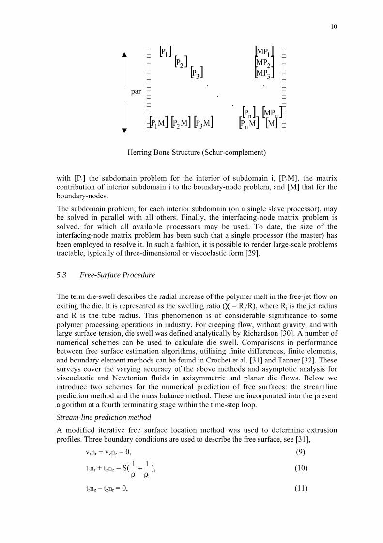
10

par

[ ][ ]

[ ][ ][ ][ ]

[ ] [ ] [ ][ ] [ ]

[ ] [ ]

MMPMPP

.

MPMPMP

..

MPMPMP

.P

PP

n

nn

321

3

2

1

3

2

1

Herring Bone Structure (Schur-complement)

with [Pi] the subdomain problem for the interior of subdomain i, [PiM], the matrixcontribution of interior subdomain i to the boundary-node problem, and [M] that for theboundary-nodes.

The subdomain problem, for each interior subdomain (on a single slave processor), maybe solved in parallel with all others. Finally, the interfacing-node matrix problem issolved, for which all available processors may be used. To date, the size of theinterfacing-node matrix problem has been such that a single processor (the master) hasbeen employed to resolve it. In such a fashion, it is possible to render large-scale problemstractable, typically of three-dimensional or viscoelastic form [29].

5.3 Free-Surface Procedure

The term die-swell describes the radial increase of the polymer melt in the free-jet flow onexiting the die. It is represented as the swelling ratio (χ = Rj/R), where Rj is the jet radiusand R is the tube radius. This phenomenon is of considerable significance to somepolymer processing operations in industry. For creeping flow, without gravity, and withlarge surface tension, die swell was defined analytically by Richardson [30]. A number ofnumerical schemes can be used to calculate die swell. Comparisons in performancebetween free surface estimation algorithms, utilising finite differences, finite elements,and boundary element methods can be found in Crochet et al. [31] and Tanner [32]. Thesesurveys cover the varying accuracy of the above methods and asymptotic analysis forviscoelastic and Newtonian fluids in axisymmetric and planar die flows. Below weintroduce two schemes for the numerical prediction of free surfaces: the streamlineprediction method and the mass balance method. These are incorporated into the presentalgorithm at a fourth terminating stage within the time-step loop.

Stream-line prediction method

A modified iterative free surface location method was used to determine extrusionprofiles. Three boundary conditions are used to describe the free surface, see [31],

vrnr + vznz = 0, (9)

trnr + tznz = S( 1 1

1 2ρ ρ+ ), (10)

trnz – tznr = 0, (11)

11

where free surface unit normal components are (nr, nz), curvature radii (ρ1, ρ2), surfacetension coefficient S (vanishes here), radial and axial velocities (vr, vz) and surface forcesnormal to the free surface (tr, tz).

Boundary condition (10) and (11) are used when iteratively modelling the free surface.Conditions (9) is then included to define the normal velocity. The upper extruded flowsurface can then be obtained for die-swell extrusion. For a tube radius R, the distance r(z)of the free surface from the axis of symmetry is represented by:

r z R

zz

dzr

zz

( )( )( )

= +=

∞∫ vv0

. (12)

In order to accurately predict the extrusion shape, Simpsons quadrature rule is used tocompute the integral of equation (12).

The procedure of solution is as follows. First, the kinematics for a converged Newtoniansolution is used as initial conditions, with a relaxed stress field, and the fixed free-surfaceproblem is solved. Subsequently, the full problem is computed, involving the free surfacecalculation, where the surface location itself must be determined. Continuation from oneparticular viscoelastic solution setting to the next is then employed. In some instances, it isstabilising to first enforce vanishing surface extra-stress (τ of equation (3)), prior torelaxing such a constraint. To satisfy the zero normal velocity free surface boundarycondition and to compensate for the adjustment of the free surface, the velocity solution atthe advanced time surface position must be reprojected from the previous surface position.

Mass balance method

The pressure drop/mass balance method provides an adequate means of correcting theestimation of the free surface position. Such a technique may provide improved solutionaccuracy and stability over the regular streamline location method. The procedureinvolves taking, an initial estimate of the free-surface profile for each Weissenbergnumber. Sampling points for We begin from the stick-slip region. The final correctionstage makes use of the streamline method, to perturb and validate the position of the dieswell surface.

By examining the functional dependence of pressure drop ( ∆p) on swell (χ) profiles atthe centreline, for each We level, the mass balance scheme relates flow characteristicsbetween the stick-slip to die-swell phases of the problem (akin to an expression of energybalance). By taking into account known swell predictions with sampled pressure dropresults, a general relationship may be established between these two scenarios:

χ( )( , )( )

zp z Wef We

= ∆,

By fitting to prior and accepted data (say at low We levels, from the streamline method),the denominator can be represented by:

f(We) = 10.68 - 0.133We - 2.425We2.

Using this approach, it is possible to derive the approximate swell after pressure dropcalculations are made. This process is then implemented within an iterative time-steppingprocedure, to obtain a converged solution. Such a strategy is found to be absolutelynecessary to achieve converged free-surface solutions at the extreme levels of parametersrelevant to industrial processing, notably high We and low solvent contribution.

12

6. NUMERICAL PREDICTIONS AND DISCUSSION

6.1 Short-die, pressure-tooling

The solution for short-die pressure-tooling is illustrated through field plots, in terms ofpressure, extension rate and shear rate in Figure 5 and stress component contours in Figure7. The short-die problem, taken on the 6x24 element mesh, is an idealised flow. It provesuseful to encapsulate the essence of pressure-tooling, devoid of the complexity of the fulldie. In contrast, the full-die study reveals the implications of actual processing conditions.

The pressure drop across the flow reaches 0.46 units (relative to ambient pressure), wherethe die length to exit gap width ratio is of the order 2:1. This drop corresponds to thatacross the die alone. The minimum pressure arises at the top surface die-exit. The shearrate I2 is two orders of magnitude larger than the extension rate, peaking with 31.3 units atthe top die-exit boundary. Upon entering the jet region, the shear rate rapidly declines andvanishes. The flow profile adjusts from a shear flow within the die to a plug flow in thejet. The flow profiles of Figure 6 reflect this position, with a linear decrease in pressureobserved along the wire within the die. Maximum swell within the jet reaches 1.054 units.This would correspond to typical results reported in the literature [7-9, 17, 18].

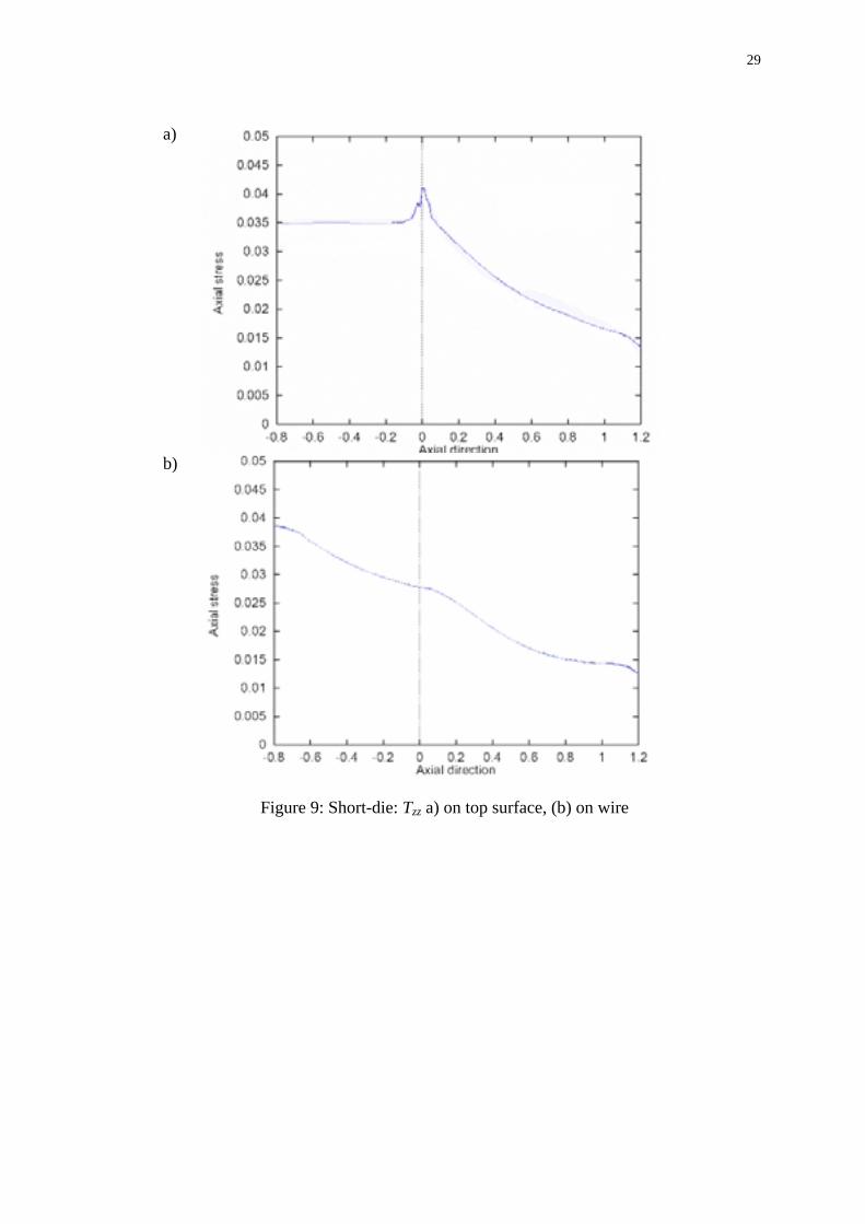
Field plots on the stress components of Figure 7, illustrate the dominance of the axialstress, that in maxima is three times larger than the shear stress and five times larger thanthe radial stress. The sharp adjustment is noted at die-exit on the top-surface in both shearand axial stress, Trz and Tzz-profiles of Figure 8 and 9, respectively. Profiles on the wireare relatively smooth, in contrast. We have observed in our earlier work [1], that thestrain-softening response of the EPTT model, stabilises stress profiles. This stands in starkcontrast to models that support strain-hardening.

6.2 Full-die, pressure-tooling

Following our earlier study on mesh convergence [1], for this problem our results areplotted upon the biased fine mesh of Figure 3b, with identical parameter settings as for theshort-die flow. The zonal refinements are outlined in Table 2a, with greatest density andbias in the land and die-exit regions.

The field plots of Figure 10 Indicate an intense drop in pressure local to the land region,reaching a maximum pressure drop of 10.1 units. Shear rate, I2, also identifies significantshearing over the land region, reaching a peak of 461 units at the die-exit, a fifteen foldincrease to that obtained for short-die tooling. Strain rates, ε̇, are an order of magnitudelower than shear rates, and display peaks at melt-wire contact and die-exit. At the melt-wire contact point, ε̇ increases to 8.37 units. A rapid larger rise occurs in the wire-coatingsection at die-exit. The second peak in ε̇-profile at the top boundary, characteristic for thefull-die, reaches a height of 18.8 units in the post-die exit region.

The pressure along the bottom surface corresponds to the line contour plot of Figure 11a.Pressure difference is twenty two times greater for the full case, above short-die pressure-tooling (as compared with Figure 5). Note that, these drops in pressure, essentiallycorrespond to the same flow zone, that is, over the land-region at jet-entry. The die-swellprofile along the top free-surface is given in Figure 11b. The swelling ratio is fifteenpercent larger than that for short-die pressure-tooling.

13

Solutionvariables

Short-die Full-die Tube-tooling

I2 max, Top 31.35 461.7 127.2

I2 max, Bot -- 139.7 144.2

ε̇ max 0.144 18.83 4.43

∆p 0.462 10.18 16.09

Trz max 0.014 0.025 0.024

Tzz max 0.041 0.069 0.050

χ 1.054 1.215 ---

Table 3: EPTT(ε=1, µ1=0.99, We=200), solution values

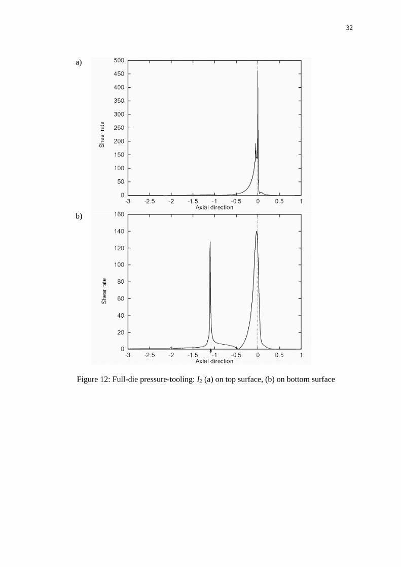
Shear rate profiles, along the top and bottom surfaces, are represented in Figure 12. Thetop surface I2 peak of 461.7 units at the die-exit (Figure 12a), is fifteen times greater thanthat for short-die, pressure-tooling (see Figure 6b). Further data on I2 maxima may befound in Table 3. Along the bottom surface, the double (sudden shock) peaks of 124 and140 units of Figure 12b are most prominent. Such peaks do not appear in the short-diecase, being a new introduction as a consequence of the full-die and melt-wire contact.

The “shock impact” as the fluid makes contact with the wire is most prominent in theradial, shear and axial stress contour plots of Figure 13. Nevertheless, stress levels withinthe die remain small, the greatest axial stress of 0.069 units occurs upon melt-wire contact.

Top-surface stress profiles of Figures 14a and 15a, demonstrate most clearly, the“localised effect” of die-exit point discontinuity. A violent jump in shear stress isobserved over the land region. Comparison of stress between full-die and short-diepressure-tooling instances reveals factor increases of 1.8 times in Trz and 1.7 times in Tzz

(Table 3). Both shear and axial stress profiles along the bottom wire-surface reveal theinfluence of the moving-wire on the flow at the melt-wire contact point (axial position–1.1 units). In axial stress of Figure 15, along the bottom surface, the characteristic“double peak” profile at the melt-wire contact point and die-exit regions is observed. Theaxial stress peak at the melt-wire contact point exceeds that at die-exit and is followed bya sharp relaxation on the approach to the land region, upon which a more sustainedmaxima forms. Notably, in the extrudate, Tzz remains positive, and provides some residualstressing to the coating. Tzz-maxima increase only slightly from case to case, with full-casepressure-tooling values being about twice those for the short-die instance.

6.3 Tube-tooling

Concerning the tube-tooling problem, our analyses are based on a single refined mesh asdisplayed in Figure 4b, see Ref. 33. Mesh characteristics for each sub-region are providedin Table 2b. As displayed in Figure 16a, the pressure-drop is most prominent across thetube-die. At the draw-down and coating regions, the pressure holds to an ambient level.The most important rate of change in pressure-drop arises across the land-region, as is truefor pressure-tooling. Here, the maximum value is higher, of 16.1 units for tube-toolingcompared to 10.2 units for pressure-tooling.

In contrast, shear-rate I2, is about a quarter of that corresponding to pressure-tooling. Themaximum is 144 units. Again, higher shear-rates are attained in the land-region, see

14

Figure 16b. The remaining regions display smaller shear-rates, so that the shear-viscosityof the polymer melt will be high there. The shear-rate profiles are also displayed in Figure17b and c, plotted along the top and bottom surfaces in the axial direction. The shear-ratesincrease across the converging cone, from 0.89 units at the inlet-tube and start of theconverging cone to 14.6 units at its end. A sudden rise in shear-rate occurs when thepolymer enters the land-region, across which a constant value is generated. Shear-ratemaxima are generated at the die-exit, with values of 144.2 and 127.2 units at the bottomand top surfaces, respectively. Beyond the die-exit entering the draw-down flow, a sharpdrop in shear-rate is observed. Similar behaviour is observed in both top and bottomsurface shear-rate profiles. There is only a gradual decrease in shear-rate over the draw-down section, followed by a sharp decline when the polymer meets the wire. Travelingwith the wire, the rate of decrease in shear-rates is minimal. The final shear-rates, taken upat the end of the coating, are about 0.26 and 1.0 units for bottom and top surfaces,respectively.

The state of strain-rate ε̇ is illustrated in Figure 16c. This quantity is significant in theconverging tube. It reaches a maximum of about 4.43 units, an order of magnitude lowerthan that for shear-rate maxima. This is a fifth of that corresponding to pressure-toolingmaxima. Large values of strain-rate are also located, of less magnitude, at the start of thedraw-down section just beyond the die-exit. The value reached is about 2.50 units, half ofthat observed in the converging die-cone. The profiles for ε̇ along the axial direction, fortop and bottom surfaces show similar behaviour to each other, with exceptions at the sharpadjustments in geometry. Elongation-rates are large at the land region entrance, reaching amaximum of 4.43 units, being minimal in the remaining flow sections. Shear and strain-rates are important measurable quantities that describe the state of flow and, according tothe ranges encountered, may explain the polymer response to different flow scenarios.

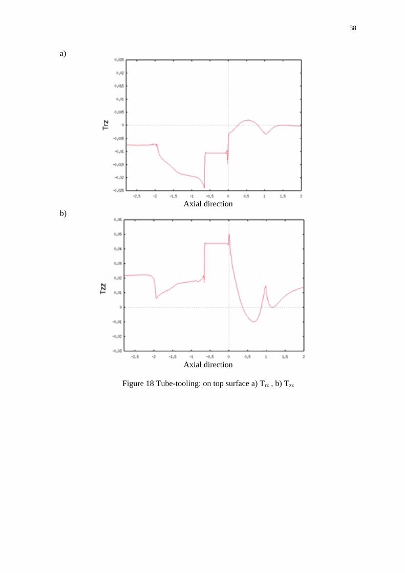
Component stress profiles along the top surface are provided in Figure 18: a) for τrz and b)for τzz. One may observe from this, that along the inlet-tube, τzz is constant, of about 0.02units. Sudden change occurs with each adjustment in geometry. An increase of τzz isobserved within the converging cone of the die, reaching a value of 0.045 units at theentrance to the land-region. τzz is constant over the land-region, followed by a suddenincrease due to singularity, where the polymer departs from the die to the draw-downsection. A sharp decrease within the draw-down is generated. When the polymer makescontact with the wire, τzz increases providing a residual stress of about 0.012 units. Incontrast, the shear-stress τrz is lower in value than the τzz component, as displayed inFigure 18a. τrz starts with a value of about 0.007 units at the inlet tube, increases over theconverging cone to reach a constant value of 0.01 units across the land-region.Subsequently, τrz decreases in the draw-down and coating regions to a minimum valueless than 0.001 units. Contours are plotted in Figure 19 to analyse the state of stress overthe whole domain and in various components. τrr can be considered to be small in theinlet-tube and land-region: it is significant in the converging cone, draw-down and coatingregions. A maximum of about 0.05 units is realised in the draw-down section. For τrz, weobserve a peak (0.024 units) in the converging die-cone, near the entrance to the land-region. The shear-stress is also prominant in the land-region, but of less magnitude (abouthalf) than that over the converging cone. Axial τzz stress is most significant in the land-region, as observed in Figure 19c. The maximum value, 0.051 units, is double that of theshear-stress. Hence, residual stressing to the coating is dominated by the axial component.

15

6.4 Parallel Timings

Parallel computation is employed, within the simulations performed through a spatialdomain decomposition method. The domain of interest is decomposed into a number ofsubdomains, according to available resources and total number of DOF. In this study,uniform load distribution is ensured using a Recursive Spectral Bisection method [34].Though the method is quite general, uniform load may be organized if domain subdivisionis straightforward, otherwise loading will be approximately uniform, from which manualadjustment may be made. As the short-die domain has relatively few DOF, the domain isdecomposed into instances with only two and four sub-domains. In contrast, tube-toolingand pressure-tooling domains are partitioned into as many as eight sub-domains.

In Table 4, information is presented on domain decomposition, the number of elementsand nodes per subdomain, the number of interfacing nodes and ratio of subdomain nodesto interfacing nodes (Cn = Nn:Inn). With an increasing number of subdomains, interfacingnodes (Inn) increase (as does communication cost), whilst the number of elements, nodes(Nn) and degrees-of-freedom per subdomain decreases.

Interface Nodes CnDomain Elements/Subdomain

Nodes/Subdomain

Master Slave Master SlaveShort-Die

1 288 377 - - - -2 144 325 13 13 4% 4%4 72 169 39 26 23% 15.4%

Pressure-Tooling1 3810 7905 - - - -2 1905 3968 31 31 0.78% 0.78%4 953 1976 93 62 4.71% 3.14%8 476 988 217 62 22.0% 6.28%

Tube-Tooling1 4714 9755 - - - -2 2357 4878 31 31 0.64% 0.64%4 1178 2439 103 67 4.22% 2.75%8 589 1222 272 71 22.3% 5.81%

Table 4: Domain Decomposition Data

Parallel timings are generated on a networked cluster of single processor Intel 450 MHzSolaris workstations, a distributed-memory homogeneous platform. A public domainPVM3.4.3 version for message passing protocol has been employed to support inter-processor communication through networking with fast 100 MBit/s EtherNet. Computedresults are presented through the parallel performance of the Taylor-Galerkin scheme, bymeasuring metrics of speed-up and efficiency, with increasing numbers of processors(hence, sub-tasks). The total speed-up (Sn) factor and efficiency (ηn) are defined as:

n

seqn T

TS = ,

n

Snn =η ,

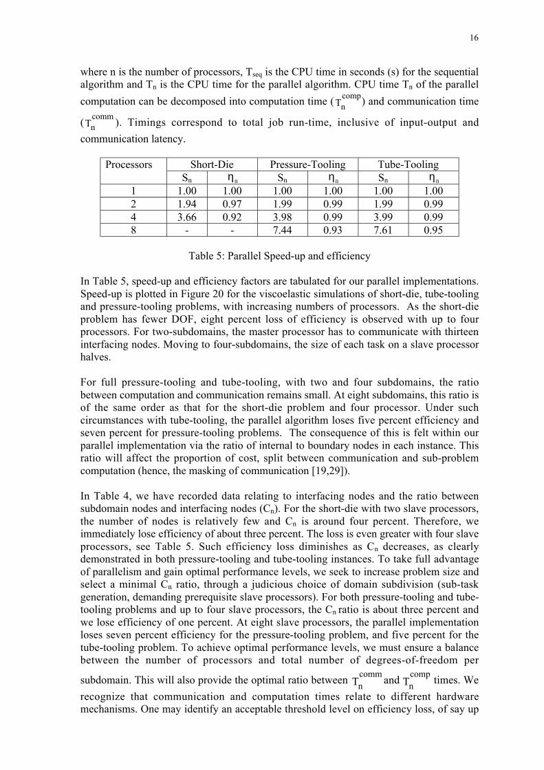
16

where n is the number of processors, Tseq is the CPU time in seconds (s) for the sequentialalgorithm and Tn is the CPU time for the parallel algorithm. CPU time Tn of the parallel

computation can be decomposed into computation time (compnT ) and communication time

(commnT ). Timings correspond to total job run-time, inclusive of input-output and

communication latency.

Short-Die Pressure-Tooling Tube-ToolingProcessorsSn ηn Sn ηn Sn ηn

1 1.00 1.00 1.00 1.00 1.00 1.002 1.94 0.97 1.99 0.99 1.99 0.994 3.66 0.92 3.98 0.99 3.99 0.998 - - 7.44 0.93 7.61 0.95

Table 5: Parallel Speed-up and efficiency

In Table 5, speed-up and efficiency factors are tabulated for our parallel implementations.Speed-up is plotted in Figure 20 for the viscoelastic simulations of short-die, tube-toolingand pressure-tooling problems, with increasing numbers of processors. As the short-dieproblem has fewer DOF, eight percent loss of efficiency is observed with up to fourprocessors. For two-subdomains, the master processor has to communicate with thirteeninterfacing nodes. Moving to four-subdomains, the size of each task on a slave processorhalves.

For full pressure-tooling and tube-tooling, with two and four subdomains, the ratiobetween computation and communication remains small. At eight subdomains, this ratio isof the same order as that for the short-die problem and four processor. Under suchcircumstances with tube-tooling, the parallel algorithm loses five percent efficiency andseven percent for pressure-tooling problems. The consequence of this is felt within ourparallel implementation via the ratio of internal to boundary nodes in each instance. Thisratio will affect the proportion of cost, split between communication and sub-problemcomputation (hence, the masking of communication [19,29]).

In Table 4, we have recorded data relating to interfacing nodes and the ratio betweensubdomain nodes and interfacing nodes (Cn). For the short-die with two slave processors,the number of nodes is relatively few and Cn is around four percent. Therefore, weimmediately lose efficiency of about three percent. The loss is even greater with four slaveprocessors, see Table 5. Such efficiency loss diminishes as Cn decreases, as clearlydemonstrated in both pressure-tooling and tube-tooling instances. To take full advantageof parallelism and gain optimal performance levels, we seek to increase problem size andselect a minimal Cn ratio, through a judicious choice of domain subdivision (sub-taskgeneration, demanding prerequisite slave processors). For both pressure-tooling and tube-tooling problems and up to four slave processors, the Cn ratio is about three percent andwe lose efficiency of one percent. At eight slave processors, the parallel implementationloses seven percent efficiency for the pressure-tooling problem, and five percent for thetube-tooling problem. To achieve optimal performance levels, we must ensure a balancebetween the number of processors and total number of degrees-of-freedom per

subdomain. This will also provide the optimal ratio between commnT and

compnT times. We

recognize that communication and computation times relate to different hardwaremechanisms. One may identify an acceptable threshold level on efficiency loss, of say up

17

to five percent. For the present study, this would imply the efficient use of two slave-processors for the short-die problem, four slave-processors for pressure-tooling and eightslave-processors for tube-tooling. With the proviso of sufficient processors, largerproblems may be tackled in this manner.

7. CONCLUSIONS

In the case of short-die pressure-tooling flow, there was no melt-wire sudden contact andsmooth solutions were established on the wire at the die-exit. For the full-die study incontrast to the short-die, ranges of shear rise ten-fold and extension rate by one hundredtimes. For dimensional equivalents, one must scale by O(103). For the short-die tooling,the major observations are: maximum shear rates arise at die-exit, top-surface, whilst forextension rates they lie within the free-jet region. The corresponding situation for strainrates is more marked, but displaying similar trends to shear rate. Axial stress maximaoccur at the top surface on die-exit. For full-die pressure-tooling, shear rate maxima onthe top surface occur over the land-region, and in particular, peak at the die-exit. The levelis some fifteen times larger than that for the short-die. Shear rate maxima on the wire arelower than that at the top surface, by a factor of three. The double (sudden shock) peaks inshear rate at the bottom surface for full-die flow, do not appear in the short-die case.These are a new feature, introduced as a consequence of the full-die and melt-wirecontact. There is a double peak along the wire, with the die-exit value being marginallylarger than that at melt-wire contact. Extension rate maxima are lower than shear rates byone order, but have increased one hundred fold from the short-die case. Extension ratespeak at the melt-wire contact and across land/die-exit region. The maximum correspondsto the die-exit. The pressure drop across the flow is almost entirely confined to the land-region, and is magnified some twenty-two times over that for the short-die. The behaviourin stress for full-tooling reveals the "shock impact" as the fluid makes contact with thewire. The largest axial stress arises at the melt-wire contact point. The swelling ratios forthe EPTT models are 15% higher than that observed for short-die tooling. Hence, theinfluence of the die flow itself is exposed. The adequacy of the free-surface procedures isalso commended.

In contrast, focusing on tube-tooling design, stress and pressure build-up is realised in theland-region section, as with pressure-tooling. The principal stress component τzz issignificant at the end of the coating, generating a residual stress of about 0.012 units andvanishing shear-stress. This is similar to pressure-tooling. Shear-rates are of O(102) units,reaching a maximum of 144 units, a quarter of that corresponding to the pressure-toolingproblem. This maximum is observed at the exit of the die. Tube-tooling strain-rates are anorder of magnitude lower than tube-tooling shear-rates: strain-rate maxima reach 4.43units, again one quarter of those for pressure-tooling. Largest strain-rates are generatedthroughout the converging die-tube, with lesser values in the draw-down section(extrudate). Such elements of variation between designs would have considerable impactupon the processes involved.

Distributed parallel processing has been shown to be an effective computational tool tosimulate industrial wire-coating flows. Ideal linear speed-up in run-times has beenextracted, based on the number of processors utilised. Increasing the size of the problem,would render even greater efficiency, providing a wider pool of processors were madeavailable.

18

REFERENCES

1. V. Ngamaramvaranggul and M. F. Webster, Simulation of Pressure-Tooling Wire-Coating Flow with Phan-Thien/Tanner Models, Int. J. Num. Meth. Fluids, vol 38,pp 677-710, (2002).

2. T. S. Chung, The Effect of Melt Compressibility on a High-Speed Wire-CoatingProcess, Polym. Eng. Sci., vol 26, no. 6, pp 410-414, (1986).

3. Z. Tadmor, R. B. Bird, Rheological Analysis of Stabilizing Forces in Wire-Coating Die, Polym. Eng. Sci., vol 14, no. 2, pp 124-136, (1974).

4. I. Mutlu and P. Townsend and M. F. Webster, Computation of Viscoelastic CableCoating Flows, Int. J. Num. Meth. Fluids, vol 26, pp 697-712, (1998).

5. B. Caswell and R. I. Tanner, Wire Coating Die Design Using Finite ElementMethods, J. Polym. Sci., vol 18, no. 5, pp 416-421, (1978).

6. J. F. T. Pittman and K. Rashid, Numerical Analysis of High-Speed Wire Coating,Plast. Rub. Proc. Appl., vol 6, p 153, (1986).

7. E. Mitsoulis, Finite Element Analysis of Wire Coating, Polym. Eng. Sci., vol 26,no. 2, pp 171-186, (1986).

8. E. Mitsoulis and R. Wagner and F. L. Heng, Numerical Simulation of Wire-Coating Low-Density Polyethylene: Theory and Experiments, Polym. Eng. Sci.,vol 28, no. 5, pp 291-310, (1988).

9. R. Wagner and E. Mitsoulis, Adv. Polym. Tech., vol 5, p 305 (1985).

10. H. Matallah and P. Townsend and M. F. Webster, Viscoelastic Computations ofPolymeric Wire-Coating Flows, Int. J. Num. Meth. Heat Fluid Flow, accepted forpublication 2001, available as CSR 13-2000, University of Wales, Swansea.

11. C. D. Han and D. Rao, Studies on Wire Coating Extrusion. I. The Rheology ofWire Coating Extrusion, Polym. Eng. Sci., vol 18, no.13, pp 1019-1029, (1978).

12. K. U. Haas and F. H. Skewis, SPE ANTEC Tech. Paper, vol 20, p 8, (1974).

13. D. M. Binding and A. R. Blythe and S. Gunter and A. A. Mosquera and P.Townsend and M. F. Webster, Modelling Polymer Melt Flows in Wire CoatingProcesses, J. Non-Newtonian Fluid Mech., vol 64, pp 191-209, (1996).

14. I. Mutlu and P. Townsend and M. F. Webster, Simulation of Cable-CoatingViscoelastic Flows with Coupled and Decoupled Schemes, J. Non-NewtonianFluid Mech., vol 74, pp 1-23, (1998).

15. H. Matallah and P. Townsend and M. F. Webster, Viscoelastic Multi-ModeSimulations of Wire-Coating, J. Non-Newtonian Fluid Mech., vol 90, pp 217-241,(2000).

16. V. Ngamaramvaranggul and M.F. Webster, Simulation of Coatings Flows withSlip Effects; Int. J. Num. Meth. Fluids, vol 33, pp 961-992, (2000).

17. V. Ngamaramvaranggul and M. F. Webster, Computation of Free Surface Flowswith a Taylor-Galerkin/Pressure-Correction Algorithm, Int. J. Num. Meth. Fluids,vol 33, pp 993-1026, (2000).

18. V. Ngamaramvaranggul and M. F. Webster, Viscoelastic Simulations of Stick-Slipand Die-Swell Flows, Int. J. Num. Meth. Fluids, vol 36, pp 539-595, (2001).

19

19. A. Baloch, P. W. Grant, M. F. Webster, Homogeneous and heterogeneousdistributed cluster processing for two and three-dimensional viscoelastic flows,submitted to Int. J. Num. Meth. Fluids, available as CSR 16-2000.

20. N. Phan-Thien and R. I. Tanner, A New Constitutive Equation Derived fromNetwork Theory, J. Non-Newtonian Fluid Mech., vol 2, pp 353-365, (1977).

21. N. Phan-Thien, A Non-linear Network Viscoelastic Model, J. Rheol., vol 22, pp259-283, (1978).

22. N. Phan-Thien and R. I. Tanner, Boundary-Element Analysis of FormingProcesses in 'Numerical Modelling of Material Deformation Processes: Research,Development and Application’ by P. Hartley, I. Pillinger and C. Sturgess (Eds)Springer-Verlag, London, (1992).

23. P. Townsend, M.F. Webster, An algorithm for the three-dimensional transientsimulation of non-Newtonian fluid flows, in G. Pande, J. Middleton (Eds.), Proc.Int. Conf. Num. Meth. Eng.: Theory and Applications, NUMETA, Nijhoff,Dordrecht, pp.T12/1-11, (1987).

24. D. M. Hawken, H. R. Tamaddon-Jahromi, P. Townsend, M. F. Webster, A Taylor-Galerkin-based algorithm for viscous incompressible flow, Int. J. Num. Meth.Fluid, vol 10, pp 327-351, (1990).

25. E. O. A. Carew and P. Townsend and M. F. Webster, A Taylor-Petrov-GalerkinAlgorithm for Viscoelastic Flow, J. Non-Newtonian Fluid Mech., vol 50 , pp253-287, (1993).

26. A. Baloch, M. F. Webster, A computer simulation of complex flows of fibresuspensions, Computers Fluids vol 24 (2), pp 135-151, (1995).

27. A. Baloch, P. Townsend, M. F. Webster, On the highly elastic flows, J. Non-Newtonian Fluid Mech. vol 75, pp 139-166, (1998).

28. H. Matallah, P. Townsend, M. F. Webster, Recovery and stress-splitting schemesfor viscoelastic flows, J. Non-Newtonian Fluid Mech. vol 75, pp 139-166, (1998).

29. P.W. Grant, M.F. Webster and X. Zhang, Coarse Grain Parallel Simulation forIncompressible Flows, Int. J. Num. Meth. Eng., vol 41, pp 1321-37, (1998).

30. S. Richardson, A “stick-slip” problem relatived to the motion of a free jet at lowReynolds numbers, Proc. Camb. Phil. Soc., vol 67, pp 477-489, (1970).

31. M. J. Crochet, A. R. Davies and K. Walter, Numerical Simulation of Non-Newtonian Flow, Rheology Series 1, Elsevier Science Publishers, (1984).

32. R. I. Tanner, Engineering Rheology, Oxford University Press, London, (1985).

33. V. Ngamaramvaranggul, Numerical Simulation of Non-Newtonian Free SurfaceFlows, PhD thesis, University of Wales, Swansea (2000).

34. H.D. Simon, Partitioning of unstructured problems for parallel processing,Computer Systems in Engineering, vol 2, pp 135-148, (1991).

20

FIGURE LEGEND

Table 1: Finite element mesh dataTable 2: a) Full-die pressure-tooling; mesh characteristics, sub-region zones

b) Tube-tooling; mesh characteristics, sub-region zonesTable 3: Short-die and full-die; EPTT(1,0,0.99), We=200, solution valuesTable 4: Domain decomposition dataTable 5: Parallel speed-up and efficiency

Figure 1: EPTT model: (a) shear viscosity; (b) elongational viscosityFigure 2: Short-die pressure-tooling:(a) schema, (b) mesh, 6x24 elementsFigure 3: Full-die pressure-tooling:(a) schema, (b) mesh, 15x127 elementsFigure 4: Full-die tube-tooling:(a) schema, (b) mesh, 4714 elementsFigure 5: Short-die: (a) pressure contours, (b) I2 contours, (c) ε̇ contoursFigure 6: Short-die: (a) pressure along the wire, (b) I2 on top surface,

(c) die swell on top freeFigure 7: Short-die: (a) Trr contours, (b) Trz contours, (c) Tzz contoursFigure 8: Short-die: Trz (a) on top surface, (b) on wireFigure 9: Short-die: Tzz a) on top surface, (b) on wireFigure 10: Full-die pressure-tooling: (a) pressure contours, (b) I2 contours, (c) ε̇ contoursFigure 11: Full-die pressure-tooling: (a) pressure along the wire, (b) die swell on top freeFigure 12: Full-die pressure-tooling: I2 (a) on top surface, (b) on bottom surfaceFigure 13: Full-die pressure-tooling: (a) Trr contours, (b) Trz contours, (c) Tzz contoursFigure 14: Full-die pressure-tooling: Trz (a) on top surface, (b) on wireFigure 15: Full-die pressure-tooling: Tzz a) on top surface, (b) on wireFigure 16: Tube-tooling: (a) pressure contours, (b) I2 contours, (c) ε̇ contoursFigure 17: Tube-tooling: (a) pressure along the wire, (b) I2 on top surface,

(c) I2 on bottom surfaceFigure 18: Tube-tooling: on top surface (a) Trz (b) Tzz

Figure 19: Tube-tooling: (a) Trr contours, (b) Trz contours, (c) Tzz contours

Figure 20: Parallel speed-up

21

(a) Shear viscosity

(b) Extensional viscosityFigure 1. EPTT(1, 0.99, 200)

22

Figure 2. Die swell/drag flow: a) schema

Figure 2. Die swell/drag flow: b) mesh pattern, 6x24 elements

23

Figure 3a. Pressure-tooling: schema

Figure 3b. Pressure-tooling: mesh pattern, 15x127 elements

24

Figure 4a. Tube-tooling: schema

Figure 4b. Tube-tooling: mesh pattern, 4714 elements

25

a)

b)

c)

Figure 5: Short-die: (a) pressure contours, (b) I2 contours, (c) ε̇ contours

26

a)

b)

c)

Figure 6: Short-die: (a) pressure along the wire, (b) I2 on top surface,(c) die swell on top free

27

a)

b)

c)

Figure 7: Short-die: (a) Trr contours, (b) Trz contours, (c) Tzz contours

28

a)

b)

Figure 8: Short-die: Trz (a) on top surface, (b) on wire

29

a)

b)

Figure 9: Short-die: Tzz a) on top surface, (b) on wire

30

a)

b)

c)

Figure 10: Full-die pressure-tooling: (a) pressure contours, (b) I2 contours, (c) ε̇ contours

31

a)

b)

Figure 11: Full-die pressure-tooling: (a) pressure along the wire, (b) die swell on top free

32

a)

b)

Figure 12: Full-die pressure-tooling: I2 (a) on top surface, (b) on bottom surface

33

a)

b)

c)

Figure 13: Full-die pressure-tooling: (a) Trr contours, (b) Trz contours, (c) Tzz contours

34

a)

b)

Figure 14: Full-die pressure-tooling: Trz a) on top surface, (b) on wire

35

a)

b)

Figure 15: Full-die pressure-tooling: Tzz a) on top surface, (b) on wire

36

a)

b)

c)

Figure 16 Tube-tooling: a) pressure contours, b) I2 contours, c) ε̇ contours

37

a)

Axial directionb)

Axial directionc)

Axial directionFigure 17 Tube-tooling: a) pressure along the wire; b) I2 on top surface; c) I2 on wire

38

a)

Axial directionb)

Axial direction

Figure 18 Tube-tooling: on top surface a) Trz , b) Tzz

39

a)

b)

c)

Figure 19 Tube-tooling: a) Trr contours, b) Trz contours, c) Tzz contours

40

Figure 20: Parallel speed-up