simulation of nanoparticles formation by mechanism of...

Res

earc

h A

rtic

le: O

pen

Acc

ess

International Journal of

Nanoparticles and Nanotechnology

Received: August 22, 2017: Accepted: December 09, 2017: Published: December 11, 2017

Citation: Sarychev V, Nevskii S, Alexey G, Chinakhov D (2017) Simulation of Nanoparticles Formation by Mechanism of Kelvin-Helmholtz Instability. Int J Nanoparticles Nanotech 3:012

Copyright: © 2017 Sarychev V, et al. This is an open-access article distributed under the terms of the Creative Commons Attribution License, which permits unrestricted use, distribution, and reproduction in any medium, provided the original author and source are credited.

*Corresponding author: Sergey Nevskii, Siberian State Industrial University, 654007, Novokuznetsk, Russia, E-mail: [email protected]

Sarychev et al. Int J Nanoparticles Nanotech 2017, 3:012

Simulation of Nanoparticles Formation by Mechanism of Kelvin-Helmholtz InstabilityVladimir Sarychev1, Sergey Nevskii1*, Granovskii Alexey1 and Dmitriy Chinakhov2

1Siberian State Industrial University, Novokuznetsk, Russia2Yurga Institute of Technology, Tomsk Polytechnic University, Yurga, Russia

IntroductionHydrodynamic concept to determine the mechanism

for forming nanostructured elements under external ac-tions was first used when studying effects of heteroge-neous plasma flows, created by electric explosion of con-ductors, on metals [1]. This work introduces a hypothe-sis that nanostructures in a metal are formed because of the Kelvin-Helmholtz instability. An ideal fluid models a layer of plasma and a viscous fluid models a molten layer. Using the Navier-Stokes equations for linear analysis in hydrodynamics relating to small perturbations allowed us to obtain a dispersion equation, with its numerical

AbstractThe Kelvin-Helmholtz instability is analyzed at scales of micro-and nano-structures. We have studied the stability of a plane motionless layer of a two-layer incompressible viscous fluid using the Navier-Stokes equations for linear and nonlinear analyses. The effects of viscosity were assumed to occur at an interface with a flow inside the layers to be irrotational. A dispersion equation was developed for small perturbations, which is similar in form to the dispersion equation appeared in earlier papers, provided the short-wave approximation is applied. We first determined: 1) The dependence of the perturbation decrement for a viscous two-layer fluid that has two maxima, with the first maximum being within the wavelengths ranging from 100 to 300 nm and the second from 1 to 3 μm; 2) The approximate analytic dependence of wavenumber that contains the maximum for the perturbation decrement on input parameters for a problem (densities of both layers, their thicknesses, viscosity, surface tension, velocity of layer motion, a coefficient of resistance). It allows us to size up the emerging vortex structures under different conditions. The range of input parameters for the problem was determined, where two maxima relating to the dependence of disturbance decrement were observed. To verify the results after performing linear analysis, the Level Set Method was used for analyzing nonlinear equations. The results of calculations prove that linear analysis adequately describes how vortex structures in various sizes are formed.

KeywordsKelvin-Helmholtz instability, Navier-Stokes equations, Level set method

solution making possible to obtain the dependence of increment on wavelength. The maximum in this depen-dence is achieved at a wavelength λm. With certain values of parameters for the problem (density, layer thickness, viscosity, tension coefficients and relative velocity), the wavelength λm is in the nanometer range. This means that the waves within this wavelength region will prog-ress, and after the molten layer solidifies these waves can be observed using an electron microscope. Photographs representing the characters of metal surfaces are given in [1]. Thus, it can be said that the proposed model for forming nanostructures allows us to obtain, in principle,

• of 10 •



the dependence of critical wavelength on the parameters. However, the dispersion equation is complicated by al-lowing for viscosity, even while considering one layer and, therefore, the parameterization can be carried out only in terms of numbers in the case of semi-infinite layers. The finiteness of layers taken into account leads to a more complicated dispersion equation [2]. Under the assumption of a viscous potential flow, a simplified dispersion equation was obtained in [3], but its para-metric analysis in these and subsequent works of these authors was not carried out. The work in [2] gives a nu-merical analysis of the complete equation and an ana-lytic-graphical analysis of the dispersion equation under the assumption of the viscous potential flow. The depen-dence of the increment on the wavelength having two maxima was found for certain parameters. This suggests that even in the first linear approximation there can ex-ist two scales. With a purpose of obtaining a simplified dispersion equation, the case of short waves was consid-ered in [4,5]. In this approximation, the dispersion equa-tion was derived that coincides with the equation for the visco-potential model [3]. It is shown that from the ob-tained equation it is possible to explicit the increment as a function of wavenumber and parameters that facilitates to find the conditions required for forming two maxima, and to give approximate expressions for the two values of λm. In our opinion, this allows us to carry out parameter-ization in various physical conditions with the purpose of identifying conditions for the formation of nanostruc-tures. Therefore, an important role in our study plays a visco-potential flow.

The fluid mechanics theory of potential flow goes back to Euler in 1761. The concept of viscosity was not known in Euler’s time. The effects of viscous stresses were introduced by Navier (1822) and Stokes (1845). Stokes (1851) considered potential flow of a viscous fluid in an approximate sense, but later authors restrict their attention to “potential flow of an inviscid fluid”. All the books on fluid mechanics and all courses in fluid me-chanics have chapters on “potential flow of inviscid flu-ids” and none on the “potential flow of a viscous fluid” or “Viscous Potential Flow” (VPF). An authoritative and readable exposition of irrotational flow theory and its applications can be found in chapter 6 of the book on fluid dynamics [6]. He speaks of the role of the theory of flow of an inviscid fluid: “various aspects of the flow of a fluid regarded as entirely inviscid (and incompressible) will be considered. The results presented are significant only in as much as they represent an approximation to the flow of a real fluid at large Reynolds number and the limitations of each result must be regarded as important as the result itself”. In book [7] has considered irrota-tional flows of a viscous fluid. That is of the opinion that when one is considering irrotational solutions of the Na-

vier-Stokes equations it is never necessary and typically not useful for one to put the viscosity to zero. This obser-vation runs counter to the idea frequently expressed that potential flow is a topic that is useful only for inviscid fluids; many people think that the notion of a viscous potential flow is an oxymoron. Incorrect statements like “irrotational flow implies inviscid flow but not the other way around” can be found in popular textbooks. The [3] argues that the Navier-Stokes equations are satisfied by potential flow; the viscous term is identically zero when the vorticity is zero but the viscous stresses are not zero. It is not possible to satisfy the no-slip condition at a sol-id boundary or the continuity of the tangential compo-nent of velocity and shear stress at a fluid-fluid boundary when the velocity is given by a potential. KH instability is included by a discontinuity of the velocity at a two-fluid interface. This discontinuity is inconsistent with the no-slip condition for Navier-Stokes studies of viscous fluids, but is consistent with the theory of potential flow of a viscous fluid. Viscous potential flow analysis gives good approximations to fully viscous flows in cases where the shears from the gas flow are negligible. In addition, in [4], it is shown that in the case of short waves the dis-persion equation for the viscous layer coincides with the dispersion equation of the VPF. Then analysis is based on the viscous potential flow theory in this paper.

We can observe nanostructured elements in materi-als not only under the influence of concentrated energy flows, but also intense plastic deformation. An example is equal-channel angular pressing [8], shift under pres-sure [9], friction and wear processes [10,11] and long-term service life of rails [12,13]. We pay special atten-tion to the papers in [10,11]. In these works, the shear instability of subsurface layers in friction was studied. With the help of scanning electron microscopy [10] it was established that, as moving from the depth of met-al to the surface of friction, several characteristic zones can be distinguished: The zone of plastic deformation and texturing (I), the zone of intense fragmentation (II), the zone of turbulent flow (III), and the zone of laminar flotation (VI). The authors [10] designate Zones I and II as the zones of ordinary plastic deformation, whereas Zones III and IV, in their opinion, relate to the zones of shear instability similar to the Kelvin-Helmholtz insta-bility at the shear boundary. To evaluate the availability of such a phenomenon, the authors [10] used the ap-proach proposed yet by Heisenberg [14] and Lin [15]. The use of these results in works [10] and [11] helps to conclude that the pattern of plastic flow is similar to the flow of a fluid. The work [11] describes a material with the layer of a nanoscale grain structure, produced by the experimental process. However, these articles only men-tion the Kelvin-Helmholtz instability, but its analytical results are not used.

• of 10 •



This paper is structured as follows: Section 2 sets up the problem. In Section 3 there is a linear analysis of equations of motion with regard to cases relating to vis-cous and viscoelastic fluids, as well as at the interface with a porous medium. Section 4 gives the results after solving nonlinear equations using numerical analysis and their comparison with the results obtained by linear analysis.

Problem FormulationLet us consider the stability of a plane motionless

layer of a two-layer incompressible fluid (Figure 1). We choose the direction of the x-axis along the inter-face between the layers, and the y-axis is perpendicu-lar to x and directed toward the second layer. The first layer ( , ( , ))x h y x tη−∞ < < ∞ − < < is a viscous, visco-elastic or porous motionless medium. The second layer ( , ( , ) )x x t y Hη−∞ < < ∞ < < moves with a velocity u0.

The equation of motion for every layer is expressed as:

,

,

= ik nnn

k n

dudt x

σρ

∂∂

(1)

Where σik is the stress components, n = 1,2 is a num-ber of layers. Kinematic and dynamic boundary condi-tions are explicated as:

2

1

2 2 1 1

1 2

= : v = 0; = : v = 0;

= 0 : = v , = v

0n n

y Hy h

y u ut x t xη η η η

σ σ σ

−∂ ∂ ∂ ∂

+ +∂ ∂ ∂ ∂

− − Κ =

(2)

Where ( )32

= 1 ( )

xx

x

K η

η+ is the surface curva-

ture. The condition for shear stresses is not stated. These

There is no single viewpoint on the applicability of the hydrodynamic approach to the formation of nanostruc-tures in a deformed solid because there are no direct ob-servations of the hydrodynamic instability of the material at this level. Electron microscopy enables the scanning of nanoscale structural elements that have already formed in a liquid metal near the shearing boundary of tangential ve-locity. Note that this method helps to establish that electron diffraction patterns for the nanostructures are of a qua-si-ring structure [16-18] specific to liquid and quasi-liquid media that allows us to conclude that the hydrodynamic vision is applicable. The possibility of using the hydrody-namic approach to describe the intense plastic deformation is also implied by the phenomenon of deformation-induced amorphization investigated in [17,18]. The linear analysis of the Kelvin-Helmholtz instability developed in our works [1-3] to various technological problems is presented in [19]. A mechanism and a mathematical model for the formation of shear bands from the position of the Kelvin-Helmholtz instability are proposed in [20]. Within the framework of this model, a neutral curve is obtained, which allows us to determine only the conditions for the onset of instability. Dependence of the decrement on the wave number was not given. Therefore, it is impossible to determine on what scale the development of instability will occur. In addition, the developed approach allows us to propose technologies for the formation of nanostructured states, for example, nan-odroplets produced with employing plasma-arc processes [21]. In this case, λm corresponds to the size of the nano-drops.

Therefore, our work is aimed at developing a mathemat-ical model that enables parameterization in an approximate model for linear analysis of the Kelvin-Helmholtz instabili-ty, and carry out numerical calculations of nonlinear equa-tions in the context of dependences of wavenumbers on pa-rameters derived at maximum decrement values and on the basis of the identified parameters.

x

y

h−

1

2

,

sPVU ,,,,, 11111 νρ

22222 ,,,, νρ PVU 0u

H

( )x tη

Figure 1: Problem formulation of linear analysis.

• of 10 •



stresses can be calculated if necessary. For an isotropic viscous fluid, the components of stress tensor have the form:

= 2ik ik ikpσ δ µε− + (3)

Where 1 = 2

i kik

k i

u ux x

ε ∂ ∂

+ ∂ ∂ is the rate of strain

tensor, p is the pressure, μ is the fluid viscosity. For cases when the medium is viscoelastic, the stress tensor has the form:

= 2 2ik ik ik ik ikp Gσ δ µε λθδ ε− + + + (4)

Where λ and G are constant, θ is the volumetric strain.

According to the results [5] obtained in an approxi-mation of short waves, the viscosity has an effect occur-ring only at the interface between the layers. Therefore, the Navier-Stokes equations can be replaced with the Euler equations, with the flow in the layers assumed to be free of vortex. Such flows are called viscous-potential. The analysis [5] proves that in this approximation the dispersion equation for waves at the interface of a viscous and an ideal fluid agrees with the dispersion equation in a viscous-potential approximation. Therefore, we intend apply a visco-potential model to viscous, viscoelastic and porous media. According to this model, one can formu-late an expression for pressure. To write the equations to describe the viscous-potential model, we introduce the potential of velocity:

= n nu ∇Φ

(5)

So that the normal components of tensor (3) take the form:

= 2 nn n n

vpy

σ µ ∂− +

∂ (6)

For pressure in viscosity potential flow conditions:

21 = ( )2

nn n np C t

tρ ∂Φ − + ∇Φ + ∂

. The proof of this for-

mula is similar to the conclusion of the Cauchy-Lagrange and for the stationary case, the Bernoulli integral. Arbi-trary function C(t) can be included in Φ.

Linear analysis of the equations of motionWe first consider the two viscous fluids. In this case, it

is necessary to put (3) in (1) and the dynamic boundary condition (2), then after their modification the equations of motion will have the form:

2 2

2 2

2 2

2 2

1 = ,

1 = , = 0

n n n n n nn n n

n

n n n n n n n nn n n

n

u u u p u uu vt x y x x y

v v v p v v u vu vt x y y x y x y

νρ

νρ

∂ ∂ ∂ ∂ ∂ ∂+ + − + + ∂ ∂ ∂ ∂ ∂ ∂

∂ ∂ ∂ ∂ ∂ ∂ ∂ ∂+ + − + + + ∂ ∂ ∂ ∂ ∂ ∂ ∂ ∂

(7)

Where νn is the kinematic viscosity of the n-th layer. We linearize (7) and the boundary conditions (2) relating to small perturbations. In the result, we get the following:

2 2 2 21 1 1 1 1 1 1 1 1 1

1 12 2 2 21 1

1 1 = , = , = 0U P U U V P V V U Vt x x y t y x y x y

ν νρ ρ

∂ ∂ ∂ ∂ ∂ ∂ ∂ ∂ ∂ ∂− + + − + + + ∂ ∂ ∂ ∂ ∂ ∂ ∂ ∂ ∂ ∂

2 22 2 2 2 2

0 2 2 22

2 22 2 2 2 2 2 2

0 2 2 22

1 = ,

1 = , = 0

U U P U Uut x x x y

V V P V V U Vut x y x y x y

νρ

νρ

∂ ∂ ∂ ∂ ∂+ − + + ∂ ∂ ∂ ∂ ∂

∂ ∂ ∂ ∂ ∂ ∂ ∂+ − + + + ∂ ∂ ∂ ∂ ∂ ∂ ∂

(8)

The boundary conditions (2) take the following form:

2

1

0 2 1

1 21 1 2 2

= : = 0; = : = 0

= 0 : = , = ;

2 2 = xx

y H Vy h V

y u V Vt x t

V VP Py y

η η η

µ µ ση

−∂ ∂ ∂

+∂ ∂ ∂

∂ ∂− + + −

∂ ∂

(9)

As mentioned above, we use the model of a vis-cous-potential fluid. To this end, we linearize equation (5). As a result, we get:

1 1 2 21 2 2 = , = ; = , = U V U V

x y x y∂Φ ∂Φ ∂Φ ∂Φ∂ ∂ ∂ ∂

(10)

After that, the continuity equations give the follow-ing:

2 2 2 21 1 2 2

2 2 2 2 = 0, = 0x y x y

∂ Φ ∂ Φ ∂ Φ ∂ Φ+ +

∂ ∂ ∂ ∂ (11)

From the momentum conservation equation, it fol-lows

1 2 21 1 2 2 0 = ; = P P u

t t xρ ρ∂Φ ∂Φ ∂Φ − − + ∂ ∂ ∂

(12)

Allowing for (10) and (12), the boundary conditions (9) are written as

2 1 = : = 0, = : = 0y H y hy y

∂Φ ∂Φ−

∂ ∂

2 10 = 0 : = , = y u

t x y t yη η η∂Φ ∂Φ∂ ∂ ∂

+∂ ∂ ∂ ∂ ∂

(13)

2 2 21 1 2 2 2

1 1 1 2 0 2 22 2 22 2 = ut y t x y x

ηρ ρν ρ ρ ν σ∂Φ ∂ Φ ∂Φ ∂Φ ∂ Φ ∂ + − + − ∂ ∂ ∂ ∂ ∂ ∂

Thus, the formulated mathematical problem reduces to solving the Laplace’s equations (12) with the boundary conditions (13). The solution to the Laplace’s equations satisfying (13) can be written in the form:

1 1 2 2 = exp( )cosh( ( )), = exp( )cosh( ( )), = exp( ), = 2

A t ikx k y h A t ikx k y HB t ikx k

ω ωη ω π λΦ − + Φ − −

− (14)

Substitution of (14) into Equations (11) and (13) gives a system of algebraic equations for A1, A2, B. If this de-terminant set to zero, we obtain the dispersion equation:

( ) ( )2 2 3 2 2 31 2 2 0 1 1 2 2 0 2 2 2 02 (2 2 ) (2 )R R iR u k R R k u iR k R k u kω ω ν ν ν σ+ + + + − − + (15)

Where 1 1 = coth( ),R khρ 2 2 = coth( ).R kHρ We rewrite this equation in the form:

212 ( ) = 0a ib c icω ω+ + + + (16)

• of 10 •



( )21 2

1 = ( ) ,1

a A kA

ν ν++

0 = ,1Akub

A+ 2 2 20 0 = ,

1k u Ac

Aω −

+ 3

2 01

2 = 1

k u AcA

ν+

Where 2 1 = / .A R R We note that the dispersion equa-tion (16) follows the dispersion equation derived in [4] with the use of the short-wave approximation. Thus, we assume the flow of material is irrotational in the layers and the effect of viscosity at the interface is significant and these assumptions make possible to obtain the dis-persion equation for short waves without additional conditions. From (16), by substituting = ,iω α + Ω with subsequent modification, we express the dependence of decrement α on wavenumber k:

2 2 2 214 ( 1)

= 2a b

aδ δ δ

α + + − −

(17)

Where 2 2 11 = , = .

2ca b cab

δ δ− − We now search for val-

ues of wavenumber at which (18) takes on the maximum value. If α > 0, then is instability regions, and contra: if α < 0, then stability. Achieving the maximum value by α = α(k) dependence means that the waves with a wave-number of ~kmax will progress. These waves will generate particles with dimensions ~λmax [22]. Equation (17) is suitable for numerical analysis. However, obtaining the dependence of wavelength that includes the maximum α(k) on the problem parameters suggests a cluttered ap-pearance in equations, the physical meaning of which is difficult to comprehend. Therefore, it is necessary to solve the problem of finding an approximate analytical dependence λmax on the problem parameters. To this end, we transform (17) to the following form:

2 214

= 12

f f faα

+ + −

(18)

Where 2 2

112 2

/ 2 = , = ab ca b cf fa a

−− − . Thus, the behavior of decrement with regard to wavenumber depends on the be-havior of functions f and f1. Let us consider two cases. The first case is 12 ff > . In this case, (18) will have the form:

( )

( )1

21

1, 0;1 21 =

2 / 1, 0.

= /

f ff fa a

f f f

f f

εα

ε

− >+ + ≈ − − − < (19)

The second case is 12 ff < :

( ) ( )2

1 1 21

1

2 1 ( / 2 ) / 21 = / 2 1 1 ,

2

= / 2

f f f fa a f z z

z f f

α + + ≈ − + + −

(20)

The substitution of f and f1 in (19) and subsequent transformations result in

2 21 0 1 2

1

20 1 2

2 1 220

1

1 = ( (1 ) ) ( )1

( ) = ( )1

(1 )

kk A Au A kA R

Auk AA k A Au

R

σα ν ν

ν να ν νσ

− + − − + +

− − + ++ −

(21)

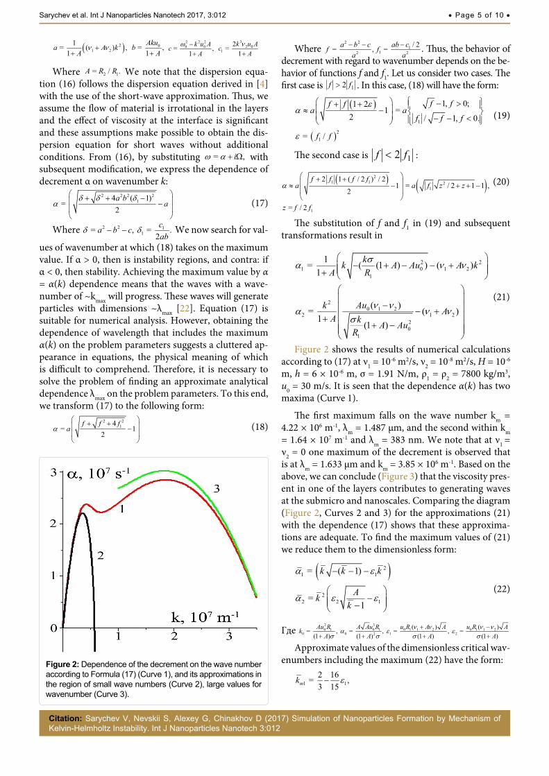
Figure 2 shows the results of numerical calculations according to (17) at ν1 = 10-6 m2/s, ν2 = 10-8 m2/s, H = 10-6 m, h = 6 × 10-6 m, σ = 1.91 N/m, ρ1 = ρ2 = 7800 kg/m3, u0 = 30 m/s. It is seen that the dependence α(k) has two maxima (Curve 1).

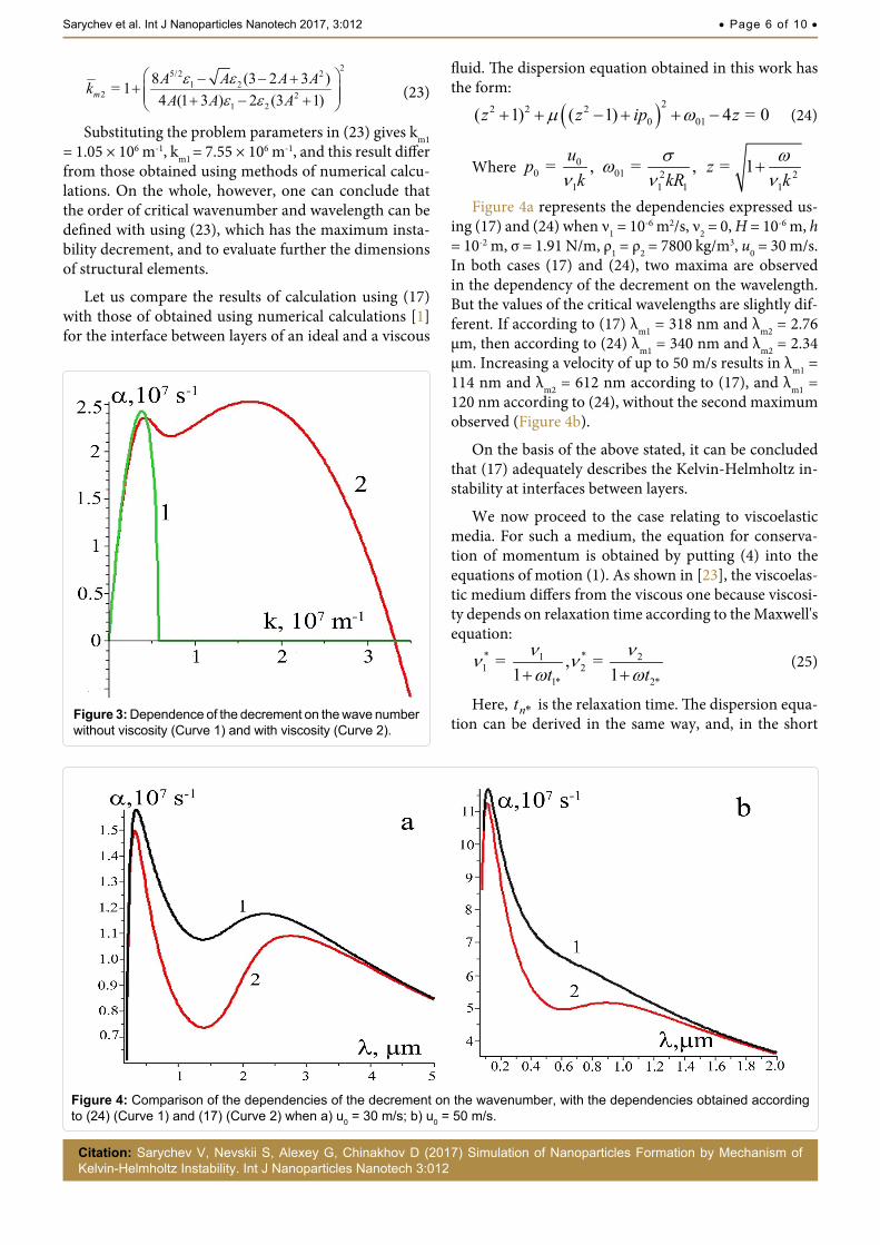
The first maximum falls on the wave number km = 4.22 × 106 m-1, λm = 1.487 μm, and the second within km = 1.64 × 107 m-1 and λm = 383 nm. We note that at ν1 = ν2 = 0 one maximum of the decrement is observed that is at λm = 1.633 μm and km = 3.85 × 106 m-1. Based on the above, we can conclude (Figure 3) that the viscosity pres-ent in one of the layers contributes to generating waves at the submicro and nanoscales. Comparing the diagram (Figure 2, Curves 2 and 3) for the approximations (21) with the dependence (17) shows that these approxima-tions are adequate. To find the maximum values of (21) we reduce them to the dimensionless form:

( )21 1

22 2 1

= ( 1)

= 1

k k k

Akk

α ε

α ε ε

− − −

− −

(22)

Где 2 30 1 0 1 0 1 1 2 0 1 1 2

0 0 1 22

( ) ( ) = , = , = , = (1 ) (1 ) (1 ) (1 )Au R A Au R u R A A u R Ak

A A A Aν ν ν να ε ε

σ σ σ σ+ −

+ + + +

Approximate values of the dimensionless critical wav-enumbers including the maximum (22) have the form:

1 12 16 = ,3 15mk ε−

Figure 2: Dependence of the decrement on the wave number according to Formula (17) (Curve 1), and its approximations in the region of small wave numbers (Curve 2), large values for wavenumber (Curve 3).

• of 10 •



fluid. The dispersion equation obtained in this work has the form:

( )22 2 20 01( 1) ( 1) 4 = 0z z ip zµ ω+ + − + + − (24)

Where 00

1

= ,upkν

01 21 1

= ,kRσω

ν 2

1

= 1zk

ων

+

Figure 4а represents the dependencies expressed us-ing (17) and (24) when ν1 = 10-6 m2/s, ν2 = 0, H = 10-6 m, h = 10-2 m, σ = 1.91 N/m, ρ1 = ρ2 = 7800 kg/m3, u0 = 30 m/s. In both cases (17) and (24), two maxima are observed in the dependency of the decrement on the wavelength. But the values of the critical wavelengths are slightly dif-ferent. If according to (17) λm1 = 318 nm and λm2 = 2.76 µm, then according to (24) λm1 = 340 nm and λm2 = 2.34 µm. Increasing a velocity of up to 50 m/s results in λm1 = 114 nm and λm2 = 612 nm according to (17), and λm1 = 120 nm according to (24), without the second maximum observed (Figure 4b).

On the basis of the above stated, it can be concluded that (17) adequately describes the Kelvin-Helmholtz in-stability at interfaces between layers.

We now proceed to the case relating to viscoelastic media. For such a medium, the equation for conserva-tion of momentum is obtained by putting (4) into the equations of motion (1). As shown in [23], the viscoelas-tic medium differs from the viscous one because viscosi-ty depends on relaxation time according to the Maxwell's equation:

* *1 21 2

1* 2*

= , = 1 1t t

ν νν νω ω+ +

(25)

Here, *nt is the relaxation time. The dispersion equa-tion can be derived in the same way, and, in the short

25/2 21 2

2 21 2

8 (3 2 3 ) = 14 (1 3 ) 2 (3 1)mA A A AkA A A

ε εε ε

− − ++ + − +

(23)

Substituting the problem parameters in (23) gives km1 = 1.05 × 106 m-1, km1 = 7.55 × 106 m-1, and this result differ from those obtained using methods of numerical calcu-lations. On the whole, however, one can conclude that the order of critical wavenumber and wavelength can be defined with using (23), which has the maximum insta-bility decrement, and to evaluate further the dimensions of structural elements.

Let us compare the results of calculation using (17) with those of obtained using numerical calculations [1] for the interface between layers of an ideal and a viscous

Figure 3: Dependence of the decrement on the wave number without viscosity (Curve 1) and with viscosity (Curve 2).

Figure 4: Comparison of the dependencies of the decrement on the wavenumber, with the dependencies obtained according to (24) (Curve 1) and (17) (Curve 2) when a) u0 = 30 m/s; b) u0 = 50 m/s.

• of 10 •



Nonlinear numerical analysisWe use the finite element method as a base for nu-

merical analysis to solve nonlinear equations. In recent times, the Level-Set Method (LSM) has been used to solve the hydrodynamic equations of multilayer immis-cible fluids [24]. This method is based on the idea that the motion of interfaces is described by means of the so-called level-set functions that determine a distance from a given point to an interface. The function is assumed to take positive values for points inside the fluid and nega-tive values for points in the empty space. Due to a smooth change in this function when crossing the interface, the effect of diffusion is insignificant at the interface, but for large times the values of the function already cease to have their meaning as distances to the interface, and from time to time the distance to the interface must be redefined in the calculation [25-27]. In this article, calcu-lations are made in the COMSOL Multiphysics package under the following initial conditions:

1 1 2 0 22(0) = 0, (0) = 0, (0) = , (0) = sinm

xu v u u v A πλ

(28)

Where Am is the amplitude of perturbation on the velocity. Figure 5 and Table 1 shows the boundary con-ditions. Table 2 shows the materials characteristics and input parameters of problem.

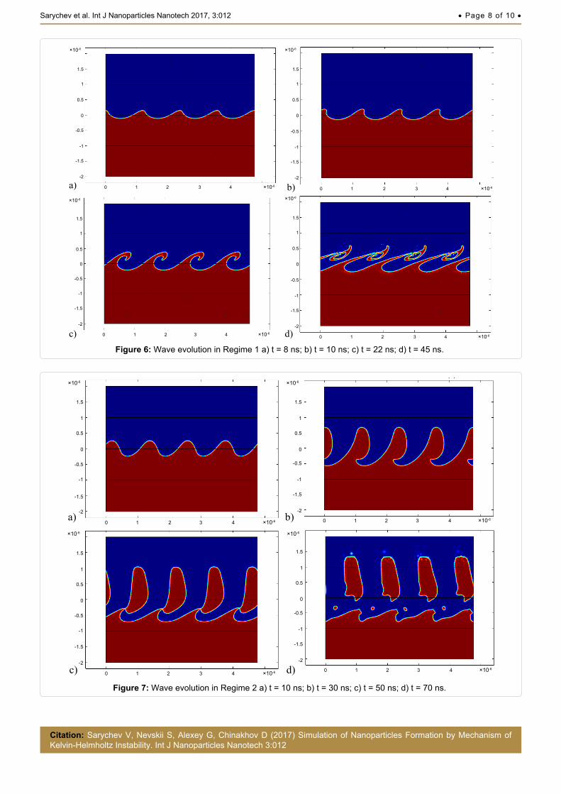
Figure 6 and Figure 7 demonstrate wave evolution at different times in different modes. It is seen that the perturbations at the interface gradually increase first in Regime 1 (Figure 6a and Figure 6b). Then, at t = 10 ns (Figure 6c) the wave front breaks down. The process of forming a vortex starts at a time of 22 ns (Figure 6d). At t > 22 ns, the vortex structure is fragmented and droplets are formed. The dimensions of these droplets range from ~90 nm to ~242 nm. In addition to the vortex breaking down into droplets, the process of merging small drop-lets into larger drops is observed in Regime 1. Thus, when we allow for the nonlinearity while investigating the Kelvin-Helmholtz instability, we can observe the two processes of forming nanosized droplets due to the de-cay of the vortex and their merging into submicrosized particles. According to linear analysis, in theses modes,

wave approximation, the dispersion equation itself co-incides with equation (16) in form, but with different coefficients:

2* * * 1*

* * * 1** * * *

2 ( ) = 0,

= , , = , 1 1 2 1 2 1 2

a ib c ica b c ca b c c

t t t t

ω ω

ω ω ω ω

+ + + +

= =− − − −

(26)

For simplicity, we assume that the time of relaxation in Layers 1 and 2 are the same. Then the dependence of the decrement α on the wavenumber is written as:

( )22 2 2* * 1 *

1*

( ) 4 11 = 1 2

t t a b ta

tδ ω δ ω δ ω

αω

− + − + − − − −

(27)

Thus, it follows from the linear analysis of the equa-tions of motion that the two-mode Kelvin-Helmholtz in-stability is observed in the case of a viscous, viscoelastic and porous medium. This means that the waves with a wavelength of λm1 and λm2 will progress. As is known, lin-ear analysis is valid only for small perturbations. In the case where the boundary is displaced from its equilibri-um position, nonlinear analysis needs to be done. The next section is devoted to nonlinear numerical analysis using the finite element method.

1 1 1 1, , ,u p µ ρ

2 2 2 2, , ,u p µ ρ

A

B C

D

x

y

Figure 5: Computation domain scheme.

Table 1: Boundary condition.

Boundary Equation Description

AB, CD = , = AB CD AB CDu u p p

Periodic boundary condition

BC u = u0 Velocity of boundaryAD P = 0 Open boundary

Table 2: Shows the values of characteristics to describe the material and the input parameters for the problem.

Characteristics Symbol ValueRegime 1 Regime 2

Lower layer thickness h 2 μm 2 μmUpper layer thickness H 2 μm 2 μmWavelength λ 1194 nm 1194 nmLongitudinal size of computational domain L 4 λ 4 λUpper layer density and Lower layer density relation A 1 10Surface tension σ 1.91 N/m 1.91 N/mLower layer viscosity μ1 10-3 Pa∙s 10-3 Pa∙sUpper layer viscosity μ2 10-5 Pa∙s 10-5 Pa∙sVelocity u0 50 m/s 50 m/s

• of 10 •



c)

a)

d)

b)

×10-6

×10-6

×10-6

1.5

1

0.5

0

-0.5

-1

-1.5

-2

×10-6

1.5

1

0.5

0

-0.5

-1

-1.5

-2

1.5

1

0.5

0

-0.5

-1

-1.5

-2

×10-6

1.5

1

0.5

0

-0.5

-1

-1.5

-2

0 1 2 3 4 ×10-60 1 2 3 4

×10-60 1 2 3 4×10-60 1 2 3 4

Figure 6: Wave evolution in Regime 1 a) t = 8 ns; b) t = 10 ns; c) t = 22 ns; d) t = 45 ns.

×10-6

×10-6 ×10-6

1.5

1

0.5

0

-0.5

-1

-1.5

-2

×10-6

1.5

1

0.5

0

-0.5

-1

-1.5

-2

×10-6×10-6

1.5

1

0.5

0

-0.5

-1

-1.5

-2

1.5

1

0.5

0

-0.5

-1

-1.5

-2

0 1 2 3 4 0 1 2 3 4

×10-6×10-6 0 1 2 3 4

0 1 2 3 4

a) b)

c) d)

Figure 7: Wave evolution in Regime 2 a) t = 10 ns; b) t = 30 ns; c) t = 50 ns; d) t = 70 ns.

• of 10 •



4. Sarychev VD, Nevskii SA, Gromov VE (2016) Model of nanostructure formation in rail steel by intensive plastic de-formation. Deformatsiya i Razrushenie Materialov 6: 25-29.

5. Sarychev VD, Nevskii SA, Sarycheva EV, Konovalov SV, Gromov VE (2016) Viscous flow analysis of the Kel-vin-Helmholtz instability for short waves. AIP Conference Proceedings 1783: 020198.

6. Batchelor GK (2000) An Introduction to Fluid Dynamics. Cambridge University Press, New york 615.

7. Joseph D, Funada T, Wang J (2008) Potential flows of vis-cous and viscoelastic fluids. Cambridge University Press, New York.

8. Al-Zubaydi ASJ, Zhilyaev AP, Shun C, Kucita WP, Reed PAS (2016) Evolution of microstructure in AZ91 alloy pro-cessed by high-pressure torsion. J Mater Sci 51: 3380-3389.

9. Zhu YT, Varyukhin V (2006) Nanostructured Materials by High-Pressure Severe Plastic Deformation. Springer, Ber-lin.

10. Tarasov SY, Rubtsov VE (2011) Shear instability in the subsurface layer of a material in friction. Physics of the Sol-id State 53: 358-362.

11. Kuznetsov VP, Smolin IYu, Dmitriev AI, Tarasov SY, Gorgots VG (2016) Toward control of subsurface strain accumulation in nanostructuring burnishing on thermostrengthened steel. Surface and Coatings Technology 285: 171-178.

12. Ning J-l, Courtois-Manara E, Kurmanaeva L, Ganeev AV, Valiev RZ, et al. (2013) Tensile properties and work hard-ening behaviors of ultrafine grained carbon steel and pure iron processed by warm high pressure torsion. Materials Science and Engineering A 581: 8-15.

13. Peregudov OA, Morozov KV, Gromov VE, Glezer AM, Ivan-ov YF (2016) Formation of internal stress fields in rails during long-term operation. Russian Metallurgy (Metally) 2016: 371-374.

14. Heisenberg W (1924) Uber Stabilitat und Turbulenz von Flussigkeitsstrornen. Annalen der Physik 74: 577-627.

15. Lin CC (1955) Theory of hydrodynamic stability. Cambridge University Press, Cambridge.

16. Fultz B, Howe J (2013) Transmission electron microscopy and diffractometry of materials. Springer, Berlin.

17. Sundeev RV, Glezer AM, Shalimova AV, Djakonov DL, Nosova GI (2012) Susceptibility of crystalline alloys to de-formational amorphization during torsion under quasihydro-static pressure. Bulletin of the Russian Academy of Scienc-es: Physics 76: 1226-1232.

18. Sundeev RV, Shalimova AV, Pechina EA, Glezer AM, Nosova GI, et al. (2015) Deformation behavior of layered amorphous-crystalline ti-ni-cu composite under different conditions of torsion in a bridgman chamber. Bulletin of the Russian Academy of Sciences: Physics 79: 1156-1161.

19. Sarychev VD, Gromov VESA, Nevskii, AI Nizovskii, SV Konovalov (2016) Nanolayer formation during hydrody-namic instability under external stimuli. Steel in Translation 46: 679-685.

20. Jiang MQ, Wilde G, Qu CB, Jiang F, Xiao HM, et al. (2014) Wavelike fracture pattern in a metallic glass: a Kelvin-Helm-holtz flow instability. Philosophical Magazine Letters 24: 669-677.

the single-mode dependences of decrement should be observed, with their maxima falling on a wavelength of 194 nm (Regime 1) In mode 2, the situation is radically different at t = 10 ns (Figure 7a), the perturbations first increase. Then, at a time of 30 ns (Figure 7b), a large drop begins to form, which at t = 50 ns (Figure 7c) breaks off. The size of these drops is ~1.53 μm. At t > 70 ns small droplets begin to form (Figure 7d) whose size is ~150 nm. According to the linear analysis (see the previous section), in this case there will be a two-mode instabil-ity. Thus, a nonlinear analysis of the Kelvin-Helmholtz instability fully confirms the results of the linear analysis.

Conclusion1. A simplified dispersion equation is obtained for

short-wave perturbations at the boundary of two vis-cous liquids. The dependence of the decrement on the wavelength for the total and the reduced dispersion equations for short waves coincide.

2. A simplified equation makes it possible to obtain an analytical dependence of the decrement on the wave-number. An analysis of this dependence showed that there exist one- and two-mode Kelvin-Helmholtz in-stability.

3. Parameters are determined under which one of the maxima of this dependence occurs in the submicro and nanorange. For viscoelastic, the same two-mode dependences are obtained.

4. The modeling of the Kelvin-Helmholtz instability in the nonlinear case for the parameters corresponding to single- and double-mode instabilities has shown a fundamental difference: For a single-mode regime, the droplet sizes lie in a narrow range of parameters, and for the two-mode regime the maximum and min-imum dimensions differ by a factor of 10.

5. The obtained results will allow not only to explain, but also to predict the conditions for the formation of nanomaterials and to select technological parameters in the formation of nanostructured states.

This research is supported by the Russain Science Foundation ( 15-12-00010).

References1. Sarychev VD, Vashchuk ES, Budovskikh EA, Gromov VE

(2010) Nanosized structure formation in metals under the action of pulsed electric-explosion-induced plasma jets. Tech Phys Lett 36: 656-659.

2. Granovskii AY, Sarychev VD, Gromov VE (2013) Model of formation of inner nanolayers in shear flows of material. Technical Physics 58: 1544-1547.

3. Funada T, Joseph DD (2001) Viscous potential flow analy-sis of Kelvin-Helmholtz instability in a channel. J Fluid Mech 445: 263-283.

http://aip.scitation.org/doi/pdf/10.1063/1.4966492




https://www.aem.umn.edu/people/faculty/joseph/archive/docs/book-00-12_master-sep20-cup-text.pdf



http://www.sciencedirect.com/science/article/pii/S0257897215304199









https://search.proquest.com/openview/6bf1a6e806f16f7a24809696f9777b23/1?pq-origsite=gscholar&cbl=326310




https://ntrs.nasa.gov/search.jsp?R=19930093939

https://ntrs.nasa.gov/search.jsp?R=19930093939

https://search.proquest.com/openview/758c2d5e96df5f6d3b263c4561ea481a/1?pq-origsite=gscholar&cbl=2044430





https://www.aem.umn.edu/people/faculty/joseph/papers/khinstabS.pdf



• of 10 •



25. Osher SJ, Fedkiw RW (2003) Level Set methods and dy-namic implicit surfaces. Springer, New York.

26. Balabel A (2015) Application of Level Set Method for Sim-ulating Kelvin-Helmholtz Instability Including Viscous and Surface Tension Effects. International Journal of Mathe-matics and Computational Science 1: 30-36.

27. Atmakidis T, Kenig EY (2010) A Study on the Kelvin-Helm-holtz Instability Using Two Different Computational Fluid Dynamics Methods. Journal of Computational Multiphase Flows 2: 33-45.

21. L Martín-Banderas, AM Gañán-Calvo, M Fernández-Aréva-lo (2010) Making Drops in Microencapsulation Processes. Letters in Drug Design & Discovery 7: 300-309.

22. Kulikovskii AG, Shikina IS (1985) On the asymptotic be-havior of localized perturbations in the presence of Kel-vin-Helmholtz instability. Fluid Dynam 20: 186-193.

23. Frenkel J (1955) Kinetic theory of liquids. Dover, New York.

24. Sussman M, Smereka P, Osher S (1994) A level set approach for computing solutions to incompressible two-phase flows. Journal of Computational Physics 114: 146-159.

http://read.pudn.com/downloads121/ebook/513851/%5b2002%5d Level Set Methods and Dynamic Implicit Surfaces.pdf

http://read.pudn.com/downloads121/ebook/513851/%5b2002%5d Level Set Methods and Dynamic Implicit Surfaces.pdf

http://journals.sagepub.com/doi/pdf/10.1260/1757-482X.2.1.33







simulation of nanoparticles formation by mechanism of...

Documents